Use of RGB Vegetation Indexes in Assessing Early Effects of Verticillium Wilt of Olive in Asymptomatic Plants in High and Low Fertility Scenarios

Abstract

Verticillium Wilt of Olive, a disease caused by the hemibiotrophic vascular fungus Verticillium dahliae Kleb. presents one of the most important constraints to olive production in the world, with an especially notable impact in Mediterranean agriculture. This study evaluates the use of RGB vegetation indexes in assessing the effects of this disease during the biotrophic phase of host-pathogen interaction, in which symptoms of wilt are not yet evident. While no differences were detected by measuring stomatal conductance and chlorophyll fluorescence, results obtained from RGB indexes showed significant differences between control and inoculated plants for indexes Saturation, a*, b*, green Area (GA), normalized green-red difference index (NGRDI) and triangular greenness index (TGI), presenting a reduction in plant growth as well as in green and yellow color components as an effect of inoculation. These results were contrasted across two scenarios of mineral fertilization in soil and soil amended with two different olive mill waste composts, presenting a clear interaction between the host-pathogen relationship and plant nutrition and suggesting the effect of V. dahliae infection during the biotrophic phase was not related to plant water status.

1. Introduction

Verticillium Wilt of Olive (VWO), a vascular disease caused by the pathogenic soil-borne fungus Verticillium dahliae Kleb, is one of the most severe threats to olive production today [1]. Taxonomic classifications place this fungus in Division Ascomycota, Class Sordariomycetes, Subclass Hypocreomycetidae, Order incertae sedis, Family Plectosphaerellaceae [2]. Other classifications place it within Deuteromycetes [3] along with other fungi without known sexual reproduction, since V. dahliae is a haploid species for which no teleomorph has been identified to date.

Verticillium dahliae (Vd) can survive short periods of time in the form of mycelium or conidia in infected perennial plants, but a specific form of melanized mycelium known as microsclerotia (MS) are the main survival structures and primary infectious propagules. MS are incorporated into soil from degrading host tissue, remaining viable for up to 14 years [4] establishing the non-parasitic phase of the biological cycle. The parasitic phase starts when favorable conditions stimulate MS germination, producing hyphae that penetrate young roots by a passive entry mechanism [5] and subsequently colonize the aerial part of the host via passive transport through the vascular system [6].

V. dahliae is a hemibiotrophic fungus that initially shows biotrophic behavior during host colonization, with minimal detrimental effects on plant physiological status. At a later stage, however, pathogen-host interaction becomes necrotrophic, a process mediated by jasmonate and salicylate phytohormone cross-talk, triggering expression of wilt symptoms when colonization is widespread with subsequent cell-death in host tissues [7]. Symptoms of wilt in olive trees include chlorotic leaves that roll inward, dead branches, defoliation and necrosis [8]. Evidence suggests the complex physiological effects of V. dahliae infection on the host are caused by vascular obstruction as well the host’s own defense mechanisms; xylem blockages may be due to mycelium itself or plant-produced aggregates such as tyloses or lignin depositions [9]. This interaction between pathogen colonization and host physiological response has been characterized to result in limits on water and nutrient transport, mimicking water deficit stress and causing stomatal closure and chlorosis, significantly reducing photosynthetic capacity through a combination of reduced chlorophyll content [10,11] and reduced CO₂ inputs, consequently downregulating photosynthesis [12,13].

Two pathogenicity groups of V. dahliae have been established, classified into defoliating (D) and non-defoliating (ND) pathotypes according to differential levels of virulence and ability to defoliate [8]. It is interesting to note that isolates recovered from olive display the same differential pathotypes and are cross-virulent in cotton (Gossypium hirsutum L.) [14] as well as pathogenic in Arabidopsis thaliana [15].

Infection in olive trees in many cases results in plant death, although trees may overcome the disease due to a combination of different factors [16]. The infection process is favored by optimum temperatures for fungal growth, ranging from 21 to 24 °C [17]; contrarily, when average temperatures linger persistently over 25 °C for a protracted period of time host colonization may stop, avoiding or reverting expression of wilt symptoms [11,18].

Management of VWO has proven to be highly difficult and commands an integrated management strategy that combines different practices, as one sole solution does not exist. Lack of success with fungicide treatments in VWO infected trees [19] highlights the importance of alternate management practices. Proposed alternatives include preventative measures such as establishing orchards with certified pathogen-free plants, selecting resistant cultivars and practices that avoid inoculum arrival [8], as well as remedial practices such as soil solarization [16]. One promising method for Verticillium wilt disease control is the use of suppressive substrates, defined as environments in which development of disease is restricted, in spite of the presence of a pathogen, a susceptible host and favorable environmental conditions [20,21]. Use of organic amendments such as compost for their suppressive properties is today a regular practice in agriculture, their efficacy widely substantiated by a number of studies. Established mechanisms of disease suppression are highly dependent on substrate micro-flora, primarily due to pathogen-antagonist interactions which may include competition for nutrients and colonization sites, hyperparasitism, antibiosis, induced systemic resistance (ISR) and systemic-acquired resistance (SAR), although physicochemical properties of amendments may also contribute by action of substances such as humic acids or enhancing plant resistance as a consequence of improved nutrition [22,23,24]. Compost elaborated from olive-mill waste has been shown to significantly reduce disease severity of Verticillium wilt in eggplant [25], as well as olive and cotton [26].

Remote sensing technologies are a novel method for assessing crop physiological status and phenotyping which has gathered increasing interest in recent years. The use of indexes derived from RGB (red-green-blue) images taken with conventional cameras is a simple, non-destructive and cost-effective method employed in assessing crop status in field conditions, including N status and water stress [27]. RGB images have proven useful in studies evaluating the effect of abiotic stresses but have yet to be fully exploited to phenotype disease resistance [28], although RGB indexes have proven to be accurate predictors of grain yield as well as in assessing damage caused by Fusarium in wheat kernels [29] or assessing grain yield losses and resistance to yellow rust in wheat [30,31]. To the author’s knowledge, although other remote sensing technologies have been used in assessing VWO, this was the first time that RGB vegetation indexes were used for this purpose.

Information captured digitally by taking pictures of plants is contained in the red, green and blue digital numbers for each pixel. When these images are processed, RGB values are converted to values in IHS (Intensity-Hue-Saturation) color space, (https://micro.magnet.fsu.edu/primer/digitalimaging/russ/colorspaces.html). Intensity represents luminance information, Hue refers to the color itself and represents the average wavelength of the color spectrum and Saturation defines the color purity from white to the corresponding primary color. These IHS values are used to obtain vegetation indexes, some of which represent proportions within an image. Indexes fitting this criteria are the green area index (GA) [32], which calculates percentage of green pixels in a given image by defining green as 60° < Hue < 180°, or the greener area index (GGA) which has a stricter definition with green as 80° < Hue < 180°, thus excluding pixels with a yellowish-green hue generally associated with senescent plant matter. The difference between these two is used to determine the crop senescence index (CSI) which estimates the percent of senescent plant matter relative to total canopy [30].

Other indexes represent different qualities of color by providing a numerical value that describes the mean obtained from the different pixels in a given image; such is the case for properties of color Intensity, Hue, Saturation and Lightness (obtained from IHS color space), as well as values obtained from color spaces CIELAB (L*a*b*) and CIELUV (L*u*v*), proposed by the CIE (Comission Internationale de l’Éclairage) and which attempt to produce an intuitive representation of human color perception. In each of these color spaces L represents lightness, with a maximum value of 100 corresponding to a perfect reflecting diffuser and a minimum value of 0 representing black. Hue is represented on a two-dimensional plane orthogonal to L* and is defined by two axes or color opponent coordinates, named a* and b* in CIELAB (Figure 1), with a* running from green (−a*) to red (+a*) and b* from blue (−b*) to yellow (+b*) on a scale from 100 to −100. Axes u* and v* in CIELUV space are analogous to a* and b* respectively, although calculated using a different formula [33]. Figure 1 details colors that correspond to the ‘green quadrant’ (−a*, +b*) of CIELAB color space.

Other indexes such as the normalized green-red difference index (NGRDI) and the triangular greenness index (TGI) may be derived from conventional images as well as from multispectral information, also contributing information relating to plant physiological status. NGRDI approximates biomass and N status, while TGI is a solid indicator of chlorophyll content and is more accurate at a canopy scale compared to NGRDI [34,35,36].

The objectives of this study were (i) to study the role of olive mill waste compost in Verticillium wilt suppressiveness, (ii) to elucidate the interaction between Verticillium infection and nutrient availability by contrasting different mixes of soil and compost in two scenarios, one with and one without mineral fertilization, iii. to test RGB vegetation indexes in detection and assessment of Verticillium wilt and contrast obtained results with classical physiological measurements.

2. Materials and Methods

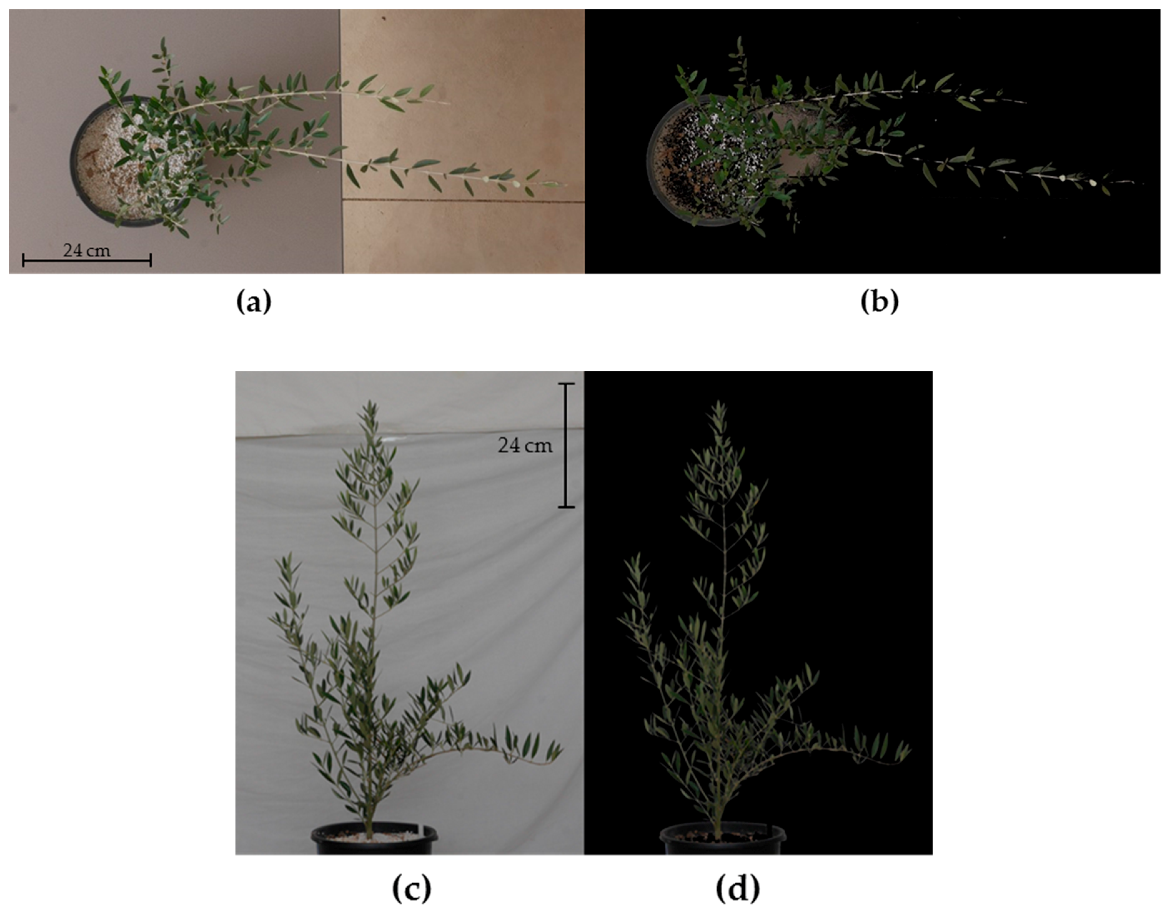
2.1. Experimental Design

In order to evaluate the effects of Verticillium Wilt of Olive in planta, a greenhouse experiment was conducted at the University of Barcelona Torribera Campus (41°27′48.4″ N 2°12′53.0″ E) employing 240 young olive tree clones (Olea europaea) of the cultivar Picual, which has been characterized as highly susceptible to Verticillium wilt [37]. Each cutting was transplanted into a 10L black plastic pot during November 2016 employing 6 distinct substrate mixes, based on a soil obtained from an olive orchard in Abrera, Catalonia, Spain in which VWO has not been detected.

Two distinct commercial olive mill waste composts (C) were used as organic amendments, henceforth referred to as compost 1 (C1) and compost 2 (C2). C1 was composed of 63% wet olive husks, 30% olive leaf waste, and 7% sheep manure, produced in an olive mill in Jaén, Spain, while C2 was composed of 50% wet olive husks, 1% olive leaf waste and 49% goat manure and straw and was produced in Málaga, Spain. Both these composts had been previously evaluated for V. dahliae microsclerotia suppressiveness by Aviles and Borrero [38]. Soil was mixed with perlite (Perlite, 2–6 mm, Premium Gramoflor, Germany) at a 2:1 ratio by volume, and this soil-perlite mix was in turn combined with composts 1 or 2 in corresponding treatments at a ratio of 4:1 (soil-perlite to compost) by volume. Resulting substrate mixes were: Soil, Soil-C1, and Soil-C2. Chemical characteristics of the soil, composts, and soil-compost mixes are detailed in

Table 1. Chemical characteristics of soil, compost and soil-compost mixes.

	pH	EC (mS cm−1)	C (%)	C/N	N (%)	P Olsen (mg/kg)	P (%)	K (%)	S (%)	Ca (%)	Mg (%)
Soil	8.58	111.8	0.86	10.75	0.08	12.4	ND	ND	ND	ND	ND
C1	9.51	3345	33.91	22.31	1.52	59.3	0.15	2.26	0.19	7.14	1.29
Soil + C1	8.81	403	2.56	15.06	0.17	21	ND	ND	ND	ND	ND
C2	8.7	3655	28.71	14.58	1.97	340	0.42	1.9	0.5	9.05	0.97
Soil + C2	8.9	650.5	2.39	11.38	0.21	63.1	ND	ND	ND	ND	ND

C1: compost 1, C2: compost 2, EC: electrical conductivity, C: organic C, P-Olsen: available P, ND: not determined.

.

Each soil-compost mix was established in two scenarios, one alone (MF-) and another supplemented with mineral fertilization (MF+). The mineral fertilizer used was ENTEC Nitrofoska 14-7-17, (EuroChem Agro, Barcelona, Spain) containing 8% ammoniacal and 6% nitric nitrogen, 7% P₂O₅, 17% K₂O, 22.5% SO₃, 2% MgO, 0.02% B, 0.01% Zn, and 0.8% 3,4-dimethylpyrazole phosphate (DMPP), applied at a dose of 142.5 Kg N ha⁻¹, 31.1 Kg P ha⁻¹ and 150.45 kg K ha⁻¹.

For each of the soils or soil-compost mixes, a control and a V. dahliae-inoculated (I) group were established, yielding a total of 6 experimental conditions in each mineral fertilization scenario. For this purpose, a V. dahliae defoliating pathotype isolate provided by Dr. Manuel Avilés (Universidad de Sevilla), obtained from 6 Petri dishes in which the fungus had grown in Czapek-Dox Agar media for 4 weeks in the dark at 28 °C, was transferred to a sterile 40 L fermenter and incubated for 5 days at an aeration rate of 6 L min⁻¹ (pO₂ was adjusted at 100 ±5%), 1000 rpm, 25 °C, and at a non-buffered pH in Czapek-Dox Broth, yielding a conidial suspension. Plants were inoculated with this suspension at 10⁶ CFU/mL soil at the beginning of the experiment and were re-inoculated once every 6 months coinciding with the start of spring and fall. Control and inoculated plants were maintained separate within the greenhouse in order to prevent cross-contamination, while plants of the different treatments were otherwise randomized. Environmental conditions were semi-controlled, since fluctuations in temperature depended on the weather, but were adjusted to some extent by controlling the opening of the greenhouse roof. Watering was carried out regularly according to plant demand and weeds were controlled manually as needed.

Of the total 240 plants, 48 were randomly selected for sampling, establishing 4 replicates for each of the 6 experimental conditions in each mineral fertilization scenario (4 replicates × 3(C) × 2(I) × 2(MF)). The current study was carried out during the springtime of the second year since the start of the experiment, with 5 samplings carried out at ±3 hours around solar noon during the last week of each month spanning from February to June 2018. Each sampling time point (T) was labeled: T1, T2, T3, T4 and T5.

2.2. Physiological Measurements

Physiological measurements were carried out separately in young and mature leaves, with young leaves selected from the third pair of new growth counting downwards from the apical meristem, and mature leaves selected based on stem width and a lower position on the plant, always maintaining a necessary minimum leaf area required for the fluorometer and porometer leaf clips.

Leaf stomatal conductance (G_s) was determined by measuring leaf abaxial epidermises using a Decagon SC-1 Leaf Porometer (Decagon Devices Inc., Pullman, Washington, USA). Chlorophyll fluorescence was measured using a MINI-PAM fluorimeter (Walz, Effeltrich, Germany) determining photosystem II quantum efficiency (ɸPSII) by exposing leaf adaxial epidermises to a 0.8s saturating flash at 6000 µmol photons m²·s¹ in vivo in daylight conditions within the greenhouse, as well as in severed leaves that were dark-adapted for 1 hour in order to determine photosystem II maximum quantum efficiency (Fv/Fm), corresponding with all chlorophyll reaction centers being open.

Soil temperature at the time of sampling leaf stomatal conductance and chlorophyll fluorescence was measured with a Decagon Pro-Check (Decagon Devices Inc., Pullman, Washington, USA).

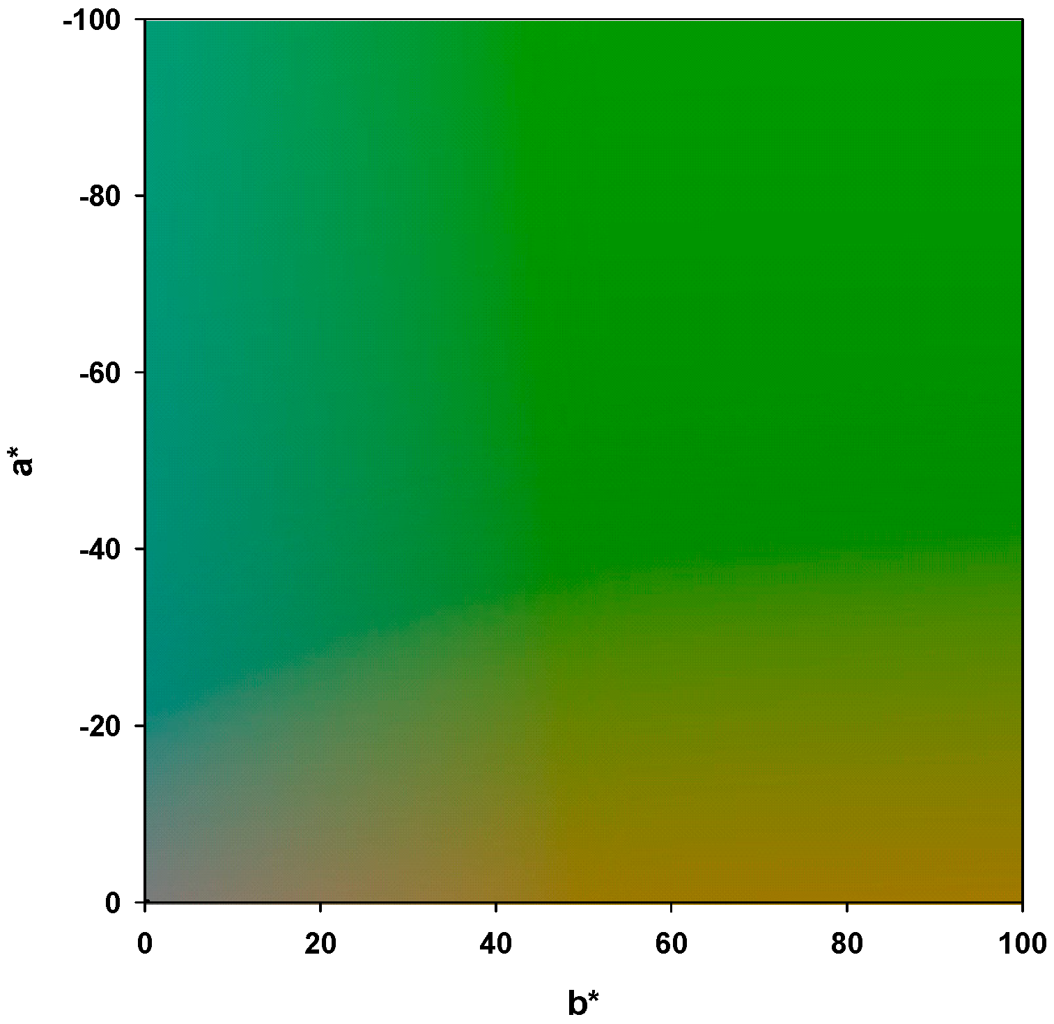
2.3. RGB Vegetation Indexes

RGB images were obtained using a Panasonic Lumix DMC-GX7 16-megapixel resolution camera (Panasonic Corporation, Osaka, Japan) with a G1:1.7/20 ASPH Φ46 0.2m/0.66ft-∞ lens, with aperture and ISO programed in automatic mode, and a Smartphone as remote shutter-release button controller through Panasonic Image App. The camera was mounted on a tripod and four images were obtained for each plant, all taken from a distance of 2.3 m from the camera to the edge of the pot: two from a zenithal plane and two from a lateral plane, rotating the plants 90° for maximum stereoscopy. The images were taken ±1 hour around solar noon under conditions of natural light inside the greenhouse, in a chamber that had translucid walls and an opaque ceiling, thus providing considerable light diffusion. Cloudy days were avoided for sampling, since passing clouds would cause undesirable immediate changes in light conditions. Images were saved in a 4592 × 3448 pixel JPG format. Gamma-correction was not applied. The mean calculated from the results obtained from each of the 4 different images taken per plant was treated as the final result.

Each image was processed using open-source software FIJI, a modified version of Image-J (https://github.com/fiji), first cropping images to desired size, and subsequently eliminating all pixels not corresponding to the plant (Figure 2), thus reducing background noise considerably. This was achieved by taking a picture in which the plant was removed from the frame immediately after every 4 plants were photographed, thus keeping changes in ambient light minimal. To all effects, for each image of each plant, another virtually identical picture was obtained without the plant. The algorithm “Difference” within FIJI “Image Calculator” (Process>Image Calculator) was then employed to subtract one image from the other creating a new image based on the premise that closely identical pixels in both images corresponded to the background and pixels that were different between images to the plant. This resulting image was converted from RGB to 8-bit grayscale (Image>Type>8-bit) in order to eliminate color, and was further treated (Image>Adjust>Threshold) via algorithm “Otsu” setting a threshold that resulted in all pixels being either black or white, effectively creating a binary mask in which white pixels represented the plant and black pixels the background. This mask was superposed (Process>Image Calculator) via the algorithm “Add” on the original image substituting ‘background’ pixels with black pixels but leaving all ‘plant’ pixels intact, effectively eliminating any information from color not corresponding to the plant in order for it to not interfere with final results.

FIJI plugin Breedpix was employed to determine different vegetation indexes based on image pixel color properties, resulting in high-resolution information calculated from pure pixels of either vegetation or background, as opposed to airborne images with aggregated pixels that combine information from vegetation and background. The CSI was determined from the formula $\mathrm{CSI}=100·\left(\mathrm{GA}-\mathrm{GGA}\right)/\mathrm{GA}.$ NGRDI was obtained from the formula: $\mathrm{NGRDI}=\left(\mathrm{Green}\mathrm{DN}-\mathrm{Red}\mathrm{DN}\right)/\left(\mathrm{Green}\mathrm{DN}+\mathrm{Red}\mathrm{DN}\right)$, with DN standing for digital number, measuring the difference between green and red band reflectances with a possible range of −1 to 1. TGI is a calculation of the area within a triangle with (λr, Rr), (λg, Rg), and (λb, Rb) as vertices, where λ is the wavelength (nm) and R is the reflectance for red (r), green (g), and blue (b) bands. Images used to determine CIELAB and CIELUV color coordinates a*, b*, u* and v*, as well as color properties Intensity, Hue, Saturation, and Lightness were further processed to eliminate black background pixels that would otherwise be factored into calculated means, therefore making it necessary to filter out this information by converting these images using Matlab (Mathworks, Natick, Massachusetts, USA) into new images lacking all black or near-black pixels by using RGB value ≤ 20, 20, 20 as a threshold. For the purpose simplifying analysis of results, values obtained for index a* (which were in all cases negative since green hues are represented by a* values between 0 and −100) were converted to their absolute value, and are therefore expressed as positive.

2.4. Leaf Pigment Extractions

In order to better understand changes in color detected by RGB vegetation indexes, starting at time point two (T2), one young and one mature leaf were severed from each plant and stored at −20 °C. Chlorophyll a, chlorophyll b, and total carotenoids were extracted and quantified by the method of Hiscox and Israelstam [39] with slight modifications. 50 mg of leaf fresh weight were obtained from each leaf and cut into thin strips (~1 mm wide) and placed in vials containing 3.5 mL dimethyl-sulphoxide (DMSO) and incubated at 65 °C for 4 h. Liquid extracts were transferred to a graduated tube and made up to 5 mL. OD values at 665.1, 649.1 and 480 nm were read using a spectrophotometer against a DMSO blank. Equations from Sumanta et al. [40] were used to determine concentrations (μg/mL) of chlorophyll a (Chl a), chlorophyll b (Chl b) and total carotenoids (Car): $\mathrm{Chl}\mathrm{a}=12.47·\mathrm{Abs}665.1-3.62·\mathrm{Abs}649.1$, $\mathrm{Chl}\mathrm{b}=25.06·\mathrm{Abs}649.1-6.5·\mathrm{Abs}665.1$, $\mathrm{Car}=\left(1000·\mathrm{Abs}480-1.29·\mathrm{Chl}\mathrm{a}-53.78·\mathrm{Chl}\mathrm{b}\right)/220$. Results were later adjusted to μg pigment/mg FW and the mean value obtained from the young and mature leaf sampled from each plant was used as the final result per replicate.

2.5. Data Analysis

Data was processed using Centurion Statgraphics XVII (Statpoint Technologies Inc., Warrenton, Virginia, USA) to test for statistically significant differences between treatments using a Repeated Measures Analysis of Variance (rANOVA) with significance at p ≤ 0.05. Fisher’s LSD test at p ≤0.05 was used for multiple comparisons and to check for factor significance at each time point. The Kolmogorov-Smirnov test was used to check for normality of residues, and non-normal distributions were transformed before analysis. Mauchly’s sphericity test was used and in cases in which this assumption was violated the Huynh-Feldt correction was applied when epilson > 0.75 and the Greenhouse–Geisser correction when epsilon < 0.75. Data is provided in the Supplementary Materials.

3. Results

During the course of the experiment inoculated plants remained asymptomatic, presenting no evidence of wilt. We were however, able to positively re-isolate and identify Verticillium dahliae from branch segments obtained from inoculated plants and grown out in Petri dishes in Czapek-Dox agar medium [41]. Soil temperatures recorded at the time of sampling physiological parameters (Figure 3) had a mean value of 22.8 °C at T1, 25 °C at T2, 27.3 °C at T3, 29.1 °C at T4 and 31.3 °C at T5.

3.1. Physiological Measurements

Results obtained from physiological measurements carried out to determine ɸPSII, Fv/Fm and G_s did not present significant differences between control and inoculated treatments (

Table 2. p-values obtained from rANOVA for the experimental factors without mineral fertilization (MF-) and with mineral fertilization (MF+).

	MF-				MF+
Physiological Parameters	Overall	I	C	T	Overall	I	C	T
ΦPSII Y	0.0000	NS	NS	0.0000	0.0074	NS	NS	0.0000
Fv/Fm Y	0.0000	NS	NS	0.0000	0.0001	NS	NS	NS
Gs Y	0.0000	NS	NS	0.0000	0.0014	NS	NS	0.0000
ΦPSII M	0.0027	NS	0.0294	0.0000	0.0018	NS	0.0000	0.0000
Fv/Fm M	0.0000	NS	0.0245	0.0000	0.0005	NS	0.0001	0.0015
Gs M	0.0001	NS	NS	0.0000	0.0095	NS	NS	0.0000
RGB Indexes
Intensity	0.0000	NS	0.0126	0.0000	0.0000	NS	0.0005	0.0000
Hue	0.0000	NS	0.0019	0.0000	0.0000	NS	0.0480	0.0000
Saturation	0.0000	0.0260	0.0026	0.0000	0.0000	NS	0.0007	0.0000
Lightness	0.0000	NS	NS	0.0000	0.0000	NS	0.0001	0.0000
a*	0.0000	0.0129	0.0000	0.0000	0.0000	NS	0.0014	0.0000
b*	0.0000	0.0399	0.0256	0.0000	0.0000	NS	NS	0.0000
u*	0.0000	NS	0.0000	0.0000	0.0000	NS	0.0007	0.0000
v*	0.0000	NS	NS	0.0000	0.0000	NS	NS	0.0000
GA	0.0000	0.0213	0.0000	0.0000	0.0000	NS	0.0004	0.0000
GGA	0.0000	NS	0.0000	0.0000	0.0000	NS	0.0000	0.0000
CSI	0.0000	NS	NS	0.0000	0.0000	NS	0.0014	0.0000
NGRDI	0.0000	0.0452	0.0000	0.0000	0.0000	NS	0.0006	0.0000
TGI	0.0000	0.0301	0.0000	0.0000	0.0000	NS	0.0004	0.0000
Pigment Extractions
Chl a	0.0000	0.0375	0.0012	0.0000	0.0395	NS	NS	0.0101
Chl b	0.0000	0.0049	0.0000	0.0000	0.0339	NS	NS	0.0036
Chl a+b	0.0000	0.0194	0.0000	0.0000	0.0050	NS	NS	0.0009
Car	0.0005	0.0041	0.0000	NS	0.0050	NS	0.0380	0.0000
Car/Chl ratio	0.0000	NS	NS	0.0000	0.0017	NS	NS	0.0000

C: compost, I: inoculation, T: time, ΦPSII: photosystem II quantum efficiency, Fv/Fm: photosystem II maximum quantum efficiency Gs: stomatal conductance, GA: green area index, GGA: greener area index, CSI: crop senescence index, NGRDI: normalized red-green difference index, TGI: triangular greenness index, Chl: chlorophyll, Car: carotenoids, Y: young leaves, M: mature Leaves, NS: not significant.

). Chlorophyll fluorescence measurements (ɸPSII, Fv/Fm) did however prove sensitive to compost amendments in mature leaves in both MF scenarios, showing significantly lower values for Soil-C1 plants when compared with Soil and Soil-C2 plants (

Table 3. Means obtained from soil and soil-compost mixes without mineral fertilization (MF-) and with mineral fertilization (MF+).

	MF-			MF+
Physiological Parameters	Soil	Soil-C1	Soil-C2	Soil	Soil-C1	Soil-C2
PSII Y	0.633 a	0.650 a	0.621 a	0.704 a	0.693 a	0.690 a
Fv/Fm Y	0.780 a	0.778 a	0.787 a	0.809 a	0.786 a	0.803 a
PSII M	0.650 a	0.548 b	0.650 a	0.726 a	0.525 b	0.709 a
Fv/Fm M	0.760 ab	0.658 b	0.779 a	0.792 a	0.635 b	0.784 a
RGB Indexes
Saturation	0.119b	0.115 b	0.132 a	0.120 b	0.116 b	0.129 a
Hue	73.854 b	76.472 a	77.043 a	77.791 b	77.986 b	79.475 a
a*	5.898 b	6.087 b	6.644 a	6.390 b	6.210 b	6.695 a
b*	12.731 b	12.541 a	13.402 a	12.7432 a	12.528 a	12.884 a
u*	1.564 c	1.881 b	2.226 a	2.174 b	2.040 b	2.471 a
v*	14.129 a	13.948 a	14.727 a	14.118 a	13.912 a	14.011 a
GA	1.200 b	1.635 a	1.707 a	2.863 b	3.137 b	3.573 a
GGA	0.675 b	1.333 a	1.494 a	1.531 b	1.545 b	1.945 a
CSI	55.314 a	51.563 a	50.106 a	47.779 b	51.839 a	46.219 b
NGRDI	-0.012 c	0.022 b	0.044 a	0.041 b	0.031 b	0.063 a
TGI	20.370 c	31.255 b	39.117a	35.401 b	34.676 b	42.650 a
Pigment Extractions
Chl a	0.594 b	0.731 a	0.771 a	0.888 a	0.915 a	0.919 a
Chl b	0.309 b	0.372 a	0.386 a	0.414 a	0.436 a	0.430 a
Chl a + b	0.902 b	1.103 a	1.157 a	1.302 a	1.351 a	1.349 a
Car	0.227 b	0.259 a	0.266 a	0.267 b	0.293 a	0.278 ab
Car/Chl	0.264 a	0.242 a	0.234 a	0.207 a	0.219 a	0.208 a

Different letters denote statistically significant differences (Fisher’s LSD multiple range test, p-value ≤ 0.05), C1: compost 1, C2: compost 2, ΦPSII: photosystem II quantum efficiency, Fv/Fm: photosystem II maximum quantum efficiency, GA: green area index, GGA: greener area index, CSI: crop senescence index, NGRDI: normalized red-green difference index, TGI: triangular greenness index, Chl: chlorophyll, Car: carotenoids, Y: young leaves, M: mature Leaves.

). Values obtained for Gs were only significantly affected by the sampling time point (Table 2).

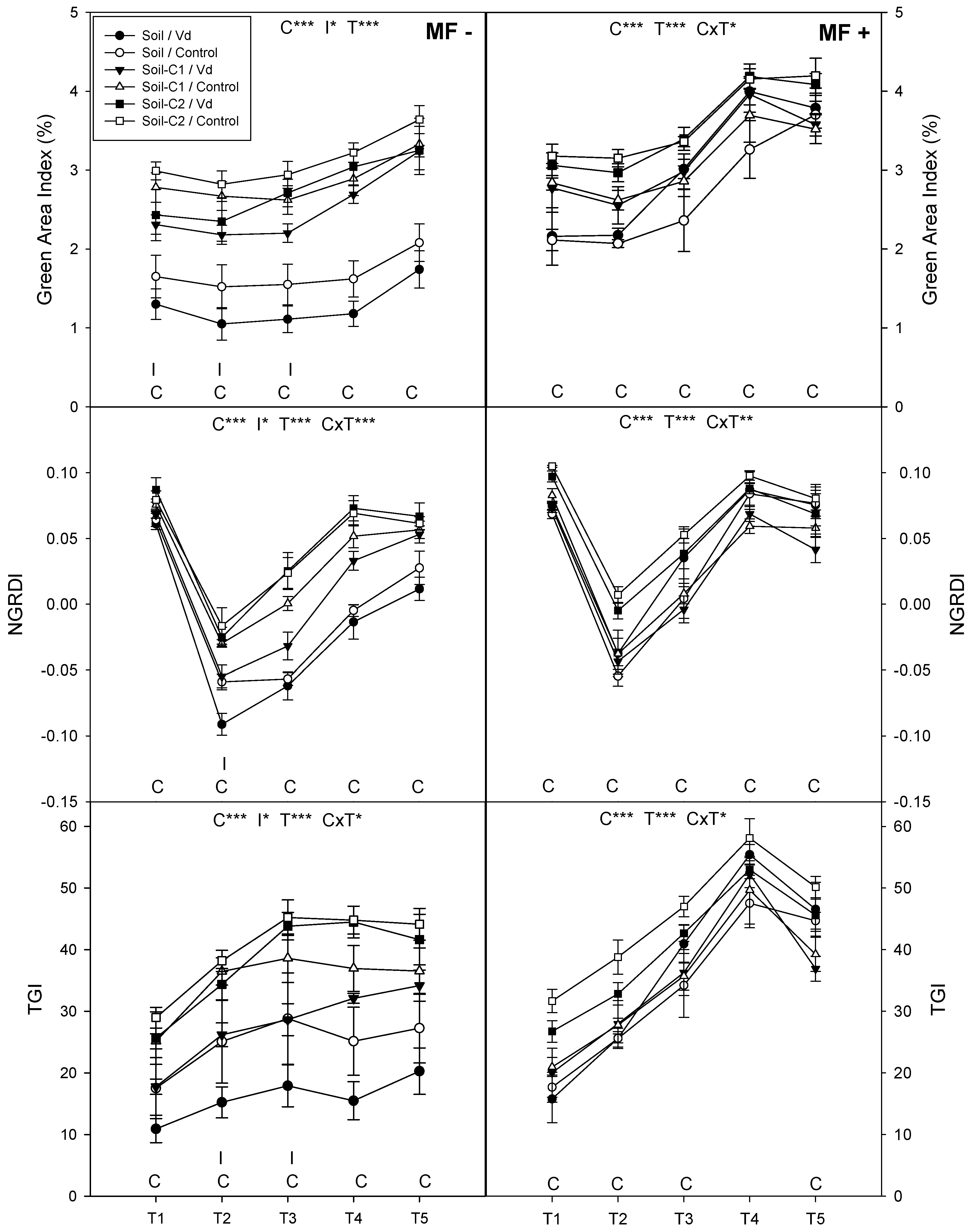
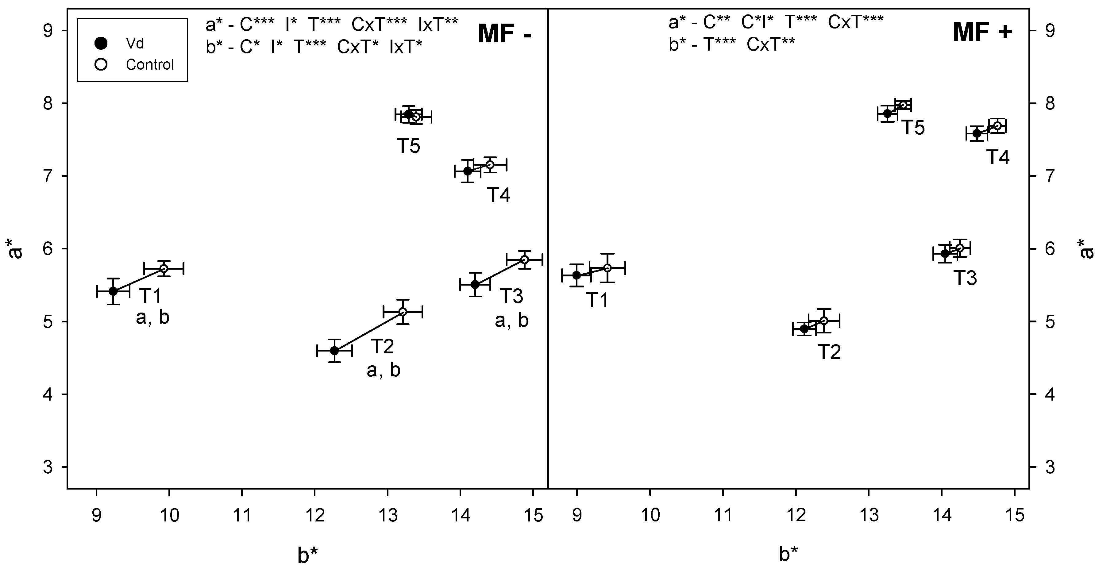
3.2. RGB Vegetation Indexes

RGB vegetation indexes Saturation, a*, b*, GA, NGRDI and TGI showed significant differences between control and inoculated plants in the MF- scenario (Table 2), while inoculation was not significant in MF+. All RGB indexes except lightness, v* and CSI were sensitive to compost amendments in the MF- scenario, and all except b* and v* in MF+. As for the effect of compost (Table 3), results obtained from RGB indexes measuring greenness (a*, u*, GA, GGA, NGRDI, TGI) in all cases showed higher values in correspondence with the addition of compost in MF-.

Index a* showed significantly higher values in Soil-C2 compared with Soil-C1 and Soil, GA and GGA showed higher values in Soil-C2 and Soil C1 compared with Soil, and values for u*, NGRDI and TGI increased significantly from those obtained for Soil when C1 was added, and once again when comparing Soil-C2 to Soil-C1. Indexes measuring yellow hues proved less sensitive, since only b* showed a significant increase in obtained values with the addition of compost. A significant increase in Hue was observed in compost amended treatments compared with Soil, while in the case of Saturation an increase was significant in Soil-C2 compared with Soil-C1 and Soil. Results obtained in the MF+ scenario showed a similar trend, with compost amended plants showing higher values for most parameters when compared with non-amended plants, although differences between the three soil-compost mixes were in certain cases reduced. Overall values obtained in MF+ increased in comparison with MF- for Hue and indexes measuring greenness, and remained similar or showed a slight reduction for Saturation and indexes measuring yellow hues.

Upon representing results obtained for RGB indexes GA, NGRDI and TGI, such that each combination of soil mix and inoculation is shown at each time point (Figure 4), it is evident in MF- that results obtained from Soil treatments were the overall lowest, while the addition of C1 showed an increase in obtained values, and the addition of C2 a further increase. Values obtained from inoculated plants were lower than their respective controls, although differences due to inoculation were reduced in both compost treatments for GA and in Soil-C2 for NGRDI and TGI, a trend that is accentuated at T4 and T5, resulting in the inoculation factor overall only showing statistical significance for GA between T1 and T3, at T2 for NGRDI and T2 and T3 for TGI. In comparison, values obtained from MF+ show that values from Soil treatments were higher than in MF-, with mean values closer to those obtained from compost treatments. Values in the MF+ scenario did not show significant differences due to inoculation, and differences between soil mixes were reduced, although in general Soil-C2 presented the highest values.

Values obtained from CIELAB color space represented as a function of a* and b* color-opponent coordinates graphically represent mean pixel color on a two dimensional-plane (Figure 5). Differences between the means obtained for control or inoculated treatments depict the inoculation effect vector at the different sampled time points. In both MF- and MF+, inoculated treatments showed a reduction of a* and a reduction of b* when compared with controls in all cases except at T5 in MF-, where a negligible increment in a* could be observed. Significant differences in vector magnitude between controls and inoculated plants for both a* and b* color opponent coordinates were found in MF- at time points T1, T2 and T3, coinciding with the early season samplings, while no significant differences were observed in vector direction in either MF- or MF+.

3.3. Leaf Pigment Extractions

Values obtained from pigment extractions detected significant differences due to inoculation in the MF- scenario (except for the case of the Car/Chl ratio), while values obtained from MF+ were not sensitive to inoculation (Table 2). Compost treatments (Table 3) also showed significantly higher pigment concentrations compared to soil in MF-, while in MF+ the only result that proved sensitive to compost amendments was carotenoid content, which was significantly lower in Soil when compared with Soil-C1, with Soil-C2 showing intermediate values.

Results obtained for chlorophyll a, chlorophyll b, and total carotenoid concentrations from the different treatments across sampling time points T2–T5 (Figure 6) showed less consistent trends when compared with RGB indexes. Significant differences due to inoculation were observed in MF-, and although overall, values were higher in inoculated treatments, T3 shows a reversal of this tendency for Soil-C1 plants in all three measurements as well as for the Soil treatment for carotenoid concentrations, while T4 shows lower values of Chl a for inoculated Soil-C1 plants. Differences due to compost were also significant for all three pigment measurements in MF-, presenting lower values in Soil treatments compared with Soil-C1, and in turn with Soil-C2, changes in this trend at certain time points resulted in the compost and time interaction being significant for all three pigment measurements. Similarly to what was observed for RGB indexes, values obtained from Soil treatments in the MF+ scenario were overall higher when compared to MF-, and differences due to inoculation or compost treatments were reduced, such that the only significant factor in MF+ was time.

Correlations between values obtained from pigment extractions and RGB indexes (

Table 4. Correlation coefficients (r) obtained from RGB vegetation indexes and chlorophyll and carotenoid extractions.

MF	Measure	hue	sat	a*	b*	a*/b*	GA	GGA	CSI	NGRDI	TGI
MF-	Chl a	0.5394 ***	−0.2239 *	0.3855 ***	−0.2792 ***	0.5304 ***	0.3762 ***	0.5236 ***	−0.5235 ***	0.4654 ***	NS
	Chl b	0.6435 ***	NS	0.5349 ***	NS	0.6324 ***	0.4862 ***	0.6437 ***	−0.6273 ***	0.5634 ***	0.2469 *
	Chl a + b	0.5937 ***	−0.2037 *	0.4477 ***	−0.2391 *	0.5837 ***	0.4258 ***	0.5823 ***	−0.5771 ***	0.5148 ***	NS
	Car	NS	NS	NS	NS	NS	0.3625 ***	0.2756 ***	NS	0.2758 **	0.2850 **
	Car/Chl	−0.6044 ***	0.2381 *	−0.4592 ***	0.2832 **	−0.6027 ***	−0.2928 **	−0.5375 ***	0.6247 ***	−0.4567 ***	NS
MF+	Chl a	NS	NS	NS	−0.3043 **	0.2624 **	NS	NS	NS	NS	NS
	Chl b	0.4188 ***	NS	0.2912 **	NS	NS	0.2568 *	0.3153 **	−0.3497 ***	0.2410 *	NS
	Chl a + b	0.2457 *	NS	NS	−0.261 *	0.2147 *	NS	NS	NS	NS	NS
	Car	−0.2672 **	NS	−0.3617 ***	−0.2624 **	0.2219 *	−0.2434 *	−0.3596 ***	0.3570 ***	−0.3240 **	−0.3096 **
	Car/Chl	−0.5936 ***	NS	−0.4778 ***	NS	NS	−0.3984 ***	−0.5437 ***	0.5826 ***	−0.4294 ***	−0.2582 *

Chl: chlorophyll concentration, Car: total carotenoids concentration, r: Pearson’s product-moment correlation coefficient, *: p-value ≤ 0.05, **: p-value ≤ 0.01, ***: p-value ≤ 0.001, NS: not significant, MF-: without mineral fertilization, MF+: with mineral fertilization, GA: green area index, GGA, greener area index, CSI: crop senescence index, NGRDI: normalized red-green difference index, TGI: triangular greenness index.

), expressed as Pearson’s r-value, generally range between 0.2 and 0.6 (positive or negative) with overall stronger correlations found in the MF- scenario. Chl b and the Car/Chl ratio showed the strongest correlations with RGB indexes in MF-, while in MF+ the strongest correlations were with the Car/Chl ratio and carotenoid concentrations, followed by Chl b. Positive correlations were found between chlorophyll contents and RGB indexes measuring green, as well as the Car/Chl ratio and indexes measuring yellow, while negative correlations were found between chlorophyll contents and indexes measuring yellow or the Car/Chl ratio and indexes measuring green. In the case of carotenoid contents, correlations did not follow a consistent trend.

4. Discussion

V. dahliae infection has been characterized as consistent with water deficit stress as a consequence of xylem blockages caused by the fungus as well as host defense mechanisms [9,42,43]. Results obtained for stomatal conductance and chlorophyll fluorescence in this study (Table 2) did not show differences due to inoculation, and since both these parameters may be used as indicators of water status these results suggest effects that mimic water stress were not present, notwithstanding other physiological changes detected. This lack of symptoms and an apparently slow disease progress may be explained by the putative disease suppressiveness of the soil-compost mixes employed as well as environmental conditions, given that the olive cultivar Picual is highly susceptible to Verticillium wilt [37,44] and the fact the defoliating pathotype V. dahliae employed in this study has been characterized as more virulent than the non-defoliating pathotype [8].

Of the environmental conditions affecting our plant pathosystem, temperature may have played a defining role in slowing disease development, since values recorded at sampling times T3-T5 (Figure 3) were in a range that has been characterized as detrimental to fungal growth for Verticillium [18], purportedly allowing the biotrophic host-pathogen interaction to stagnate and impede its progress to the necrotrophic phase. In fact, in agricultural settings, expression of wilt symptoms has been characterized to occur in the springtime and fall coinciding with favorable ambient temperatures, while yearly variations in temperature also cause a much slower disease progress when compared to that observed in growth chamber experiments with a constantly favorable temperature for fungal growth [11]. The results obtained from RGB indexes (Figure 4 and Figure 5) generally show significant differences due to inoculation from T1 to T3, when temperatures were under 27 °C. A lack of differences detected for stomatal conductance suggests xylem blockages causing symptoms similar to water deficit stress may not occur in the biotrophic phase and possibly be exclusive of necrotrophic host-Vd interactions.

As detailed in Figure 1, a reduction in both green and yellow color components in CIELAB space tend toward gray, in effect reducing color saturation, and therefore coinciding with significantly lower values obtained for Saturation in inoculated plants. In this light, differences in the inoculation effect vector observed in Figure 5 can be described as (i) changes in vector magnitude, therefore a CIELAB equivalent to the Saturation result obtained from IHS space, or (ii) changes in vector direction, defined by the a*/b* ratio and equivalent in CIELAB space to the Hue result calculated from IHS, further supported by the highly similar correlations with pigment concentrations obtained for Hue and the a*/b* ratio (Table 4).

The fact that the lower values obtained from indexes GA, NGRDI and TGI in inoculated plants were more pronounced in absence of compost amendments in the MF- scenario, coupled with the fact that values obtained for Soil treatments from indexes GA, NGRDI and TGI (Figure 4) were higher in the MF+ scenario compared with MF-, as well as higher in general in the presence of compost amendments (Table 3) suggests host-pathogen interactions in inoculated plants had an effect that acted in an opposite direction to plant nutrition. This hypothesis is further substantiated by generally higher values found in Soil-C2 compared with Soil-C1, considering Soil-C2 was more fertile (Table 1), results obtained for GA (Figure 4) which highly correlate with plant biomass [45] inferring increased plant growth as a consequence of mineral fertilization and compost amendments along with decreased plant growth due to inoculation, as well as a reduction in the inoculation effect vector magnitude when comparing MF+ to MF- (Figure 5), with no important changes in vector direction observed between mineral fertilization scenarios or across sampling time points. These findings, showing a clear interaction between host infection and nutrition are in accordance with results obtained in an assay carried out during the previous year employing the same experimental design [41], which showed reductions in leaf growth as well as reduced leaf N, K and S inputs in inoculated plants. Reduced differences observed between control and inoculated plants in results obtained from RGB indexes can thus be attributed to improved nutrition conferred by both mineral and organic fertility, although suppressiveness as a consequence of microbial activity from compost amendments cannot be ruled out and calls for further study.

The relationship between the observed changes in plant color inferred from RGB indexes and the results obtained from pigment extractions was, however, not clear-cut. Chlorophyll and carotenoid concentrations (Table 3) were higher in the MF+ scenario compared with MF-, and concentrations in the MF- scenario were higher in compost amended treatments when compared with Soil, coinciding with increases in green due to both compost and MF, measured by a*, u*, GA, GGA, NGRDI, and TGI, and decreases in yellow color, measured by b* for compost and MF and v* and CSI for MF.

In the case of inoculation however, results showed lower values of GA, NGRDI and TGI in inoculated plants in MF- (Figure 4), as well as a reduction in both green and yellow color components corresponding to a* and b* (Figure 5), while chlorophyll and carotenoid concentrations were slightly higher in inoculated plants (Figure 6), suggesting symptoms of chlorosis characterized in the literature as a consequence of Verticillium wilt [46,47] may correspond to the necrotrophic phase. These findings seem to indicate that the relationship between pigments and plant color inferred from RGB indexes is complex and may depend on other factors not contemplated by our statistical model, such as leaf thickness or leaf angle in relation to the plant, since abaxial and adaxial leaf surfaces present clear differences of color in olive plants.

Results obtained for pigment concentrations and RGB indexes (Table 4) showed significant correlations, and excepting those obtained for carotenoids, in all cases Pearson’s r-values pairing indexes measuring green with chlorophyll contents, or yellow with the Car/Chl ratio were positive, while an opposite pairing resulted in negative values. It is likely the effect of improved nutrition as a consequence of mineral fertilization and compost was the main factor contributing to positively to these correlations, with the opposite effect due to inoculation presumably subtracting from them. In fact, the lack of a consistent trend observed for correlations between RGB indexes and carotenoid contents is not remarkable, since estimation of carotenoid contents from spectral reflectance has proven difficult due to an overlap in chlorophyll and carotenoid absorption peaks, with estimation of Car/Chl ratio proving more successful [48]. The fact that the Car/Chl ratio showed high correlations overall in both MF- and MF+ scenarios can be thus interpreted as not coincidental, since perceived color is logically a result of the overlap of pigments of different colors. Since this ratio did not show, by itself, significant differences between control and inoculated plants, the changes in color measured by RGB indexes may not depend solely on leaf pigmentation, since the effect of an increase in both pigments’ concentration due to inoculation that does not substantially modify their ratio may be offset by other factors, not entirely explaining nor contradicting results measured from RGB image analysis method.

5. Conclusions

This study presents evidence suggesting the effects of V. dahliae infection during the biotrophic phase have little or no relation to water deficit stress and a strong interaction with plant nutrition, showing an opposite effect to both organic and mineral fertilization, since in cases in which values obtained for the studied parameters in inoculated plants were lower than controls, organic or mineral fertilization resulted in higher values.

Compost amendments and mineral fertilization reduced the effect of the pathogen as measured from image analysis, suggesting improved plant nutrition may contribute positively towards plant disease tolerance in Verticillium Wilt of Olive.

RGB vegetation indexes, widely used in plant phenotyping and in assessing abiotic stress, showed considerable resolution in detecting changes in plant color that could be attributed to the inoculation factor, especially notable in a context of a lack of wilting symptoms. Although remote sensing methods have already proven effective in assessing VWO symptomatic plants showing considerable wilt, this study presents data showing promise in early detection of VWO as well as other biotic stress detection and assessment, warranting further study in order to develop reliable methods of detection that may be used with images obtained from aerial platforms as a cost-effective method for scanning large areas in field scenarios. The main challenge to be faced in future applications is differentiating between the effects of biotic and abiotic stress, due to complex interactions present between crop physiological status and pathogen infection.

References

1. Keykhasaber, M.; Pham, K.T.K.; Thomma, B.P.H.J.; Hiemstra, J.A. Reliable detection of unevenly distributed Verticillium dahliae in diseased olive trees. Plant Pathol. 2017, 66, 641–650. [Google Scholar] [CrossRef]
2. Inderbitzin, P.; Bostock, R.M.; Davis, R.M.; Usami, T.; Platt, H.W.; Subbarao, K.V. Phylogenetics and taxonomy of the fungal vascular wilt pathogen Verticillium, with the descriptions of five new species. PLoS ONE 2011, 6. [Google Scholar] [CrossRef] [PubMed]
3. Messner, R.; Schweigkofler, W.; Ibl, M.; Berg, G.; Prillinger, H. Molecular characterization of the plant pathogen Verticillium dahliae Kleb. Using RAPD-PCR and sequencing of the 18SrRNA-Gene. J. Phytopathol. 1996, 144, 347–354. [Google Scholar] [CrossRef]
4. Wilhelm, S. Longevity of the Verticillium wilt fungus in the laboratory and field. Phytopathology 1955, 45, 180–181. [Google Scholar]
5. Prieto, P.; Navarro-Raya, C.; Valverde-Corredor, A.; Amyotte, S.G.; Dobinson, K.F.; Mercado-Blanco, J. Colonization process of olive tissues by Verticillium dahliae and its in planta interaction with the biocontrol root endophyte Pseudomonas fluorescens PICF7. Microb. Biotechnol. 2009, 2, 499–511. [Google Scholar] [CrossRef] [PubMed]
6. Pegg, G.; Brady, B. Verticillium Wilts; CAB International: Wallingford, UK, 2002. [Google Scholar]
7. Scholz, S.S.; Schmidt-Heck, W.; Guthke, R.; Furch, A.C.U.; Reichelt, M.; Gershenzon, J.; Oelmüller, R. Verticillium dahliae-Arabidopsis interaction causes changes in gene expression profiles and jasmonate levels on different time scales. Front. Microbiol. 2018, 9, 1–19. [Google Scholar] [CrossRef] [PubMed]
8. López-Escudero, F.J.; Mercado-Blanco, J. Verticillium wilt of olive: A case study to implement an integrated strategy to control a soil-borne pathogen. Plant Soil 2011, 344, 1–50. [Google Scholar] [CrossRef]
9. Fradin, E.F.; Thomma, B.P.H.J. Physiology and molecular aspects of Verticillium wilt diseases caused by V. dahliae and V. albo-atrum. Mol. Plant Pathol. 2006, 7, 71–86. [Google Scholar] [CrossRef] [PubMed]
10. Roca, L.F.; Moral, J.; Trapero, C.; Blanco-López, M.Á.; López-Escudero, F.J. Effect of inoculum density on Verticillium wilt incidence in commercial olive orchards. J. Phytopathol. 2016, 164, 61–64. [Google Scholar] [CrossRef]
11. Calderón, R.; Lucena, C.; Trapero-Casas, J.L.; Zarco-Tejada, P.J.; Navas-Cortés, J.A. Soil temperature determines the reaction of olive cultivars to Verticillium dahliae pathotypes. PLoS ONE 2014, 9. [Google Scholar] [CrossRef] [PubMed]
12. Bowden, R.L.; Rouse, D.I.; Sharkey, T.D. Mechanism of photosynthesis decrease by Verticillium dahliae in potato. Plant Physiol. 1990, 94, 1048–1055. [Google Scholar] [CrossRef] [PubMed]
13. Sadras, V.O.; Quiroz, F.; Echarte, L.; Escande, A.; Pereyra, V.R. Effect of Verticillium dahliae on photosynthesis, leaf expansion and senescence of field-grown sunflower. Ann. Bot. 2000, 86, 1007–1015. [Google Scholar] [CrossRef]
14. Mercado-Blanco, J.; Rodriguez-Jurado, D.; Pérez-Artés, E.; Jiménez-Díaz, R.M. Detection of the nondefoliating pathotype of Verticillium dahliae in infected olive plants by nested PCR. Plant Pathol. 2001, 50, 609–619. [Google Scholar] [CrossRef]
15. Maldonado-González, M.M.; Bakker, P.A.H.M.; Prieto, P.; Mercado-Blanco, J. Arabidopsis thaliana as a tool to identify traits involved in Verticillium dahliae biocontrol by the olive root endophyte Pseudomonas fluorescens PICF7. Front. Microbiol. 2015, 6, 1–12. [Google Scholar] [CrossRef] [PubMed]
16. Tjamos, E.C. Recovery of olive trees with Verticillium wilt after individual application of soil solarization in established olive orchards. Plant Dis. 1991, 75, 557. [Google Scholar] [CrossRef]
17. Bejarano-AIcazar, J. Etiology, Importance, and distribution of Verticillium wilt of cotton in Southern Spain. Plant Dis. 1996, 80, 1233. [Google Scholar] [CrossRef]
18. Isaac, I. A Comparative study of pathogenic isolates of Verticillium. Trans. Br. Mycol. Soc. 1949, 32, 137-IN5. [Google Scholar] [CrossRef]
19. Jiménez-Díaz, R.M.; Cirulli, M.; Bubici, G.; del Mar Jiménez-Gasco, M.; Antoniou, P.P.; Tjamos, E.C. Verticillium wilt, a major threat to olive production: Current status and future prospects for its management. Plant Dis. 2012, 96, 304–329. [Google Scholar] [CrossRef] [PubMed]
20. Baker, K.F.; Cook, R.J. Biological control of plant pathogens. Am. Phytopathol. Soc. St. Paul MN 1974. [Google Scholar] [CrossRef]
21. Avilés, M.; Borrero, C.; Trillas, M.I. Review on compost as an inducer of disease suppression in plants grown in soilless culture. Dyn. Soil Dyn. Plant 2011, 5, 1–11. [Google Scholar]
22. Segarra, G.; Santpere, E.; Elena, G.; Trillas, M.I. Enhanced Botrytis cinerea resistance of Arabidopsis plants grown in compost may be explained by increased expression of defense related genes, as revealed by microarray analysis. PLoS ONE 2013, 8. [Google Scholar] [CrossRef] [PubMed]
23. Segarra, G.; Elena, G.; Trillas, I. Systemic Resistance against Botrytis cinerea in Arabidopsis triggered by an olive marc compost substrate requires functional SA signalling. Physiol. Mol. Plant Pathol. 2013, 82, 46–50. [Google Scholar] [CrossRef]
24. Raviv, M. Compost as a tool to suppress plant diseases: Established and putative mechanisms. Acta Hortic. 2016, 1146, 11–24. [Google Scholar] [CrossRef]
25. Papasotiriou, F.G.; Varypatakis, K.G.; Christofi, N.; Tjamos, S.E.; Paplomatas, E.J. Olive Mill Wastes: A source of resistance for plants against Verticillium dahliae and a reservoir of biocontrol agents. Biol. Control 2013, 67, 51–60. [Google Scholar] [CrossRef]
26. Castaño, R.; Avilés, M. Factors that affect the capacity of growing media to suppress Verticillium wilt. Acta Hortic. 2013, 1013, 465–471. [Google Scholar] [CrossRef]
27. Vergara-Díaz, O.; Zaman-Allah, M.A.; Masuka, B.; Hornero, A.; Zarco-Tejada, P.; Prasanna, B.M.; Cairns, J.E.; Araus, J.L. A novel remote sensing approach for prediction of maize yield under different conditions of nitrogen fertilization. Front. Plant Sci. 2016, 7, 1–13. [Google Scholar] [CrossRef] [PubMed]
28. Kefauver, S.C.; El-Haddad, G.; Vergara-Diaz, O.; Araus, J.L. RGB Picture vegetation indexes for high-throughput phenotyping platforms (HTPPs). Remote. Sens. Agr. Ecosyst. Hydrol. Xviii. 2015, 9637, 96370J. [Google Scholar]
29. Maloney, P.V.; Petersen, S.R.A.; Navarro, D.; Marshall, A.L.; McKendry, J.M.; Costa, J.P.M. digital image analysis method for estimation of fusarium-damaged kernels in wheat. Crop Sci. 2014, 54, 2077–2083. [Google Scholar] [CrossRef]
30. Zhou, B.; Elazab, A.; Bort, J.; Vergara, O.; Serret, M.D.; Araus, J.L. Low-cost assessment of wheat resistance to yellow rust through conventional RGB images. Comput. Electron. Agric. 2015, 116, 20–29. [Google Scholar] [CrossRef]
31. Vergara-Diaz, O.; Kefauver, S.C.; Elazab, A.; Nieto-Taladriz, M.T.; Araus, J.L. Grain yield losses in yellow-rusted durum wheat estimated using digital and conventional parameters under field conditions. Crop J. 2015, 3, 200–210. [Google Scholar] [CrossRef] [Green Version]
32. Casadesús, J.; Kaya, Y.; Bort, J.; Nachit, M.M.; Araus, J.L.; Amor, S.; Ferrazzano, G.; Maalouf, F.; Maccaferri, M.; Martos, V.; et al. Using vegetation indices derived from conventional digital cameras as selection criteria for wheat breeding in water-limited environments. Ann. Appl. Biol. 2007, 150, 227–236. [Google Scholar] [CrossRef]
33. Trussell, H.J.; Saber, E.; Vrhel, M. Color image processing. IEEE Signal Process. Mag. 2005, 22, 14–22. [Google Scholar] [CrossRef]
34. Hunt, E.R.; Cavigelli, M.; Daughtry, C.S.T.; McMurtrey, J.E.; Walthall, C.L. Evaluation of digital photography from model aircraft for remote sensing of crop biomass and nitrogen status. Precis. Agric. 2005, 6, 359–378. [Google Scholar] [CrossRef]
35. Raymond Hunt, E.R.; Daughtry, C.S.T.; Eitel, J.U.H.; Long, D.S. Remote sensing leaf chlorophyll content using a visible band index. Agron. J. 2011, 103, 1090–1099. [Google Scholar] [CrossRef]
36. Hunt, E.R.; Doraiswamy, P.; McMurtrey, J.; Daughtry, C.; Perry, E.; Akhmedov, B. A visible band index for remote sensing leaf chlorophyll content at the canopy scale. Intl. J. Appl. Earth. Obs. Geoinf. 2013. [Google Scholar] [CrossRef]
37. Garcia-Ruiz, G.M.; Trapero, C.; Del Rio, C.; Lopez-Escudero, F.J. Evaluation of resistance of Spanish olive cultivars to Verticillium dahliae in inoculations conducted in greenhouse. Phytoparasitica 2014, 42, 205–212. [Google Scholar] [CrossRef]
38. Aviles, M.; Borrero, C. Identifying characteristics of Verticillium wilt suppressiveness in olive mill composts. Plant Dis. 2017. [Google Scholar] [CrossRef] [PubMed]
39. Hiscox, J.D.; Israelstam, G.F. A Method for the extraction of chlorophyll from leaf tissue without maceration. Can. J. Bot. 1979, 57, 1332–1334. [Google Scholar] [CrossRef]
40. Sumanta, N.; Haque, C.I.; Nishika, J.; Suprakash, R. Spectrophotometric analysis of chlorophylls and carotenoids from commonly grown fern species by using various extracting solvents. Synlett 2014, 25, 97–101. [Google Scholar]
41. Romanyà, J.; Sancho-Adamson, M.; Ortega, D.; Trillas, M.I. Early stage effects of Verticillium wilt of olive (VWO) on nutrient use in young olive trees grown in soils amended with compost and mineral fertilisation. Plant Soil 2018. [Google Scholar] [CrossRef]
42. Bibi, N.; Li, F.; Ahmed, I.M.; Fan, K.; Yuan, S.N.; Wang, X.D. Impact of Verticillium dahliae toxin on morphogenetic, physiological and biochemical characteristics of upland cotton. Pak. J. Bot. 2017, 49, 191–199. [Google Scholar]
43. Buhtz, A.; Hohe, A.; Schwarz, D.; Grosch, R. Effects of Verticillium dahliae on tomato root morphology considering plant growth response and defence. Plant Pathol. 2017, 66, 667–676. [Google Scholar] [CrossRef]
44. López-Escudero, F.J.; Del Río, C.; Caballero, J.M.; Blanco-López, M.A. Evaluation of olive cultivars for resistance to verticillium dahliae. Eur. J. Plant Pathol. 2004, 110, 79–85. [Google Scholar] [CrossRef]
45. Olesen, J.E.; Petersen, B.M.; Berntsen, J.; Hansen, S.; Jamieson, P.D.; Thomsen, A.G. Comparison of methods for simulating effects of nitrogen on green area index and dry matter growth in winter wheat. F. Crop. Res. 2002, 74, 131–149. [Google Scholar] [CrossRef]
46. Tzeng, D.D.; Devay, J.E. Physiological responses of Gossypium hirsutum L. to infection by defoliating and non-defoliating pathotypes Verticillium dahliae Kleb. Physiol. Plant. Path. 1985, 26, 57–72. [Google Scholar] [CrossRef]
47. Hampton, R.E.; Wullschleger, S.D.; Oosterhuis, D.M. Impact of Verticillium wilt on net photosynthesis, respiration and photorespiration in field-grown cotton (Gossypium hirsutum L.). Physiol. Mol. Plant Pathol. 1990, 37, 271–280. [Google Scholar] [CrossRef]
48. Sims, D.A.; Gamon, J.A. Relationships between leaf pigment content and spectral reflectance across a wide range of species. Remote Sens. Environ. 2002, 81, 337–354. [Google Scholar] [CrossRef]
Figure 1. Colors corresponding to the −a* and +b* or ‘green quadrant’ of CIELAB color space, represented on a plane by setting a fixed value for the L* axis (L* = 50) and represented to scale as pixels with corresponding RGB values.
Remotesensing 11 00607 g001
Figure 2. (a) Image of a plant taken from a zenithal plane before image processing; (b) Image of a plant taken from a zenithal plane after image processing in which background pixels not corresponding to the plant were masked out. (c) Image of a plant taken from a lateral plane before image processing; (d) Image of a plant taken from a lateral plane after image processing in which background pixels not corresponding to the plant were masked out. Images presented have been cropped in order to show the plant in more detail.
Remotesensing 11 00607 g002
Figure 3. Mean soil temperatures measured at the time of sampling (±3 hours around solar noon) at each time point, corresponding to the last week of each month from February to June. Error bars indicate standard error.
Remotesensing 11 00607 g003
Figure 4. Mean values obtained for control and inoculated treatments in each soil-compost mix from RGB indexes green area (GA), normalized green-red difference index (NGRDI) and triangular greenness index (TGI) in MF- and MF+ scenarios. Error bars indicate standard error. Significant experimental factors and interactions within the statistical model are detailed at the top each figure. C: compost, I: inoculation, T: time point of sampling. Asterisks indicate level of significance: *: p-value ≤ 0.05, **: p-value ≤ 0.01, ***: p-value ≤ 0.001. The significance of compost and inoculation at each time point (Fisher’s LSD test, p-value ≤ 0.05) is indicated at the bottom of each figure with the letters C and I.
Remotesensing 11 00607 g004
Figure 5. Mean values obtained for RGB indexes a* and b* for control and inoculated treatments at each sampling time point (T1–T5). Significant experimental factors and interactions within the statistical model are detailed at the top each figure separately for the a* and b* axes. C: compost, I: inoculation, T: time point of sampling. Asterisks indicate level of significance: *: p-value ≤ 0.05, **: p-value ≤ 0.01, ***: p-value ≤ 0.001. Letters a and b within the graph represent statistically significant differences (Fisher’s LSD test, p-value ≤ 0.05) for the corresponding color opponent coordinate at each time point. Vertical error bars indicate standard error for a*, horizontal bars for b*.
Remotesensing 11 00607 g005
Figure 6. Mean values obtained for control and inoculated treatments in each soil-compost mix from chlorophyll and carotenoid extractions in MF- and MF+ scenarios. Error bars indicate standard error. Significant experimental factors and interactions within the statistical model are detailed at the top each figure. C: compost, I: inoculation, T: time point of sampling. Asterisks indicate level of significance: *: p-value ≤ 0.05, **: p-value ≤ 0.01, ***: p-value ≤ 0.001. The significance of compost and inoculation at each time point (Fisher’s LSD test, p-value ≤ 0.05) is indicated at the bottom of each figure with the letters C and I.
Remotesensing 11 00607 g006