Estimation of Surface Air Specific Humidity and Air–Sea Latent Heat Flux Using FY-3C Microwave Observations

Abstract

Latent heat flux (LHF) plays an important role in the global hydrological cycle and is therefore necessary to understand global climate variability. It has been reported that the near-surface specific humidity is a major source of error for satellite-derived LHF. Here, a new empirical model relating multichannel brightness temperatures ($T_B$) obtained from the Fengyun-3 (FY-3C) microwave radiometer and sea surface air specific humidity ($Q_a$) is proposed. It is based on the relationship between $T_B$, $Q_a,$ sea surface temperature (SST), and water vapor scale height. Compared with in situ data, the new satellite-derived $Q_a$ and LHF both exhibit better statistical results than previous estimates. For $Q_a$, the bias, root mean square difference (RMSD), and the correlation coefficient (R²) between satellite and buoy in the mid-latitude region are 0.08 g/kg, 1.76 g/kg, and 0.92, respectively. For LHF, the bias, RMSD, and R² are 2.40 W/m², 34.24 W/m², and 0.87, respectively. The satellite-derived $Q_a$ are also compared with National Oceanic and Atmospheric Administration (NOAA) Cooperative Institute for Research in Environmental Sciences (CIRES) humidity datasets, with a bias, RMSD, and R² of 0.02 g/kg, 1.02 g/kg, and 0.98, respectively. The proposed method can also be extended in the future to observations from other space-borne microwave radiometers.

1. Introduction

Air–sea latent heat flux (LHF), combined with momentum flux and sensible heat flux, represents an important aspect of the atmosphere–ocean interaction, energy budget, water cycle variability, and global climate systems [1]. In addition, inland lakes influence greatly on surface energy budgets and have shown considerable changes worldwide [2,3]. This is particularly true in high-latitude regions, where anthropogenic climate change is predicted to be exceptionally rapid [4]. LHF can be estimated by the bulk aerodynamic formula that includes sea surface temperature (SST), surface winds, air temperature ($T_a$), and near-surface air specific humidity ($Q_a$). These flux-related variables can be obtained from three major sources: In situ measurements, satellite observations, and numerical weather prediction models. Several previous studies have used in situ measurements from ships or buoys to estimate LHF [5,6]. Since the temporal and spatial resolution of ship measurements is limited, large uncertainties are still present in the estimation of LHF. The atmospheric reanalysis products can be strongly influenced by variations in the type and amount of data assimilated [7].

Depending on the data fusion techniques, blended global surface heat flux datasets have been derived from multi-satellite information. These mainly include the Hamburg Ocean–Atmosphere Parameters and Fluxes from Satellite Data (HOAPS-3; [8,9]), Japanese Ocean Flux Data Sets with Use of Remote Sensing Observations (J-OFURO; [10]), Goddard Satellite-Based Surface Turbulent Flux (GSSTF-3; [11]), and French Research Institute for Exploitation of the Sea (IFREMER) turbulent flux products [12]. Compared with in situ and reanalysis flux products, satellite observations provide much higher spatial resolution and a homogeneous time series of atmospheric state variables for surface flux computation. However, a large portion of the errors in satellite-derived LHF is found to be associated with uncertainties in the estimation of $Q_a$ [13].

Several authors have investigated the estimation of $Q_a$ from satellite measurements. Using the column water vapor (W) as an independent parameter is a common way to determine the $Q_a$ from satellite measurements [14,15]. This $Q_a$−W relationship is widely used in LHF-retrieval algorithms. However, errors in $Q_a$ originating from the relationship might result in large errors in estimating LHF, especially on hourly and daily scales. Schulz et al. (1993) developed a method to estimate the bottom-layer (500 m height) precipitable water from the brightness temperature [16]. Thereafter, several similar studies based on Schulz’s model have been proposed. For example, Schlüssel et al. (1995) (hereafter SC95) directly regressed the remotely sensed brightness temperature and $Q_a$ to avoid error propagation [17]. Later, this approach was updated using improved training data [12,18]. The difference in the frequencies used for $Q_a$ retrieval in each algorithm is considered to be a cause of statistical difference between each product. High-frequency channels, 85–89 GHz, had not been used for $Q_a$ retrieval in previous studies because the polarized radiation was considered to have no significant information about the boundary layer [16]. Iwasaki et al. (2012) (hereafter IW12) concluded that the use of the brightness temperature determined by the 85 GHz polarized radiation can considerably reduce the $Q_a$ bias, particularly in the wet regions [19]. Information on the vertical profile of humidity is also useful for improving the estimation accuracy of $Q_a$ [20,21]. Moreover, methods using artificial intelligence such as neural networks and genetic algorithm have also been proposed [22,23,24]. More recently, Tomita et al. (2018) (hereafter TO18) developed a method to estimate the $Q_a$ using vertical water profile information and W [25]. However, the TO18 algorithm ignored the effect of SST, which is highly correlated with W, on $Q_a$.

In this study, we developed an improved method to estimate $Q_a$ based on the TO18 algorithm. Vertical water profiles and other meteorological parameters (SST and W) were used to improve retrieval accuracy. The remaining parts of this paper are organized as follows: Datasets used in this study are introduced in Section 2. Analysis procedures and retrieval updates of $Q_a$ are described in Section 3. The results and validation are presented in Section 4. The discussion and conclusions are included in Section 5 and Section 6, respectively.

2. Data Descriptions

2.1. Satellite Observations

The brightness temperature ($T_B$) was obtained by the Microwave Radiation Imager (MWRI) onboard the new generation polar-orbiting meteorological satellite of China (Fengyun-3C, FY-3C), launched in September 2013. The MWRI instrument is a microwave conical-scanning imager following on the heritage of the Special Sensor Microwave Imager/Sounder (SSMI/S), Advanced Microwave Scanning Radiometer for EOS (AMSR-E), and the AMSR-2 instruments. MWRI has vertically and horizontally polarized radiation for 10.65, 18.7, 23.8, 36.5, and 89 GHz [26] (hereafter referred as 10 V/H, 19 V/H, 23 V/H, 37 V/H, and 89 V/H respectively; the suffixes V and H mean vertical and horizontal polarization, respectively). In this study, data from ten common channels were used; the correlation between multiple channels is shown in

Table A1. Values of Pearson’s correlation coefficient for the parameters in Equation (2).

	${\mathit{Q}}_{\mathit{a}}$	B1	B2	B3	B4	B5	B6	B7	B8	B9	B10	W·SST
${\mathit{Q}}_{\mathit{a}}$	1.000
B1 *	0.459	1.000
B2	0.220	0.916	1.000
B3	0.744	0.805	0.683	1.000
B4	0.670	0.822	0.740	0.961	1.000
B5	0.901	0.624	0.437	0.910	0.880	1.000
B6	0.871	0.627	0.458	0.916	0.901	0.993	1.000
B7	0.676	0.667	0.567	0.912	0.935	0.892	0.910	1.000
B8	0.543	0.629	0.581	0.855	0.913	0.797	0.835	0.971	1.000
B9	0.869	0.403	0.185	0.695	0.625	0.874	0.850	0.695	0.567	1.000
B10	0.818	0.439	0.263	0.761	0.734	0.908	0.908	0.818	0.742	0.949	1.000
W·SST	0.947	0.460	0.242	0.774	0.718	0.910	0.890	0.726	0.612	0.821	0.805	1.000

* B1–B10 are 10 V/H, 19 V/H, 23 V/H, 37 V/H, and 89 V/H GHz, respectively.

. After data preprocessing, the instantaneous $T_B$ data from January to December 2014 were used for algorithm development. The main characteristics of the MWRI are shown in

Table 1. Main parameters for FY-3C Microwave Radiation Imager (MWRI).

Channel Name	Central Frequency (GHz)	Bandwidth (MHz)	IFOVResolution
10 V/H *	10.65	180	51 × 85 km
19 V/H	18.7	200	30 × 50 km
23 V/H	23.8	400	27 × 45 km
37 V/H	36.5	900	18 × 30 km
89 V/H	89.0	4600	9 × 15 km

* V: Vertical polarization and H: Horizontal polarization.

.

2.2. In Situ Measurements

Two kinds of in situ measurements were used as training data to derive the $Q_a$ regression formula. One was the International Comprehensive Ocean–Atmosphere Data Set Release 3.0 (ICOADS 3.0) [27]. The other was from mooring buoy networks: The National Data Buoy Center (NDBC) buoys off the U.S. Atlantic, Pacific, and Gulf coasts maintained by the National Oceanic and Atmospheric Administration (NOAA); the European offshore data acquisition system (ODAS) buoys in the eastern Atlantic, maintained by the UK Met Office and Météo-France (MFUK); and the Tropical Atmosphere Ocean (TAO) buoys located in the tropical Pacific Ocean, maintained by NOAA’s Pacific Marine Environment Laboratory (PMEL).

Data from January to December 2014 that included sea surface temperature, relative humidity (dew point temperature), air temperature, and pressure were used in this study. The $Q_a$ was computed with the saturation vapor by using a pressure formula [28]. We removed the outlier values of $Q_a,$ which were above the upper quartile plus 1.5 × inter-quartile range (IQR) or below the lower quartile minus 1.5 × IQR [29]. After carrying out quality control for $Q_a,$ the Coupled Ocean-Atmosphere Response Experiment version 3.0 (COARE3.0) model was used to adjust the $Q_a$ data to standard height (10 m) using the metadata on the type of ship and the height of the meteorological sensors [30]. To match up in situ data with the satellite observations, we set criteria that the temporal and spatial differences had to be less than 30 min and 25 km, respectively. Finally, in total 23,200 pairs of ship/satellite collocated data were divided randomly into two equal groups (Samples 1 and 2). Data in Sample 1 were used for the development of the new algorithm, while Sample 2 was used for an additional evaluation of the retrieval algorithms as independent data.

2.3. NOAA CIRES

The instantaneous FY-3C $Q_a$ values are compared with NOAA CIRES Multi-Satellite Humidity. This product combines Special Sensor Microwave Imager/Special Sensor Microwave Imager Sounder (SSMI/SSMIS) and Advanced Microwave Sounding Unit (AMSU) satellite observations to create a new satellite humidity dataset. The retrievals were developed using research vessel data from the Shipboard Automated Meteorological and Oceanographic System (SAMOS) initiative and validated using the ICOADS dataset [31]. The NOAA data are available through the Center for Ocean-Atmospheric Prediction Studies (COAPS) Marine Data Center (https://mdc.coaps.fsu.edu/data).

2.4. ERA-Interim Reanalysis Data

The ERA-Interim is a global atmospheric reanalysis produced by the European Centre for Medium-Range Weather Forecasts (ECMWF) [32]. ERA-Interim products cover the period from 1979, and are continuously updated in real time. In this study, humidity, SST, and W were obtained from the ERA-Interim daily and gridded products, which have been used for theoretical research and validation. This data can be download from the website: http://apps.ecmwf.int/datasets/. The time series is from January 2014 to December 2014.

3. Methodology

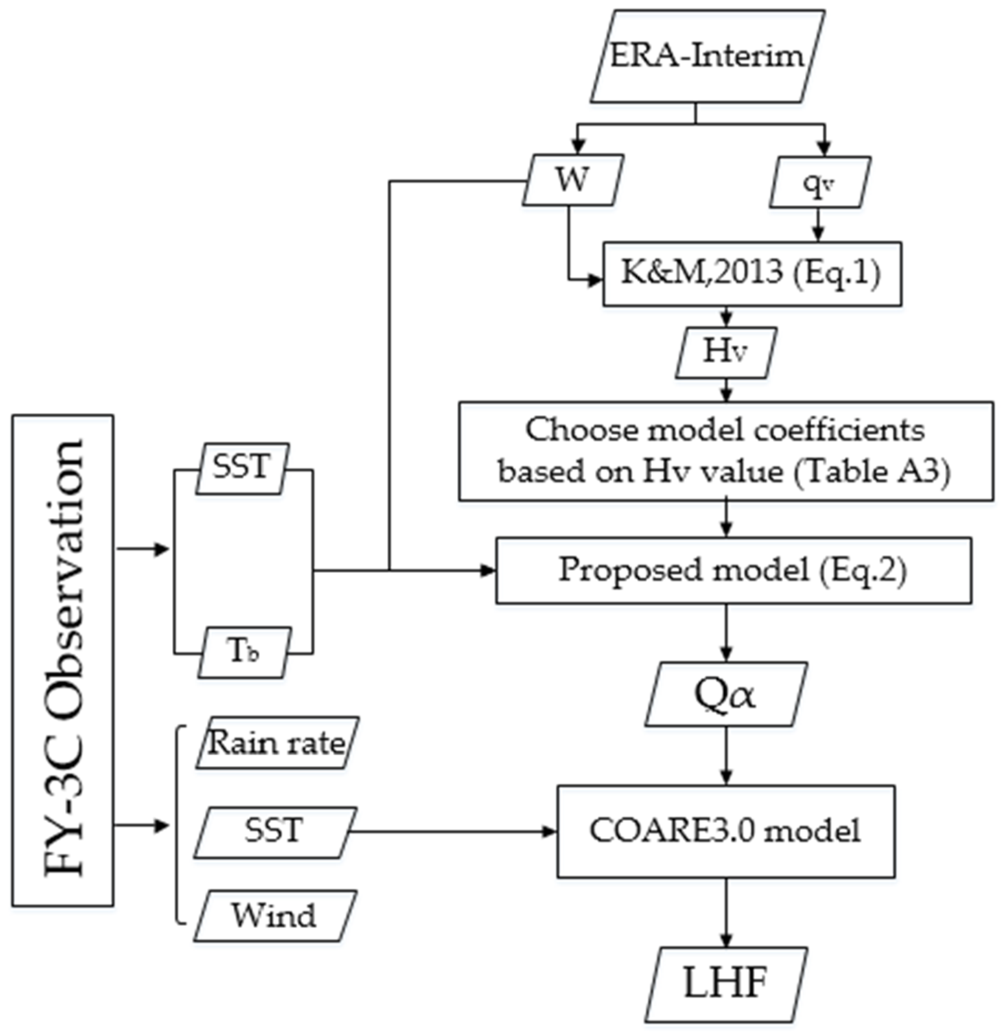
There are different satellite remote sensing algorithms for air-–sea specific humidity and LHF, but these algorithms do not fully consider the effects of SST, W, and vertical moisture structure on $Q_a$. In this study, a methodological framework was proposed to estimate $Q_a$ and LHF from FY-3C observations and meteorological auxiliary data (see Figure 1).

3.1. Relationship between SST and W

Kanemaru and Masunaga (2013) illustrated that the water vapor scale height ($H_v$) is a good indicator of the vertical moisture gradient between the boundary layer and the free troposphere,

$$H_v=\frac{\mathrm{W}}{{\rho }_a{q}_v},$$

(1)

where W is the column water vapor (kg/m²), ${\rho }_a$ is the density of dry air (1.2 kg/m³), and $q_v$ is the surface water vapor mixing ratio (g/kg) [33]. Here, values of W and $q_v$ were derived from ERA-Interim [32].

Tomita et al. (2018) presented the value of $H_v$ influencing the relationship between $Q_a$ and the brightness temperature. They proposed a method using additional data for $H_v$ as a proxy for the vertical moisture gradient to retrieve $Q_a$ beyond previous linear multi-regressions. The influence of W on $Q_a$ is considered in their method.

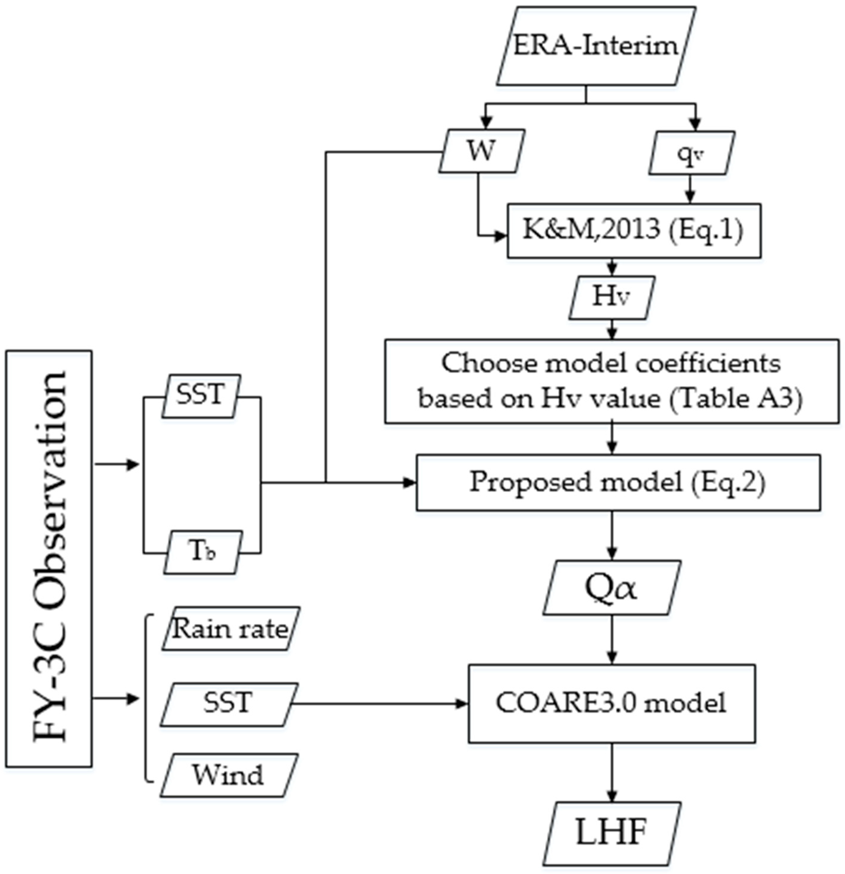
Kanemaru and Masunaga (2013) also found that the relationship between SST and W changes depending on the values of SST [33]. W shows contrasting sensitivities to SST depending on the SST. The SST–W relation resembles the C–C (Clausius–Clapeyron) relation [34,35] when SST is lower than 27 °C. For higher SST, the SST–W relation does not follow the Clausius–Clapeyron relation because the influence of W on $H_v$ is larger than the SST contribution. Hence, the SST should be considered when we study the relationship between W and $Q_a$.

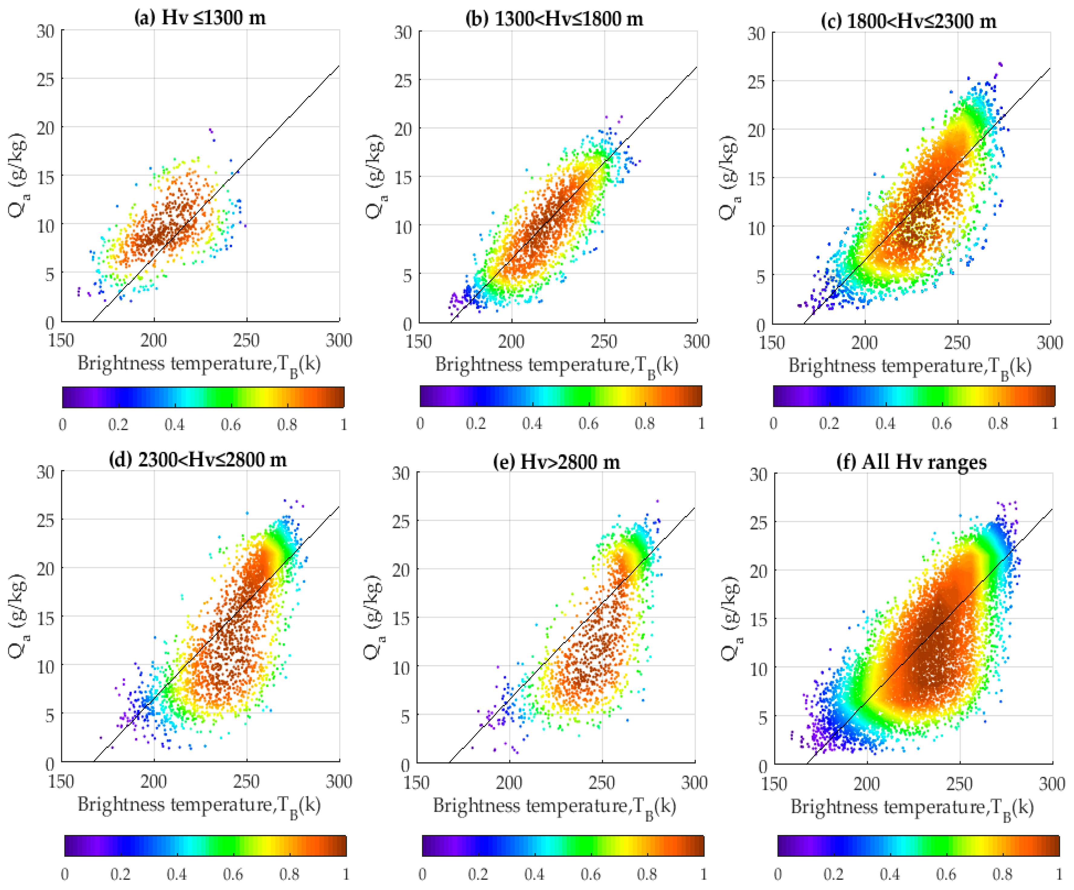
Figure 2a–e shows the relationship between the obtained SST and W with the change in $H_v$ values. The color depth represents the value of $q_v$. Five groups of $H_v$ (≤1300 m, 1300–1800 m, 1800–2300 m, 2300–2800 m, and >2800 m) were temporally averaged for the year 2014, using the data from 60° S to 60° N. Lower $H_v$ corresponded to relatively lower W values. For example, when $H_v$ ≤ 1300 m, the maximum value of W was less than 35 kg/m², while the maximum value reached 85 kg/m² if $H_v$ > 2800 m. This may be because lower $H_v$ corresponds to atmospheric columns containing moisture in relatively lower layers, and higher $H_v$ corresponds to columns containing moisture up to relatively higher layers [25].

Furthermore, compared with higher $H_v$ values, the increase ratio of $dW/dSST$ was smaller at lower $H_v$ values (see Figure 2). The ratio changed with SST, the thick line shows a cubic regression curve calculated from SST and W. Figure 2f shows the correlation between the increase ratio and the SST at each $H_v$ range. When the SST was lower than 27 °C, the increase ratio had less change with the increase of SST at lower $H_v$ ranges. When the SST was near 27 °C, the ratio of $dW/dSST$ was significantly increased (especially at higher $H_v$ ranges), and then the increase ratio was reduced. The influence of the SST–W relation on $Q_a$ will be further discussed in Section 3.2.

3.2. Channel Sensitivity

Figure 3 and Figure 4 show the relationship between $Q_a$ and the brightness temperature ($T_{B,23V}$ and $T_{B,89H}$) at five $H_v$ ranges. The brightness temperature dataset is from the FY-3C MWRI. The color depth indicates the density of data and the black line was calculated using all $H_v$ data. There was a basic positive linear relationship between brightness temperature and $Q_a$, and the $H_v$ values influenced this relationship. When the $H_v$ was small (Figure 3a–c, under 2300 m; Figure 4a,b, under 1800 m), the relationship appeared linear. However, the relationship between $Q_a$ and brightness temperature appeared to curve at higher $H_v$ ranges (Figure 3d and e, over 2300 m; Figure 4c–e, over 1800 m), which is similar to the results of Tomita et al. (2018) [25].

The basic relationship between $Q_a$ and the brightness temperature can be understood from the semi-linear relationship between W and the brightness temperature. $T_{B,23}$ and $T_{B,89}$ are well related to columnar water vapor [19,36]. When the value of W is large, the atmospheric column contains more water vapor [15]. This results in a higher brightness temperature due to higher microwave radiation from the increased amount of water vapor, so the basic relationship appears linear.

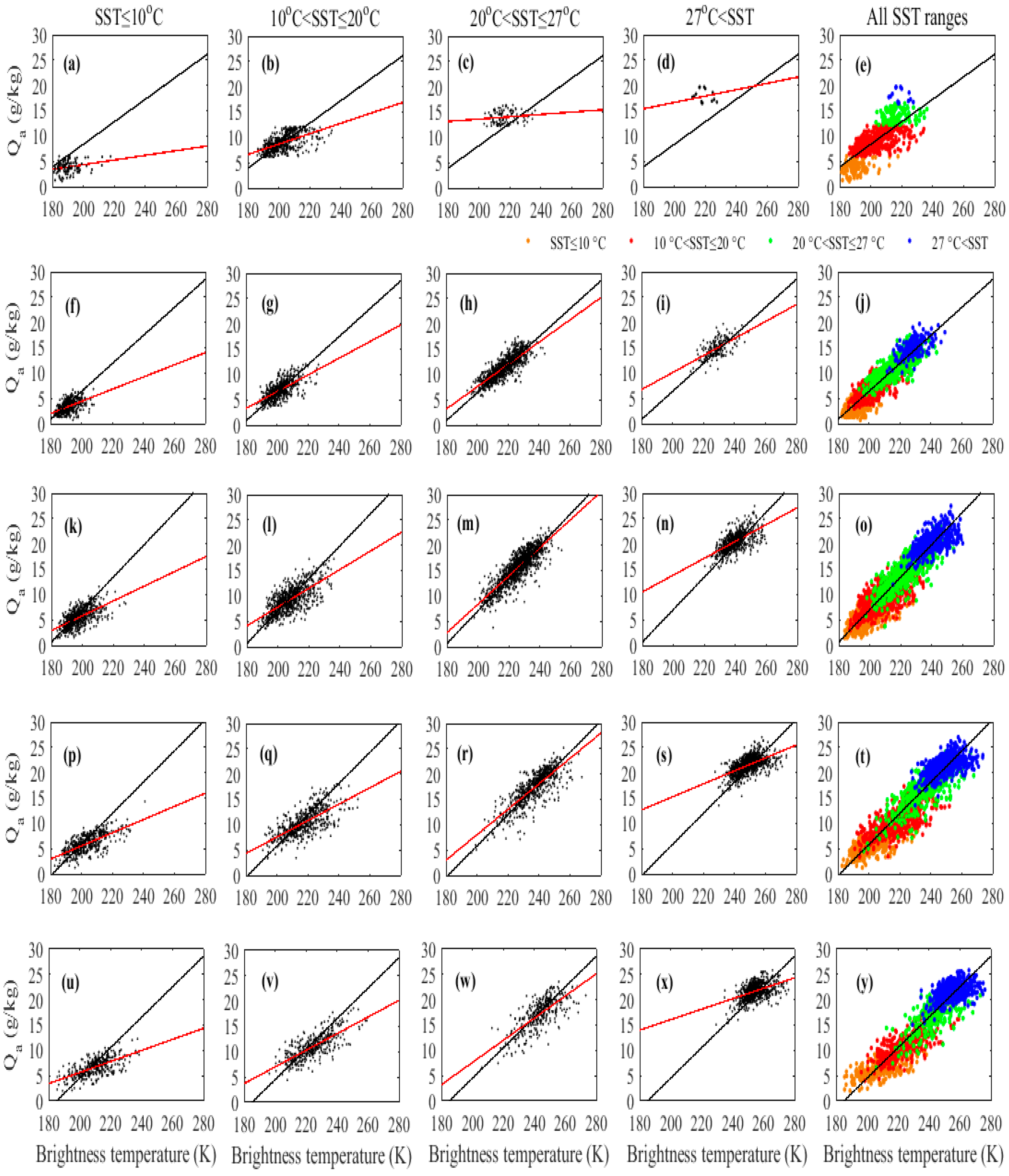
To further explore the effect of SST on the above phenomena, we divided the data shown in Figure 3 into four groups by SST. Figure 5 shows the relationship between brightness temperature (${\mathrm{T}}_{\mathrm{B},23\mathrm{V}}$), ${\mathrm{Q}}_{\mathrm{a}},$ and SST at each $H_v$ range. Red lines were calculated for each SST interval, and black lines were calculated using all data of each $H_v$ interval. Figure 5 demonstrates that the distribution of points is influenced by SST. In the SST ≤ 10 °C range, the slope of the scatter distribution was lower than the slope of all scatter data, and their difference was the largest in this interval. As the temperature increased, the difference between them decreased. Except for $H_v$ ≤ 1300 m, the range of 20–27 °C showed minimal difference, and then the difference increased again.

This phenomenon may be due to two reasons: (1) Difference in the amount of data between different temperature ranges has an impact on the results. For example, the ratio of the number of scatters in the range of 20–27 °C to the total number of scatters was the largest, which had a greater contribution to the slope of the fitting. In contrast, for the range of 0–10 °C and >27 °C the ratio was small and corresponded to a small contribution to the overall slope. (2) The linear relationship between $Q_a$ and $T_B$ was different at each SST range, which may be affected by the SST–W relation mentioned above. The difference in the effect of the SST increment on W further caused a change in the relationship between the $Q_a$ and $T_B$.

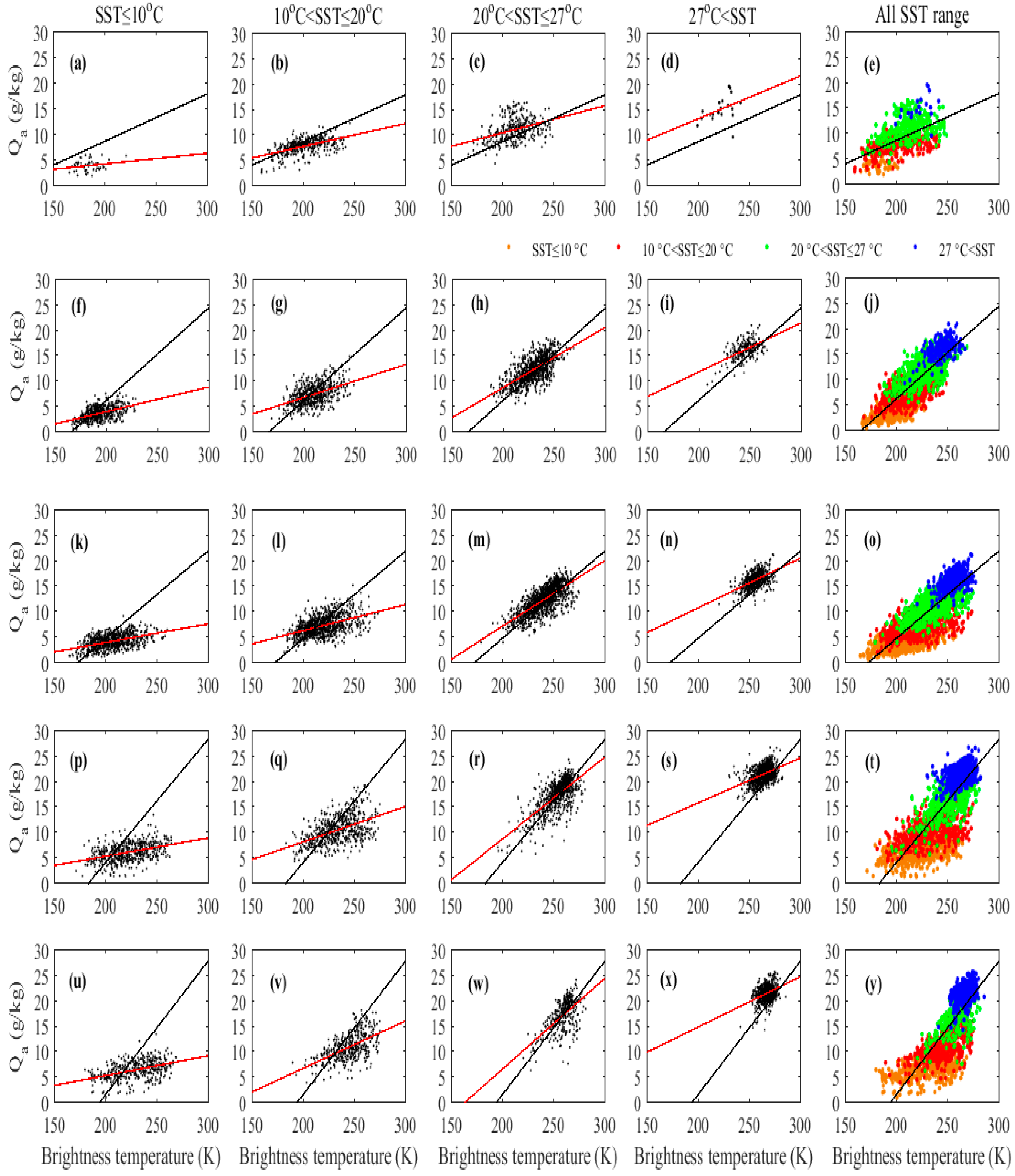
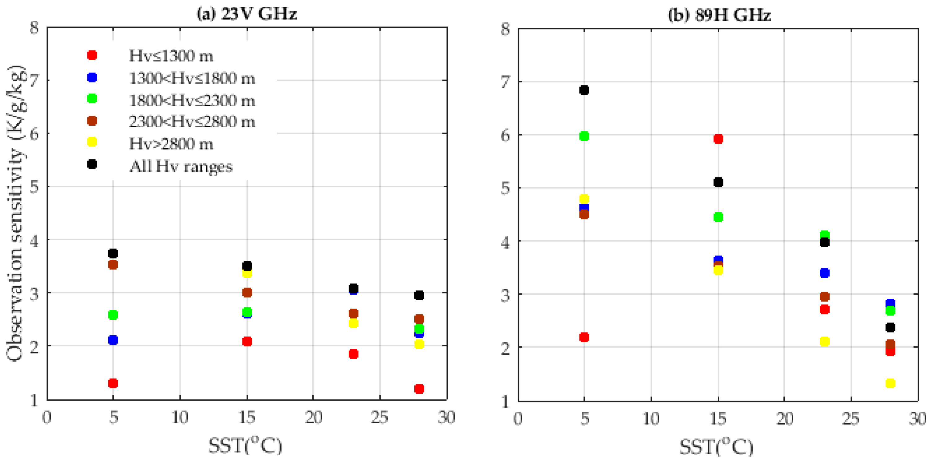
In the high frequency (89 H GHz) channel, we did the same analysis as shown in Figure 6. Compared with 23 V GHz, the scatters exhibited a more curvilinear relationship in the higher $H_v$ ranges. There was a significant difference in the relationship between $Q_a$ and $T_B$ in different SST ranges. We further used the observation sensitivity ($d{T}_B/d{Q}_a$) to analyze this phenomenon quantitatively, and the results are shown in Figure 7.

Figure 7 shows that the observation sensitivity varies with SST on the same $H_v$ range, and the relationship is affected by $H_v$ values. For the 23 V GHz channel, when $H_v$ ≤ 2300 m, the maximum value of observation sensitivity appeared in the mid-SST range, and there was minimal difference between different SST ranges. When $H_v$ > 2300 m, observation sensitivity gradually decreased with the increase of SST, which resulted in a curve distribution of scatters. In the 89 H GHz channel, there was a similar trend. When $H_v$ ≤ 1300 m, the maximum value of observation sensitivity appeared at 10–20 °C. Observation sensitivity decreased as SST increased when $H_v$ was larger than 1300 m. In addition, Figure 7 shows that the observation sensitivity value of 23 V GHz is lower than 89 H GHz channel as a whole. Furthermore, the variation amplitude between different SST ranges was lower than 89 H GHz. This difference has an effect on the relationship between $Q_a$ and $T_B$. Since the observation sensitivity is an inverse value of $d{Q}_a/d{T}_B$, the smaller variation of observation sensitivity in different SST ranges generates a closer relationship between $Q_a$ and $T_B$. Hence, the relationship appears linear at 23 V GHz radiation but appears curved at 89 H GHz. Higher $H_v$ values exhibit scatter points of both channels in the form of a curve. A similar result was found for the 23 H GHz and 89 V GHz observation channels, but was unclear for 10, 19, and 37 GHz channels.

In general, it was found that observation sensitivity within the same $H_v$ range changed depending on the value of SST. This trend may contribute to the curved relationship between $Q_a$ and $T_B$, particularly at higher $H_v$ values (Figure 5 and Figure 6). This result indicates that SST is an important parameter for $Q_a$ estimates and cannot be ignored. Previous algorithms based only on direct regression between $T_B$ and $Q_a$ might produce estimation errors for some ranges of SST.

3.3. Developed Algorithm

SST has been considered as an important near-surface meteorological parameter in some artificial intelligence algorithms when retrieving $Q_a$ and LHF [23,37]. From the relationship discussed in Section 3.1 and Section 3.2, we found clear connections between in situ $Q_a$ and $T_B$, and W was also useful because of its relationship with $Q_a$. In this study, an improved model was proposed based on the TO18 method. We suggested using all the brightness temperature data in order to obtain a more accurate estimation of the $Q_a$ (for more details of channel correlation and its impact on the regression please see Section 5 and Table A1). Moreover, because the relationship between $Q_a$ and $T_B$ appeared curved at higher $H_v$ ranges, the quadratic terms for $T_{B,23V/H}$ and $T_{B,89V/H}$ were used for inversion. Ultimately, the new regression equation had the following form:

$$\begin{array}{c}{Q}_a=c_0+c_1{T}_{B,10V}+c_2{T}_{B,10H}+c_3{T}_{B,19V}+c_4{T}_{B,19H}+c_5{T}_{B,23V}+c_6{T}_{B,23V}^2+c_7{T}_{B,23H}\\ +c_8{T}_{B,23H}^2+c_9{T}_{B,37V}+c_{10}{T}_{B,37H}+c_{11}{T}_{B,89V}+c_{12}{T}_{B,89V}^2+c_{13}{T}_{B,89H}+c_{14}{T}_{B,89H}^2\\ +c_{15}\mathrm{W}\cdot \mathrm{SST},\end{array}$$

(2)

where $Q_a$ denotes the specific air humidity at 10 m in g/kg, $T_B$ is the brightness temperature in Kelvin, SST is in °C, $c_{0–15}$ are regression coefficients, and the p-values for these retrieved coefficients are listed in

Table 2. p-Values of retrieved coefficients for different water vapor scale heights $H_v$ (m).

p-Values	${\mathit{H}}_{\mathit{v}} \le 1300$	$1300< {\mathit{H}}_{\mathit{v}}\le 1800$	$1800< {\mathit{H}}_{\mathit{v}}\le 2300$	$2300< {\mathit{H}}_{\mathit{v}}\le 2800$	$2800< {\mathit{H}}_{\mathit{v}}\le 3300$	${\mathit{H}}_{\mathit{v}} >3300$
C0	1.51 × 10−63	0.0000	0.0000	0.0000	0.0000	6.60 × 10−77
C1	3.27 × 10−15	4.71 × 10−69	6.58 × 10−94	5.12 × 10−141	0.0000	3.33 × 10−76
C2	2.41 × 10−06	8.39 × 10−227	2.40 × 10−59	4.94 × 10−152	0.0000	3.77 × 10−37
C3	0.532	9.67 × 10−125	0.0000	0.0000	0.0000	6.14 × 10−08
C4	4.02 × 10−11	1.68 × 10−363	0.0272	0.0010	8.81 × 10−22	0.2000
C5	1.04 × 10−06	0.0000	0.0000	0.0000	0.0000	5.22 × 10−132
C6	4.71 × 10−08	0.0000	0.0000	0.0000	0.0000	3.25 × 10−124
C7	1.17 × 10−13	0.0000	2.71 × 10−05	0.0000	0.0000	3.60 × 10−107
C8	3.86 × 10−05	0.0000	5.87 × 10−156	0.0000	0.0000	6.83 × 10−145
C9	1.53 × 10−42	3.38 × 10−56	6.78 × 10−15	8.98 × 10−06	6.73 × 10−17	0.0640
C10	1.10 × 10−09	0.0000	0.0000	3.65 × 10−45	4.90 × 10−88	9.94 × 10−19
C11	6.15 × 10−59	0.0000	0.0000	5.15 × 10−223	8.84 × 10−90	0.4254
C12	3.89 × 10−37	0.0000	1.10 × 10−226	0.0000	4.14 × 10−118	0.0214
C13	3.09 × 10−10	0.0000	0.0000	2.01 × 10−215	1.02 × 10−150	0.0070
C14	0.647	0.0000	2.93 × 10−141	0.0000	1.19 × 10−188	0.6800
C15	1.51 × 10−63	0.0000	0.0000	0.0000	0.0000	6.62 × 10−77

.

The p-values for regression coefficients indicate the significance in estimating the $Q_a$. A small p-value (<0.05) indicates that the regression is significant. Overall, we found that all input parameters were significant in the regression model (see Table 2). But there were some exceptions, which were related to different $H_v$ intervals. For example, when $H_v$ ≤ 1300 m, the p-values of $c_3$ and $c_{14}$ were larger than 0.05. In comparison, when 1300 m < $H_v$ ≤ 3300 m, all p-values were less than 0.05, representing very significant parameters in improved models. For $c_{14}$, the quadratic coefficient of $T_{B,89H}$ in extreme $H_v$ values (≤1300 m or >3300 m) was larger than 0.05. These demonstrate that in extremely large or very small $H_v$, the term was weakly correlated with retrieved results. In this study, we deleted the terms with p-values greater than 0.05 when obtaining the retrieved coefficients. Finally, the values of coefficients are listed in

Table A3. Regression coefficients of proposed model for different water vapor scale heights $H_v$ (m).

Coefficients	${\mathit{H}}_{\mathit{v}} \le 1300$	$1300< {\mathit{H}}_{\mathit{v}}\le 1800$	$1800< {\mathit{H}}_{\mathit{v}}\le 2300$	$2300< {\mathit{H}}_{\mathit{v}}\le 2800$	$2800< {\mathit{H}}_{\mathit{v}}\le 3300$	${\mathit{H}}_{\mathit{v}}>3300$
C0	−101.7520	−74.1441	−56.4953	−46.2155	−61.2600	−86.3314
C1	0.0252	−0.0103	−0.0149	−0.0089	−0.0725	−0.0519
C2	−0.0125	0.0093	0.0043	0.0021	0.0325	0.0183
C3	0.0000	−0.0110	−0.0404	−0.0725	−0.1106	−0.0247
C4	−0.0358	−0.0138	0.0105	0.0163	0.0418	0.0000
C5	−0.2015	0.1604	0.3649	0.6717	0.9174	1.1411
C6	0.0005	−0.0003	−0.0009	−0.0013	−0.0019	−0.0024
C7	0.1012	0.0548	0.0359	−0.1322	−0.2903	−0.3309
C8	−0.0002	−2.40 × 10−5	7.54 × 10−5	0.0004	0.0008	0.0010
C9	−0.0902	−0.0450	−0.0123	−0.0097	0.0684	0.0000
C10	0.0235	−0.0264	−0.0228	−0.0029	−0.0442	−0.0223
C11	0.9919	0.5658	0.2115	−0.1695	−0.2098	0.0000
C12	−0.0016	−0.0010	−0.0003	0.0005	0.0005	8.82 × 10−5
C13	−0.0743	−0.0805	−0.0282	0.1024	0.1952	−0.0173
C14	0.0000	0.0001	1.12 × 10−5	−0.0003	−0.0005	0.0000
C15	0.0180	0.0121	0.0097	0.0074	0.0071	0.0061

.

The LHF is widely estimated using the COARE3.0 bulk aerodynamic formula [30], which is suitable for both satellite and in situ data. The LHF can be expressed as follows:

$$LHF={\rho }_a{C}_{e}U{L}_e(Q_a-Q_s),$$

(3)

where $C_e$ is the turbulent exchange coefficient for latent heat flux, $L_e$ is the latent heat of evaporation, and $Q_s$ is surface humidity. $U$ and $Q_a$ are the wind speed and specific air humidity relative to the sea surface at the height of 10 m.

In this study, $Q_a$ was estimated using satellite data and $U$ was derived from FY-3C MWRI orbit products. $Q_s$ was calculated from SST assuming saturation at the surface, where a multiplier factor of 0.98 was used when considering the reduction in vapor pressure caused by a typical salinity of 34 psu. $C_e$ was computed by the COARE3.0 algorithm, which was mainly influenced by conditions of light wind, stable stratification, sea spray, and other sea-state information. In addition, FY-3C MWRI orbit products of rain rate were used as input data to estimate LHF. Detailed information of these products can be obtained from the website: http://www.nsmc.org.cn/en/NSMC/Home/Index.html.

4. Experimental Results

4.1. Evaluation with In Situ Data

4.1.1. Air Specific Humidity

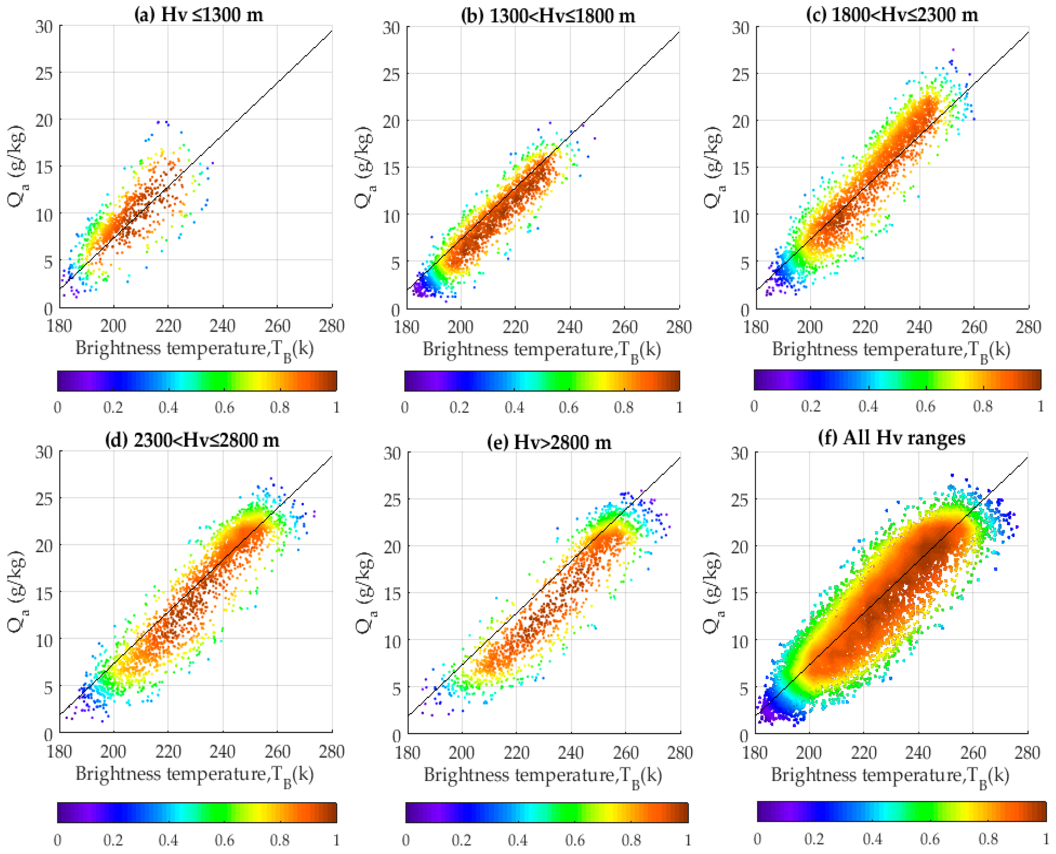
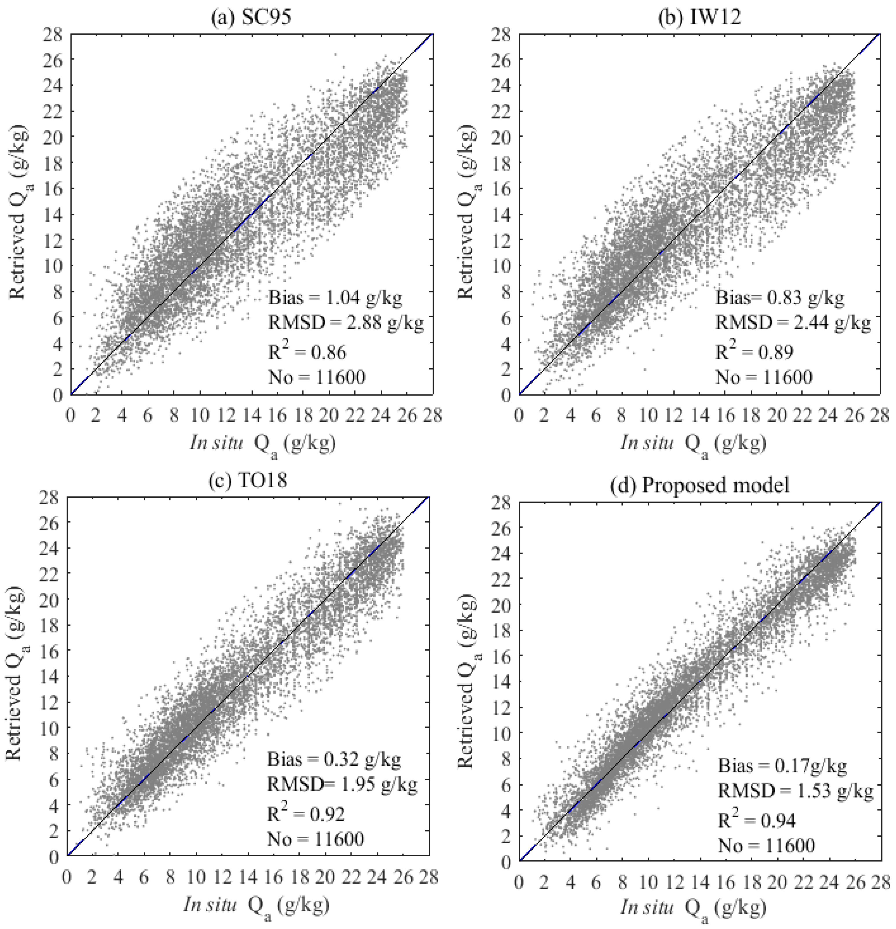
In this section, satellite-derived $Q_a$ fields were compared with in situ observed $Q_a$. We also compared the proposed model with three other existing empirical algorithms (SC95, IW12, and TO18). Details of these four $Q_a$ retrieval algorithms are given in

Table 3. Channels and meteorological parameters for each algorithm.

Algorithm	10 GHz	19 GHz	23 GHz	37 GHz	89 GHz	Parameters
SC95		19 V/H	23 V	37 V/H
IW12		19 V/H	23 V	37 V/H	89 V/H
TO18	10 V/H	19 V/H	23 V/H	37 V/H	89 V/H	W
Proposed model	10 V/H	19 V/H	23 V/H	37 V/H	89 V/H	W and SST

SC95: Schlüssel et al. (1995); IW12: Iwasaki et al. (2012); and TO18: Tomita et al. (2018).

.

Figure 8 shows scatter plots of the comparison of in situ observed $Q_a$ with four satellite-derived $Q_a$ values (the Sample 2 data). The proposed model has good performance, with a root mean square difference (RMSD) of 1.53 g/kg, and a correlation coefficient (R²) of 0.94. TO18 has an RMSD and R² of the order of 1.95 g/kg and 0.92, respectively. SC95 has an RMSD and R² of 2.88 g/kg, and 0.86, respectively. IW12 performed better (RMSD, 2.44 g/kg; R², 0.89) than SC95 due to the use of the high-frequency 89 GHz channel.

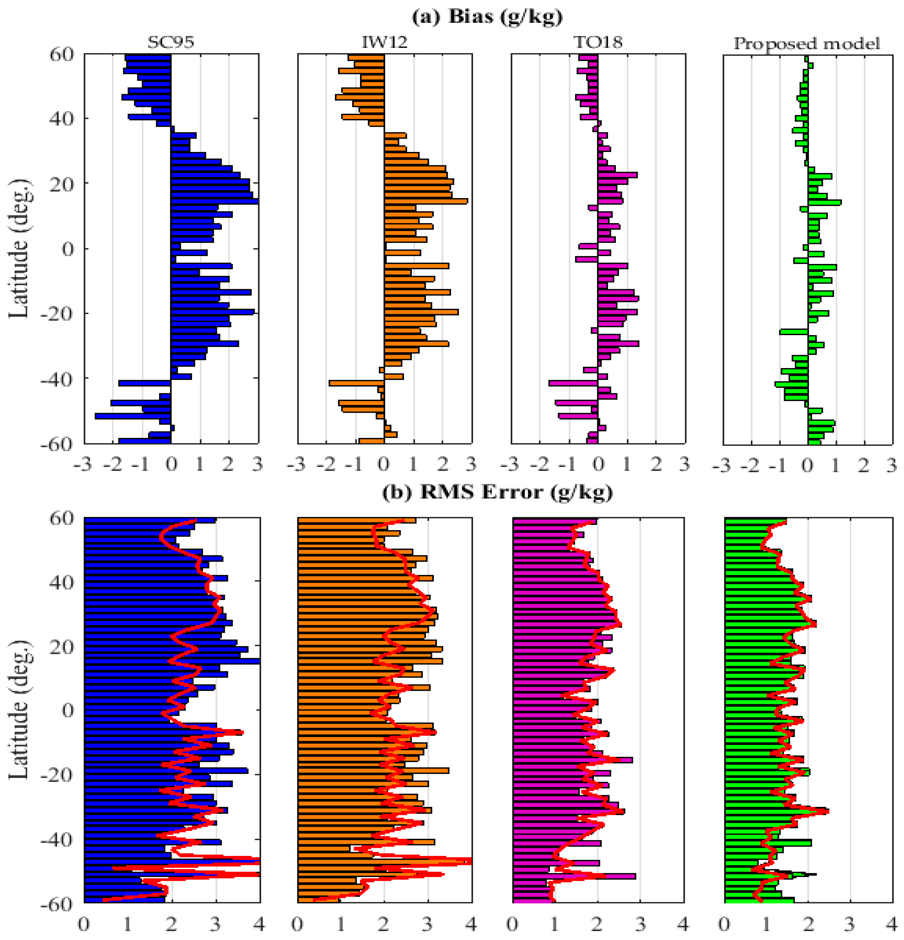
Figure 9 shows the zonal averages of the bias (satellite derived $Q_a$ minus in situ $Q_a$), RMSD, and standard deviation difference (SDD) for the Sample 2 data. For the proposed model, the RMSD are less than 2.0 g/kg and biases are less than 1 g/kg over most of the latitudes. The bias (Figure 9a) for all algorithms tends to show positive values, especially in low and mid-latitude regions. This means that all four algorithms tend to overestimate $Q_a$. Compared with the other three algorithms, the proposed model’s $Q_a$ shows the smallest bias. The accuracy of satellite-derived $Q_a$ was significantly improved by using SST.

4.1.2. Latent Heat Flux

To assess the improvement resulting from the proposed $Q_a$ model on satellite-derived LHF, the satellite-derived LHF was compared with in situ LHF, which was calculated from in situ measurements (i.e., Sample 2 data).

Table 4. Comparisons between satellite and in situ data for the four algorithms.

Statistics	Specific Air Humidity			Latent Heat Flux
	Bias (g/kg)	RMSD (g/kg)	Correlation (R2)	Bias (W/m2)	RMSD (W/m2)	Correlation (R2)
SC95
45°–60° N 45°–60° S	−1.34	2.46	0.85	−26.50	39.24	0.48
15°–45° N 15°– 45° S	0.66	3.16	0.81	14.10	51.96	0.51
15° S–15° N	1.72	2.96	0.70	34.98	48.14	0.49
IW12
45°–60° N 45°– 60° S	−1.16	2.29	0.86	−22.76	36.54	0.49
15°–45° N 15°–45° S	0.53	2.98	0.84	11.89	48.84	0.55
15° S–15° N	1.41	2.41	0.74	28.74	42.61	0.54
TO18
45°– 60° N 45°– 60° S	−0.48	1.57	0.93	−16.18	31.87	0.63
15°– 45° N 15°–45° S	0.15	2.20	0.90	10.98	44.14	0.75
15° S–15° N	0.44	1.83	0.82	8.45	35.50	0.70
Proposed model
45°–60° N 45°–60° S	−0.14	1.11	0.95	−12.89	23.44	0.72
15°–45° N 15°–45° S	0.08	1.76	0.92	2.40	34.24	0.87
15° S–15° N	0.24	1.51	0.86	4.87	29.05	0.82

provides some statistical results of these comparisons. The statistics were averaged in the high (45°–60° N, 45°–60° S), mid (15°–45° N, 15°–45° S), and low (15° S–15° N) latitudinal regions.

Compared with the other three existing algorithms, the proposed method had good performance in estimating LHF. There were significant statistical improvements of LHF due to these improvements of $Q_a$. For example, in mid-latitude regions, the bias, RMSD, and R² for SC95 method were 0.66 g/kg, 3.16 g/kg, and 0.81, respectively, while those of the proposed model were 0.08 g/kg, 1.76 g/kg and 0.92, respectively. Corresponding parameters of LHF (SC95) were 14.10 W/m², 51.96 W/m², and 0.51, while those of the proposed model were 2.40 W/m², 34.24 W/m², and 0.87, respectively. The differences between satellite and in situ data were dependent on zonal locations, which were mainly influenced by the accuracy of $Q_a$.

4.2. ${\mathrm{Q}}_{\mathrm{a}}$ Comparison with NOAA CIRES Datasets

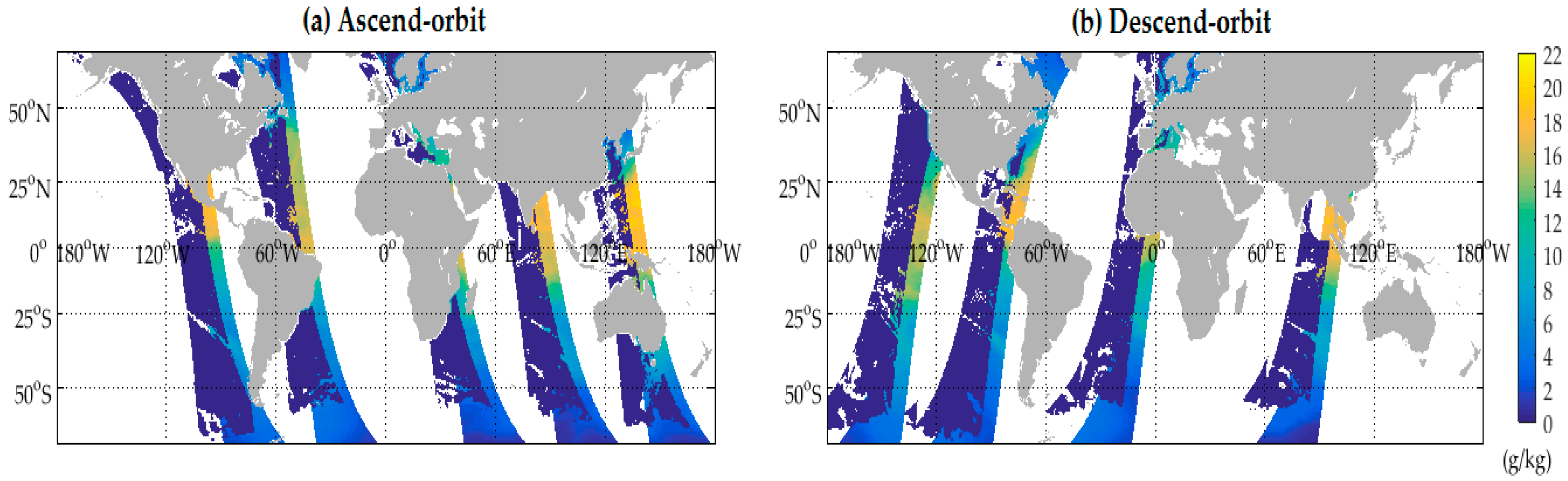
The satellite-derived $Q_a$ fields were also compared with NOAA CIRES Multi-Satellite Humidity. To match up two $Q_a$ datasets, we set criteria that the temporal and spatial differences had to be less than 180 min and 25 km, respectively. Figure 10 shows the two datasets covering the common area on 6 October 2014.

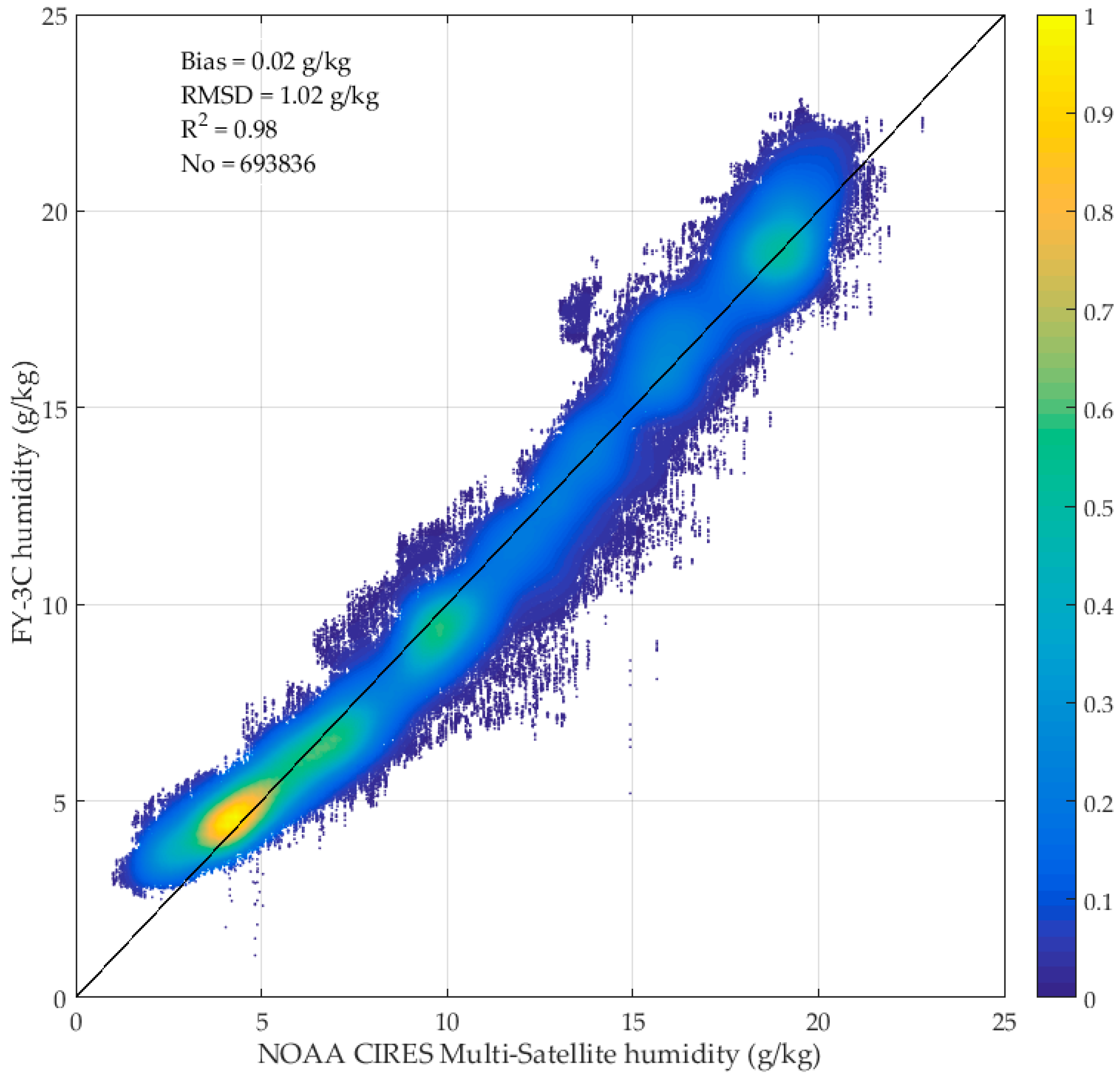
Figure 11 shows the results of the comparison between NOAA CIRES Multi-Satellite Humidity and FY-3C humidity (total 693,836 collocated data) on 6 October 2014. Compared with the Multi-Satellite $Q_a$ dataset, the $Q_a$ derived from FY-3C satellite had a bias, RMSD, and R² of 0.02 g/kg, 1.02 g/kg, and 0.98, respectively.

5. Discussion

In this study, we investigated the observation sensitivity ($d{T}_B/d{Q}_a$) variation with the SST at different $H_v$ ranges (as described in Section 3.2). This phenomenon indicates that previous $Q_a$ algorithms based only on direct regression between brightness temperature and $Q_a$ might not be accurate enough for some SST and humidity conditions.

Hence, we introduced the SST as a key input parameter into $Q_a$ estimation (Equation (2)). Radiations from 10 microwave channels of the FY-3C satellite were all used in the proposed algorithm. It is well known that $T_B$ with the same frequency but different polarizations, has a strong correlation. The Pearson correlation coefficients also clearly show that there are strong dependencies between some channels used in Equation (2) (Table A1). To better show the importance of each indicator in the proposed model, a stepwise regression was used (

Table A2. Stepwise regression analysis for predicting the specific air humidity (Q_a).

Model	Adjusted R Square	Residual Mean Square	F-Test
			F	df1	df2	Sig. F Change
1 *	0.897	2.544367	104,793.588	1	11,598	0.000
2	0.922	1.933543	708,22.499	1	11,597	0.000
3	0.928	1.774980	51,823.867	1	11,596	0.000
4	0.930	1.636417	42,380.563	1	11,595	0.000
5	0.935	1.488377	37,518.207	1	11,594	0.000
6	0.940	1.428013	32,669.545	1	11,593	0.000
7	0.942	1.399309	28,620.837	1	11,592	0.000
8	0.943	1.394626	25,140.234	1	11,591	0.000
9	0.944	1.382297	22,546.893	1	11,590	0.000
10	0.944	1.378660	20,621.421	1	11,589	0.000
11	0.945	1.361343	19,567.475	1	11,588	0.000

* 1: Constant, WSST; 2: Constant, WSST, B9; 3. Constant, WSST, B9, B10; 4: Constant, WSST, B9, B10, B5; 5: Constant, WSST, B9, B10, B5, B7; 6: Constant, WSST, B9, B10, B5, B7, B6; 7: Constant, WSST, B9, B10, B5, B7, B6, B8; 8: Constant, WSST, B9, B10, B5, B7, B6, B8, B4; 9: Constant, WSST, B9, B10, B5, B7, B6, B8, B4, B1; 10: Constant, WSST, B9, B10, B5, B7, B6, B8, B4, B1, B2; 11: Constant, WSST, B9, B10, B5, B7, B6, B8, B4, B1, B2, B3.

). The results of the stepwise regression show that when the number of parameters used in the regression model was larger than six, the improvements of R² and residual mean square of the regression model were very small. However, it was also shown that including more channels could improve the proposed linear model, even if the newly added channel was highly correlated to existing channels. Besides, we regressed the model coefficients according to different $H_v$ ranges. In order to obtain the best fitness of the regression model, we chose to include all channels in the proposed model. Moreover, we decided to use quadratic terms for $T_{B,23V/H}$ and $T_{B,89V/H}$ because the relationship between $Q_a$ and brightness temperature appears curved at higher $H_v$ ranges. These measures ensure a superior output of our model for different humidity conditions in the global oceans.

It is worth mentioning that the original SC95, IW12, and TO18 algorithms were derived from different training data and may not be well suited for the FY-3C MWRI instrument. Thus, we derived new regression coefficients for three algorithms before using them to compare with the proposed method. Figure 8 shows that the proposed method has the lowest RMSD (1.53 g/kg) and the highest R² (0.94). In addition, satellite-derived $Q_a$ were also compared with the NOAA CIRES Multi-Satellite humidity dataset, their bias, RMSD, and R² were 0.02 g/kg, 1.02 g/kg, and 0.98, respectively. These comparison results indicate that adding SST as an input parameter can improve $Q_a$ and LHF estimation. There are regional differences of the outputs of the proposed model. The RMSD of $Q_a$ in mid-latitude regions (15°–45° N, 15°–45° S) was 1.76 g/kg, and the RMSD of high (45°–60° N, 45°–60° S) and low (15° S–15° N) latitude regions were 1.11 and 1.51 g/kg, respectively. This difference may result from the SST–W relation. Kanemaru and Masunaga (2013) concluded that the W is closely related with SST and dependent on regional position [33].

We obtained SST data from the FY-3C MWRI orbit products and $H_v$ data from atmospheric reanalysis. Therefore, any potential error and dependency for either variable may affect the accuracy of $Q_a$. Furthermore, the training and testing dataset of in situ measurements was collected from the global sea area between 60° S and 60° N. This means that the proposed $Q_a$ model is also only valid for these regions. Although we believe that the form of this algorithm is universal in calculating global specific humidity, the retrieved coefficients are only available for FY-3C MWRI. For other space-borne radiometers, these coefficients need to be recalculated.

6. Conclusions

Latent heat flux represents an important aspect of the atmosphere–ocean interaction. Additionally, satellite-derived specific humidity has been a major source of error for the estimation of LHF. In order to improve the estimation accuracy of specific humidity, we proposed a new $Q_a$ model based on FY-3C microwave brightness temperature observations. We found the relationship of observation sensitivity ($d{T}_B/d{Q}_a$) changed depending on the range of SST, especially at larger $H_v$, so SST was added into the estimation model. This improved model gives better estimates of $Q_a$ and LHF when compared with three existing methods (SC95, IW12, and TO18). The satellite-derived $Q_a$ were also compared with in situ data, and their bias, RMSD, and R² were 0.17 g/kg, 1.53 g/kg, and 0.94, respectively. The satellite $Q_a$ were also compared with NOAA CIRES $Q_a$ datasets, with a bias, RMSD, and R² of 0.02 g/kg, 1.02 g/kg, and 0.98, respectively. The differences between satellite LHF and in situ LHF were dependent on zonal locations: In high latitude regions (45°–60° N, 45°–60° S), the bias, RMSD, and R² were 12.89 W/m², 23.44 W/m², and 0.72, respectively; in mid-latitude regions (15°–45° N, 15°–45° S), the bias, RMSD, and R² were 2.4 W/m², 34.24 W/m², and 0.87, respectively; in low latitude regions (15° S–15° N), the bias, RMSD, and R² were 4.87 W/m², 29.05 W/m², and 0.82, respectively, which were mainly influenced by the accuracy of $Q_a$ (see Table 4).

As shown in the study, SST as an additional input parameter greatly improved the estimation accuracy of $Q_a$ and LHF for the FY-3C satellite observation. The innovative aspect of the algorithm was based on the finding of a relationship between SST, W, and water vapor profile information, which provided a theoretical basis for satellite-derived $Q_a$ and LHF. Furthermore, SST and W were directly used as input parameters for estimating $Q_a$. Both variables may introduce unknown redundant information to model outputs. Future work should explore the essence of the SST–W relationship and improve the simulation method of the vertical moisture structure.

References

- Gulev, S.K.; Latif, M.; Keenlyside, N.; Park, W.; Koltermann, K.P. North atlantic ocean control on surface heat flux on multidecadal timescales. Nature 2013, 499, 464–467. [Google Scholar] [CrossRef] [PubMed]
- Dutra, E.; Stepanenko, V.M.; Balsamo, G.; Viterbo, P.; Miranda, P.M.A.; Mironov, D.; Schar, C. An offline study of the impact of lakes on the performance of the ecmwf surface scheme. Boreal Environ. Res. 2010, 15, 100–112. [Google Scholar]
- Woolway, R.I.; Verburg, P.; Lenters, J.D.; Merchant, C.J.; Hamilton, D.P.; Brookes, J.; de Eyto, E.; Kelly, S.; Healey, N.C.; Hook, S.; et al. Geographic and temporal variations in turbulent heat loss from lakes: A global analysis across 45 lakes. Limnol. Oceanogr. 2018, 63, 2436–2449. [Google Scholar] [CrossRef]
- Bourassa, M.A.; Gille, S.T.; Bitz, C.; Carlson, D.; Cerovecki, I.; Clayson, C.A.; Cronin, M.F.; Drennan, W.M.; Fairall, C.W.; Hoffman, R.N.; et al. High-latitude ocean and sea ice surface fluxes: Challenges for climate research. Bull. Am. Meteorol. Soc. 2013, 94, 403–423. [Google Scholar] [CrossRef]
- Bunker, A.F. Computations of surface-energy flux and annual air-sea interaction cycles of north-atlantic ocean. Mon. Weather Rev. 1976, 104, 1122–1140. [Google Scholar] [CrossRef]
- Hasse, L.; Smith, S.D. Local sea surface wind, wind stress, and sensible and latent heat fluxes. J. Clim. 1997, 10, 2711–2724. [Google Scholar] [CrossRef]
- Bentamy, A.; Piolle, J.F.; Grouazel, A.; Danielson, R.; Gulev, S.; Paul, F.; Azelmat, H.; Mathieu, P.P.; von Schuckmann, K.; Sathyendranath, S.; et al. Review and assessment of latent and sensible heat flux accuracy over the global oceans. Remote Sens. Environ. 2017, 201, 196–218. [Google Scholar] [CrossRef]
- Andersson, A.; Fennig, K.; Klepp, C.; Bakan, S.; Grassl, H.; Schulz, J. The hamburg ocean atmosphere parameters and fluxes from satellite data—Hoaps-3. Earth Syst. Sci. Data 2010, 3, 143–194. [Google Scholar] [CrossRef]
- Andersson, A.; Klepp, C.; Fennig, K.; Bakan, S.; Grassl, H.; Schulz, J. Evaluation of hoaps-3 ocean surface freshwater flux components. J. Appl. Meteorol. Climatol. 2011, 50, 379–398. [Google Scholar] [CrossRef]
- Kubota, M.; Iwasaka, N.; Kizu, S.; Kondo, M.; Kutsuwada, K. Japanese ocean flux data sets with use of remote sensing observations (j-ofuro). J. Oceanogr. 2002, 58, 213–225. [Google Scholar] [CrossRef]
- Shie, C.L.; Chiu, L.S.; Adler, R.; Nelkin, E.; Lin, I.I.; Xie, P.P.; Wang, F.C.; Chokngamwong, R.; Olson, W.; Chu, D.A. A note on reviving the goddard satellite-based surface turbulent fluxes (gsstf) dataset. Adv. Atmos. Sci. 2009, 26, 1071–1080. [Google Scholar] [CrossRef]
- Bentamy, A.; Grodsky, S.A.; Katsaros, K.; Mestas-Nunez, A.M.; Blanke, B.; Desbiolles, F. Improvement in airsea flux estimates derived from satellite observations. Int. J. Remote Sens. 2013, 34, 5243–5261. [Google Scholar] [CrossRef]
- Tomita, H.; Kubota, M.; Cronin, M.F.; Iwasaki, S.; Konda, M.; Ichikawa, H. An assessment of surface heat fluxes from j-ofuro2 at the keo and jkeo sites. J. Geophys. Res. Oceans 2010, 115. [Google Scholar] [CrossRef]
- Liu, W.T.; Niiler, P.P. Determination of monthly mean humidity in the atmospheric surface-layer over oceans from satellite data. J. Phys. Oceanogr. 1984, 14, 1451–1457. [Google Scholar] [CrossRef]
- Liu, W.T. Statistical relation between monthly mean precipitable water and surface-level humidity over global oceans. Mon. Weather Rev. 1986, 114, 1591–1602. [Google Scholar] [CrossRef]
- Schulz, J.; Schluessel, P.; Grassl, H. Water-vapor in the atmospheric boundary layer over oceans from ssm/i measurements. Int. J. Remote Sens. 1993, 14, 2773–2789. [Google Scholar] [CrossRef]
- Schlussel, P.; Schanz, L.; Englisch, G. Retrieval of latent-heat flux and longwave irradiance at the sea-surface from ssm/i and avhrr measurements. In Satellite Monitoring of the Earth’s Surface and Atmosphere; Arnault, S., Ed.; Pergamon Press Ltd: Oxford, UK, 1995; Volume 16, pp. 107–116. [Google Scholar]
- Bentamy, A.; Katsaros, K.B.; Mestas-Nunez, A.M.; Drennan, W.M.; Forde, E.B.; Roquet, H. Satellite estimates of wind speed and latent heat flux over the global oceans. J. Clim. 2003, 16, 637–656. [Google Scholar] [CrossRef]
- Iwasaki, S.; Kubota, M. Algorithms for estimation of air-specific humidity using tmi data. Int. J. Remote Sens. 2012, 33, 7413–7430. [Google Scholar] [CrossRef]
- Jackson, D.L.; Wick, G.A.; Bates, J.J. Near-surface retrieval of air temperature and specific humidity using multisensor microwave satellite observations. J. Geophys. Res. Atmos. 2006, 111. [Google Scholar] [CrossRef]
- Jackson, D.L.; Wick, G.A.; Robertson, F.R. Improved multisensor approach to satellite-retrieved near-surface specific humidity observations. J. Geophys. Res. Atmos. 2009, 114. [Google Scholar] [CrossRef]
- Jones, C.; Peterson, P.; Gautier, C. A new method for deriving ocean surface specific humidity and air temperature: An artificial neural network approach. J. Appl. Meteorol. 1999, 38, 1229–1245. [Google Scholar] [CrossRef]
- Singh, R.; Joshi, P.C.; Kishtawal, C.M. A new technique for estimation of surface latent heat fluxes using satellite-based observations. Mon. Weather Rev. 2005, 133, 2692–2710. [Google Scholar] [CrossRef]
- Roberts, J.B.; Clayson, C.A.; Robertson, F.R.; Jackson, D.L. Predicting near-surface atmospheric variables from special sensor microwave/imager using neural networks with a first-guess approach. J. Geophys. Res. Atmos. 2010, 115. [Google Scholar] [CrossRef]
- Tomita, H.; Hihara, T.; Kubota, M. Improved satellite estimation of near-surface humidity using vertical water vapor profile information. Geophys. Res. Lett. 2018, 45, 899–906. [Google Scholar] [CrossRef]
- Yang, J.; Zhang, P.; Lu, N.M.; Yang, Z.D.; Shi, J.M.; Dong, C.H. Improvements on global meteorological observations from the current fengyun 3 satellites and beyond. Int. J. Digit. Earth 2012, 5, 251–265. [Google Scholar] [CrossRef]
- Freeman, E.; Woodruff, S.D.; Worley, S.J.; Lubker, S.J.; Kent, E.C.; Angel, W.E.; Berry, D.I.; Brohan, P.; Eastman, R.; Gates, L.; et al. Icoads release 3.0: A major update to the historical marine climate record. Int. J. Climatol. 2017, 37, 2211–2232. [Google Scholar] [CrossRef]
- Buck, A.L. New equations for computing vapor-pressure and enhancement factor. J. Appl. Meteorol. 1981, 20, 1527–1532. [Google Scholar] [CrossRef]
- Wilks, D.S. Statistical Methods in the Atmospheric Sciences, 2nd ed.; Academic Press: San Diego, CA, USA, 2006; 627p. [Google Scholar]
- Fairall, C.W.; Bradley, E.F.; Hare, J.E.; Grachev, A.A.; Edson, J.B. Bulk parameterization of air-sea fluxes: Updates and verification for the coare algorithm. J. Clim. 2003, 16, 571–591. [Google Scholar] [CrossRef]
- Jackson, D.L.; Wick, G.A. Near-surface air temperature retrieval derived from amsu-a and sea surface temperature observations. J. Atmos. Ocean. Technol. 2010, 27, 1769–1776. [Google Scholar] [CrossRef]
- Dee, D.P.; Uppala, S.M.; Simmons, A.J.; Berrisford, P.; Poli, P.; Kobayashi, S.; Andrae, U.; Balmaseda, M.A.; Balsamo, G.; Bauer, P.; et al. The era-interim reanalysis: Configuration and performance of the data assimilation system. Q. J. R. Meteorol. Soc. 2011, 137, 553–597. [Google Scholar] [CrossRef]
- Kanemaru, K.; Masunaga, H. A satellite study of the relationship between sea surface temperature and column water vapor over tropical and subtropical oceans. J. Clim. 2013, 26, 4204–4218. [Google Scholar] [CrossRef]
- Stephens, G.L. On the relationship between water-vapor over the oceans and sea-surface temperature. J. Clim. 1990, 3, 634–645. [Google Scholar] [CrossRef]
- Jackson, D.L.; Stephens, G.L. A study of ssm/i-derived columnar water-vapor over the global oceans. J. Clim. 1995, 8, 2025–2038. [Google Scholar] [CrossRef]
- Grody, N.C. Remote-sensing of atmospheric water-content from satellites using microwave radiometry. IEEE Trans. Antennas Propag. 1976, 24, 155–162. [Google Scholar] [CrossRef]
- Singh, R.; Joshi, P.C.; Kishtawal, C.M.; Pal, P.K. A new method for estimation of near surface specific humidity over global oceans. Meteorol. Atmos. Phys. 2006, 94, 1–10. [Google Scholar] [CrossRef]
Figure 1.
Methodological framework to estimate global air–sea and latent heat flux (LHF) using FY-3C satellite observations.
Figure 2.
(a–e) The relationship between sea surface temperature (SST), column water vapor (W), and surface water vapor mixing ratio (g/kg, color) on different ranges of water vapor scale height (m). Each figure shows a cubic regression curve calculated from SST and W. (f) SST compared to increase ratio (W/SST, kg/m2·°C) over five ranges, calculated from daily data and averaged from the range of 60° S to 60° N.
Figure 3.
Scatter diagrams showing the relationship between , and , using the Sample 1 data. (a) For ≤ 1300 m; (b) for 1300 m < ≤ 1800 m; (c) for 1800 m < ≤ 2300 m; (d) for 2300 m < ≤ 2800 m; (e) for > 2800 m; and (f) for all ranges. Each figure shows a linear regression line calculated using all range data. Color depth indicates the density of data.
Figure 4.
Figure 5.
The relationship between , and SST. (a–e) For ≤ 1300 m; (f–j) for 1300 m < ≤ 1800 m; (k–o) for 1800 m < ≤ 2300 m; (p–t) for 2300 m < ≤ 2800 m; and (u–y) for > 2800 m. Each subfigure shows a linear regression black line calculated using all data of the same range; the red line was calculated using the corresponding SST range data.
Figure 6.
Figure 7.
SST compared with observation sensitivity from a linear fitting for each SST range. (a) For 23 V GHz and (b) for 89 H GHz.
Figure 8.
Comparisons between in situ observed and four satellite-derived values (g/kg). (a) For SC95; (b) for IW12; (c) for TO18; and (d) for the proposed model.
Figure 9.
Zonal distributions of the comparative statistics between in situ observed and satellite-derived values for four algorithms, including (a) averaged bias, (b) root mean square difference (RMSD), and standard deviation difference (SDD, plotted as red lines). Statistics were averaged for each 2° bias.
Figure 10.
The common coverage area of NOAA CIRES Multi-Satellite Humidity (dark blue strip) and FY-3C humidity (colored strip) on 6 October 2014. Color depth indicates the value of specific air humidity. (a) Ascending orbit and (b) descending orbit.
Figure 11.
Results of the comparison between NOAA CIRES Multi-Satellite Humidity and FY-3C humidity on 6 October 2014. Color depth indicates the density of data.