Article

Comparison of Satellite and UAV-Based Multispectral Imagery for Vineyard Variability Assessment

1
Dipartimento di Elettronica e Telecomunicazioni (DET), Politecnico di Torino, Corso Duca degli Abruzzi 24, 10129 Torino, Italy
2
Dipartimento Energia (DENERG), Politecnico di Torino, Corso Duca degli Abruzzi 24, 10129 Torino, Italy
3
Dipartimento di Scienze Agrarie, Forestali e Alimentari (DiSAFA), Università degli Studi di Torino, Largo Paolo Braccini 2, 10095 Grugliasco (TO), Italy
*
Author to whom correspondence should be addressed.
Remote Sens. 2019, 11(4), 436; https://doi.org/10.3390/rs11040436
Submission received: 14 January 2019 / Revised: 12 February 2019 / Accepted: 17 February 2019 / Published: 20 February 2019

Abstract

:
In agriculture, remotely sensed data play a crucial role in providing valuable information on crop and soil status to perform effective management. Several spectral indices have proven to be valuable tools in describing crop spatial and temporal variability. In this paper, a detailed analysis and comparison of vineyard multispectral imagery, provided by decametric resolution satellite and low altitude Unmanned Aerial Vehicle (UAV) platforms, is presented. The effectiveness of Sentinel-2 imagery and of high-resolution UAV aerial images was evaluated by considering the well-known relation between the Normalised Difference Vegetation Index (NDVI) and crop vigour. After being pre-processed, the data from UAV was compared with the satellite imagery by computing three different NDVI indices to properly analyse the unbundled spectral contribution of the different elements in the vineyard environment considering: (i) the whole cropland surface; (ii) only the vine canopies; and (iii) only the inter-row terrain. The results show that the raw s resolution satellite imagery could not be directly used to reliably describe vineyard variability. Indeed, the contribution of inter-row surfaces to the remotely sensed dataset may affect the NDVI computation, leading to biased crop descriptors. On the contrary, vigour maps computed from the UAV imagery, considering only the pixels representing crop canopies, resulted to be more related to the in-field assessment compared to the satellite imagery. The proposed method may be extended to other crop typologies grown in rows or without intensive layout, where crop canopies do not extend to the whole surface or where the presence of weeds is significant.

Graphical Abstract

1. Introduction

Over the last two decades, precision agriculture (PA) has received significant attention in the agricultural community [1,2]. In viticulture, addressing difficulties during the production cycles by defining appropriate crop management, the PA approach has the final aim to improve vineyard yield and grape quality while reducing waste, costs and environmental impact [3,4].
A proper knowledge of the spatial variability between and within crop parcels is considered as a key factor for vine growers to estimate the outcomes in terms of yield and quality [5,6,7]. In this context, remote sensing (RS) has already proved its potential and effectiveness in spatiotemporal vegetation monitoring [8,9,10,11]. Indeed, data provided by optical sensors of multispectral and hyperspectral imagery systems are profitably exploited to compute a wide set of indices (such as the wide dynamic range vegetation index, the normalised difference red-edge index Index, etc.) by properly describing several crop biophysical characteristics [12,13]. In the PA domain, an additional effective application is found for within-field zone management, such as for sink size estimations [14,15] and soil moisture evaluations [16,17], with particular attention to automatic procedures [18,19,20]. Among the wide set of defined spectral indices, the normalized difference vegetation index (NDVI) is one of the most extensively used, since it is strictly related to crop vigour and, thus, to the estimated quality and quantity of field production [21,22,23,24,25].
Satellite multispectral imageries (MSI), due to sensors features and platforms altitude, covers extensive areas. In addition, many satellite programmes (such as Landsat, Modis, Aster, SPOT, Sentinel-1 and Sentinel-2) are nowadays providing free datasets, thus promoting satellite imagery exploitation for many agricultural applications [26,27,28,29,30], even with the multi-sensor data fusion approach [31]. Examples of valuable research contributions are the low-resolution Modis and high-resolution IKONOS satellite imagery exploitation for mapping vineyard leaf area [23,32]. Sentinel-2 offers decametric resolution in terms of space and time, with a ground sample distance (GSD) of up to 10 m and a revisit time of six days. Misregistration of sentinel-2A imageries was addressed in the Processing Baseline (version 02.04), and deployed by European Space Agency (ESA) on 15 June 2016 [33]. The effectiveness of decametric resolution satellite imagery in describing crop status and variability, particularly when applied to arable crops, forests and extensive plantations, has been proven by several relevant studies [12,34,35].
However, when considering crops with discontinuous layouts, such as vineyards and orchards, remote sensing becomes more challenging [36]. Indeed, the presence of inter-row paths and weed vegetation within the cropland may deeply affect the overall spectral indices computation, leading to a biased crop status assessment. Indeed, novel approaches and algorithms using Unmanned Aerial Vehicle (UAV) or satellite based multispectral imaging have been developed for vegetation pixels classification [37,38,39]. Low altitude platforms, such as UAV and airborne sensors, by providing imagery with a high spatial resolution (even a few centimetres) and a flexible flight scheduling [40], allow differentiating between pure canopy pixel and other objects in the scene [41,42,43,44,45] or even to classify different details within canopies [46,47,48].
In this paper, a detailed analysis and comparison of vineyards MSI, provided by a decametric resolution satellite and low altitude UAV platforms, is presented. The effectiveness of the MSI from Sentinel-2 and from the UAV airborne sensors, with very high resolution, was evaluated by considering the well-known relation between the NDVI and crop vigour. In particular, the paper is structured as follows: Section 2 reports information on the considered study area, on data acquisition from the satellite and the UAV platforms, and on the performed data processing to allow a comparison of the NDVI computed from different imagery sources. The results obtained by the data processing and comparison are discussed in Section 3. Section 4 reports the conclusions and future developments.

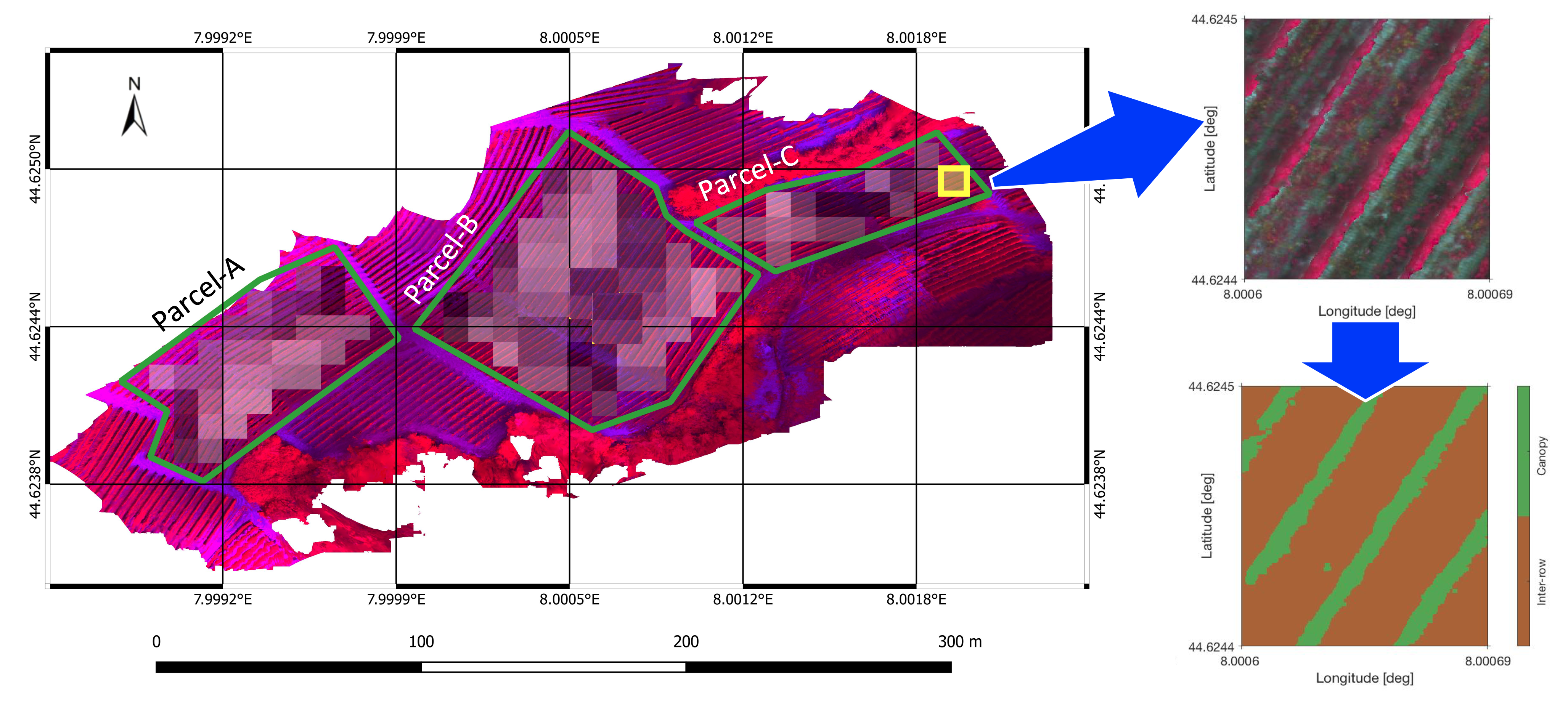
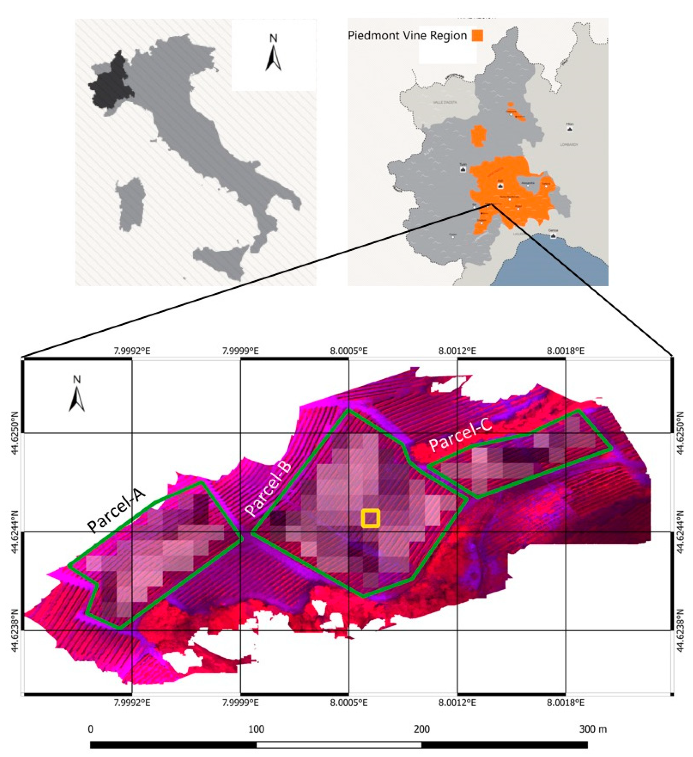
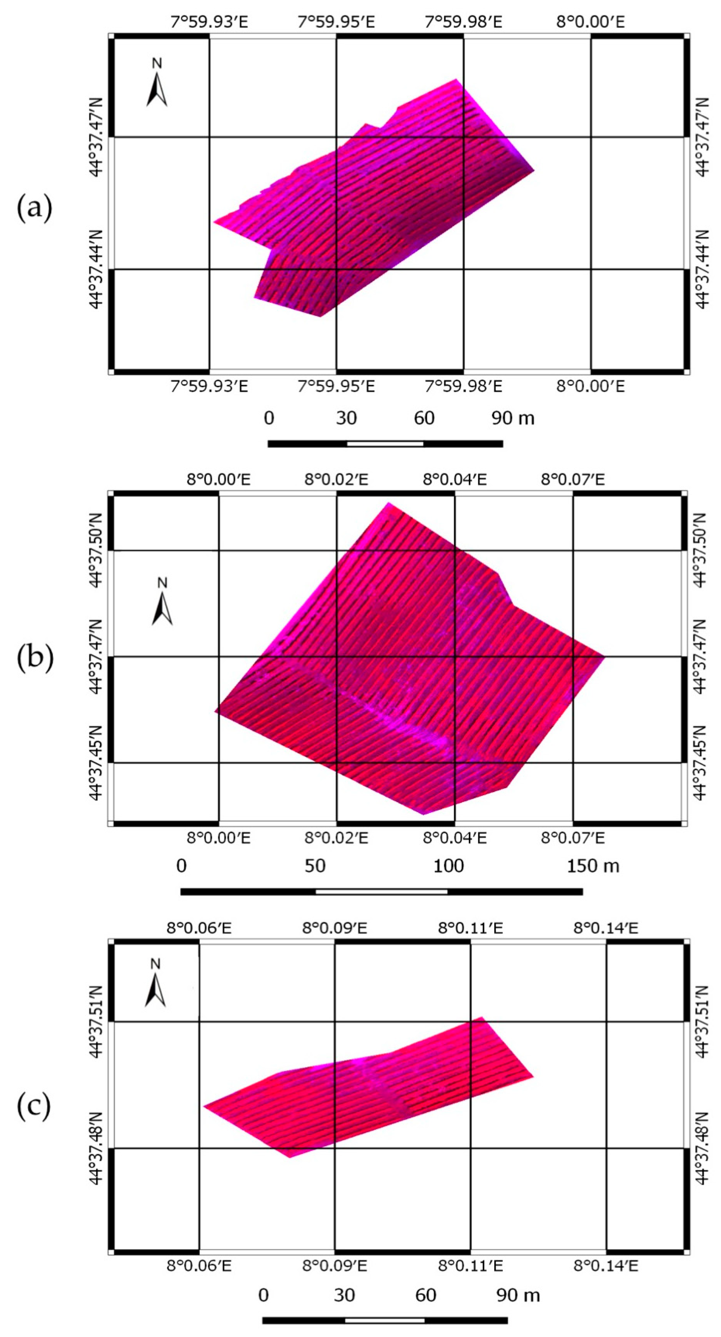
2. Materials and Methods

A vineyard located in Serralunga d’Alba (Piedmont, northwest of Italy), covering a surface of about 2.5 ha, was selected as a field test. The cropland, whose latitude and longitude positions range between [ 44.62334 ° 44.62539 ° ] and [ 7.99855 ° 8.00250 ° ] (World Geodetic System 1984-WGS84), includes three vineyard parcels (named “Parcel A”, “Parcel B” and “Parcel C”) cultivated with the cv Nebbiolo grapevine, with an area of around 0.36, 0.69 and 0.19 ha, respectively (Figure 1).
The vineyard is on a sloped land conformation, with an elevation ranging from 330 to 420 m above sea level and a predominantly southwest orientation. Due to the irregularity of the terrain morphology in terms of altitude and soil properties, the selected vineyard is characterised by a great variation in vine vigour within and between parcels. To extend the study to several vine phenological phases, the acquisition campaigns were performed from April to September 2017. Indeed, vigour varies during the phenological cycle from its minimum, after bud break (April), to its peak in the central part of the season (June–July). Finally, vigour decreases during the final phase of grape ripening. According to the crop stages defined in the BBCH-scale [49], the acquisitions were performed in Stages 57 (inflorescences fully developed), 77 (berries beginning to touch), 85 (softening of berries) and 89 (berries ripe for harvest). The meteorological course in the 2017 season was not aligned to the average temperature and rainfall trends of the region. In particular, March temperature values above the seasonal average led the vine buds to break about 15 days early. A sudden decrease in temperatures in the second half of April caused plant stress (frost damage) in some vines, slowing the vegetative growth of the plants. The phases of flowering and of fruit set, partially influenced by this phenomenon, occurred 10–15 days early. The total rainfall in the 2017 season was 480 mm, much lower than the average of the last 12 years (about 800 mm). This affected grape ripening particularly during August and September, months in which it is refined and completed. The reduced water availability partially contributed in accelerating ripening and in anticipating the veraison and the commercial harvest by about 10 days.

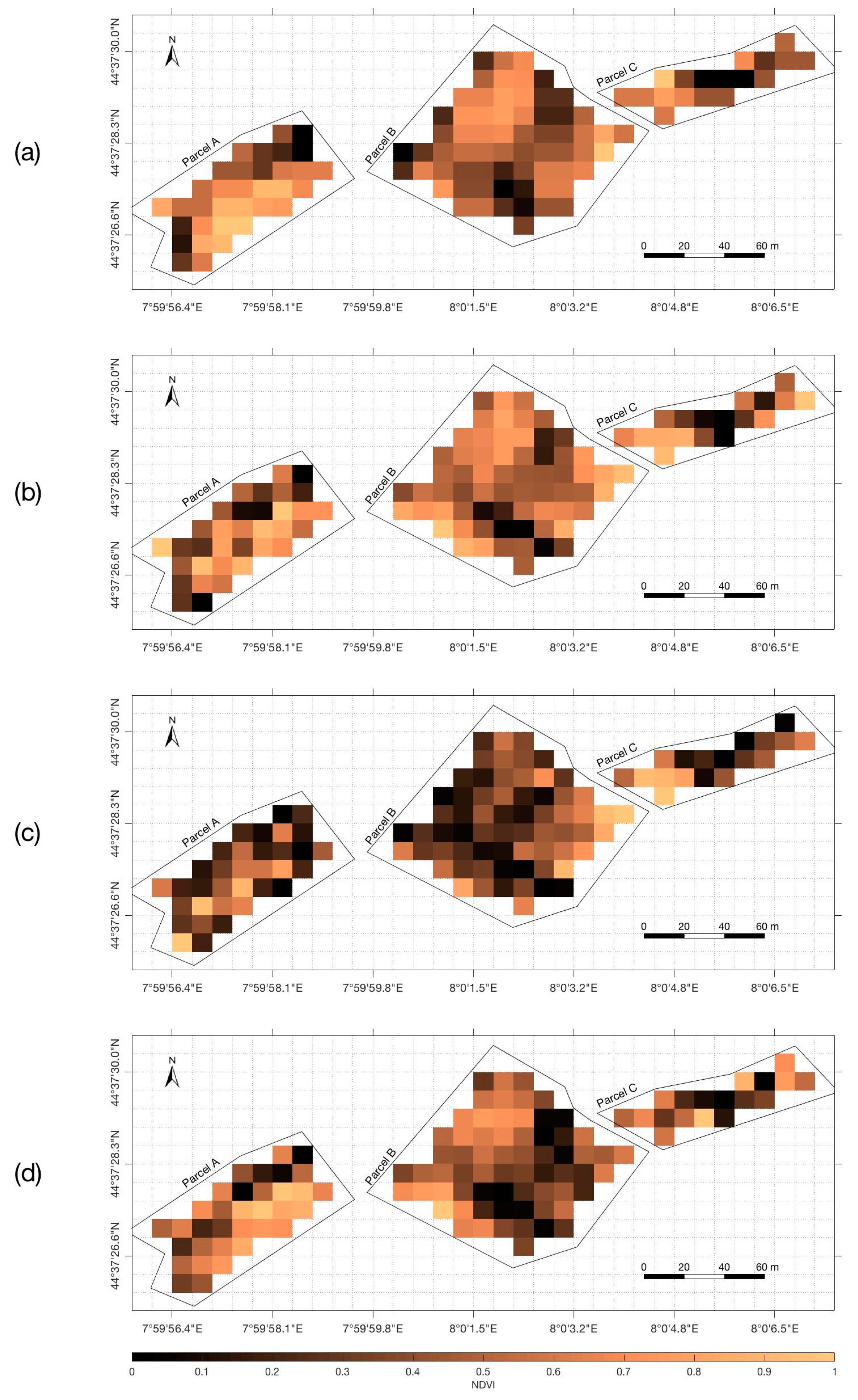
2.1. Satellite Time Series Images

The Sentinel-2 satellite is equipped with a multi-spectral imaging sensor that measures Earth’s Top of Atmosphere (TOA) reflected radiance in 13 spectral bands ranging from 443 nm to 2190 nm. The technical details of Sentinel-2 along with its spatial resolution and spectral ranges are summarised in Table 1. The Sentinel-2 imagery database, processed at different levels, can be downloaded from [50]. In this study, cloud-free level-2A Sentinel-2 Bottom of Atmosphere (BOA) reflectance images were used. The Level-2A imagery was derived from Level 1 by applying scene classification, atmospheric and BDRF correction algorithms, using SNAP toolbox (6.0) and sen2core processor (2.5.5) provided by the ESA [51,52,53,54]. Additional details about the Sentinel-2 MSI products can be found in [55].
The selected satellite tiles were acquired on four dates during the 2017 growing season (Table 2) to consider different vegetative vine statuses. Only red and near infrared bands (bands 4 and 8, respectively) were used in this study. The pixels completely included within the boundaries of the three considered “Parcel A”, “Parcel B” and “Parcel C” were selected, as shown in Figure 1. All relevant information regarding the satellite imagery processed in this study is organised and summarised in Table 1 and Table 2.

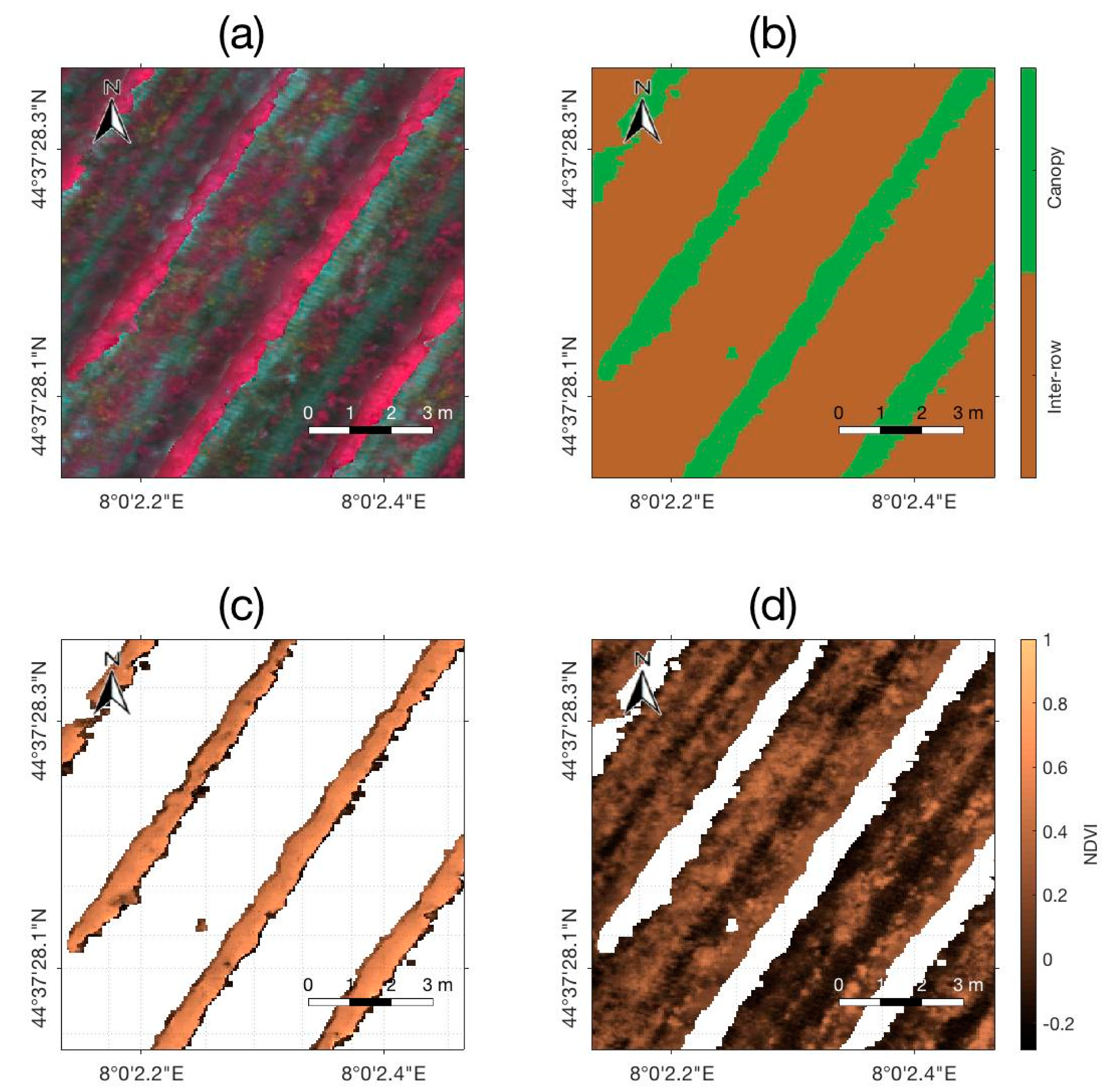
2.2. UAV-Based Imagery

The UAV-based MSI were generated with the Agisoft PhotoScan® software (Agisoft©, 2018 [56]) processing imagery blocks of more than 1000 aerial images acquired with an airborne Parrot Sequoia® multispectral camera (Parrot© SA, 2017 [57]). The UAV path was planned to maintain the flight height close to 35 m with respect to the terrain by properly defining waypoint sets for each mission block on the drone guidance platform on the base of the GIS cropland map. With this specification, the aerial images GSD resulted to be 5 cm (Figure 2).
A camera geometric calibration procedure was performed before the image alignment task; moreover, a radiometric calibration was applied to the image blocks by using the reference images of a Micasense calibrated reflectance panel [58] acquired before and after each UAV flight. A set of 12 ground control points, whose positions were determined with a differential GNSS system (with an accuracy of 0.1 m), was placed on selected vine trellis poles within the vineyard to georeference the MSI in a geodetic coordinates frame.
The UAV flights were performed on four different dates over the 2017 crop season (15 May, 29 June, 1 August and 23 September), according to the satellite visiting dates (Table 2).

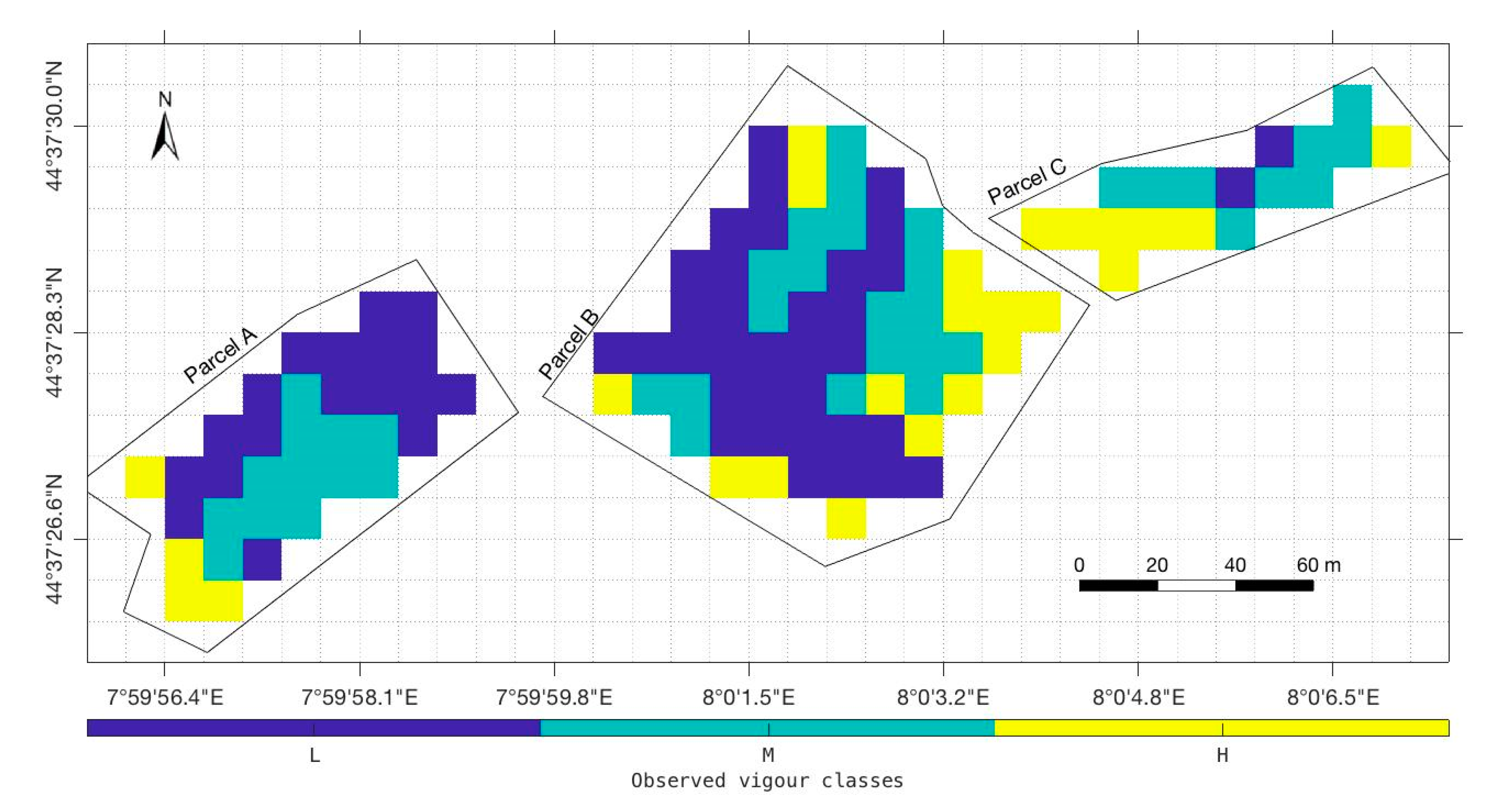
2.3. In-Field Vigour Assessment

The vigour of the vines within the three considered parcels in the study site was evaluated based on the results of a specific in-field survey performed by trained operators and on the past experience of the farmer. In the considered study site, the vigour variability is mainly related to the pedological soil conformation and to the water availability, since irrigation is not allowed by Piedmont regulation. The vigour classification was performed by defining three classes: low “L”, medium “M” and high “H”. A specific data processing was performed to make the in-field vigour assessment comparable to decametric resolution imagery. In particular, a 10 m × 10 m map was obtained by rastering and clustering a vector GIS map provided by expert agronomists made by a set of three vigour class layers, according to Sentinel-2 pixel location.

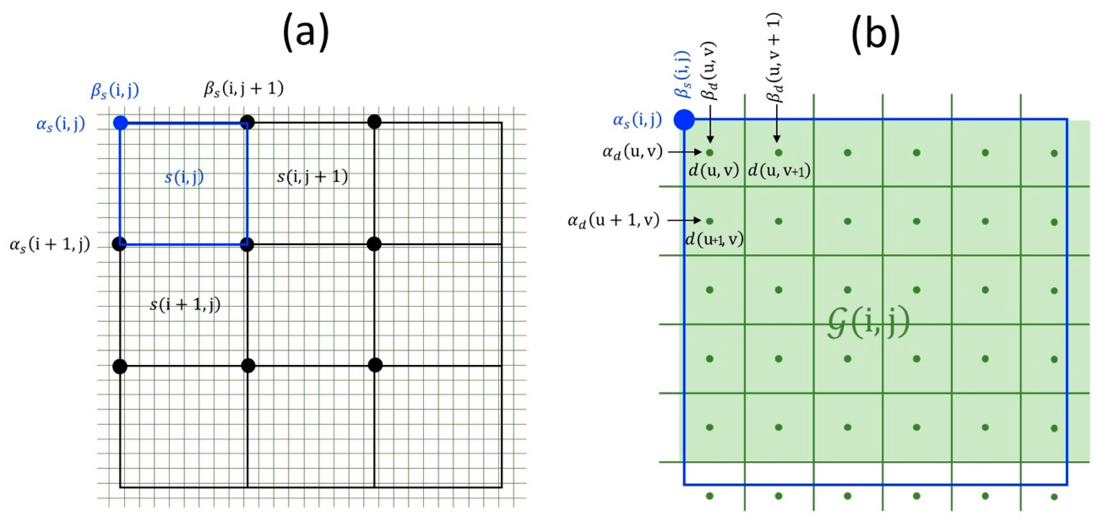
2.4. Data Processing
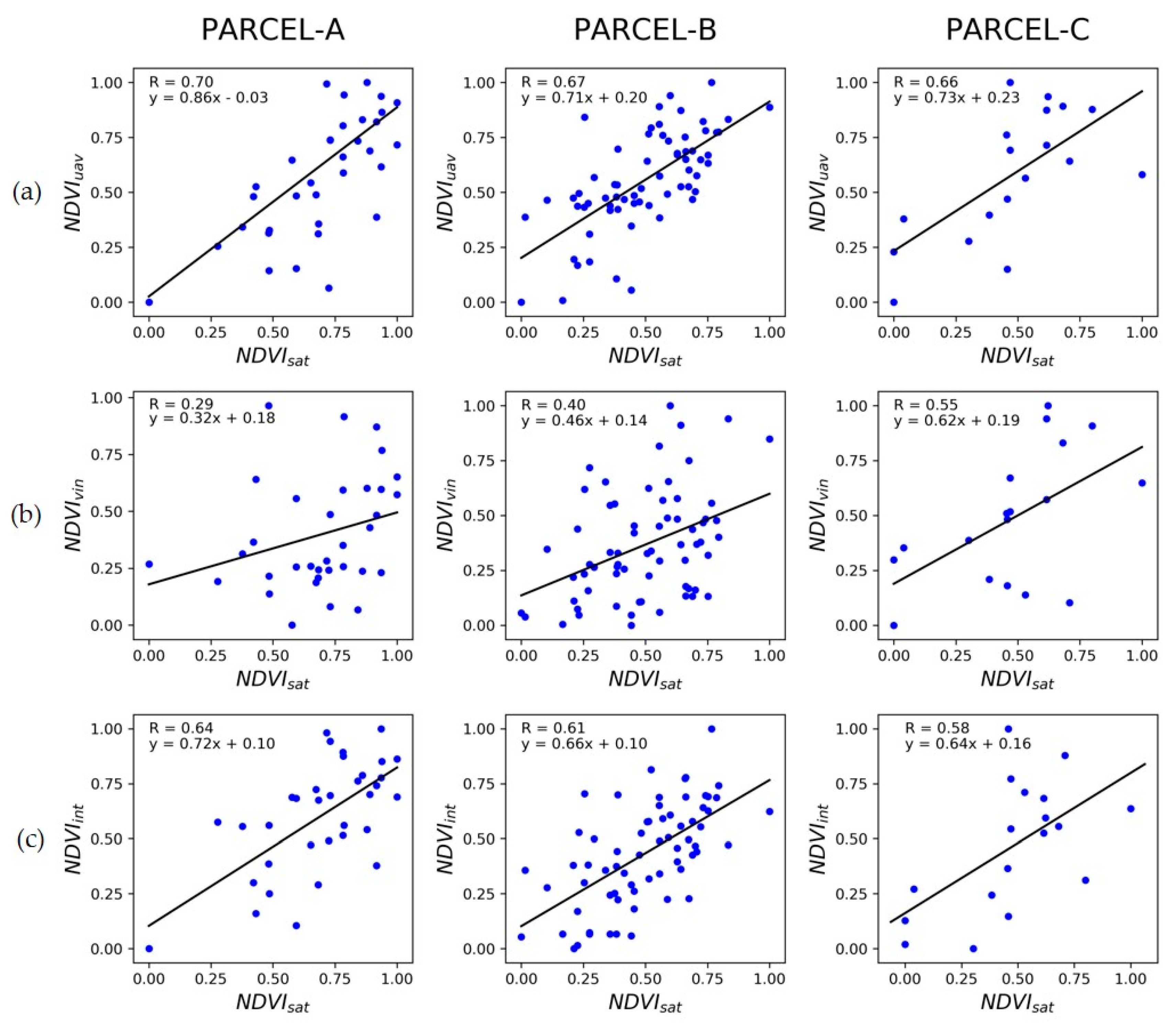
In this section, specific methods for data processing, developed to compare and investigate the imagery derived from the two platforms with different spatial resolutions, are presented and discussed in detail.
A tile S , derived from the satellite platform, can be considered as an ordered grid of pixels s ( i , j ) , with indices i and j representing the pixel row and column locations in the raster matrix, respectively. Each pixel s ( i , j ) was here defined as s ( i , j ) = [ α s ( i , j ) , β s ( i , j ) , n R ( i , j ) , n N ( i , j ) ] T S , where α s ( i , j ) and β s ( i , j ) are the latitude and longitude coordinates (expressed in WGS84) of the upper left corner of pixel s ( i , j ) , respectively, and n R ( i , j ) and n N ( i , j ) are the pixel digital numbers in the red and near infrared bands (12 bit representation), respectively.
Data D derived from the UAV flights were defined as an ordered grid of pixels d ( u , v ) = [ α d ( u , v ) , β d ( u , v ) , m R ( u , v ) , m N ( u , v ) ] T D , where pixel d ( i , j ) coordinates α d ( i , j ) and β d ( i , j ) (latitude and longitude in WGS84) are related to the pixels centre and m R ( i , j ) and m N ( i , j ) are the pixel digital numbers in the red and near infrared bands (16 bit representation), respectively.
A graphical representation of the defined parameters for the satellite and UAV-based datasets is shown in Figure 3.
The evaluation of effectiveness in describing vineyard variability by the satellite and UAV multispectral imagery was focused on the plants vigour assessment by using the NDVI. The NDVI value for satellite pixel s ( i , j ) can be easily computed as
N D V I sat ( i , j ) = n N ( i , j ) n R ( i , j ) n N ( i , j ) + n R ( i , j )
by using the spectral information provided by the digital numbers n N ( i , j ) and n R ( i , j ) of the red and near infrared bands. Figure 4a shows the N D V I sat map obtained by applying Equation (1) to the entire set of selected pixels representing “Parcel A”, “Parcel B” and “Parcel C” of the Sentinel-2 tile of 7 July.
To allow the comparison of the UAV-based MSI and of the Satellite imagery, a preliminary downsampling procedure of the high-resolution UAV imagery was performed. A portion of UAV dataset D , made by pixel cluster G ( i , j ) , which is related to satellite pixel s ( i , j ) , was defined as
G ( i , j ) = { d ( u , v ) D | α s ( i , j + 1 ) α d ( u , v ) < α s ( i , j ) , β s ( i , j ) β d ( u , v ) < β s ( i + 1 , j ) , u , v }
With this approach, satellite pixel s ( i , j ) and the portion of UAV map G ( i , j ) represent the same section of vineyard cropland, with latitude and longitude coordinates ranging between [ α s ( i , j + 1 ) α s ( i , j ) ] and [ β s ( i , j ) β s ( i + 1 , j ) ] . As an example, an enlargement of UAV map subset G ( 8 , 20 ) , related to satellite pixel s ( 8 , 20 ) and highlighted in Figure 1 by a yellow square on the field test map, is displayed in Figure 5.
Three specific NDVI indices were defined to perform a detailed analysis of the radiometric information provided by the UAV-based MSI, and then to compare it with the satellite one. In detail, they were computed from the UAV high-resolution data by considering: (i) the whole cropland surface represented by G ( i , j ) ; (ii) only the crop canopy pixels and, for completeness; and (iii) only the pixels representing the inter-row terrain. Using all pixels in subset G ( i , j ) , the comprehensive N D V I uav ( i , j ) for the UAV imagery was defined as
N D V I uav ( i , j ) = u v m N ( u , v ) m R ( u , v ) m N ( u , v ) + m R ( u , v ) card G ( i , j ) d ( u , v ) G ( i , j )
By applying Equation (2) to raw UAV map D , an N D V I uav map congruent (properly aligned and with the same spatial resolution) to the ones derived from the satellite imagery ( N D V I sat ) can be obtained, as shown in Figure 4b for the UAV imagery acquired on 29 June 2017.
Since within a vineyard UAV orthophoto, with a GSD of 5 cm, the pixels representing the vine canopies can be detected, a more accurate crop NDVI computation with respect to N D V I uav can be performed. For this task, a pixel classification procedure is thus required for each subset G ( i , j ) to define two different groups of pixels G vin ( i , j ) and G int ( i , j ) , with G vin ( i , j ) G int ( i , j ) = G ( i , j ) and G vin ( i , j ) G int ( i , j ) = , representing crop canopies and inter-row surfaces, respectively. The automatic classification procedure described in Comba et al. (2015) [33] was adopted. Figure 5b reports the obtained pixel classification belonging to subset G ( 8 , 20 ) into the two groups G vin ( 8 , 20 ) and G int ( 8 , 20 ) . By exploiting the spatial information concerning the location and extension of the vine canopies, an enhanced NDVI computation can be defined as
N D V I vin ( i , j ) = u v m N ( u , v ) m R ( u , v ) m N ( u , v ) + m R ( u , v ) card G ( i , j ) d ( u , v ) G vin ( i , j )
An example of the enhanced NDVI definition, by considering only the NDVI of the pixels representing the vine canopies, is reported in Figure 5c, while the complete N D V I vin map for the June dataset is shown in Figure 4c.
For completeness, the NDVI index was computed also for the vegetation in the inter-row, such as weed or grass, as
N D V I int ( i , j ) = u v m N ( u , v ) m R ( u , v ) m N ( u , v ) + m R ( u , v ) card G ( i , j ) d ( u , v ) G int ( i , j )
to further evaluate the contribution of no-canopy reflectance to the comprehensive NDVI computed from satellite imagery. The obtained NDVI map for the inter-row areas, obtained by processing the UAV imagery of 29 June, is shown in Figure 4d.

3. Results

Three vineyard parcels (named “Parcel-A”, “Parcel-B” and “Parcel-C”), selected for their peculiar spatial distributions and different micro-climate conditions, were considered in this study (Figure 1). To extend the performed analysis to different vineyard phenological phases, four imagery acquisitions were performed (UAV airborne campaigns) and considered (satellite Sentinel-2 platform) during the 2017 crop growing season (Table 2). Regarding the evaluation and the comparison of the effectiveness of the satellite and UAV-based imagery in describing and assessing the variability within and between vineyard parcels, four different NDVI maps were computed. More in detail, the N D V I sat map (Equation (1)) was derived from satellite imagery while imagery acquired with the UAV platform was processed to obtain three different NDVI maps: (i) a comprehensive N D V I uav map (Equation (3)) by considering the spectral information provided by both pixels representing vine canopies and inter-row surfaces; (ii) an N D V I vin map for vineyard canopies (Equation (4)); and (iii) an N D V I int map for inter-row paths (Equation (5)), by considering only one group of pixels at a time. To be able to compare UAV-based imagery with the satellite imagery, with a GSD of 10 m, high-resolution imagery from the UAV airborne platform was downsampled using Equation (2). The congruence between each spatiotemporal map pair was investigated using the Pearson correlation coefficients, adopted as a map similarity measure [59], after performing a normalisation procedure to focus on the relative differences of each map pair.
A preliminary analysis investigated the coherence of the adopted dataset by comparing the N D V I sat map and the properly downsampled comprehensive N D V I uav map for all three considered parcels and for the four acquisition campaigns. The coherence between the information provided by the two platforms was confirmed by the values of the obtained Pearson correlation coefficients, named R Sat / UAV , which were higher than 0.6 for more than 75% of the performed comparison, and never lower than 0.55. All the obtained R Sat / UAV values, which showed a considerable similarity between the maps derived from the satellite and UAV raw imagery, are organised in Table 3. The correlation plots for imagery pair D 2 / S 2 , detailed for “Parcel A”, ”Parcel B” and “Parcel C”, are shown in Figure 6a–c, respectively.
Once the coherence of the adopted dataset was verified, the quality of the information provided by the two typologies of NDVI maps was investigated, focusing on the well-known relationship between the considered index and the vegetative condition of the vineyard. This task was performed by comparing N D V I sat and N D V I uav maps to the in-field vigour assessment provided by expert operators, which classified the different regions of the considered vineyard into three different vigour classes (Figure 7). The results of the performed analysis of variance (ANOVA), which provided p-values from 0.04 to 0.26, did not prove significant difference between vigour groups means for all the considered parcels (Figure 8a).

4. Discussion

The decametric resolution satellite imagery showed some limitations in directly providing reliable information regarding the status of vineyards where the crop radiometric information can be altered by other sources (e.g., inter-row paths) that, in the case of crops grown by rows, could be predominant and could negatively affect the overall assessment. This effect was confirmed by the strong relation found between the satellite N D V I sat map and the N D V I int map, derived by the UAV imagery considering only the inter-row pixels, with Pearson correlation coefficients R Sat / int of the 12 performed comparisons ranging from 0.49 to 0.67 (Table 3) and with more than 65% of spatiotemporal map pairs achieving R Sat / int > 0.60. On the contrary, the relation between the satellite N D V I sat map and the enhanced N D V I vin map, obtained by considering only pixels representing vine canopies within the UAV imagery, resulted to be weak. About 75% of the Pearson correlation coefficients R Sat / vin , obtained by comparing N D V I sat and N D V I vin maps of all three considered parcels and the four acquisition campaigns, were found to be lower than 0.41. All the obtained values of R Sat / vin are organised in Table 3. This analysis proves that, in the case of crops where the inter-row surfaces and paths involve a relevant portion of the cropland, such as vineyards, the radiometric information acquired by decametric spatial resolution satellite platforms are not sufficient to properly evaluate crop status and variability. Indeed, depending on the specific adopted crop management approach, the inter-row surface can be covered by grass, by other crops for pest and disease integrated control or it can be bare soil. In all these situations, the vineyard vigour could often be in discord with the inter-row areas, leading to biased vineyard vigour assessments from decametric spatial resolution imagery.
In addition, the effectiveness of the N D V I vin and N D V I sat maps in discriminating the vigour of the considered parcels in accordance with the experts in-field assessment was investigated with the ANOVA method. For what concern the N D V I vin map, the ANOVA, obtaining p-values ranging from 2.47 × 10 3 to 6.88 × 10 8 (Table 4), confirmed that the observed variability of the vineyards within the test site was well described by the N D V I vin map. Boxplots of the N D V I vin values, divided in the three vigour classes, are shown in Figure 8b. On the contrary, the ANOVA results considering N D V I sat map showed that the variability of the vineyards within the test site by satellite platform was not significantly in accordance with the experts in-field assessment (Table 5). This additional verification confirmed the main result of the presented analysis, proving that, in the case of crops where the inter-row surfaces involve a relevant portion of the cropland, such as vineyards, the radiometric information acquired by satellite platforms can have difficulties properly evaluating crop status and variability. In these situations, imagery with a high spatial resolution is required to properly assess variability within and between vineyards.

5. Conclusions

In this paper, a detailed analysis and comparison of multispectral imagery of vineyards, provided by decametric resolution satellite and low altitude UAV platforms, is presented. The effectiveness of the Sentinel-2 imagery and the high-resolution UAV aerial images was evaluated by considering the well-known relation between the NDVI and vineyard vigour. A cropland located in Piedmont (Serralunga d’Alba, Italy) was selected as the experiment site to perform four image acquisition campaigns, which were properly scheduled according to the main vine phenological stages.
The results show how, in the case of crops where the inter-row surfaces involve a relevant portion of the cropland, such as vineyards, the radiometric information acquired by decametric resolution satellite platforms has difficulties in properly evaluating crop status and variability. In these situations, the vigour of the vineyard could often be in discord with the inter-row areas (e.g., grass, plants for pest and disease integrated control, or soil), leading to biased vineyard vigour assessments from decametric resolution imagery, such as the Sentinel-2 imagery. This was proved by a detailed analysis of the radiometric unbundled contribution of different elements within the cropland, performed by defining three different NDVI indices from the high-resolution UAV imagery, considering: (i) the whole cropland surface; (ii) only the crop canopy pixels; and (iii) only the inter-row terrain pixels.
In this study, the NDVI maps derived from the satellite imagery were found not to be in accordance with the in-field crop vigour assessment. In addition, the satellite-based NDVI maps were found to be more related to the NDVI maps computed by the high-resolution UAV imagery, considering only the pixels representing inter-row surfaces. As a validation, a new type of NDVI map from the UAV imagery, generated by considering only the pixels representing the vine canopies, was defined. The effectiveness of this last type of map in describing the observed vineyard vigour was found to be relevant.
The proposed approach can be extended to other crop typologies that are grown by rows or without intensive layouts, where the crop canopies do not extend on the whole surface or where the presence of weeds is relevant.

Author Contributions

A.K., L.C. and P.G. conceived and designed the research. A.K., L.C. and A.B. processed and analysed the data, and wrote the manuscript. All authors reviewed and approved the manuscript. P.G. and M.C. supervised the research team.

Funding

This research was partially funded by project VITIFUTURE (POR FESR 2014-2020, Polo Innovazione AgriFood).

Acknowledgments

The authors would like to acknowledge Azienda agricola Germano Ettore, in Serralunga d’Alba, for hosting the experimental campaign and Iway srl for the support with drone-based image acquisition.

Conflicts of Interest

The authors declare no conflict of interest.

Nomenclature

d ( u , v ) pixel in the row u and column v of the raster matrix D
D High-resolution multispectral imagery from UAV platform
G ( i , j ) Subset of UAV pixels d ( u , v ) representing the same area of satellite pixel s ( i , j )
G int ( i , j ) Subset of UAV pixels d ( u , v ) representing only inter-row surfaces
G vin ( i , j ) Subset of UAV pixels d ( u , v ) representing only vines canopy
N D V I sat ( i , j ) NDVI computed using satellite imagery S
N D V I uav ( i , j ) Comprehensive NDVI computed considering all the UAV pixels in G ( i , j )
N D V I vin ( i , j ) NDVI computed considering only the UAV pixels G vin ( i , j ) representing vines canopy
N D V I int ( i , j ) NDVI computed considering only the UAV pixels G int ( i , j ) representing inter-row surface
m N ( i , j ) digital numbers in the near infrared band of pixel d ( u , v )
m R ( i , j ) digital numbers in the red band of pixel d ( u , v )
n N ( i , j ) digital numbers in the near infrared band of pixel s ( i , j )
n R ( i , j ) digital numbers in the red band of pixel s ( i , j )
s ( i , j ) pixel in the row i and column j of the raster matrix S
S Decametric resolution multispectral imagery from satellite platform
α d ( u , v ) latitude coordinate (expressed in WGS84) of pixel d ( u , v ) centre
α s ( i , j ) latitude coordinate (expressed in WGS84) of the upper left corner of pixel s ( i , j )
β d ( u , v ) longitude coordinate (expressed in WGS84) of pixel d ( u , v ) centre
β s ( i , j ) longitude coordinate (expressed in WGS84) of the upper left corner of pixel s ( i , j )

References

  1. Pallottino, F.; Biocca, M.; Nardi, P.; Figorilli, S.; Menesatti, P.; Costa, C. Science mapping approach to analyse the research evolution on precision agriculture: World, EU and Italian situation. Precis. Agric. 2018, 19, 1011–1026. [Google Scholar] [CrossRef]
  2. Comba, L.; Gay, P.; Ricauda Aimonino, D. Robot ensembles for grafting herbaceous crops. Biosyst. Eng. 2016, 146, 227–239. [Google Scholar] [CrossRef]
  3. Arnó, J.; Martínez-Casasnovas, J.A.; Ribes-Dasi, M.; Rosell, J.R. Review. Precision Viticulture. Research topics, challenges and opportunities in site-specific vineyard management. Span. J. Agric. Res. 2009, 7, 779–790. [Google Scholar] [CrossRef]
  4. Silvestroni, O.; Lanari, V.; Lattanzi, T. Canopy management strategies to control yield and grape composition of Montepulciano grapevines. Aust. J. Grape Wine Res. 2018. [Google Scholar] [CrossRef]
  5. Bramley, R.G.V.; Hamilton, R.P. Understanding variability in winegrape production systems. Aust. J. Grape Wine Res. 2004, 10, 32–45. [Google Scholar] [CrossRef]
  6. Song, J.; Smart, R.E.; Dambergs, R.G.; Sparrow, A.M.; Wells, R.B.; Wang, H.; Qian, M.C. Pinot Noir wine composition from different vine vigour zones classified by remote imaging technology. Food Chem. 2014, 153, 52–59. [Google Scholar] [CrossRef] [PubMed]
  7. Primicerio, J.; Gay, P.; Ricauda Aimonino, D.; Comba, L.; Matese, A.; di Gennaro, S.F. NDVI-based vigour maps production using automatic detection of vine rows in ultra-high resolution aerial images. In Proceedings of the 10th European Conference on Precision Agriculture, Israel, 12 July–16 July 2015; pp. 465–470. [Google Scholar]
  8. Hall, A.; Lamb, D.W.; Holzapfel, B.; Louis, J. Optical remote sensing applications in viticulture—A review. Aust. J. Grape Wine Res. 2002, 8, 36–47. [Google Scholar] [CrossRef]
  9. Lanjeri, S.; Melia, J.; Segarra, D. A multi-temporal masking classification method for vineyard monitoring in central Spain. Int. J. Remote Sens. 2001, 22, 3167–3186. [Google Scholar] [CrossRef]
  10. Haboudane, D.; Miller, J.R.; Tremblay, N.; Zarco-Tejada, P.J.; Dextraze, L. Integrated narrowband vegetation indices for prediction of crop chlorophyll content for application to precision agriculture. Remote Sens. Environ. 2002, 81, 416–426. [Google Scholar] [CrossRef]
  11. Primicerio, J.; Caruso, G.; Comba, L.; Crisci, A.; Gay, P.; Guidoni, S.; Genesio, L.; Ricauda Aimonino, D.; Vaccari, F.P. Individual plant definition and missing plant characterization in vineyards from high-resolution UAV imagery. Eur. J. Remote Sens. 2017, 50, 179–186. [Google Scholar] [CrossRef] [Green Version]
  12. Jin, Z.; Prasad, R.; Shriver, J.; Zhuang, Q. Crop model- and satellite imagery-based recommendation tool for variable rate N fertilizer application for the US Corn system. Precis. Agric. 2017, 18, 779–800. [Google Scholar] [CrossRef]
  13. Magney, T.S.; Eitel, J.U.H.; Vierling, L.A. Mapping wheat nitrogen uptake from RapidEye vegetation indices. Precis. Agric. 2017, 18, 429–451. [Google Scholar] [CrossRef]
  14. Bramley, R.; Proffitt, A.P.B. Managing variability in viticultural production. Grapegrow. Winemak. 1999, 427, 11–16. [Google Scholar]
  15. Urretavizcaya, I.; Royo, J.B.; Miranda, C.; Tisseyre, B.; Guillaume, S.; Santesteban, L.G. Relevance of sink-size estimation for within-field zone delineation in vineyards. Precis. Agric. 2017, 18, 133–144. [Google Scholar] [CrossRef]
  16. Enenkel, M.; Farah, C.; Hain, C.; White, A.; Anderson, M.; You, L.; Wagner, W.; Osgood, D. What rainfall does not tell us—enhancing financial instruments with satellite-derived soil moisture and evaporative stress. Remote Sens. 2018, 10, 1819. [Google Scholar] [CrossRef]
  17. Romero, M.; Luo, Y.; Su, B.; Fuentes, S. Vineyard water status estimation using multispectral imagery from an UAV platform and machine learning algorithms for irrigation scheduling management. Comput. Electron. Agric. 2018, 147, 109–117. [Google Scholar] [CrossRef]
  18. Georgi, C.; Spengler, D.; Itzerott, S.; Kleinschmit, B. Automatic delineation algorithm for site-specific management zones based on satellite remote sensing data. Precis. Agric. 2018, 19, 684–707. [Google Scholar] [CrossRef]
  19. Jain, M.; Mondal, P.; Galford, G.L.; Fiske, G.; DeFries, R.S. An automated approach to map winter cropped area of smallholder farms across large scales using MODIS imagery. Remote Sens. 2017, 9, 566. [Google Scholar] [CrossRef]
  20. Comba, L.; Biglia, A.; Ricauda Aimonino, D.; Gay, P. Unsupervised detection of vineyards by 3D point-cloud UAV photogrammetry for precision agriculture. Comput. Electron. Agric. 2018, 155, 84–95. [Google Scholar] [CrossRef]
  21. Fuentes, S.; Poblete-Echeverría, C.; Ortega-Farias, S.; Tyerman, S.; De Bei, R. Automated estimation of leaf area index from grapevine canopies using cover photography, video and computational analysis methods: New automated canopy vigour monitoring tool. Aust. J. Grape Wine Res. 2014, 20, 465–473. [Google Scholar] [CrossRef]
  22. Dobrowski, S.Z.; Ustin, S.L.; Wolpert, J.A. Remote estimation of vine canopy density in vertically shoot-positioned vineyards: Determining optimal vegetation indices. Aust. J. Grape Wine Res. 2002, 8, 117–125. [Google Scholar] [CrossRef]
  23. Sun, L.; Gao, F.; Anderson, M.C.; Kustas, W.P.; Alsina, M.M.; Sanchez, L.; Sams, B.; McKee, L.; Dulaney, W.; White, W.A.; et al. Daily mapping of 30 m LAI and NDVI for grape yield prediction in California vineyards. Remote Sens. 2017, 9, 317. [Google Scholar] [CrossRef]
  24. Johnson, L.F. Temporal stability of an NDVI-LAI relationship in a Napa Valley vineyard. Aust. J. Grape Wine Res. 2003, 9, 96–101. [Google Scholar] [CrossRef] [Green Version]
  25. Johnson, L.F.; Bosch, D.F.; Williams, D.C.; Lobitz, B.M. Remote sensing of vineyard management zones: Implications for wine quality. Appl. Eng. Agric. 2001, 17, 557–560. [Google Scholar] [CrossRef]
  26. Pôças, I.; Paço, T.A.; Cunha, M.; Andrade, J.A.; Silvestre, J.; Sousa, A.; Santos, F.L.; Pereira, L.S.; Allen, R.G. Satellite-based evapotranspiration of a super-intensive olive orchard: Application of METRIC algorithms. Biosyst. Eng. 2014, 128, 69–81. [Google Scholar] [CrossRef]
  27. He, M.; Kimball, J.S.; Maneta, M.P.; Maxwell, B.D.; Moreno, A.; Beguería, S.; Wu, X. Regional crop gross primary productivity and yield estimation using fused landsat-MODIS data. Remote Sens. 2018, 10, 372. [Google Scholar] [CrossRef]
  28. Robinson, N.P.; Allred, B.W.; Jones, M.O.; Moreno, A.; Kimball, J.S.; Naugle, D.E.; Erickson, T.A.; Richardson, A.D. A dynamic landsat derived normalized difference vegetation index (NDVI) product for the conterminous United States. Remote Sens. 2017, 9, 863. [Google Scholar] [CrossRef]
  29. Yang, M.-D.; Chen, S.-C.; Tsai, H.P. A long-term vegetation recovery estimation for Mt. Jou-Jou using multi-date SPOT 1, 2, and 4 images. Remote Sens. 2017, 9, 893. [Google Scholar] [CrossRef]
  30. Simms, É.L.; Ward, H. Multisensor NDVI-Based Monitoring of the Tundra-Taiga Interface (Mealy Mountains, Labrador, Canada). Remote Sens. 2013, 5, 1066–1090. [Google Scholar] [CrossRef] [Green Version]
  31. Semmens, K.A.; Anderson, M.C.; Kustas, W.P.; Gao, F.; Alfieri, J.G.; McKee, L.; Prueger, J.H.; Hain, C.R.; Cammalleri, C.; Yang, Y.; et al. Monitoring daily evapotranspiration over two California vineyards using Landsat 8 in a multi-sensor data fusion approach. Remote Sens. Environ. 2016, 185, 155–170. [Google Scholar] [CrossRef] [Green Version]
  32. Johnson, L.F.; Roczen, D.E.; Youkhana, S.K.; Nemani, R.R.; Bosch, D.F. Mapping vineyard leaf area with multispectral satellite imagery. Comput. Electron. Agric. 2003, 38, 33–44. [Google Scholar] [CrossRef]
  33. Senitnel-2A Processing Baseline (02.04). Available online: https://sentinel.esa.int/web/sentinel/missions/sentinel-2/news/-/article/new-processing-baseline-02-04-for-sentinel-2a-products (accessed on 11 January 2019).
  34. Chemura, A.; Mutanga, O.; Dube, T. Separability of coffee leaf rust infection levels with machine learning methods at Sentinel-2 MSI spectral resolutions. Precis. Agric. 2017, 18, 859–881. [Google Scholar] [CrossRef]
  35. Veloso, A.; Mermoz, S.; Bouvet, A.; Le Toan, T.; Planells, M.; Dejoux, J.-F.; Ceschia, E. Understanding the temporal behavior of crops using Sentinel-1 and Sentinel-2-like data for agricultural applications. Remote Sens. Environ. 2017, 199, 415–426. [Google Scholar] [CrossRef]
  36. Borgogno-Mondino, E.; Lessio, A.; Tarricone, L.; Novello, V.; de Palma, L. A comparison between multispectral aerial and satellite imagery in precision viticulture. Precis. Agric. 2018, 19, 195. [Google Scholar] [CrossRef]
  37. Senthilnath, J.; Kandukuri, M.; Dokania, A.; Ramesh, K.N. Application of UAV imaging platform for vegetation analysis based on spectral-spatial methods. Comput. Electron. Agric. 2017, 140, 8–24. [Google Scholar] [CrossRef]
  38. Peña, J.M.; Torres-Sánchez, J.; de Castro, A.I.; Kelly, M.; López-Granados, F. Weed mapping in early-season maize fields using object-based analysis of unmanned aerial vehicle (UAV) images. PLoS ONE 2013, 8, e77151. [Google Scholar] [CrossRef] [PubMed]
  39. Pérez-Ortiz, M.; Peña, J.M.; Gutiérrez, P.A.; Torres-Sánchez, J.; Hervás-Martínez, C.; López-Granados, F. A semi-supervised system for weed mapping in sunflower crops using unmanned aerial vehicles and a crop row detection method. Appl. Soft. Comput. 2015, 37, 533–544. [Google Scholar] [CrossRef] [Green Version]
  40. Jay, S.; Baret, F.; Dutartre, D.; Malatesta, G.; Héno, S.; Comar, A.; Weiss, M.; Maupas, F. Exploiting the centimeter resolution of UAV multispectral imagery to improve remote-sensing estimates of canopy structure and biochemistry in sugar beet crops. Remote Sens. Environ 2018. In Press. [Google Scholar] [CrossRef]
  41. López-Granados, F.; Torres-Sánchez, J.; Serrano-Pérez, A.; de Castro, A.I.; Mesas-Carrascosa, Fco.-J.; Peña, J.M. Early season weed mapping in sunflower using UAV technology: Variability of herbicide treatment maps against weed thresholds. Precis. Agric. 2016, 17, 183–199. [Google Scholar] [CrossRef]
  42. Comba, L.; Gay, P.; Primicerio, J.; Ricauda Aimonino, D. Vineyard detection from unmanned aerial systems images. Comput. Electron. Agric. 2015, 114, 78–87. [Google Scholar] [CrossRef]
  43. Louargant, M.; Jones, G.; Faroux, R.; Paoli, J.-N.; Maillot, T.; Gée, C.; Villette, S. Unsupervised classification algorithm for early weed detection in row-crops by combining spatial and spectral information. Remote Sens. 2018, 10, 761. [Google Scholar] [CrossRef]
  44. Jin, X.; Liu, S.; Baret, F.; Hemerlé, M.; Comar, A. Estimates of plant density of wheat crops at emergence from very low altitude UAV imagery. Remote Sens. Environ. 2017, 198, 105–114. [Google Scholar] [CrossRef]
  45. Hall, A.; Louis, J.; Lamb, D.W. A method for extracting detailed information from high resolution multispectral images of vineyards. CiteSeerx 10M 2001. [Google Scholar]
  46. Reza, M.N.; Na, I.S.; Baek, S.W.; Lee, K.-H. Rice yield estimation based on K-means clustering with graph-cut segmentation using low-altitude UAV images. Biosyst. Eng. 2018, 177, 109–121. [Google Scholar] [CrossRef]
  47. Albetis, J.; Duthoit, S.; Guttler, F.; Jacquin, A.; Goulard, M.; Poilvé, H.; Féret, J.-B.; Dedieu, G. Detection of Flavescence dorée grapevine disease using unmanned aerial vehicle (UAV) multispectral imagery. Remote Sens. 2017, 9, 308. [Google Scholar] [CrossRef]
  48. Ducati, J.R.; Bombassaro, M.G.; Fachel, J.M.G. Classifying vineyards from satellite images: A case study on burgundy’s côte d’or. Oeno One 2014, 48, 247–260. [Google Scholar] [CrossRef]
  49. Meier, U. Growth Stages of Mono- and Dicotyledonous Plants; BBCH Monograph: Berlin, Germany, 1997. [Google Scholar]
  50. Copernicus Open Access Hub. Available online: https://scihub.copernicus.eu/dhus/#/home (accessed on 11 January 2019).
  51. Richter, R.; Wang, X.; Bachmann, M.; Schläpfer, D. Correction of cirrus effects in Sentinel-2 type of imagery. Int. J. Remote Sens. 2011, 32, 2931–2941. [Google Scholar] [CrossRef]
  52. Louis, J.; Charantonis, A.; Berthelot, B. Cloud Detection for Sentinel-2. In Proceedings of the ESA Living Planet Symposium, Bergen, Norway, 28 June–2 July 2010. [Google Scholar]
  53. Kaufman, Y.; Sendra, C. Algorithm for automatic atmospheric corrections to visibleand near-IR satellite imagery. Int. J. Remote Sens. 1988, 9, 1357–1381. [Google Scholar] [CrossRef]
  54. Schläpfer, D.; Borel, C.C.; Keller, J.; Itten, K.I. Atmospheric precorrected differential absorption technique to retrieve columnar water vapour. Remote Sens. Environ. 1998, 65, 353–366. [Google Scholar] [CrossRef]
  55. EESA Earth Online. Available online: https://earth.esa.int/documents/247904/685211/Sentinel-2_User_Handbook (accessed on 25 November 2017).
  56. Agisoft©. Available online: https://www.agisoft.com (accessed on 11 January 2019).
  57. Parrot Drones©. Available online: https://www.parrot.com/business-solutions-us/agriculture#agriculture (accessed on 11 January 2019).
  58. MicaSense. Available online: https://www.micasense.com/accessories/#!/Calibrated-Reflectance-Panel (accessed on 11 January 2019).
  59. Tagarakis, A.; Liakos, V.; Fountas, S.; Koundouras, S.; Gemtos, T.A. Management zones delineation using fuzzy clustering techniques in grapevines. Precis. Agric. 2013, 14, 18–39. [Google Scholar] [CrossRef]
Figure 1. Selected test field located in Serralunga d’Alba (Piedmont, northwest of Italy). The boundaries of the three considered parcels, named “Parcel-A”, ”Parcel-B” and “Parcel-C”, are marked with solid green polygons. The cropland region, represented by pixel s 8 , 20 of the Sentinel-2 tile, is highlighted by a yellow square. The map is represented in false colours (NIR, Red and Green channels).
Remotesensing 11 00436 g001
Figure 2. Enlargement of UAV-based multispectral imagery, represented in false colours (NIR, Red and Green channels), of: (a): “Parcel-A”; (b): ”Parcel-B”; and (c): “Parcel-C”.
Remotesensing 11 00436 g002
Figure 3. (a) Ordered grid of pixels s ( i , j ) belonging to satellite tile S , located at latitude and longitude coordinates α s ( i , j ) and β s ( i , j ) ; and (b) ordered grid of pixels d ( u , v ) belonging to satellite imagery D , located at α d ( i , j ) and β d ( i , j ) . Selected UAV pixels belonging to G ( i , j ) , used for comparison to satellite pixel s ( i , j ) , are highlighted in light green.
Remotesensing 11 00436 g003
Figure 4. Comprehensive (a) N D V I sat map, computed from satellite imagery S 2 , and (b) N D V I uav derived from UAV imagery D 2 . (c) Enhanced vineyard N D V I vin map, processing UAV imagery D 2 by considering only canopy pixels G vin and (d) N D V I int map considering only inter-row surface G int . In all represented NDVI maps, only pixels (i, j) completely included within “Parcel A”, “Parcel B” and “Parcel C” boundaries are shown.
Remotesensing 11 00436 g004
Figure 5. (a) Enlargement of subset G ( 8 , 20 ) of UAV map D 2 , highlighted by a yellow square in Figure 1, is represented in false colours (NIR, Red and Green channels); (b) classification of pixels d ( u , v ) G ( 8 , 20 ) into two classes: G vin , representing vine canopies (green), and G int , representing inter-row surfaces (brown); (c) computed NDVI values of vine canopies pixels G vin ; and (d) inter-row surface G int .
Remotesensing 11 00436 g005
Figure 6. Scatter plots of NDVI values from N D V I sat map (x-axis) and: (a) the comprehensive N D V I uav map (y-axis); (b) the enhanced NDVI values of map N D V I vin (y-axis); and (c) the enhanced NDVI values of N D V I int map (y-axis), using imagery pair data D 2 / S 2 . The regression model and data pair correlation coefficients are also reported.
Remotesensing 11 00436 g006
Figure 7. Vineyard test site classification into three vigour classes on the basis of the observed in-field vigour assessment. Classes “L”, “M” and “H” refer to low, medium and high vigour, respectively.
Remotesensing 11 00436 g007
Figure 8. Box plots representation of: (a) N D V I sat values derived from satellite imagery; and (b) enhanced N D V I vin values derived from UAV imagery, considering only canopy pixels, divided into three groups on the basis of the observed in-field vigour classes “L”, “M” and “H”.
Remotesensing 11 00436 g008
Table 1. Technical details of the considered and adopted platforms and sensors.
SatelliteUAV
PlatformSentinel-28-rotors custom UAV
Sensors Remotesensing 11 00436 i001
Multispectral Imager
Remotesensing 11 00436 i002
Parrot sequoia Multispectral camera
Number of channels134
Band nameRangeBand nameRange
Spectral band detailsB4-Red
B8-NIR
650–680 nm
785–900 nm
B2-Red
B4-NIR
640–680 nm
770–810 nm
GSD per bandB4, B8 = 10 m5 cm
Flight altitude786 km35 m
Field of view290 km70.6° HFOV
Image Ground Dimension100 km × 100 km 64 m × 48 m
Number of images to cover vineyards test site1>1000
Table 2. Information on satellite and UAV based acquired datasets.
Dataset NameAcquisition DateData SourceTime Difference (days)
D 1 5 May 2017UAV + 5
S 1 30 April 2017Satellite 5
D 2 29 June 2017UAV 7
S 2 6 July 2017Satellite + 7
D 3 1 August 2017UAV 4
S 3 5 August 2017Satellite + 4
D 4 13 September 2017UAV 4
S 4 17 September 2017Satellite + 4
Table 3. Pearson correlation coefficients results of the NDVI maps comparison procedure.
R S a t / U A V R S a t / v i n R S a t / i n t
Map pair D 1 / S 1 D 2 / S 2 D 3 / S 3 D 4 / S 4 D 1 / S 1 D 2 / S 2 D 3 / S 3 D 4 / S 4 D 1 / S 1 D 2 / S 2 D 3 / S 3
Parcel A0.630.710.580.550.310.330.450.400.520.650.560.49
Parcel B0.600.680.620.650.390.400.370.380.560.610.600.62
Parcel C0.640.670.600.720.410.610.280.510.590.670.540.66
Table 4. Results of the ANOVA of UAV based N D V I vin map in relation to the three vigour classes from in-field assessment.
SourceDFSSMSF-ValueP-Value
Parcel Aclasses21.3608070.68040330.0925435.461188 × 10−8
Error310.7009210.022610
Total332.061721
Parcel Bclasses22.7135011.35675071.1664276.867305 × 10−7
Error631.2010620.019064
Total653.914563
Parcel Cclasses20.8671210.4335609.1993570.00247
Error150.7069410.047129
Total171.57406
Table 5. Results of the ANOVA of satellite based N D V I sat map in relation to three vigour classes from in-field assessment.
SourceDFSSMSF-ValueP-Value
Parcel Aclasses20.3083680.1541843.4582930.044081
Error311.3821010.044584
Total331.690464
Parcel Bclasses20.3938050.1969034.8928170.010587
Error632.5353230.040243
Total652.929128
Parcel Cclasses20.1985020.0992511.4555640.264401
Error151.0228110.068187
Total171.221313

