Ku Band Terrestrial Radar Observations by Means of Circular Polarized Antennas


1
Geomatics Division, Centre Técnologic de Telecommunicacions de Catalunya, 08860 Castelldefels, Spain
2
Geohazard Monitoring Group, Institute of Research for Hydro-Geological Protection, National Council of Research, 10133 Torino, Italy
3
Department of Earth Science and Environment, University of Pavia, 27100 Pavia, Italy
*
Author to whom correspondence should be addressed.
Remote Sens. 2019, 11(3), 270; https://doi.org/10.3390/rs11030270
Submission received: 22 January 2019
/
Accepted: 24 January 2019
/
Published: 30 January 2019
(This article belongs to the Special Issue Advances in Real Aperture and Synthetic Aperture Ground-Based Interferometry)
Abstract
:This paper reports some experimental results obtained by means of a commercial apparatus used by many researchers and users, where a pair of novel and specifically developed circular polarized antennas, designed to operate with Ku band-terrestrial radar interferometers, are used alternatively to the most conventional linear vertical polarized horns provided by the manufacturer of the apparatus. These radar acquisitions have been carried out to investigate for the first time the potential of circular polarization (CP) configurations for terrestrial radar interferometers (TRI) applications, aiming at improving monitoring of landslides, mines, and semi-urban areas. The study tries to evaluate whether the circular polarization response of natural and man-made targets can improve the interpretation of the radar images, with respect to the standard approach used in terrestrial radar interferometry, usually carried out in co-polar vertical polarization. The goal is to investigate how different polarization combinations, in terrestrial radar interferometry, affect the coherence and amplitude dispersion of natural media, potentially improving the identification of stable scatter.
1. Introduction
The monitoring of natural media and man-made structures at small scale, through ground based SAR (GB-SAR) interferometers, or more generally terrestrial radar interferometers (TRI), as it is referred to when not exploiting SAR techniques, has rapidly grown in the last decades. The most consolidated applications of this technique are the monitoring of open mines, natural processes (i.e., landslides, glaciers), and artificial facilities: For the reader’s convenience, an overview of this technique and its main applications is available in [1,2]. These applications are based on interferometric techniques, where the main goal is to provide deformation maps, estimating the evolution of the surface kinematics under observation. Usually, in these measurements, the understanding of the scattering behaviour is mainly related to the amplitude information, which is analyzed for image interpretation purposes, and to select good points from the interferometric point of view, estimating the behaviour of some parameters as coherence (COH) and dispersion of amplitude (DA) [3]. Almost the totality of terrestrial radar measurements discussed in the literature are acquired using linearly polarized (LP) sensors, and mainly using a single linear co-polar configuration, usually co-polar vertical (VV). It is well known that polarimetry can provide highly profitable information in different applications of radar imaging of natural media, such as rough, bare, and vegetated soil, snow, and glaciers: The availability of polarimetric data provided by recent SAR satellite missions has strongly pushed studies based on spaceborn, large scale, data [4]. On the other hand, so far in GB-SAR imaging, this approach has been rarely used, and only a few case studies have been discussed in the literature [5,6,7,8]. The main reason of this lack of research is probably due to the fact that commercial terrestrial radars do not provide multi-polarization capability, and they usually operate in single co-polar configuration (mostly vertical). In addition, the main use of these terrestrial apparatus is focused on interferometric processing for deformation measurements, where polarization features are of minor concern, and have not been deeply investigated so far.
The few studies where multi-polarization terrestrial radar data are analyzed are generally based on data acquisitions performed through laboratory prototypes and wide band sensors, not necessarily working at the Ku band, the spectrum allocation reserved to terrestrial interferometric systems [9]. In [10], for example, the authors showed some results of polarimetric acquisitions obtained through a terrestrial radar prototype, VNA based (details about this technical issue in [11]), and operating at the C band to investigate the characteristics of terrain targets, using as a classification tool the H/A/Alpha polarimetric decomposition [12], with encouraging results for improving the classifications of natural targets, thus providing a better understanding of their scattering mechanism. In a further paper [13], an improved version of the same apparatus used in [10] was calibrated through reference artificial targets, and 3D polarization-sensitive images acquired in different seasons were reconstructed from the acquired data, observing differences among the polarization signatures. In [14], the authors investigated the polarimetric response at the X and C-band using a ground-based synthetic aperture radar, aiming at providing two and three-dimensional images of indoor and outdoor wheat canopy samples, respectively, to understand the scattering processes and the role of soil under the vegetation on the cross- and co-polarimetric response. In [15,16], multi-temporal analysis of the polarimetric features of an urban environment using a ground-based dataset in the X-band was carried out. The temporal behaviour of the entropy, H, was estimated to provide a description of the polarimetric stability of the urban scenario. More recently, the upgrade of a commercial apparatus with polarimetric capabilities, the Gamma Remote Sensing’s GPRI-II, namely KAPRI, was tested [17]. Other papers have been published where polarimetry is used for the specific goals of characterizing advanced reflectors for calibration [18]. Circular polarization (CP) backscattering using a GB-SAR has been investigated in [19,20], and calibration of the used apparatus was carried out with a rigorous approach in a controlled environment, and with reference targets. In particular, in [19], the authors provide for the first time the results of a set of SAR laboratory experiments, where circular polarization acquisitions are discussed.
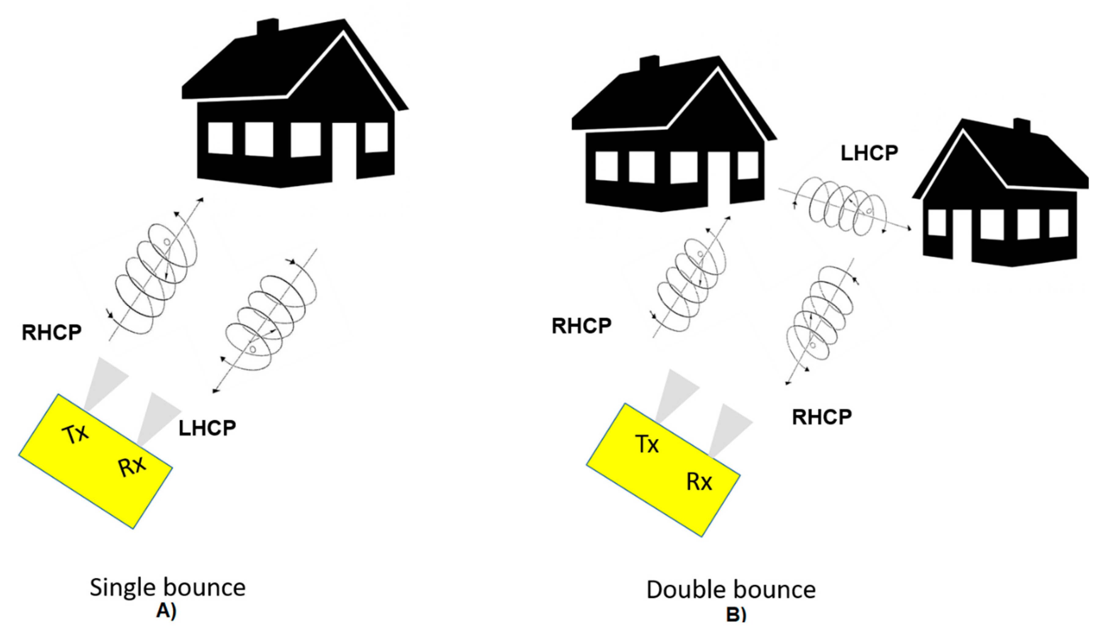
Anyway, circular polarization has been analyzed in a very few cases, and the interest to investigate the CP response of natural media, the topic of this paper, comes from the general features of this polarization, among which its ability to be less affected by the multipath effect is outstanding. It is well known that when the transmitted circular polarized wave is reflected from a surface, along a direction whose incidence angle is higher than the Brewster angle [21], it turns the handedness of the rotating electromagnetic field. In Figure 1, we resume the features that characterize the propagation of CP in the presence of symbolic targets.
After a bounce, the backscattered field propagates in the opposite direction with respect to the transmitted signal. The same rotation direction that would be described as “right-handed” circular polarization, RHCP, for the incident beam is “left-handed” circular polarization, LHCP, for propagation in the receiver direction, and vice versa. For this reason, in the case of a single bounce, a radar provided with the transmitting and receiving antennas with the opposite direction of rotation receives a strong signal. On the contrary, if the two antennas are co-polar, i.e., with the same direction of rotation, the detected signal is very low. When two bounces occur before reaching the receiving antenna, the situation is the opposite. In general, for an odd or even number of bounces, the situation is analogous; although due to the rapid decrease of the signal strength occurring after multiple bounces, the phenomenon is of minor concern. Therefore, by combining co-pol (RHCP and RHCP or LHCP and LHCP) and cross-pol (RHCP and LHCP or LHCP and RHCP) pairs of transmitting and receiving antennas, the contribution from even or odd bounds can be enhanced or minimized. Furthermore, using linear polarized antennas, the reflecting surface does not reflect the signal precisely in the same plane, therefore, the signal strength is weakened. Since circular polarized antennas send and receive in all planes, the signal strength suffers a minor decrease. In circularly-polarized systems, the reflected signal is returned in the opposite orientation, largely avoiding conflict with the propagating signal; the result is that circularly-polarized signals can better penetrate and bend around obstructions. Multi-path is caused when the primary signal and the reflected signal reach a receiver at nearly the same time; linear polarized antennas are more susceptible to multi-path due to the increased possibility of reflection.
Infrastructures and natural media often exhibit non-regular surfaces, and targets’ distribution, and multiple reflections frequently occur: CP measurements are theoretically expected to provide better performances in terms of phase stability and targets’ identification, due to the reduced multipath interferences which characterize this polarization configuration. Furthermore, in literature examples, the potential of CP measurements to detect targets with a specific shape can also be found, especially in studies based on planetary missions based on radar imaging sensors [22,23]. On the other hand, the main drawbacks of the CP system are: (i) A lower efficiency in antenna gain, (ii) a complex design especially when CP is requested in a large bandwidth, and, finally, (iii) a lower diffusion and availability.
This paper reports some experimental results obtained acquiring data through a terrestrial radar, using different combinations of linear and circular polarized antennas. The polarization diversity is evaluated with an empirical approach comparing and analyzing the different responses, looking for the main differences between circular and linear combinations. The study introduces the topic, showing some tests carried out with simple targets using a pair of patch antenna arrays designed to operate at the Ku band frequencies reserved for TRI/GB-SAR use. The two circular polarized patch arrays specifically designed and developed for this study [24] were mounted as transmitting and receiving antennas in a largely diffused GB-SAR commercial system, the Ibis-L manufactured by Ids. The antennas can be used, in principle, with any similar apparatus working in the same band, provided that the used radar sensor is capable to interface through standard connectors or waveguide flanges. The study tries to evaluate, on the basis of some experimental data, if the circular polarization response of natural media and artificial targets can improve the interpretation of the radar images, with respect to the standard co-polar VV configuration, commonly used in TRI. The goal is to investigate how different polarization combinations in terrestrial radar interferometry affect the coherence and amplitude dispersion of natural media, and in particular whether the circular polarization can improve the identification of stable scatters.
The paper is organized in five sections. After this general introduction, the instrumentation characteristics and the methods used to acquire the radar response with different polarizations are described. The following section describes the results of some experimental tests designed to estimate the polarimetric features of single targets and a heterogeneous scenario, including an urban area surrounded by vegetation. First, simple tests using the radar sensor in a real aperture radar (RAR) mode are carried out to assess the capability of the system to provide a sufficient polarization purity. Then, the results of a two-days experimental campaign, carried out in an area including a small village affected by a large landslide, and monitored using the radar in the GB SAR mode, are presented and commented on. Different combinations of receiving and transmitting antennas are used to evaluate the behaviour of some parameters of main concern to individuate coherent areas in radar interferometry. A discussion section is then dedicated to the main outcomes of the study. A conclusions section is dedicated to a summary of the paper content, and suggestions for planning further experiments.
2. Materials and Methods
In this section, the measuring system and the novel antennas used to carry out the experimental campaigns are introduced, with a more detailed description dedicated to the antennas, which represent the novel aspect of the proposed approach. The basic rationale of this study consists in first evaluating the polarimetric performances of the new acquisition system, using circular polarized antennas in a real aperture radar (RAR) configuration to measure the response of simple basic targets. Furthermore, the same radar transceiver is used to acquire, by means of a standard linear GB synthetic aperture configuration, images of a natural scenario, with different polarization combinations.
2.1. The Radar Setup
This study is based on the use of an apparatus, the Ibis-S [25], which in the commercial version, is not provided by multipolarization equipment, acquiring only the co-polar vertical polarization. The design of the radar with polarimetric capabilities, performing simultaneous acquisitions of the different polarization signals, demands an increased complexity of the system: At least two different receiving sections, with different antennas guaranteeing an adequate purity in their polarization response, are necessary. In addition, this approach requires complex calibration procedures, which jointly involves the transceiver and the antennas: See, for example, [17]. When the simultaneity of the acquisitions is not necessary, because the polarization properties of the observed media are supposed to be stable or slow and varying with time, a single transceiver section can be adequate. In this case, acquisitions with different polarizations can be obtained by simply substituting the antennas in subsequent acquisitions, and only the mutual antenna performances determine the polarization purity of the measurement. On this basis, for this study, two original antennas operating as CP were developed for remote sensing (RS) applications based on ground-based microwave interferometers, in both RAR [26] or SAR configurations [1,2], as an alternative to the standard linear polarized antenna.
2.2. The Circular Polarization Antennas
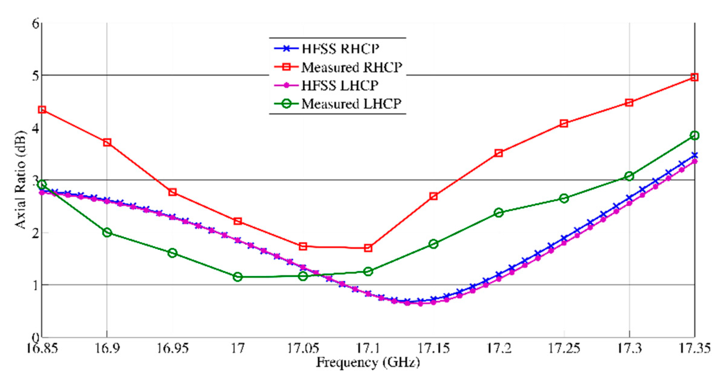
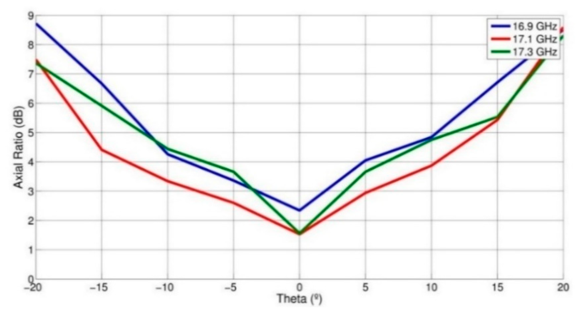
In this study, two type of antennas are used. The acquisition of linear polarized (LP) data is carried out using two pyramidal horn antennas provided by the producer of the apparatus, both with an approximated value of 20 dBi gain. This type of antenna is usually used for its regular phase response, high isolation between orthogonal fields (V/H linear), and high gain. Despite these qualities, with respect to a patch array, plane, and light, this aperture antenna is bulky and heavy. To arrange a multipolarization system able to acquire cross-and co-CP responses, two patch antennas were implemented, respectively, for LHCP and RHCP. As printed antennas, they offer the possibility of low cost, low weight, and scalability to a high gain version compared to conventional horn antennas; this latter condition results in the selection of microstrip technology. The requirements of this antenna array to be used in a terrestrial radar are: (i) An operating band of 17.05 ± 0.15 GHZ [27], (ii) sufficient polarization purity in this band, and, finally, (iii) the capability to be mounted into the available radar apparatus. The design of the array is based on the combination of four linear polarization elements to be produced, with an appropriate sequential rotation of the elements and the feeding network, RHCP and LHCP [24]. The parameter which allows the evaluation of the degree of circularity of a polarized antenna, which is important to assure in this study as a reliable comparison between the different responses of a target when observed through LP or CP observations, is the axial ratio, AR, [28]. AR is 0dB when the antenna provides a perfect circular polarization; in fact, it varies with the frequency and the direction of the antenna pattern [28]. In the operating band of the Ibis-S transceiver used in this study, from 16.9 GHz to 17.2 GHz, the AR was calculated during the design of the array, carried out using HFSS software [29], and it was also measured in an anechoic chamber. Results of the antenna tests are reported in Figure 2, which shows the comparison between simulated and measured AR as a function of the frequency, and Figure 3, showing the simulated AR as a function the viewing angle theta with respect to the antenna axis for three frequency values spanning the entire operating bandwidth. Observing these results, and considering that 3 dB is usually considered a satisfactory value, the results of the measurements and of the simulation assess a sufficient degree of circular polarization for the implemented patch arrays.
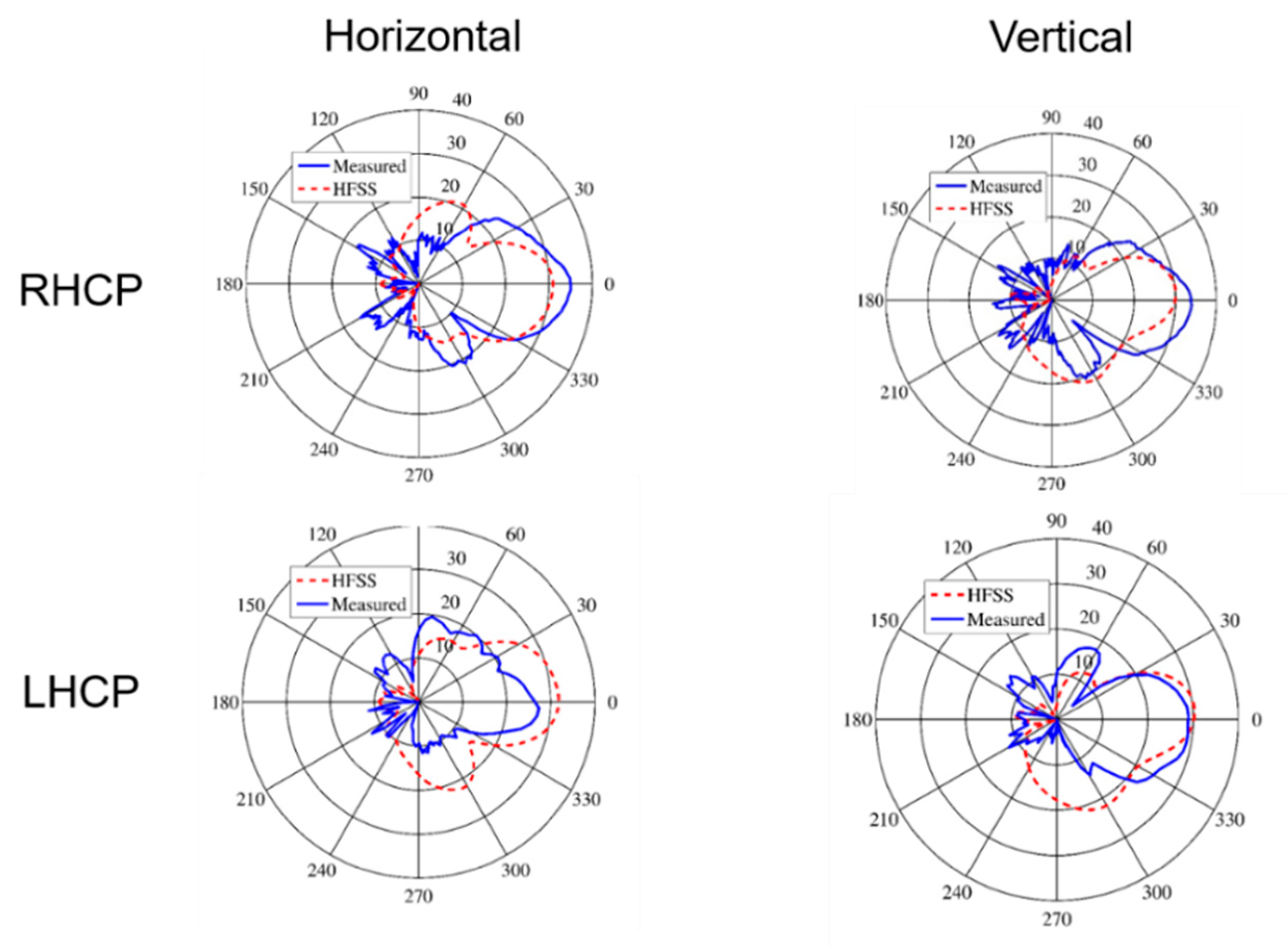
To characterize the two patch array antenna, the radiation pattern, for the horizontal and vertical plane were first simulated, and then measured in an anechoic chamber: Figure 4 shows the results.
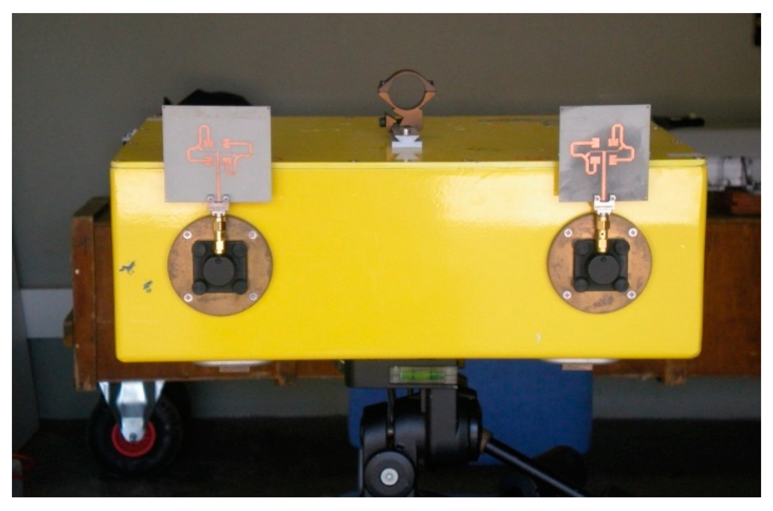
The two antenna array prototypes were designed, produced, and tested at CTTC. In Figure 5, a photo of the two prototypes mounted on the Ibis transceiver is shown; it is of note that the two patch arrays are connected through a waveguide-SMA connector adapter, which can worsen the matching between antennas and the transceiver, but which is necessary to interface the antennas to the Ibis transceiver. The microstrip circuits used to obtain the RHCP and LHCP patch are specular with respect to the feed line direction (see Figure 5).
When comparing the data acquired with the two different configurations, it must be considered that, with respect to the LP horn antennas, the patch antennas developed for LHCP and RHCP are worse performing in terms of gain directivity, antenna efficiency, and isolation between the receiving and transmitting elements, all factors which affect the amplitude response. This inconvenience is partially due to the design choice, i.e., a limited size of the patch, and to the higher mismatch expected for fitting the patch antenna and the waveguide connection of the sensor (see Figure 5).
As measurements of the patch antenna gain in an anechoic chamber were not available, we decided to estimate the CP antenna gain in a free space environment, using a less rigorous approach, described in the next Section 2.3. Although these estimates can be affected by errors due to multipath, we used these results in our analysis on the basis of the following rationales: (i) The measurements were carried out with the targets in a largely fulfilled far field condition, where the free space condition is similar to an anechoic chamber response; (ii) our main goal was not to evaluate the absolute gain of the CP arrays, but their relative values with respect to those of the standard horn provided by the transceiver manufacturer: A high accuracy is not mandatory. The objective was to compare the performances of the different transceiver-antenna setup; (iii) all the data used to compare the gain from the two different polarization configurations were obtained in the same environment, where multipath is negligible. In addition, radiation measurements were operated in a far field condition. For this reason, as far as the different radar acquisitions are concerned, to compare the acquired data, we first provided an estimate of the new antennas’ gain when mounted on the transceiver.
2.3. Circularly Polarized Antennas’ Gain Estimate
To compare the amplitude responses from measurements carried out with different antennas’ combinations, we needed to estimate the gain of the two CP antennas when mounted on the transceiver.
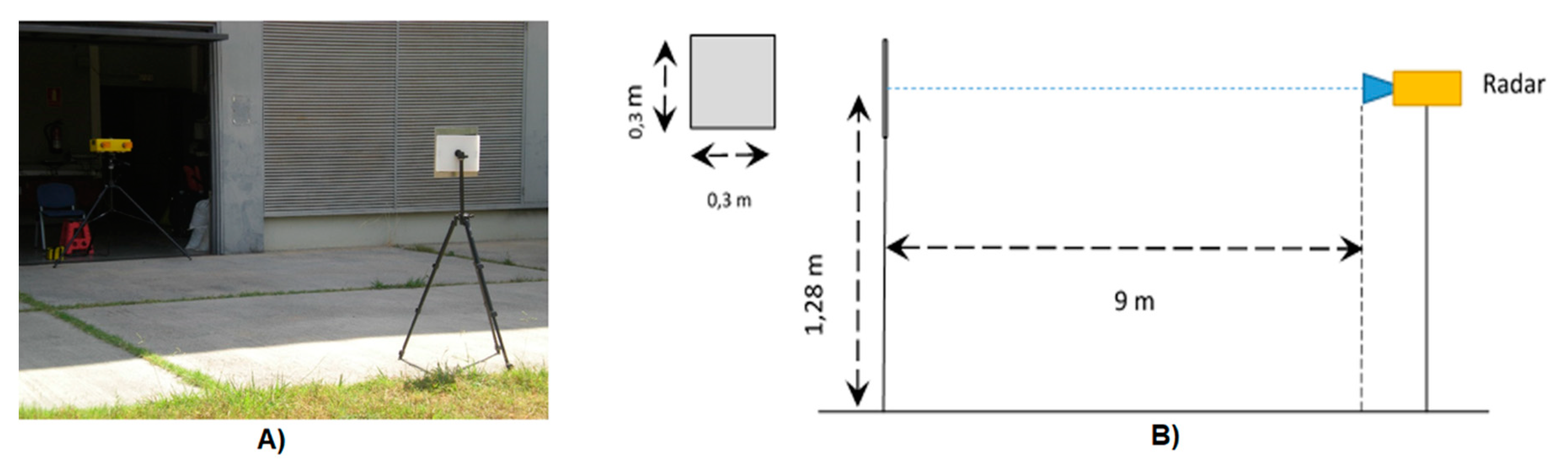
The apparatus is placed in a fixed position in front of a reference target: An aluminum square plate, size of 30 cm, located at 9 m from the antennas, a distance complying with the antennas’ far field condition, with an estimated radar cross-section (RCS) at a perpendicular incidence of 25.3 dBsm; in this first test, in the RAR configuration, targets are ranged with a 0.5 m resolution. Using the gain comparison technique [28], considering the LP horn (20 dBi) as a reference, assuming that at first approximation the two CP patch arrays get the same value, we can execute a simple procedure based on two measurements. In Figure 6, a scheme of the setup and a picture is shown. In the first acquisition, the transmitting and receiving antennas are a VV horn and CP patch array, respectively; in the second acquisition, two patch arrays in a cross-polar configuration are used: RHCP and LHCP. In Table 2, the values of the received power, estimated through the peaks identified in correspondence to the target location, with respect to the thermal noise of the receiver [25], are reported. To calculate the gain of the patch, after applying a simplified form of the radar equation [30], the following expressions for the received power, Prec, were obtained:
where:
- : Received power at measurement .
- : Transmitted power (at the port of the transmitting antenna).
- : Gain of the linear polarized horn.
- : Gain of the circularly polarized patch array.
- : radar cross section of the target.
- : propagation and loss factor.
Combining Equations (1) and (2):
The 3 dB term in Equation (1) is added to compensate the comparison of the gain between a linear polarized and a circular polarized antenna [28]. The value of 7 dBi, which includes possible loss mismatching, is in agreement with the value expected from the simulation.
Using this value, we can compare the backscattering response of different polarization configurations for any targets, and hence better understand their polarimetric features.
3. Experimental Results
This study is based on the acquisition of experimental data, collected to evaluate whether coherence and amplitude dispersion of backscattering responses from natural media have different behaviours when observed through circular polarization antennas, potentially improving the identification of stable scatters. To this aim, two experimental campaigns were carried out: The first dedicated to measure the co-polar and cross-polar response of elementary targets, namely a concrete wall and a light pole, in the RAR mode. Then, images of a small urban area acquired in the SAR mode, and using different combinations of polarization, and during two different temporal time intervals, were analyzed.
3.1. RAR Acquisitions: The Response of a Wall
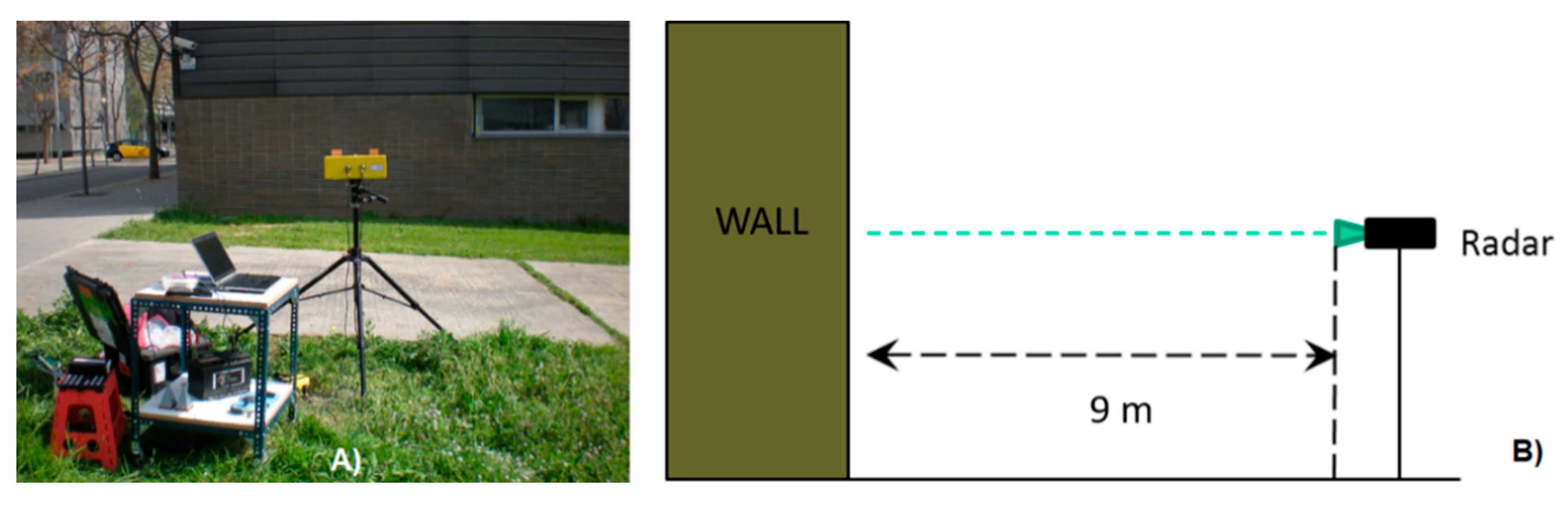
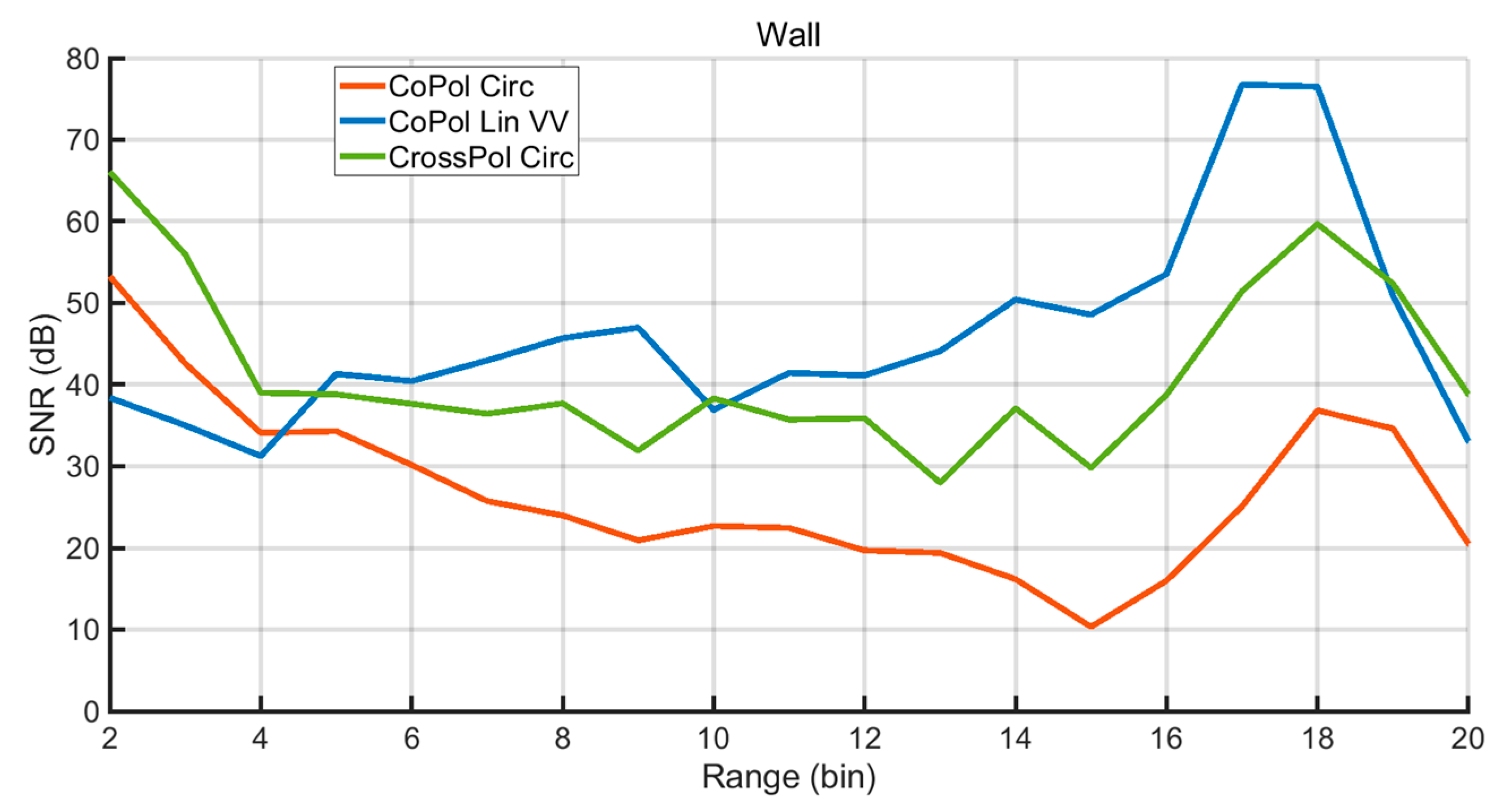
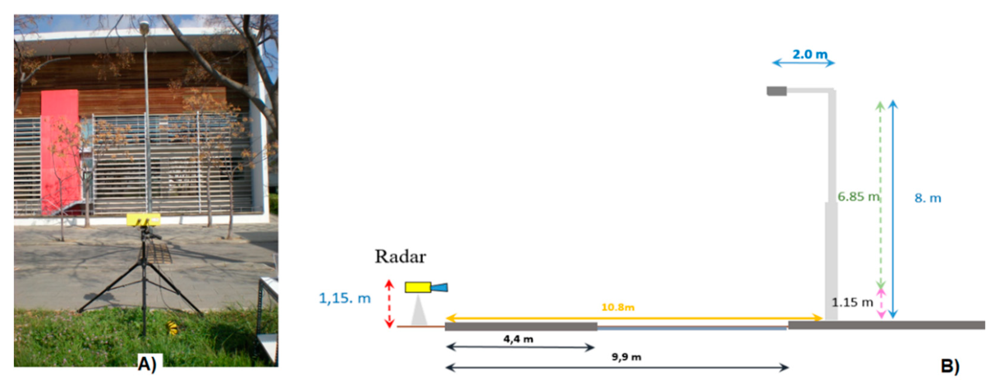
To evaluate the actual capability of the system to separate the two polarization configurations, a radar acquisition was carried out in front of a wall. Figure 7 shows a picture of the set up. In Table 3, the values of the received power for three different combinations are shown: Co-polar VV LP linear, Cross-polar CP Circular, and co-polar CP. We did not acquire this combination focusing on the cross pol and co-pol difference. Considering the geometric and dielectric characteristics of the target, we did not expect significant differences to change the polarization rotation verse. In Figure 8, the corresponding range profiles are plotted, where the wall surface is identified in bin 17–18. This slight difference between the LP and the CP measurements can be due to the delay introduced by the patch array match. As expected, the highest amplitude of the reflected signal is for the VV configuration, while the weakest response is the circular co-polar CP.
Considering that the target is a dielectric surface, perpendicular to the radar line of sight (LOS), and which completely fills the antenna’s field of view (FOV), the measurements can be used to estimate the difference between the cross and co-polar CP response. In this case, where a single bounce is expected, the estimated value is 23 dB. It is of note that the difference between VV and cross-polar CP, measurement 1 and 2, is attributable to the difference of gain.
3.2. RAR Acquisitions: The Response of a Lightpole
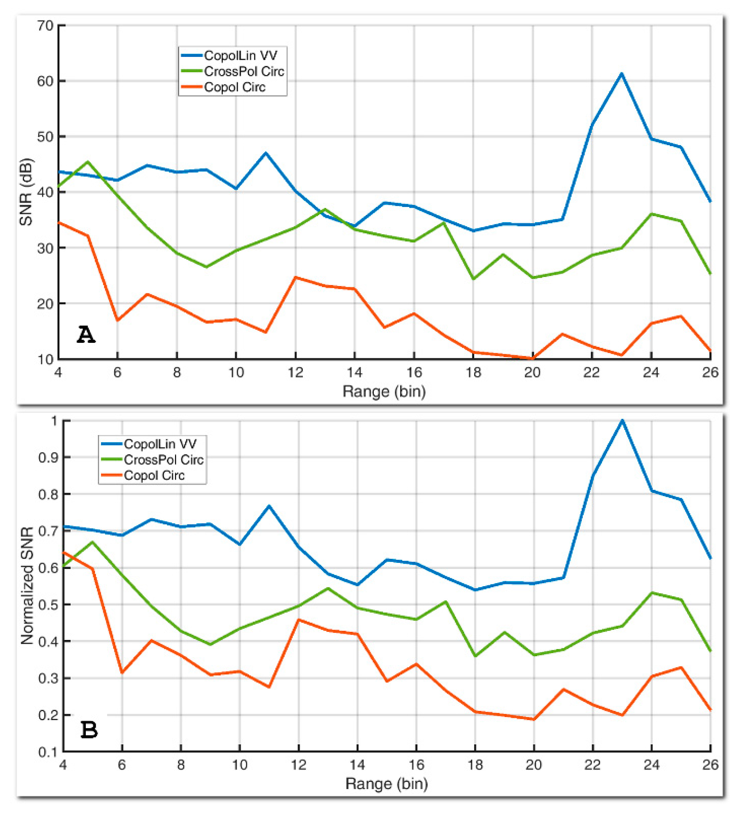
A further test to analyze the different responses between LP and CP antennas was carried out, acquiring data in front of a lightpole. In Figure 9, the geometry of the acquisition and a picture of the setup are shown. Observing the signal-to-noise ratio (SNR) profile in Figure 10A, VV obtains, as expected, the highest intensity, while RR is the lowest.
In Figure 10B, the relative values of measured intensity, normalized to the maximum, are also shown to check the influence of the different gain of the antennas on data interpretation. The presence of a single bounce and the vertical structure, like a cylinder, gives a strong reflection of VV polarization. In the SNR profile, we observe that the cross-polar CP signal is much higher (>20 dB), than the co-polar CP. Observing the scheme of Figure 10B, some reflections (minor peaks) are present previous to the light pole, which are associable to the discontinuities in the asphalt. The data analyzed confirm that the measuring apparatus has a sufficient polarimetric capability that is able to enhance the features of the two CP configurations.
3.3. GBSAR Acquisitions of a Landslide Area
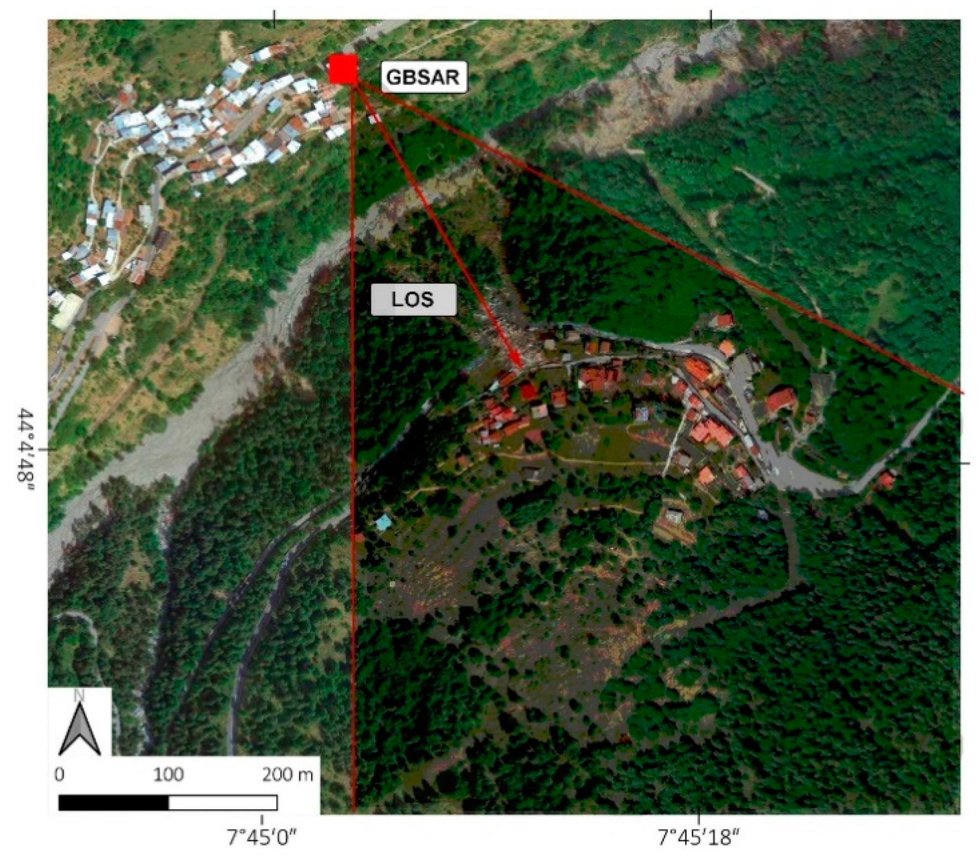
In this section, the data used to analyze the response of different polarization combinations were obtained during a two day long GB SAR image acquisition. The scenario is heterogeneous, consisting of a small urban area, including buildings, and debris due to a landslide; all is surrounded by a vegetated area. Figure 11 shows the orthophoto of the area monitored through the GBSAR. In the centre of the picture the collapsed are is clearly distinguishable, composed of very heterogeneous material: E.g., bricks, rocks, roof pieces, undulated metal plates, soil. The radar data used in this study were acquired during a monitoring campaign organized within a H2020 project (HEIMDALL Project Number 740689 [31]). The site is a small village located in Northern Italy, at 1300 m asl, namely Monesi di Mendatica, where a large landslide occurred in November 2016, destroying a main road and several buildings, and causing the evacuation of all the inhabitants. The GB-SAR was installed in 2017, in a site in front of the area affected by the landslide, placed at approximately 300 m from the scene, and at the same altitude; therefore, the elevation angle of the radar antennas is zero.
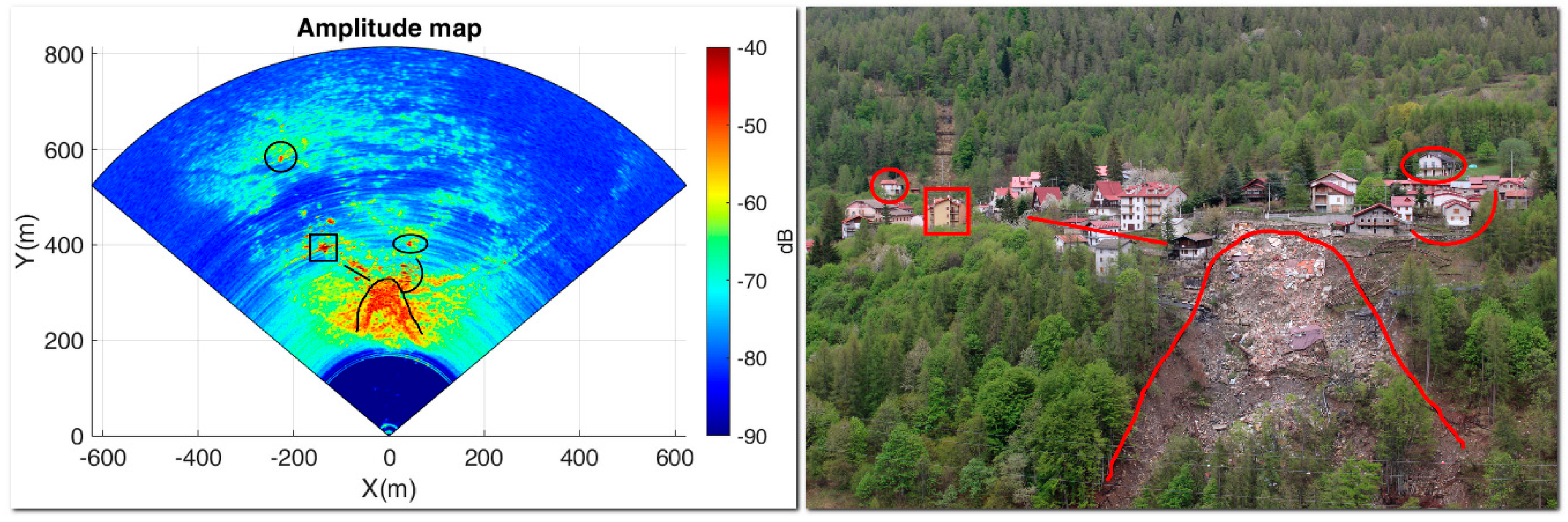
Figure 12A,B show an amplitude image (VV pol) in radar coordinates, and a photo of the main area of the landslide, respectively.
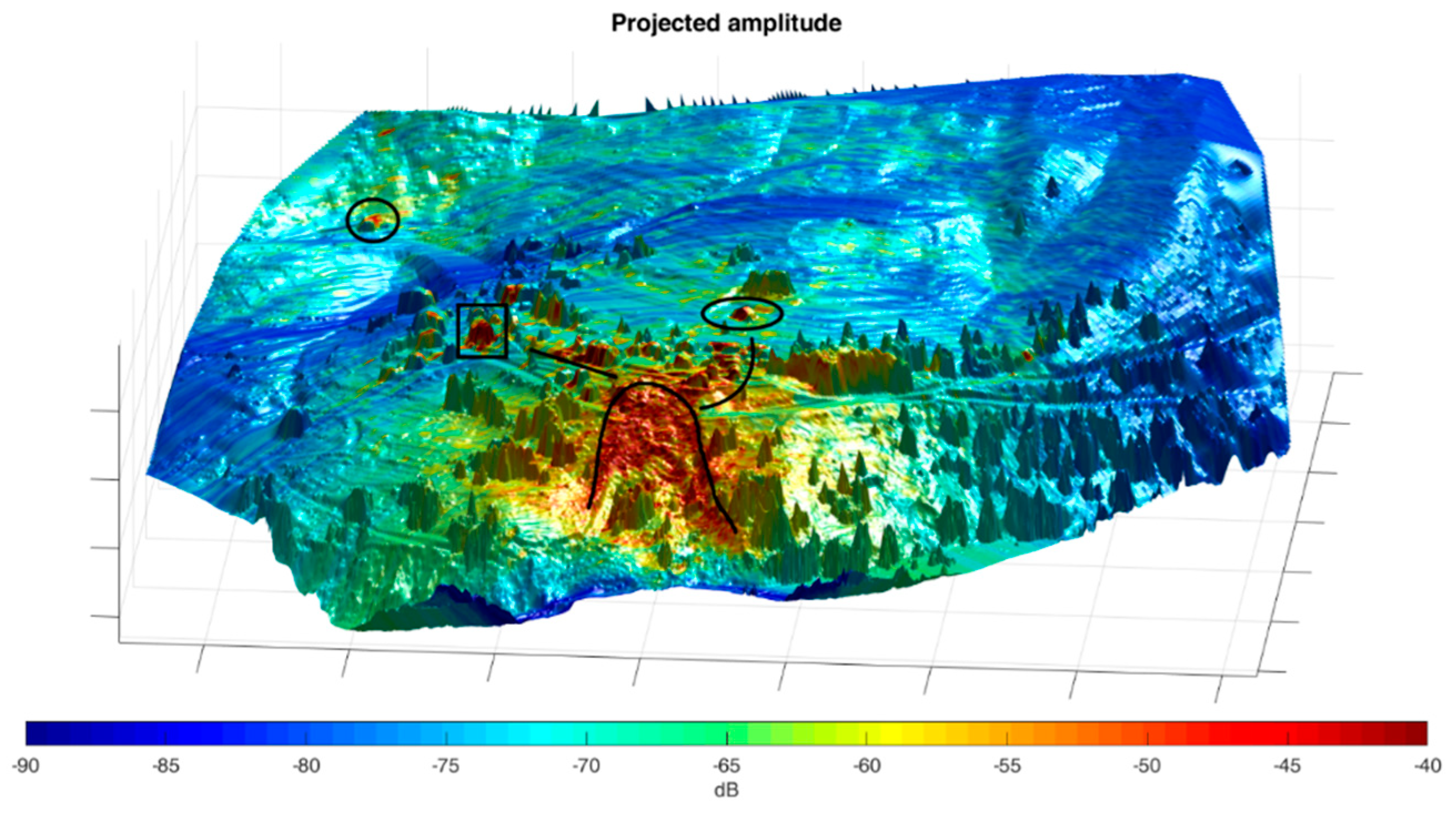
Some targets are marked to make it easier to recognize the correspondence between the radar map and the real scene. Figure 13 shows the same radar data of Figure 12A projected on the digital surface model (DSM) to support the data interpretation.
The data were analyzed by comparing the polarization differences considering two temporal scales: A short one, where several combinations were observed, and a long one, focused on the linear vertical co-polar and the circular crosspolar cases. The first case corresponds to a temporal interval of approximately 3 h (i.e., 20 images), while the second one covers a 24 h lapse (i.e., 200 images).
In the following section, we focus on the radar response considering two parameters: The temporal dispersion of amplitude (DA) and the coherence (COH), which are the main parameters related to the statistical reliability of interferometric processing. High values of coherence and/or low values of DA are quality indexes related to the accuracy of the retrieved interferometric parameters. DA is defined by Equation (5):
where are the temporal mean and standard deviation of the amplitude of the analyzed pixel, respectively.
3.3.1. The Short Time Series
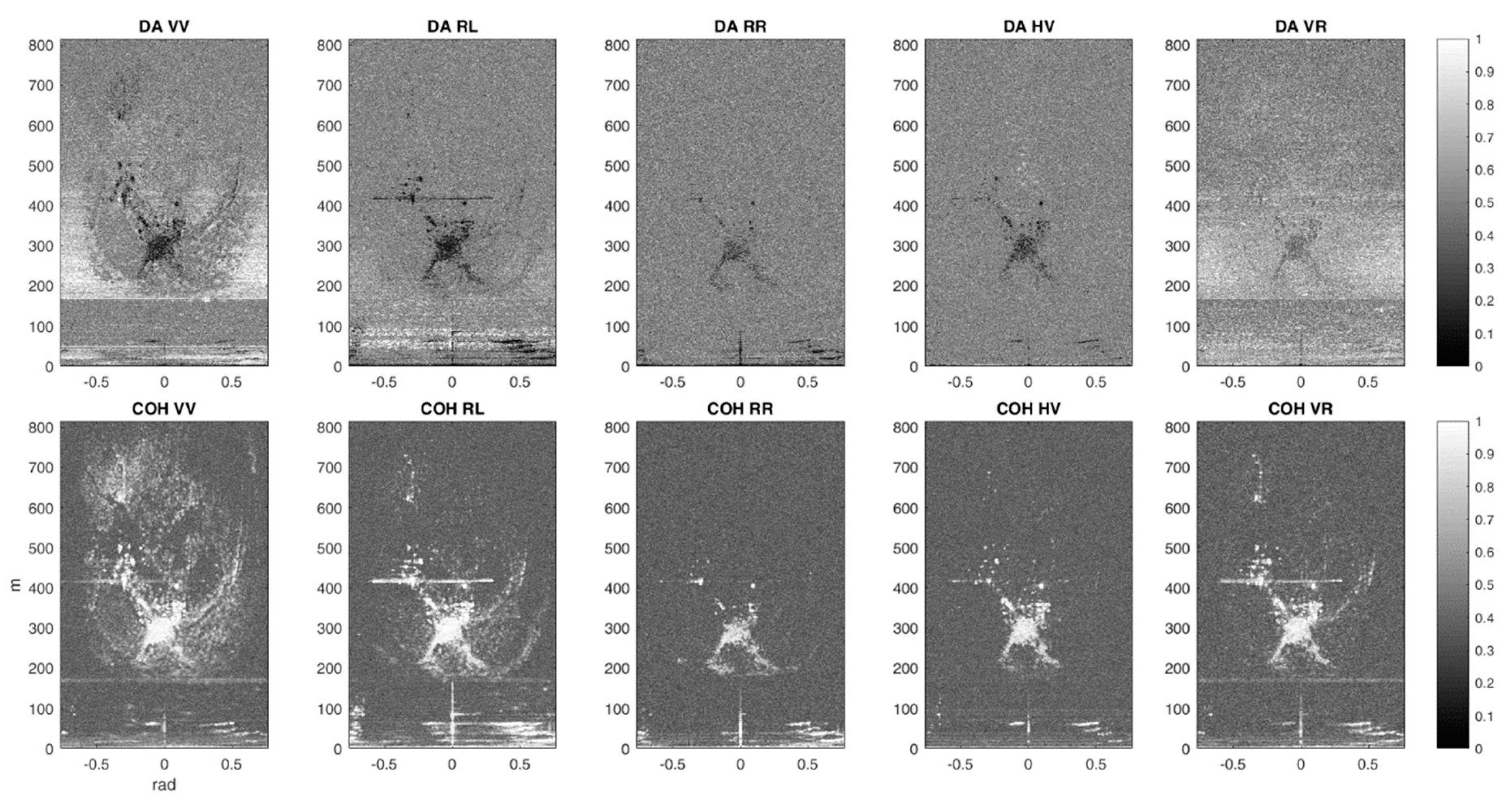
The set of images below were acquired during two hours (20 images) for each configuration. Figure 14 shows the DA and the COH of the five cases shown in Table 4. From these plots, we observe the following main remarks. VV shows the lowest DA on buildings, as expected, but also vegetation is low, due to the short temporal lapse analyzed: Indeed, coherence also maintains very high values. In this specific case, it is difficult to identify the differences among different targets, due to the short time lapse. The cross-polar HV shows high coherencevalues on buildings, but very low values on vegetation.
The very high and noisy DA reduces its utility when interferometric techniques are applied. RL shows a low DA and high coherence on buildings. As for VV, considering that the coherence on the vegetation is low, RL can be used both for selecting interferometric scatters and for classification purposes. The RR configuration shows good coherence on buildings, and some specific targets where even bounces are present, but vegetation backscattering is very low, comparable with the noise of the areas where no radar targets are present. Furthermore, RR presents a high amplitude variability.
Finally, for the “hybrid configuration”, VR, i.e., transmitting in linear vertical configuration and receiving in RHCP, one can observe a coherence similar to that of RL, but it has the highest DA. This result is not peculiar considering that this combination can be considered at the same time as being partially co-polar (VV) and cross-polar (VH). Observing these results, the two configurations which show a good range in DA and COH are VV and RL; for this reason, we dedicated the second part of the data acquisitions, lasting a longer temporal interval, only to these two combinations (see Section 3.3.2).
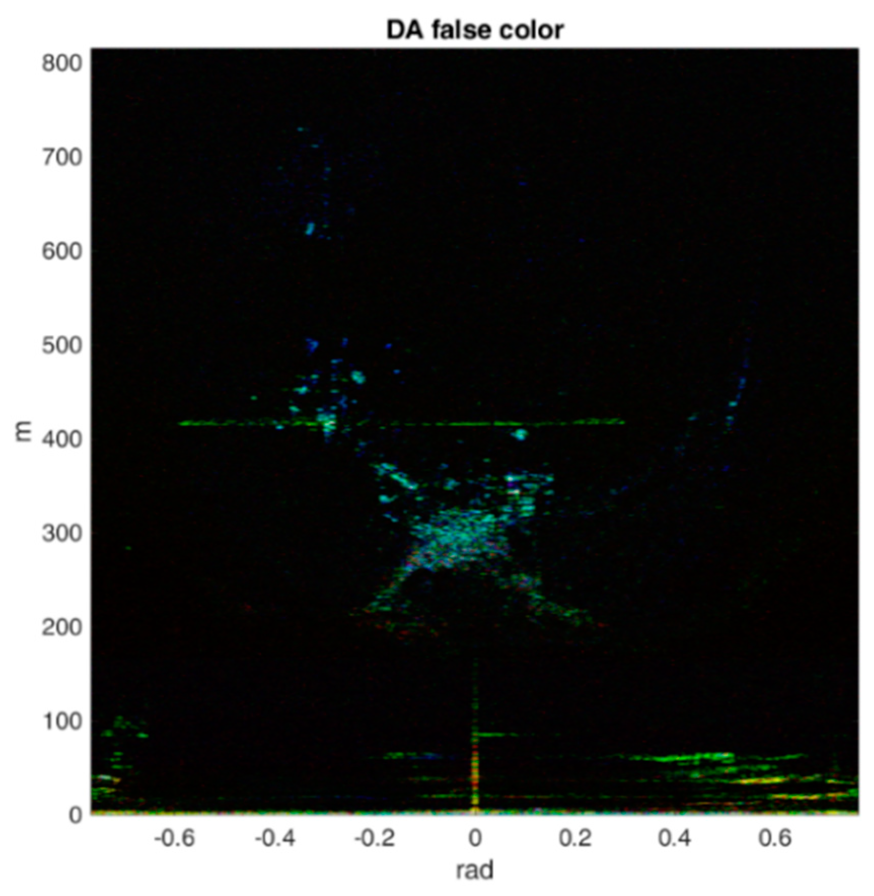
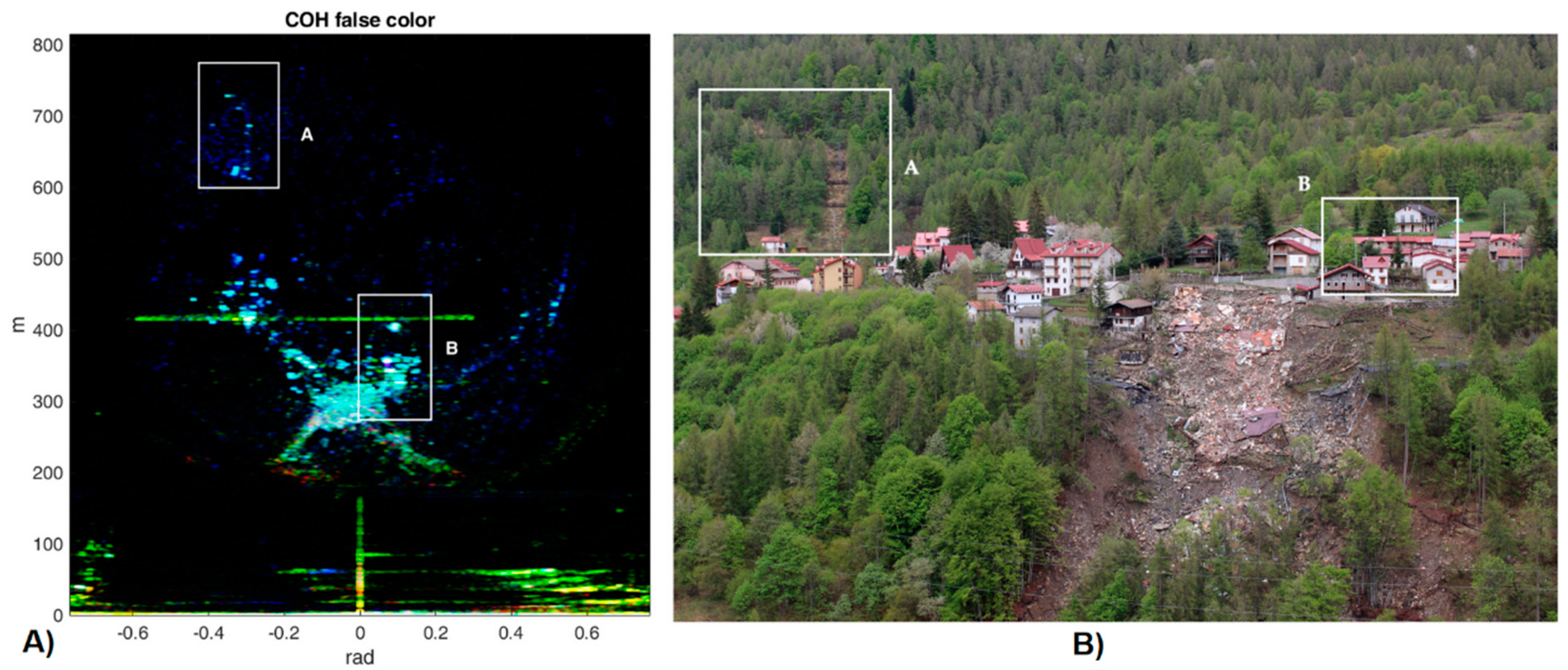
An attempt to benefit from these comments is to try a simple classification among elementary classes, such as buildings, vegetation, and incoherent material in the middle of the landslide area. To this aim, we composed images in false colours combining in a RGB image, the DA and COH of three different polarization configurations. Therefore, we associated to the channels red, green, and blue the polarizations of RR, RL, and VV, respectively. From the false color-DA map (Figure 15), no clear indications arise, while the false color-COH, plotted in Figure 16A, deserves some comments. Cyan colour reveals that RL and VV have almost the same behaviour. Vegetation is represented by dark blue due to relatively low COH. The map demonstrates from a qualitative point of view a certain capability to separate building from vegetation areas using this combination of the three polarizations.
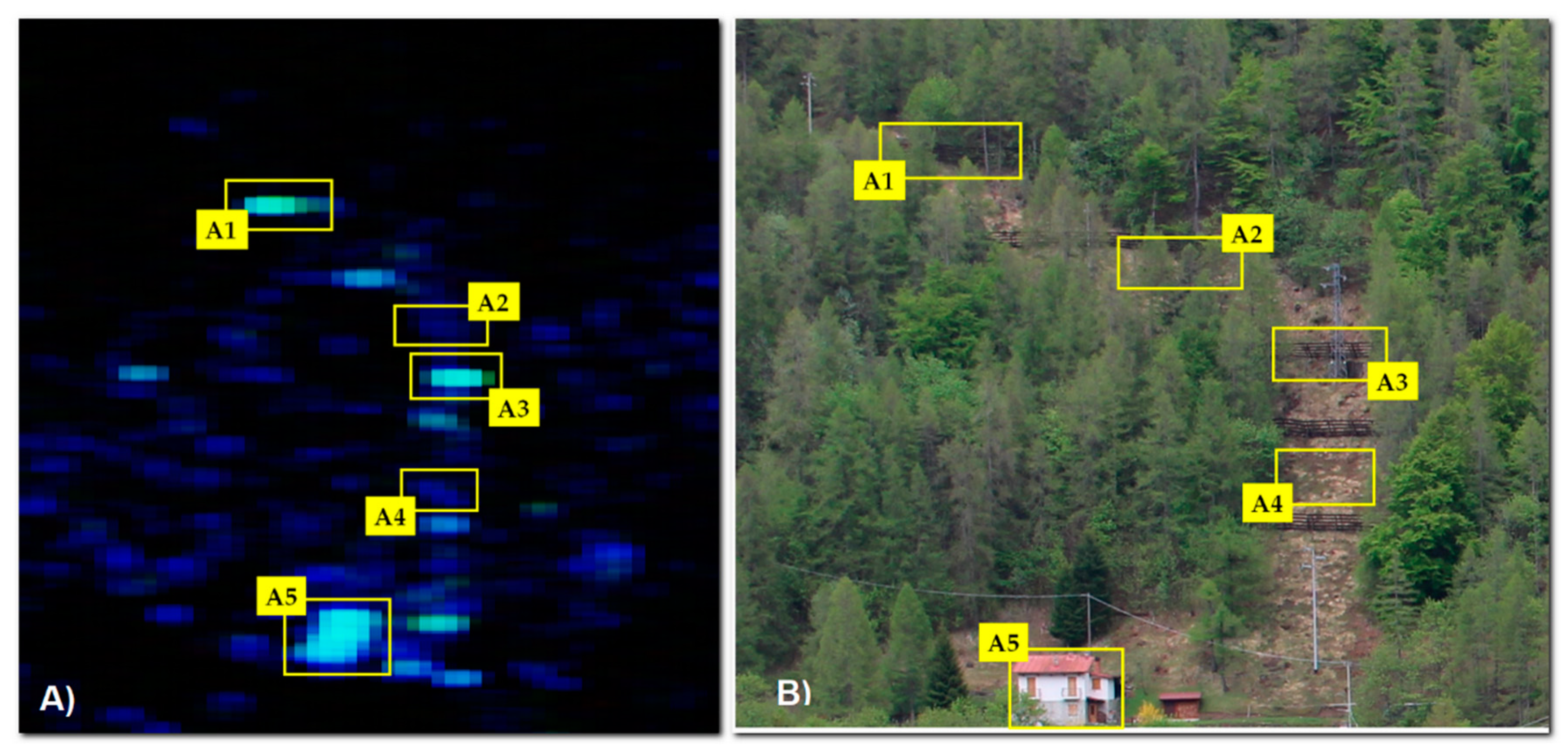
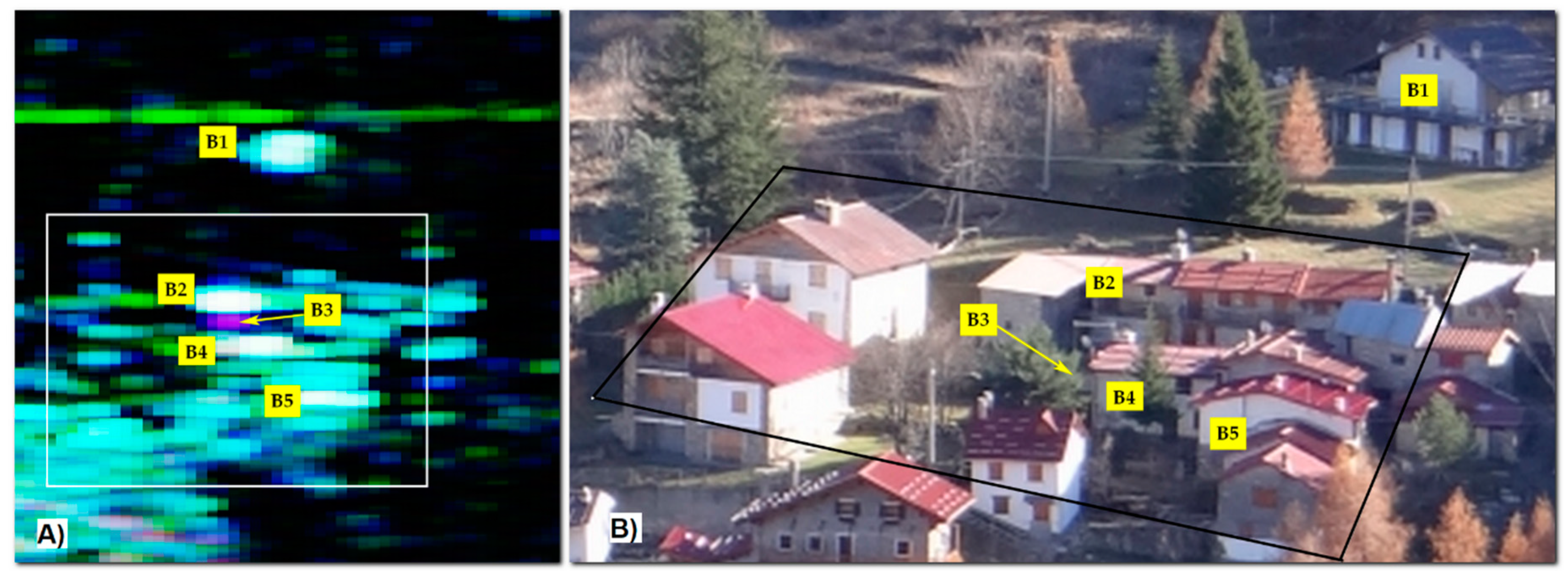
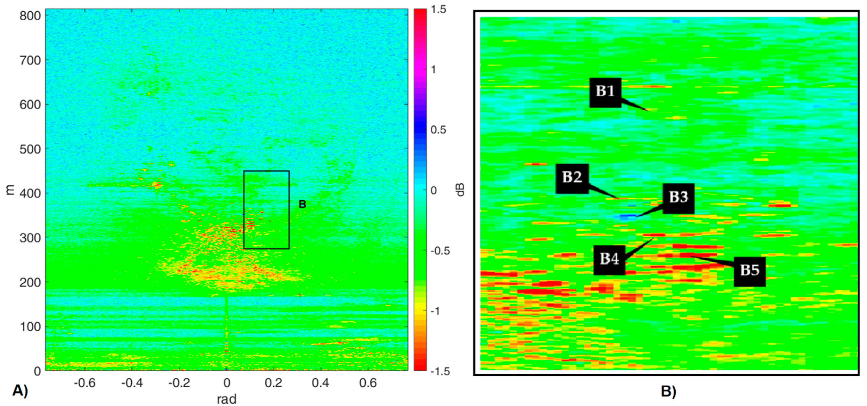
A more detailed analysis on the coherence behaviour was carried out for two specific areas, which are marked in Figure 16A, and detailed in the pictures of Figure 17B and Figure 18B. The two areas correspond to some fences and vegetated areas (A) and a group of buildings (B), respectively.
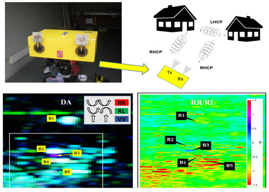
The VV and RL coherence values are almost equivalent on fences and buildings, but VV is much higher than RL and RR on vegetation. RR is generally low everywhere due to the prevalence of a single bounce response. In the area B, the response is different. Observing Figure 18A, where the targets are more visible, we note that for B1, B2, and B4, the backscattering amplitude is high for all the polarizations due to multiple bounces. For target B3, probably due to even bounces, the circular cross-polarization is low. A low value is obtained for the circular co-polarization due to a single bounce in B5.
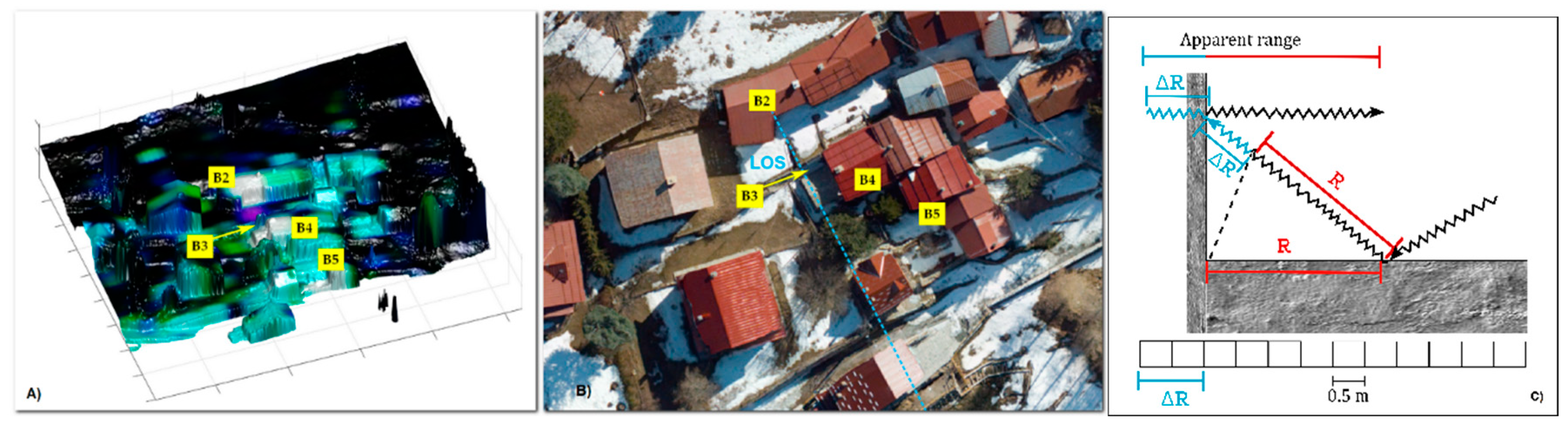
In Table 5, the single channel values are reported. Figure 19 shows the buildings from an aerial view and projected on the DSM. This picture allows for better interpretation of the response. For B2 and B4, the received signal comes from a multiple bounce, as confirmed by the high value for all the polarization. Target B3 differentiates from the others with a high RR, probably due to a wall-floor double bounce. In Figure 19C, a simplified scheme of the two scattering modes occurring in the small area is shown.
The relative phase between RR and RL was also calculated and analyzed. Nevertheless, we could not find any relevant behaviour, probably because the site is strongly affected by atmospheric effects that disturb the signal and that cause phase wrapping. Finally, in Figure 20, we show the RR/RL amplitude ratio. As expected, the amplitude of the void areas is almost equal, while the amplitude of vegetation is slightly higher for RL. More interesting is the analysis of this variable on the buildings, as shown in Figure 20B. In this case, the RL amplitude is much higher than RR, as already discussed in the previous sections, and it allows identification of the artificial targets, where the RL amplitude is stronger. Nevertheless, the ratio is not homogeneous on all the structures; its analysis reveals where the even/odd bounce modes prevail. In particular, Figure 20B shows that the targets, B4 and B5, reflect mostly in the single bounce mode, while in B1 and B2, the double bounce has a relevant component. On the contrary, B3 reveals that the RR amplitude is stronger than RL because a double bounce process occurs. Observing Figure 19A,B, one can note that the position of B3 corresponds to a flat area just a few meters behind a vertical concrete wall that forms a 90° dihedral where the double bounce occurs. The apparent farther position of the target can be ascribed to the path covered between the two bounces that is summed to the range between the radar and the concrete wall (i.e., the position of the first bounce).
3.3.2. The Long Time Series
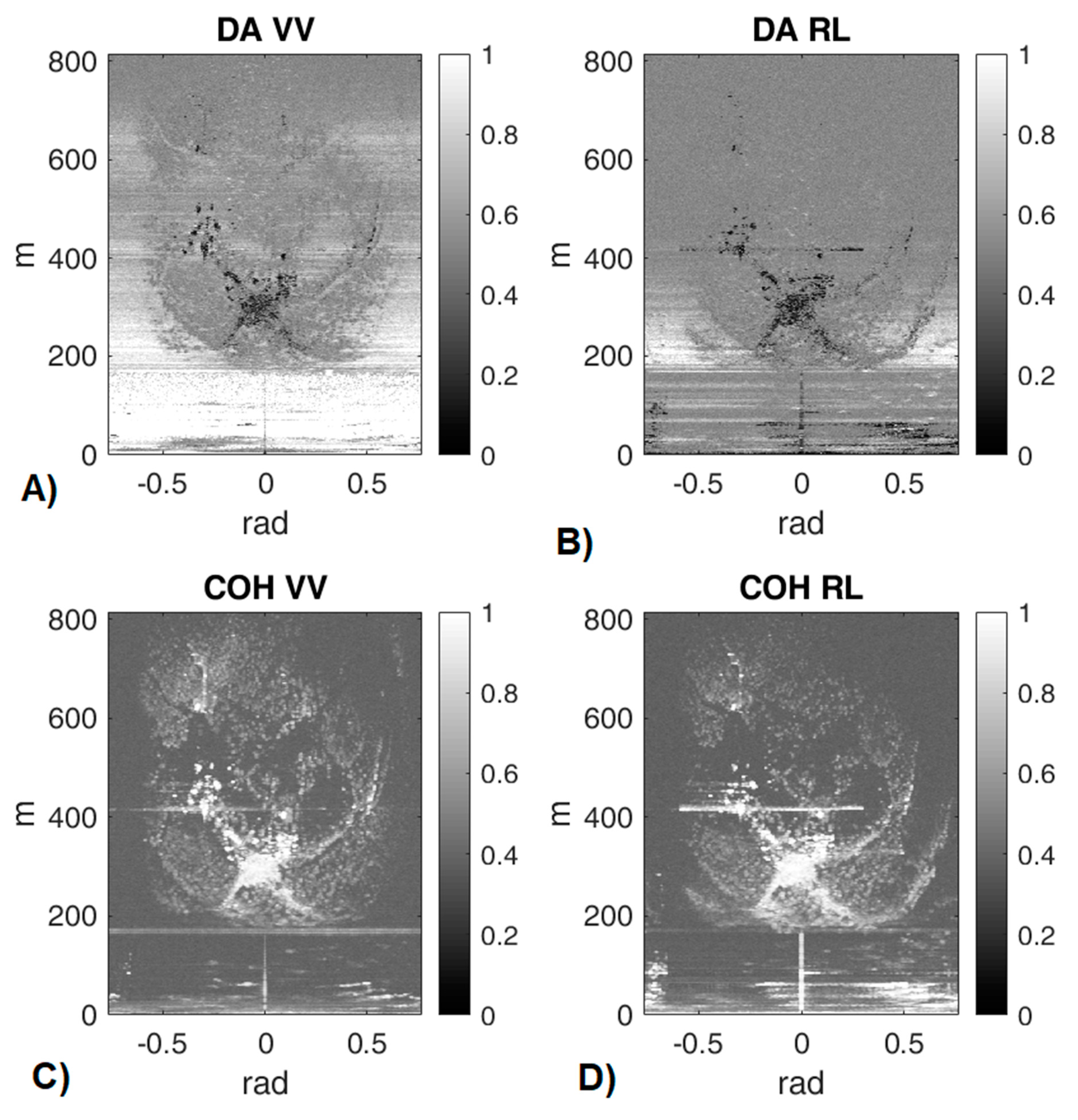
In this section, the results of two configurations, namely VV and RL, for a day-long temporal interval, are discussed, as shown in Table 6. In Figure 21, DA and COH are shown.
In general, DA VV is very high in the first 300 m, but this can be ascribed to the absence of targets and hence only represents the noise of the system. On the other hand, on the targets, it maintains a lower DA. DA of RL is quite uniform and assumes values similar to the areas subjected by relevant decorrelation in void areas, such as wood or grass. COH RL is high on trees despite the large temporal interval for the long series, and improves with respect to short measurements.
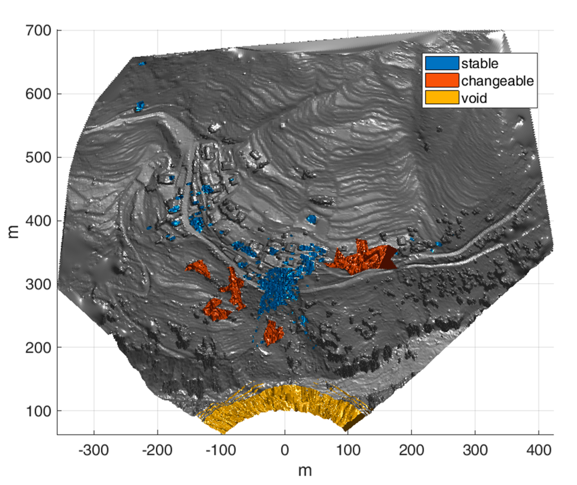
In this case, three areas were defined to further detail the analysis, as shown in Figure 22, where the DA is depicted on the DSM, with different colours for stable scatters (buildings), changeable scatters (mostly trees), and no signal (void).
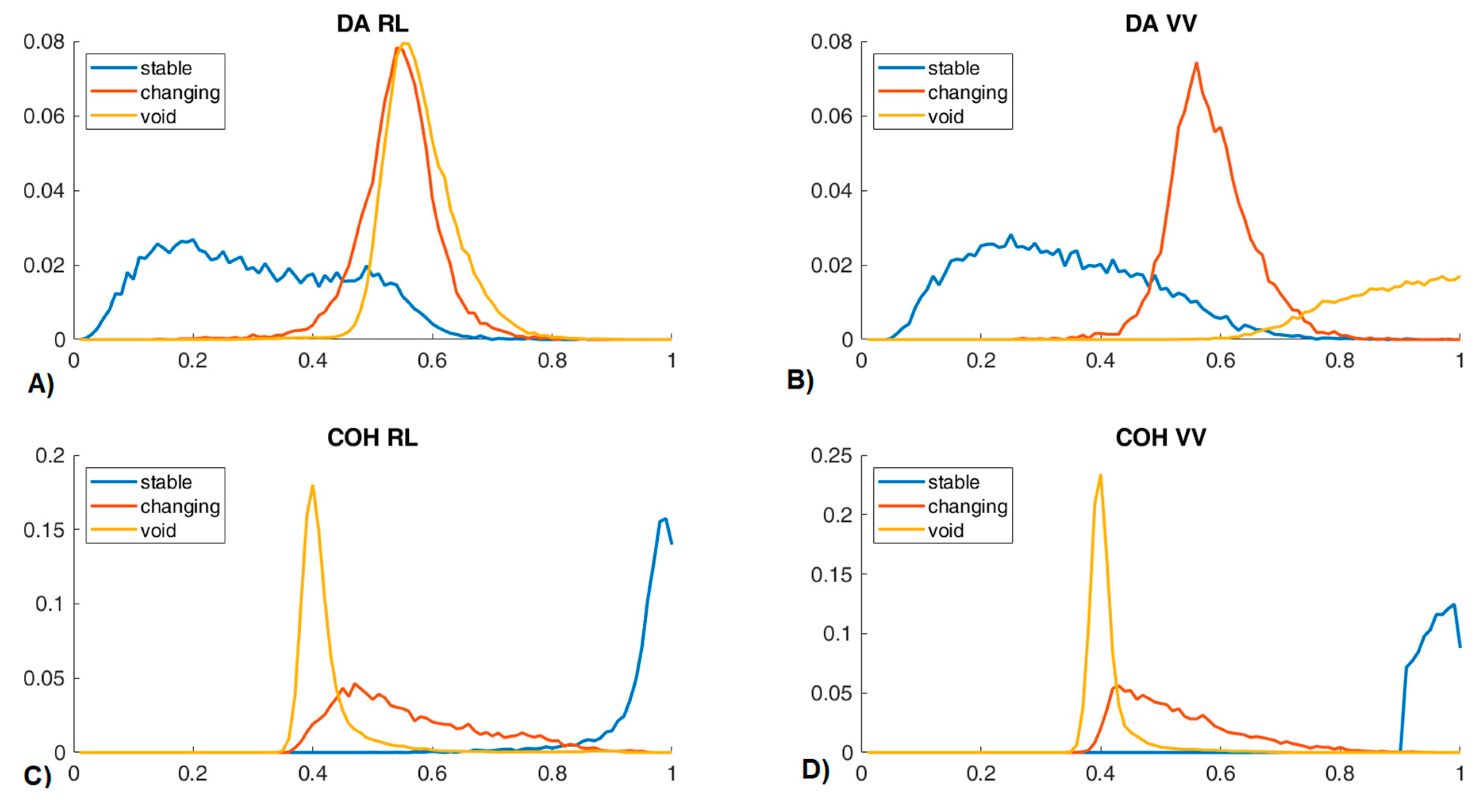
Calculating the probability density function (PDF) of the three ensembles, shown in Figure 23, the following comments can be made, which confirm the previous observations. For RL, the stable targets maintain low values of DA and high of COH, but only COH allows any distinguishing between no signal and vegetated areas: The DA of RL cannot improve the knowledge about these kind of scenarios. On the other hand, for DA in VV and RL, different behaviors are evident for the three sets (see Figure 23A,B).
The statistical analysis of these parameters of terrestrial radar interferometry represents a further characterization of the various polarization configurations and it highlights/suggests possible applications. For example, the proposed classes can be adapted to the scenario, and in the case of an alpine glacier, they can distinguish glacier surface and rocks, which is very important for atmospheric phase screen (APS) correction and for understanding purposes. Therefore, as expected, the analysis of the DA in VV configuration allows classification of different targets [32].
4. Discussion of the Results
Based on the experimental data analyzed in the previous section, we can assess and discuss the following outcomes. First, the radar system arranged with the novel antennas, despite the lack of a rigorous polarimetric calibration, was demonstrated to be appropriate to provide a polarization capability to distinguish single and multiple bounce responses from reference targets. Although fully polarimetric high performing systems have been used by other researchers to investigate the response of natural surfaces ([15,16,17,18]), so far, these systems have not measured circular polarizations. In this preliminary study, we demonstrated that the arranged system was adequate for attainment of the study’s goals. This was first demonstrated by the tests carried out in the RAR mode, measuring the response of the wall and of the light pole. Both range profiles shown in Figure 8 and Figure 10, corresponding to the backscattering responses of these two targets clearly distinguish between different responses for co- and cross- polarized antennas. Nevertheless, it must be underlined that the CP antennas’ gain is low, and their efficiency is small, due to reasons already commented on in Section 2. The three polarimetric configurations, i.e., the radar acquisitions with VV, co- and cross- circular polarization, were carried out with sufficient accuracy: The value of the 23 dB difference between the co- and cross response from the wall test gives an estimate of this sensitivity. Also, the lightpole data confirm that the co- and cross-pol CP responses significantly diverge, as expected: A difference higher than 20 db of SNR (see Figure 10A) was achieved.
In the GB SAR data analysis, we focused on the radar response considering two parameters: DA and COH, which are the main parameters related to the statistical reliability of interferometric processing. High values of coherence and/or low values of DA are quality indexes related to the accuracy of the retrieved interferometric parameters. In the short time interval data set, all the tested polarization configurations showed a sufficient dynamic range to detect some outstanding targets whose response confirmed the expected difference between the single and double bounce effect. Although the goal to disclose a straightforward classification capability of the circular polarization responses was not sufficiently proven, some remarks can be made.
Among the two analyzed parameters, coherence appears to be better indicator for image interpretations. Indeed, by focusing on single targets (see Figure 17 and Figure 18), specific behaviours where single and double bounces are separated (see Figure 19) were found.
The relative phase between RR and RL was calculated and analyzed, but probably due to a significant atmospheric phase screen affecting the monitored area, no affordable remarks can be made, at least for the short time interval. On the other hand, the RR/RL amplitude ratio seems to provide useful information: The ratio was not homogeneous on all the structures, and the odd bounce modes prevailed. About the importance of this parameter, this confirms the results available from the literature coming from other application fields [23,24]. The presence of an evident double bounce effect in the urban area was confirmed by a detailed analysis of the backscattering geometry: See Figure 19 and Figure 19b.
Regarding the long time series, where the co-pol LP (V) and the cross-pol CP were compared, the main outcome is that the DA of RL is quite uniform and assumes values similar to the areas subjected by relevant decorrelation in void areas, such as wood or grass, while COH RL is high on trees despite the large temporal interval for long series. Analyzing the two PDF distributions, it can be seen that the use of a circular polarization, despite a lower SNR, does not jeopardize the quality of the images; on the contrary, it provides a higher coherence on stable scatters.
On the basis of these preliminary experiments, we can assess that radar monitoring based on cross polarized circular antennas is able to provide detailed information about the scattering mechanism, which is not available with the conventional VV linear polarized observation. An important aspect to be considered is the low gain of the used CP antennas with respect to that of the LP antennas: Although in this study it did not jeopardize the measuring conditions, it affects the SNR of the measurements, and can be improved by upgrading the antenna design, or using different antennas with a higher gain. This technical issue must be taken into account in order to improve the measuring conditions in further experiments.
5. Conclusions
In this paper, some experimental results obtained during a GB-SAR data collection based on the use of a commercial apparatus used in its standard polarization configuration, copolar vertical, and with novel antennas, operating in circular cross- and co-polar configuration, were shown. For the first time, the circular polarization and linear polarization of a natural scenario, typical of landslides’ monitoring, were compared and analyzed. The polarimetric capability of the radar system was first tested with reference targets using the radar transceiver without synthetic aperture. The polarimetric capability of the measuring system was assessed on an empirical basis. Using the data acquired with a commercial apparatus during the monitoring of a landslide, the parameters of main interest in GB-SAR interferometry, such as the coherence and dispersion of amplitude, were analyzed at two different temporal scales. Although the main outcomes of the study are based on a simple empirical and statistical approach, the partial capability to differentiate some scatters using co-polar and cross-polar circular polarization was verified, as expected from basic considerations about the propagation and the single/multiple bounce rationale.
Author Contributions
G.L. conceived the study, designed and performed the experiments; N.D. processed the data. G.L. and N.D. analyzed the data and wrote the paper.
Funding
This research was partially funded by the Horizon 2020 Framework Programme Collaborative Project, Call/Topic H2020-s-2016-2017/H2020-SEC-2016-2017-1, grant number 740689.
Acknowledgments
The data collection carried out in Monesi has been partially financed by HEIMDALL (Multi-Hazard Cooperative Management Tool for Data Exchange, Response Planning and Scenario Building), a Collaborative Project, Call/Topic H2020-s-2016-2017/H2020-SEC-2016-2017-1. Project Number 740689. Thanks are also due to the Municipality and Pro Loco of Briga Alta (CN) for their kind hospitality.
Conflicts of Interest
The authors declare no conflict of interest.
References
- Caduff, R.; Schlunegger, F.; Kos, A.; Wiesmann, A. A review of terrestrial radar interferometry for measuring surface change in the geosciences. Earth Surf. Process. Landf. 2015, 40, 208–228. [Google Scholar] [CrossRef]
- Monserrat, O.; Crosetto, M.; Luzi, G. A review of ground-based SAR interferometry for deformation measurement. ISPRS J. Photogramm. Remote Sens. 2014, 93, 40–48. [Google Scholar] [CrossRef] [Green Version]
- Ferretti, A.; Prati, C.; Rocca, F. Permanent Scatterers in SAR Interferometry. IEEE Trans. Geosci. Remote Sens. 2001, 39, 8–20. [Google Scholar] [CrossRef]
- Abdikan, S.; Sekertekin, A.; Ustunern, M.; Sanli, F.B.; Nasirzadehdizaji, R. Backscatter analysis using multi-temporal SEentinel-1 SAR data for crop growth of maize in Konia basin, Turley. In Proceedings of the ISPRS TC III Mid-Term Symposium “Developments, Technologies and Applications in Remote Sensing”, Beijing, China, 7–10 May 2018; Volume XLII-3, pp. 9–13. [Google Scholar]
- Iglesias, R.; Aguasca, A.; Fabregas, X.; Mallorqui, J.J.; Monells, D.; López-Martínez, C.; Pipia, L. Ground-Based Polarimetric SAR Interferometry for the Monitoring of Terrain Displacement Phenomena–Part I: Theoretical Description. IEEE J. Sel. Top. Appl. Earth Observ. Remote Sens. 2015, 8, 980–993. [Google Scholar] [CrossRef]
- Rodelsperger, S.; Coccia, A.; Vicente, D.; Meta, A. Introduction to the new metasensing ground-based SAR: Technical description and data analysis. In Proceedings of the IEEE International Geoscience and Remote Sensing Symposium, Munich, Germany, 22–27 July 2012; pp. 4790–4792. [Google Scholar]
- Baffelli, S.; Frey, O.; Werner, C.; Hajnsek, I. Polarimetric Calibration of the Ku-Band Advanced Polarimetric Radar Interferometer. IEEE Trans. Geosci. Remote Sens. 2018, 56, 2295–2311. [Google Scholar] [CrossRef] [Green Version]
- Bennet, J.C.; Morrison, K. Development of a ground-based polarimetric synthetic aperture radar. In Proceedings of the EEE Aerospace Applications Conference, Aspen, CO, USA, 10 February 1998. [Google Scholar]
- European Communications Committee. Compatibility Studies between Ground Based Synthetic Aperture RADAR and Existing Services in the Range 17.1 GHz to 17.3 GHz. Report 111. 2007. Available online: https://www.ecodocdb.dk/download/04a2c838-7bf3/ECCREP111.PDF (accessed on 29 January 2019).
- Kang, M.K.; Kim, K.E.; Lee, H.; Cho, S.J.; Lee, J.H. Preliminary results of Polarimetric Characteristics for C-band quad–polarization GB-SAR images using H/A/a polarimetric decomposition theorem. Korean J. Remote Sens. 2009, 25, 531–546. [Google Scholar]
- Luzi, G. Ground Based SAR Interferometry: A novel tool for Geoscienc. In Geoscience and Remote Sensing, New Achievements; Imperatore, P., Riccio, D., Eds.; InTech: London, UK, 2010; ISBN 978-953-7619-97-8. [Google Scholar]
- Cloude, S.R.; Papathanassiou, K.P. Polarimetric SAR interferometry. IEEE Trans. Geosci. Remote Sens. 1998, 36, 1551–1565. [Google Scholar] [CrossRef]
- Zhou, Z.S.; Boerner, W.M.; Sato, M. Development of a Ground-Based Polarimetric Broadband SAR System for Noninvasive Ground-Truth Validation in Vegetation Monitoring. IEEE Trans. Geosci. Remote Sens. 2004, 42, 1803–1810. [Google Scholar] [CrossRef]
- Brown, S.C.M.; Quegan, S.; Morrison, K.; Bennett, J.C.; Cookmartin, G. High-Resolution Measurements of Scattering in Wheat Canopies—Implications for Crop Parameter Retrieval. IEEE Trans. Geosci. Remote Sens. 2003, 41, 1602–1610. [Google Scholar] [CrossRef]
- Pipia, L.; Fabregas, X.; Aguasca, A.; Lopez-Martinez, C.; Duque, S.; Mallorqui, J.; Marturia, J. Polarimetric Differential SAR Interferometry: First Results with Ground-Based Measurements. IEEE Geosci. Remote Sens. Lett. 2009, 6, 157–171. [Google Scholar] [CrossRef]
- Pipia, L.; Fabregas, X.; Lopez-Martinez, C.; Aguasca, A.; Mallorqui, J.J.; Marturià, J. Polarimetric Temporal Stability of Urban GB-SAR Measurements. In Proceedings of the 7th European Conference on Synthetic Aperture Radar, Friedrichshafen, Germany, 2–5 June 2008. [Google Scholar]
- Baffelli, S.; Marino, A.; Frey, O.; Hajnsek, I.; Werner, C. KAPRI KU Band AND Polarimetric-Interferometric ground Based Real Aperture Radar: Calibration and first observations. In Proceedings of the POLINSAR, Frascati, Italy, 26–30 January 2015. [Google Scholar]
- Ferrer, P.J.; López-Martínez, C.; Aguasca, A.; Pipia, L.; González-Arbesú, J.M.; Fabregas, X.; Romeu, J. Transpolarizing Trihedral Corner Reflector Characterization Using a GB-SAR System. IEEE Geosci. Remote Sens. Lett. 2011, 8, 774–778. [Google Scholar] [CrossRef] [Green Version]
- Izumi, Y.; Demirci, S.; Baharuddin, M.Z.; Sumantyo, J.T.S.; Yang, H. Analysis of Circular Polarization Backscattering and Target Decomposition Using GB-SAR. Prog. Electromagn. Res. B 2017, 73, 17–29. [Google Scholar] [CrossRef]
- Izumi, Y.; Demirci, S.; Baharuddin, M.Z.; Waqar, M.M.; Sumantyo, J.T.S. The Development and Comparison of Two Polarimetric Calibration Techniques for Ground-Based Circularly Polarized Radar System. Prog. Electromagn. Res. B 2017, 73, 79–93. [Google Scholar] [CrossRef]
- Najibi, N.; Jin, S. Physical Reflectivity and Polarization Characteristics for Snow and Ice-Covered Surfaces Interacting with GPS Signals. Remote Sens. 2013, 5, 4006–4030. [Google Scholar] [CrossRef] [Green Version]
- Spudis, P.D.; Bussey, D.B.J.; Baloga, S.M.; Butler, B.J.; Carl, D.; Carter, L.M.; Chakraborty, M.; Elphic, R.C.; Gillis-Davis, J.J.; Goswami, J.N.; et al. Initial results for the north pole of the Moon from Mini-SAR, Chandrayaan-1 mission. Geophys. Phys. Res. Lett. 2010, 37, L06204. [Google Scholar] [CrossRef]
- Campbell, A. High circular polarization ratios in radar scattering from geologic targets. J. Geophys. Res. 2012, 117, E06008. [Google Scholar] [CrossRef]
- Ferré, R.; Mira, F.; Luzi, G.; Mateu, J.; Kalialakis, C. A Ku band circularly polarized 2 × 2 microstrip antenna array for remote sensing applications. In Proceedings of the International Applied Computational Electromagnetics Society Symposium, Florence Italy, 26–30 March 2017. [Google Scholar]
- Coppi, F.; Gentile, C.; Ricci, P. A software tool for processing the displacement time series extracted from raw radar data. In Proceedings of the 9th International Conference on Vibration Measurements by Laser and Non-Contact Techniques, Ancona, Italy, 22–25 June 2010. [Google Scholar]
- Pieraccini, M. Monitoring of Civil Infrastructures by Interferometric Radar: A Review. Sci. World J. 2013, 2013, 786961. [Google Scholar] [CrossRef] [PubMed]
- Boskovic, N.; Jokanovic, B.; Olivieri, F.; Tarchi, D. High gain printed antenna array for FMCW radar at 17 GHz. In Proceedings of the 12th International Conference on Telecommunication in Modern Satellite, Cable and Broadcasting Services, Nis, Serbia, 14–17 October 2015. [Google Scholar]
- Toh, B.Y.; Cahill, R.; Fusco, V.F. Understanding and Measuring Circular Polarization. IEEE Trans. Educ. 2003, 46, 313–318. [Google Scholar]
- Ansys Corporation. HFSS; Suite v15; Ansys Corporation: Pittsburg, CA, USA, 2014. [Google Scholar]
- Skolnik, M. Introduction to Radar Systems, 2nd ed.; McGraw Hill Book Co.: New York, NY, USA, 1980. [Google Scholar]
- Heimdall Collaborative Project Call/Topic H2020-SEC-2016-2017/H2020-SEC-2016-2017-1 Title Multi-Hazard Cooperative Management Tool for Data Exchange, Response Planning and Scenario Building. Project Number 740689 Project Acronym HEIMDALL. Available online: http://heimdall-h2020.eu/ (accessed on 29 January 2019).
- Dematteis, N.; Luzi, G.; Giordan, D.; Zucca, F.; Allasia, P. Monitoring Alpine glacier surface deformations with GB-SAR. Remote Sens. Lett. 2017, 10, 947–956. [Google Scholar] [CrossRef]
Figure 1.
Single (A) and double (B) bounce effect on circularly polarized signal. RHCP: right-handed circular polarization, LHCP: left-handed circular polarization.
Figure 1.
Single (A) and double (B) bounce effect on circularly polarized signal. RHCP: right-handed circular polarization, LHCP: left-handed circular polarization.

Figure 2.
Simulated and measured axial ratio of the two implemented patch arrays vs frequency.

Figure 3.
Simulated axial ratio of the implemented patch array (LHCP) vs the angle of the direction, for three frequencies covering the operating band.
Figure 3.
Simulated axial ratio of the implemented patch array (LHCP) vs the angle of the direction, for three frequencies covering the operating band.

Figure 4.
Antenna pattern, simulated through HFSS software [29] (dashed lines) and measured (solid line) for the vertical and horizontal plane.
Figure 4.
Antenna pattern, simulated through HFSS software [29] (dashed lines) and measured (solid line) for the vertical and horizontal plane.

Figure 5.
Photo of the two circular polarized antenna arrays mounted on the Ibis-S sensor. To the left is the LHCP and to the right is the RHCP array.
Figure 5.
Photo of the two circular polarized antenna arrays mounted on the Ibis-S sensor. To the left is the LHCP and to the right is the RHCP array.

Figure 6.
(A) Picture of the experiment setup. (B) Scheme of the measurements carried out to estimate the gain of the system when measuring through CP patch arrays a single target (i.e., a metal square 30 cm × 30 cm).
Figure 6.
(A) Picture of the experiment setup. (B) Scheme of the measurements carried out to estimate the gain of the system when measuring through CP patch arrays a single target (i.e., a metal square 30 cm × 30 cm).

Figure 7.
(A) Picture of the experiment setup. (B) Scheme of the measurements carried out to evaluate the response of the system with different polarization configurations in front of a perpendicular dielectric surface: A concrete wall.
Figure 7.
(A) Picture of the experiment setup. (B) Scheme of the measurements carried out to evaluate the response of the system with different polarization configurations in front of a perpendicular dielectric surface: A concrete wall.

Figure 8.
Range profile (1 bin = 0.5 m), obtained in front of a wall with three different polarization configurations: VV (green line), cross-pol circular (red line), co-pol circular (blue line).
Figure 8.
Range profile (1 bin = 0.5 m), obtained in front of a wall with three different polarization configurations: VV (green line), cross-pol circular (red line), co-pol circular (blue line).

Figure 9.
(A) Picture of the measurement setup. (B) Scheme of measurement geometry used to evaluate the response of a light pole with different polarization configurations.
Figure 9.
(A) Picture of the measurement setup. (B) Scheme of measurement geometry used to evaluate the response of a light pole with different polarization configurations.

Figure 10.
Range profiles (1 bin = 0.5 m), obtained in front of a light pole with three different polarization configurations: VV (blue line), cross-polar circular (green line), co-polar circular (brown line). (A) SNR. (B) Data normalized to the maximum.
Figure 10.
Range profiles (1 bin = 0.5 m), obtained in front of a light pole with three different polarization configurations: VV (blue line), cross-polar circular (green line), co-polar circular (brown line). (A) SNR. (B) Data normalized to the maximum.

Figure 11.
Aerial view of the area of the Monesi di Mendatica landslide with the radar location, LOS direction, and rough extension of the radar FOV indicated.
Figure 11.
Aerial view of the area of the Monesi di Mendatica landslide with the radar location, LOS direction, and rough extension of the radar FOV indicated.

Figure 12.
(A) Amplitude image (VV) of a radar acquisition in radar coordinates with some outstanding targets indicated. (B) Picture of the main area with indicated the areas marked in Figure 12A.
Figure 12.
(A) Amplitude image (VV) of a radar acquisition in radar coordinates with some outstanding targets indicated. (B) Picture of the main area with indicated the areas marked in Figure 12A.

Figure 13.
Amplitude (VV) of the radar images projected on the DSM of the monitored area.

Figure 14.
DA and COH for the different combinations analyzed in the short interval images series.

Figure 15.
DA false colour map code: Red = RR, Green = RL, blue = VV.

Figure 16.
(A) Coherence false colour map with two specific indicated areas, A and B. (B) Picture of the monitored areas with the corresponding A and B sectors indicated.
Figure 16.
(A) Coherence false colour map with two specific indicated areas, A and B. (B) Picture of the monitored areas with the corresponding A and B sectors indicated.

Figure 17.
(A) Zoomed area of fences areas with yellow rectangles indicating the location of these targets. (B) Corresponding picture of the zoomed area.
Figure 17.
(A) Zoomed area of fences areas with yellow rectangles indicating the location of these targets. (B) Corresponding picture of the zoomed area.

Figure 18.
(A) Zoomed area of the map of Figure 16a: Houses are labeled to identify them in the corresponding picture. (B) The white and black rectangles indicate the area analysed in greater detail in Figure 19.

Figure 19.
(A) False colour map projected on the DSM; (B) picture of two to four houses with a number label and LOS direction. (C) Scheme of the two scattering modes. The apparent longer range depends on the additional path covered by the radar signal after the first bounce.
Figure 19.
(A) False colour map projected on the DSM; (B) picture of two to four houses with a number label and LOS direction. (C) Scheme of the two scattering modes. The apparent longer range depends on the additional path covered by the radar signal after the first bounce.

Figure 20.
(A) Ratio of the RR/RL amplitude. (B) Zoomed area of the B area (included in the black rectangle in Figure 20A). The positions of the scatters are labelled in black.
Figure 20.
(A) Ratio of the RR/RL amplitude. (B) Zoomed area of the B area (included in the black rectangle in Figure 20A). The positions of the scatters are labelled in black.

Figure 21.
DA and COH maps calculated for the VV and RL configuration, for the long temporal interval. (A) DA VV; (B) DA RL; (C) COH VV; (D) COH RL.
Figure 21.
DA and COH maps calculated for the VV and RL configuration, for the long temporal interval. (A) DA VV; (B) DA RL; (C) COH VV; (D) COH RL.

Figure 22.
DA map divided in three classes and projected on the DSM.

Figure 23.
PDF calculated for the three classes: (A) DA RL, (B) DA VV, (C) COH RL, and (D) CO VV.


Table 1.
Main parameters of the radar transceiver used to acquire RAR and GB-SAR data, respectively.
Table 1.
Main parameters of the radar transceiver used to acquire RAR and GB-SAR data, respectively.
| Radar Parameters | ||
|---|---|---|
| Mode | RAR | SAR |
| Central frequency/wavelength | 17.1 GHz/0.0175 m | 17.1 GHz/0.0175 m |
| Range resolution | 0.5 m | 0.5 m |
| Azimuth resolution | NA | 4.4 mrad (<2 m @ 500 m) |
| Maximum Range | 400 m | 4 km |
| Sampling frequency | 200 Hz | 6 min |
| Output Data format | 1D Range profile | 2D Images |
Table 2.
Results of the measurements carried out to estimate the gain of the system when measuring through CP patch arrays a single target (i.e., a metal square 30 cm × 30 cm).
Table 2.
Results of the measurements carried out to estimate the gain of the system when measuring through CP patch arrays a single target (i.e., a metal square 30 cm × 30 cm).
| Measurement 1 | Measurement 2 | |
|---|---|---|
 |  | |
| Transmitting antenna | Horn 20 dB Pol: V | Patch LHCP/RHCP |
| Receiving antenna | Patch RHCP | Patch RHCP/LHCP |
| Max received power (db) | 60 dB | 50 db ± 1 dB |
Table 3.
Results of the measurements carried out to estimate the difference among VV, cross-polar, and co-polar CP wall response.
Table 3.
Results of the measurements carried out to estimate the difference among VV, cross-polar, and co-polar CP wall response.
| Measurement 1 | Measurement 2 | Measurement 1 | |
|---|---|---|---|
 |  |  | |
| Transmitting antenna | Horn 20 dB. Pol: V | Patch LHCP | Patch RHCP |
| Receiving antenna | Horn 20 dB. Pol: V | Patch RHCP | Patch RHCP |
| Max received power (db) | 77 dB | 60 db | 37 dB |
Table 4.
Configurations of the short time measurements.
| Symbol | Pol Transmitting Antenna | Pol Receiving Antenna | # Images |
|---|---|---|---|
| VV | Linear vertical | Linear vertical | 20 |
| RL | Circular right-hand | Circular left-hand | 20 |
| RR | Circular right-hand | Circular right-hand | 16 |
| HV | Linear horizontal | Linear vertical | 14 |
| VR | Linear vertical | Circular right-hand | 20 |
Table 5.
List of the targets identified in Figure 19. Different grey intensities in the table rows enhance the different behaviour as commented in the text.
Table 5.
List of the targets identified in Figure 19. Different grey intensities in the table rows enhance the different behaviour as commented in the text.
| Target | Red VV | Green RL | Blue RR |
|---|---|---|---|
| B1 | 222 | 250 | 250 |
| B2 | 250 | 255 | 250 |
| B3 | 173 | 23 | 240 |
| B4 | 245 | 255 | 250 |
| B5 | 1 | 245 | 250 |
Table 6.
Configurations of the long time measurements.
| Symbol | Pol Transmitting Antenna | Pol Receiving Antenna | # Images |
|---|---|---|---|
| VV | Linear vertical | Linear vertical | 200 |
| RL | Circular right-hand | Circular left-hand | 185 |
© 2019 by the authors. Licensee MDPI, Basel, Switzerland. This article is an open access article distributed under the terms and conditions of the Creative Commons Attribution (CC BY) license (http://creativecommons.org/licenses/by/4.0/).
Share and Cite
MDPI and ACS Style
Luzi, G.; Dematteis, N. Ku Band Terrestrial Radar Observations by Means of Circular Polarized Antennas. Remote Sens. 2019, 11, 270. https://doi.org/10.3390/rs11030270
AMA Style
Luzi G, Dematteis N. Ku Band Terrestrial Radar Observations by Means of Circular Polarized Antennas. Remote Sensing. 2019; 11(3):270. https://doi.org/10.3390/rs11030270
Chicago/Turabian StyleLuzi, Guido, and Niccolò Dematteis. 2019. "Ku Band Terrestrial Radar Observations by Means of Circular Polarized Antennas" Remote Sensing 11, no. 3: 270. https://doi.org/10.3390/rs11030270
Note that from the first issue of 2016, this journal uses article numbers instead of page numbers. See further details here.