Regional Scale Dryland Vegetation Classification with an Integrated Lidar-Hyperspectral Approach

 , , , , , , and
Abstract
:
1. Introduction
2. Materials and Methods
2.1. Data
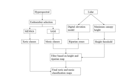
2.2. Methods
2.2.1. Classification
2.2.2. Classification Accuracy Assessment
3. Results
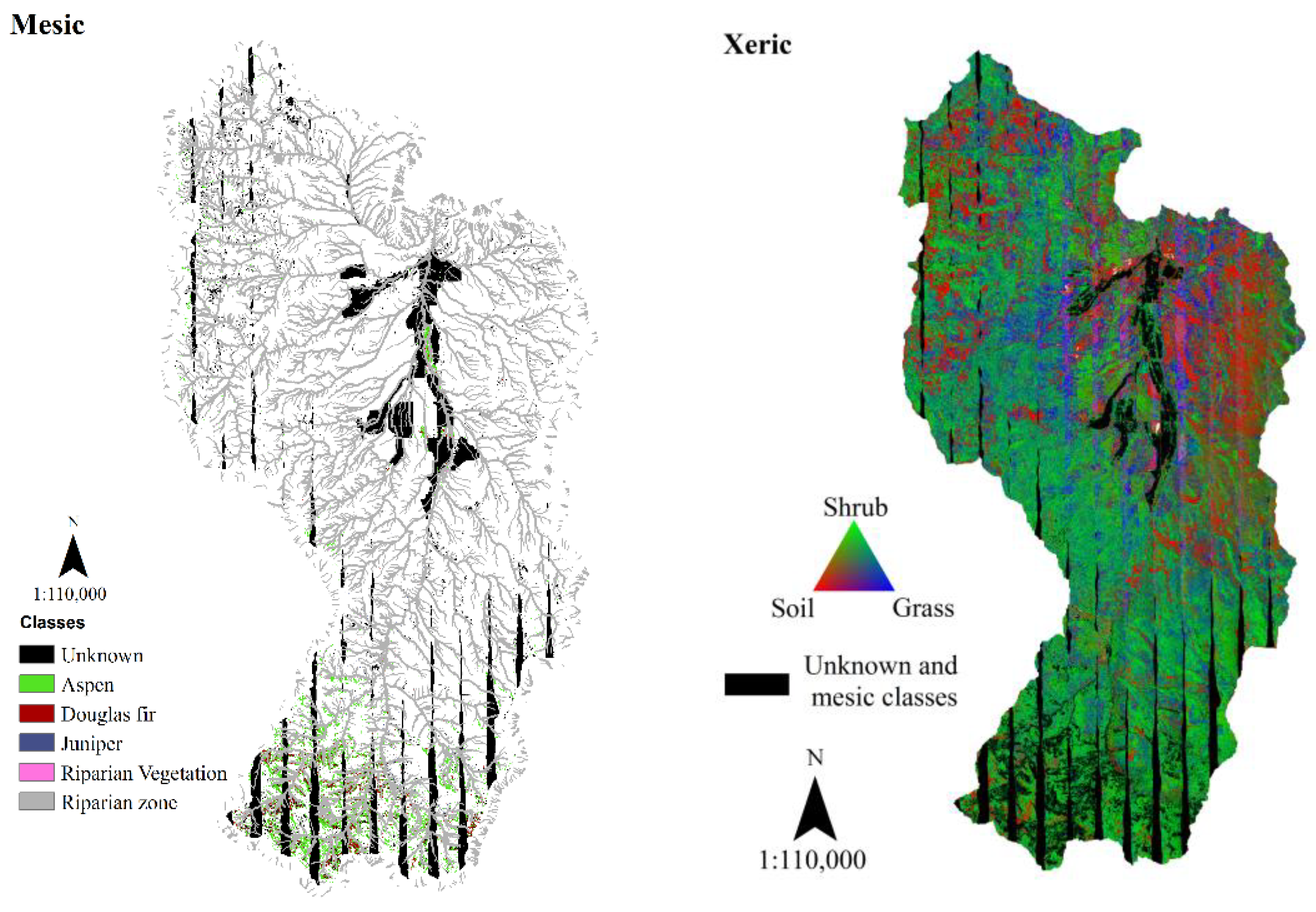
Classification
4. Discussion
4.1. Xeric Classification
4.2. Mesic Classification
5. Conclusions
Author Contributions
Funding
Acknowledgments
Conflicts of Interest
References
- Ahlström, A.; Raupach, M.R.; Schurgers, G.; Smith, B.; Arneth, A.; Jung, M.; Reichstein, M.; Canadell, J.G.; Friedlingstein, P.; Jain, A.K.; et al. The dominant role of semi-arid ecosystems in the trend and variability of the land CO2 sink. Science 2015, 348, 895–899. [Google Scholar] [CrossRef] [PubMed]
- Poulter, B.; Frank, D.; Ciais, P.; Myneni, R.B.; Andela, N.; Bi, J.; Broquet, G.; Canadell, J.G.; Chevallier, F.; Liu, Y.Y.; et al. Contribution of semi-arid ecosystems to interannual variability of the global carbon cycle. Natur 2014, 509, 600. [Google Scholar] [CrossRef] [PubMed]
- Dufour, A.; Gadallah, F.; Wagner, H.H.; Guisan, A.; Buttler, A. Plant Species Richness and Environmental Heterogeneity in a Mountain Landscape: Effects of Variability and Spatial Configuration. Ecography 2006, 29, 573–584. [Google Scholar] [CrossRef]
- Hofer, G.; Wagner, H.H.; Herzog, F.; Edwards, P.J. Effects of Topographic Variability on the Scaling of Plant Species Richness in Gradient Dominated Landscapes. Ecography 2008, 31, 131–139. [Google Scholar] [CrossRef]
- Adam, E.; Mutanga, O.; Rugege, D. Multispectral and hyperspectral remote sensing for identification and mapping of wetland vegetation: A review. Wetl. Ecol. Manag. 2010, 18, 281–296. [Google Scholar] [CrossRef]
- Asner, G.P.; Heidebrecht, K.B. Spectral unmixing of vegetation, soil and dry carbon cover in arid regions: Comparing multispectral and hyperspectral observations. Int. J. Remote Sens. 2002, 23, 3939–3958. [Google Scholar] [CrossRef]
- Ballanti, L.; Blesius, L.; Hines, E.; Kruse, B. Tree Species Classification Using Hyperspectral Imagery: A Comparison of Two Classifiers. Remote Sens. 2016, 8, 445. [Google Scholar] [CrossRef]
- George, R.; Padalia, H.; Kushwaha, S.P.S. Forest tree species discrimination in western Himalaya using EO-1 Hyperion. Int. J. Appl. Earth Obs. Geoinf. 2014, 28, 140–149. [Google Scholar] [CrossRef]
- Roth, K.L.; Roberts, D.A.; Dennison, P.E.; Alonzo, M.; Peterson, S.H.; Beland, M. Differentiating plant species within and across diverse ecosystems with imaging spectroscopy. Remote Sens. Environ. 2015, 167, 135–151. [Google Scholar] [CrossRef]
- Burai, P.; Deák, B.; Valkó, O.; Tomor, T. Classification of Herbaceous Vegetation Using Airborne Hyperspectral Imagery. Remote Sens. 2015, 7, 2046–2066. [Google Scholar] [CrossRef] [Green Version]
- Mitchell, J.J.; Glenn, N.; Anderson, M.; Hruska, R.C. Flight Considerations and Hyperspectral Image Classifications for Dryland Vegetation Management from a Fixed-wing UAS. Environ. Manag. Sustain. Dev. 2016, 5, 41–57. [Google Scholar] [CrossRef]
- Dashti, H.; Glenn, N.F.; Ustin, S.; Mitchell, J.J.; Qi, Y.; Ilangakoon, N.T.; Flores, A.N.; Silván-Cárdenas, J.L.; Zhao, K.; Spaete, L.P.; et al. Empirical Methods for Remote Sensing of Nitrogen in Drylands May Lead to Unreliable Interpretation of Ecosystem Function. IEEE Trans. Geosci. Remote Sens. 2019, 57, 3993–4004. [Google Scholar] [CrossRef]
- Silván-Cárdenas, J.L.; Wang, L. Retrieval of subpixel Tamarix canopy cover from Landsat data along the Forgotten River using linear and nonlinear spectral mixture models. Remote Sens. Environ. 2010, 114, 1777–1790. [Google Scholar] [CrossRef]
- Asner, G.P. Biophysical and Biochemical Sources of Variability in Canopy Reflectance. Remote Sens. Environ. 1998, 64, 234–253. [Google Scholar] [CrossRef]
- Hakkenberg, C.R.; Peet, R.K.; Urban, D.L.; Song, C. Modeling plant composition as community continua in a forest landscape with LiDAR and hyperspectral remote sensing. Ecol. Appl. 2018, 28, 177–190. [Google Scholar] [CrossRef] [PubMed]
- Ollinger, S.V. Sources of variability in canopy reflectance and the convergent properties of plants. New Phytol. 2011, 189, 375–394. [Google Scholar] [CrossRef] [PubMed]
- Roberts, D.A.; Ustin, S.L.; Ogunjemiyo, S.; Greenberg, J.; Dobrowski, S.Z.; Chen, J.; Hinckley, T.M. Spectral and Structural Measures of Northwest Forest Vegetation at Leaf to Landscape Scales. Ecosystems 2004, 7, 545–562. [Google Scholar] [CrossRef]
- Ustin, S.L.; Roberts, D.A.; Gamon, J.A.; Asner, G.P.; Green, R.O. Using Imaging Spectroscopy to Study Ecosystem Processes and Properties. Bioscience 2004, 54, 523–534. [Google Scholar] [CrossRef]
- Knyazikhin, Y.; Schull, M.A.; Stenberg, P.; Mõttus, M.; Rautiainen, M.; Yang, Y.; Marshak, A.; Carmona, P.L.; Kaufmann, R.K.; Lewis, P.; et al. Hyperspectral remote sensing of foliar nitrogen content. Proc. Natl. Acad. Sci. USA 2013, 110, E185–E192. [Google Scholar] [CrossRef]
- Wang, W.; Nemani, R.; Hashimoto, H.; Ganguly, S.; Huang, D.; Knyazikhin, Y.; Myneni, R.; Bala, G. An Interplay between Photons, Canopy Structure, and Recollision Probability: A Review of the Spectral Invariants Theory of 3D Canopy Radiative Transfer Processes. Remote Sens. 2018, 10, 1805. [Google Scholar] [CrossRef]
- Okin, G.S.; Roberts, D.A.; Murray, B.; Okin, W.J. Practical limits on hyperspectral vegetation discrimination in arid and semiarid environments. Remote Sens. Environ. 2001, 77, 212–225. [Google Scholar] [CrossRef]
- Roberts, D.A.; Gardner, M.; Church, R.; Ustin, S.; Scheer, G.; Green, R.O. Mapping Chaparral in the Santa Monica Mountains Using Multiple Endmember Spectral Mixture Models. Remote Sens. Environ. 1998, 65, 267–279. [Google Scholar] [CrossRef]
- Bioucas-Dias, J.M.; Plaza, A.; Dobigeon, N.; Parente, M.; Du, Q.; Gader, P.; Chanussot, J. Hyperspectral Unmixing Overview: Geometrical, Statistical, and Sparse Regression-Based Approaches. IEEE J. Sel. Top. Appl. Earth Obs. Remote Sens. 2012, 5, 354–379. [Google Scholar] [CrossRef] [Green Version]
- Borel, C.C.; Gerstl, S.A.W. Nonlinear spectral mixing models for vegetative and soil surfaces. Remote Sens. Environ. 1994, 47, 403–416. [Google Scholar] [CrossRef]
- Chang, C.-I.; Heinz, D.C. Constrained subpixel target detection for remotely sensed imagery. IEEE Trans. Geosci. Remote Sens. 2000, 38, 1144–1159. [Google Scholar] [CrossRef] [Green Version]
- Heinz, D.C. Fully constrained least squares linear spectral mixture analysis method for material quantification in hyperspectral imagery. IEEE Trans. Geosci. Remote Sens. 2001, 39, 529–545. [Google Scholar] [CrossRef] [Green Version]
- Li, X.; Jia, X.; Wang, L.; Zhao, K. On Spectral Unmixing Resolution Using Extended Support Vector Machines. IEEE Trans. Geosci. Remote Sens. 2015, 53, 4985–4996. [Google Scholar] [CrossRef]
- Ray, T.W.; Murray, B.C. Nonlinear spectral mixing in desert vegetation. Remote Sens. Environ. 1996, 55, 59–64. [Google Scholar] [CrossRef]
- Shanmugam, S.; SrinivasaPerumal, P. Spectral matching approaches in hyperspectral image processing. Int. J. Remote Sens. 2014, 35, 8217–8251. [Google Scholar] [CrossRef]
- Cho, M.A.; Debba, P.; Mathieu, R.; Naidoo, L.; van Aardt, J.; Asner, G.P. Improving Discrimination of Savanna Tree Species Through a Multiple-Endmember Spectral Angle Mapper Approach: Canopy-Level Analysis. IEEE Trans. Geosci. Remote Sens. 2010, 48, 4133–4142. [Google Scholar] [CrossRef]
- Yang, C.; Everitt, J.H.; Johnson, H.B. Applying image transformation and classification techniques to airborne hyperspectral imagery for mapping Ashe juniper infestations. Int. J. Remote Sens. 2009, 30, 2741–2758. [Google Scholar] [CrossRef]
- Dalponte, M.; Coomes, D.A. Tree-centric mapping of forest carbon density from airborne laser scanning and hyperspectral data. Methods Ecol. Evol. 2016, 7, 1236–1245. [Google Scholar] [CrossRef]
- Heinzel, J.; Koch, B. Exploring full-waveform LiDAR parameters for tree species classification. Int. J. Appl. Earth Obs. Geoinf. 2011, 13, 152–160. [Google Scholar] [CrossRef]
- Neuenschwander, A.L.; Magruder, L.A.; Tyler, M. Landcover classification of small-footprint, full-waveform lidar data. J. Appl. Remote Sens. 2009, 3, 1–13. [Google Scholar] [CrossRef]
- Vaughn, N.R.; Moskal, L.M.; Turnblom, E.C. Tree Species Detection Accuracies Using Discrete Point Lidar and Airborne Waveform Lidar. Remote Sens. 2012, 4, 377–403. [Google Scholar] [CrossRef] [Green Version]
- Glenn, N.F.; Spaete, L.P.; Sankey, T.T.; Derryberry, D.R.; Hardegree, S.P.; Mitchell, J.J. Errors in LiDAR-derived shrub height and crown area on sloped terrain. J. Arid Environ. 2011, 75, 377–382. [Google Scholar] [CrossRef]
- Mitchell, J.J.; Shrestha, R.; Spaete, L.P.; Glenn, N.F. Combining airborne hyperspectral and LiDAR data across local sites for upscaling shrubland structural information: Lessons for HyspIRI. Remote Sens. Environ. 2015, 167, 98–110. [Google Scholar] [CrossRef]
- Ilangakoon, N.T.; Glenn, N.F.; Dashti, H.; Painter, T.H.; Mikesell, T.D.; Spaete, L.P.; Mitchell, J.J.; Shannon, K. Constraining plant functional types in a semi-arid ecosystem with waveform lidar. Remote Sens. Environ. 2018, 209, 497–509. [Google Scholar] [CrossRef]
- Laslier, M.; Hubert-Moy, L.; Dufour, S. Mapping Riparian Vegetation Functions Using 3D Bispectral LiDAR Data. Water 2019, 11, 483. [Google Scholar] [CrossRef]
- Villarreal, M.L.; van Leeuwen, W.J.D.; Romo-Leon, J.R. Mapping and monitoring riparian vegetation distribution, structure and composition with regression tree models and post-classification change metrics. Int. J. Remote Sens. 2012, 33, 4266–4290. [Google Scholar] [CrossRef]
- Dowling, R.; Accad, A. Vegetation classification of the riparian zone along the Brisbane River, Queensland, Australia, using light detection and ranging (lidar) data and forward looking digital video. Can. J. Remote Sens. 2003, 29, 556–563. [Google Scholar] [CrossRef]
- Mielcarek, M.; Stereńczak, K.; Khosravipour, A. Testing and evaluating different LiDAR-derived canopy height model generation methods for tree height estimation. Int. J. Appl. Earth Obs. Geoinf. 2018, 71, 132–143. [Google Scholar] [CrossRef]
- Roussel, J.-R.; Caspersen, J.; Béland, M.; Thomas, S.; Achim, A. Removing bias from LiDAR-based estimates of canopy height: Accounting for the effects of pulse density and footprint size. Remote Sens. Environ. 2017, 198, 1–16. [Google Scholar] [CrossRef]
- Solomons, A.G.; Mikhailova, E.A.; Post, C.J.; Sharp, J.L. LiDAR-based predictions of flow channels through riparian buffer zones. Water Sci. 2015, 29, 123–133. [Google Scholar] [CrossRef] [Green Version]
- Tompalski, P.; Coops, N.C.; White, J.C.; Wulder, M.A.; Yuill, A. Characterizing streams and riparian areas with airborne laser scanning data. Remote Sens. Environ. 2017, 192, 73–86. [Google Scholar] [CrossRef]
- Glenn, N.F.; Neuenschwander, A.; Vierling, L.A.; Spaete, L.; Li, A.; Shinneman, D.J.; Pilliod, D.S.; Arkle, R.S.; McIlroy, S.K. Landsat 8 and ICESat-2: Performance and potential synergies for quantifying dryland ecosystem vegetation cover and biomass. Remote Sens. Environ. 2016, 185, 233–242. [Google Scholar] [CrossRef]
- Jeong, S.G.; Mo, Y.; Kim, H.G.; Park, C.H.; Lee, D.K. Mapping riparian habitat using a combination ofremote-sensing techniques. Int. J. Remote Sens. 2016, 37, 1069–1088. [Google Scholar] [CrossRef]
- Narine, L.L.; Popescu, C.S.; Malambo, L. Synergy of ICESat-2 and Landsat for Mapping Forest Aboveground Biomass with Deep Learning. Remote Sens. 2019, 11, 1503. [Google Scholar] [CrossRef]
- Zhang, Y.; Zhang, H.; Nasrabadi, N.M.; Huang, T.S. Multi-metric learning for multi-sensor fusion based classification. Inf. Fusion 2013, 14, 431–440. [Google Scholar] [CrossRef]
- Olsoy, P.J.; Mitchell, J.J.; Levia, D.F.; Clark, P.E.; Glenn, N.F. Estimation of big sagebrush leaf area index with terrestrial laser scanning. Ecol. Indic. 2016, 61 Pt 2, 815–821. [Google Scholar] [CrossRef]
- Spaete, L.P.; Glenn, N.F.; Derryberry, D.R.; Sankey, T.T.; Mitchell, J.J.; Hardegree, S.P. Vegetation and slope effects on accuracy of a LiDAR-derived DEM in the sagebrush steppe. Remote Sens. Lett. 2011, 2, 317–326. [Google Scholar] [CrossRef]
- Li, A.; Dhakal, S.; Glenn, F.N.; Spaete, P.L.; Shinneman, J.D.; Pilliod, S.D.; Arkle, S.R.; McIlroy, K.S. Lidar Aboveground Vegetation Biomass Estimates in Shrublands: Prediction, Uncertainties and Application to Coarser Scales. Remote Sensing 2017, 9, 903. [Google Scholar] [CrossRef]
- Seyfried, M.; Harris, R.; Marks, D.; Jacob, B. Geographic Database, Reynolds Creek Experimental Watershed, Idaho, United States. Water Resour. Res. 2001, 37, 2825–2829. [Google Scholar] [CrossRef] [Green Version]
- Pyke, D.A.; Chambers, J.C.; Pellant, M.; Knick, S.T.; Miller, R.F.; Beck, J.L.; Doescher, P.S.; Schupp, E.W.; Roundy, B.A.; Brunson, M.; et al. Restoration Handbook for Sagebrush Steppe Ecosystems with Emphasis on Greater Sage-Grouse Habitat—Part 1. Concepts for Understanding and Applying Restoration; US Geological Survey: Reston, VA, USA, 2015. [Google Scholar]
- Council, N.R. Riparian Areas: Functions and Strategies for Management; The National Academies Press: Washington, DC, USA, 2002. [Google Scholar]
- Booth, D.T.; Cox, S.E.; Berryman, R.D. Point Sampling Digital Imagery with ‘Samplepoint’. Environ. Monit. Assess. 2006, 123, 97–108. [Google Scholar] [CrossRef]
- Gao, B.-C.; Montes, M.J.; Davis, C.O.; Goetz, A.F.H. Atmospheric correction algorithms for hyperspectral remote sensing data of land and ocean. Remote Sens. Environ. 2009, 113, S17–S24. [Google Scholar] [CrossRef]
- Roberts, D.A.; Halligan, K.; Dennison, P. VIPER Tools User Manual; 2007. Available online: https://bitbucket.org/kul-reseco/viper (accessed on 11 September 2019).
- Dennison, P.E.; Halligan, K.Q.; Roberts, D.A. A comparison of error metrics and constraints for multiple endmember spectral mixture analysis and spectral angle mapper. Remote Sens. Environ. 2004, 93, 359–367. [Google Scholar] [CrossRef]
- Dennison, P.E.; Roberts, D.A. Endmember selection for multiple endmember spectral mixture analysis using endmember average RMSE. Remote Sens. Environ. 2003, 87, 123–135. [Google Scholar] [CrossRef]
- Streutker, D.R.; Glenn, N.F. LiDAR measurement of sagebrush steppe vegetation heights. Remote Sens. Environ. 2006, 102, 135–145. [Google Scholar] [CrossRef]
- Montgomery, D.R.; Dietrich, W.E. Channel Initiation and the Problem of Landscape Scale. Science 1992, 255, 826–830. [Google Scholar] [CrossRef] [Green Version]
- Salo, J.A.; Theobald, D.M.; Brown, T.C. Evaluation of Methods for Delineating Riparian Zones in a Semi-Arid Montane Watershed. JAWRA J. Am. Water Resour. Assoc. 2016, 52, 632–647. [Google Scholar] [CrossRef]
- Li, Y.; Nigh, T. GIS-based prioritization of private land parcels for biodiversity conservation: A case study from the Current and Eleven Point Conservation Opportunity Areas, Missouri. Appl. Geogr. 2011, 31, 98–107. [Google Scholar] [CrossRef]
- Silván-Cárdenas, J.L.; Wang, L. Sub-pixel confusion–uncertainty matrix for assessing soft classifications. Remote Sens. Environ. 2008, 112, 1081–1095. [Google Scholar] [CrossRef]
- Patel, N.; Kaushal, B. Improvement of user’s accuracy through classification of principal component images and stacked temporal images. Geo-Spat. Inf. Sci. 2010, 13, 243–248. [Google Scholar] [CrossRef]
- David, R.; Patricia, H.; Karen, E.; Susan, G.; Juliet, S.; Steven, K.; Petr, P.; Richard, H. Riparian vegetation: Degradation, alien plant invasions, and restoration prospects. Divers. Distrib. 2007, 13, 126–139. [Google Scholar]
- Patten, D.T. Riparian ecosytems of semi-arid North America: Diversity and human impacts. Wetlands 1998, 18, 498–512. [Google Scholar] [CrossRef]
- Huang, D.; Knyazikhin, Y.; Dickinson, R.E.; Rautiainen, M.; Stenberg, P.; Disney, M.; Lewis, P.; Cescatti, A.; Tian, Y.; Verhoef, W.; et al. Canopy spectral invariants for remote sensing and model applications. Remote Sens. Environ. 2007, 106, 106–122. [Google Scholar] [CrossRef] [Green Version]
- Arroyo, L.A.; Johansen, K.; Armston, J.; Phinn, S. Integration of LiDAR and QuickBird imagery for mapping riparian biophysical parameters and land cover types in Australian tropical savannas. For. Ecol. Manag. 2010, 259, 598–606. [Google Scholar] [CrossRef]
- Hall, R.K.; Watkins, R.L.; Heggem, D.T.; Jones, K.B.; Kaufmann, P.R.; Moore, S.B.; Gregory, S.J. Quantifying structural physical habitat attributes using LIDAR and hyperspectral imagery. Environ. Monit. Assess. 2009, 159, 63. [Google Scholar] [CrossRef]
- Wasser, L.; Day, R.; Chasmer, L.; Taylor, A. Influence of Vegetation Structure on Lidar-derived Canopy Height and Fractional Cover in Forested Riparian Buffers During Leaf-Off and Leaf-On Conditions. PLoS ONE 2013, 8, e54776. [Google Scholar] [CrossRef]
- Ghamisi, P.; Höfle, B.; Zhu, X.X. Hyperspectral and LiDAR Data Fusion Using Extinction Profiles and Deep Convolutional Neural Network. IEEE J. Sel. Top. Appl. Earth Obs. Remote Sens. 2017, 10, 3011–3024. [Google Scholar] [CrossRef]
- Xu, X.; Li, W.; Ran, Q.; Du, Q.; Gao, L.; Zhang, B. Multisource Remote Sensing Data Classification Based on Convolutional Neural Network. IEEE Trans. Geosci. Remote Sens. 2018, 56, 937–949. [Google Scholar] [CrossRef]
- Dalponte, M.; Bruzzone, L.; Gianelle, D. Fusion of Hyperspectral and LIDAR Remote Sensing Data for Classification of Complex Forest Areas. IEEE Trans. Geosci. Remote Sens. 2008, 46, 1416–1427. [Google Scholar] [CrossRef] [Green Version]
- Liao, W.; Pižurica, A.; Bellens, R.; Gautama, S.; Philips, W. Generalized Graph-Based Fusion of Hyperspectral and LiDAR Data Using Morphological Features. IEEE Geosci. Remote Sens. Lett. 2015, 12, 552–556. [Google Scholar] [CrossRef]
- Asner, G.P.; Knapp, D.E.; Kennedy-Bowdoin, T.; Jones, M.O.; Martin, R.E.; Boardman, J.; Hughes, R.F. Invasive species detection in Hawaiian rainforests using airborne imaging spectroscopy and LiDAR. Remote Sens. Environ. 2008, 112, 1942–1955. [Google Scholar] [CrossRef]
- Koetz, B.; Morsdorf, F.; van der Linden, S.; Curt, T.; Allgöwer, B. Multi-source land cover classification for forest fire management based on imaging spectrometry and LiDAR data. For. Ecol. Manag. 2008, 256, 263–271. [Google Scholar] [CrossRef]
- Liao, W.; Bellens, R.; Pižurica, A.; Gautama, S.; Philips, W. Combining feature fusion and decision fusion for classification of hyperspectral and LiDAR data. In Proceedings of the 2014 IEEE Geoscience and Remote Sensing Symposium, Quebec City, QC, Canada, 13–18 July 2014; pp. 1241–1244. [Google Scholar]
- Degerickx, J.; Roberts, D.A.; Somers, B. Enhancing the performance of Multiple Endmember Spectral Mixture Analysis (MESMA) for urban land cover mapping using airborne lidar data and band selection. Remote Sens. Environ. 2019, 221, 260–273. [Google Scholar] [CrossRef]
- Zhi, W.; Yuan, L.; Ji, G.; Liu, Y.; Cai, Z.; Chen, X. A bibliometric review on carbon cycling research during 1993–2013. Environ. Earth Sci. 2015, 74, 6065–6075. [Google Scholar] [CrossRef]
- Bateson, C.A.; Asner, G.P.; Wessman, C.A. Endmember bundles: A new approach to incorporating endmember variability into spectral mixture analysis. IEEE Trans. Geosci. Remote Sens. 2000, 38, 1083–1094. [Google Scholar] [CrossRef]
- Deng, C. Incorporating Endmember Variability into Linear Unmixing of Coarse Resolution Imagery: Mapping Large-Scale Impervious Surface Abundance Using a Hierarchically Object-Based Spectral Mixture Analysis. Remote Sens. 2015, 7, 9205–9229. [Google Scholar] [CrossRef] [Green Version]
- Disney, M. Remote Sensing of Vegetation: Potentials, Limitations, Developments and Applications. In Canopy Photosynthesis: From Basics to Applications; Hikosaka, K., Niinemets, Ü., Anten, N.P.R., Eds.; Springer: Dordrecht, The Netherlands, 2016; pp. 289–331. [Google Scholar]
- Hall, F.G.; Hilker, T.; Coops, N.C.; Lyapustin, A.; Huemmrich, K.F.; Middleton, E.; Margolis, H.; Drolet, G.; Black, T.A. Multi-angle remote sensing of forest light use efficiency by observing PRI variation with canopy shadow fraction. Remote Sens. Environ. 2008, 112, 3201–3211. [Google Scholar] [CrossRef] [Green Version]
- Hancock, S.; Armston, J.; Hofton, M.; Sun, X.; Tang, H.; Duncanson, L.I.; Kellner, J.R.; Dubayah, R. The GEDI Simulator: A Large-Footprint Waveform Lidar Simulator for Calibration and Validation of Spaceborne Missions. Earth Space Sci. 2019, 6, 294–310. [Google Scholar] [CrossRef]
- Svejcar, T.; Boyd, C.; Davies, K.; Hamerlynck, E.; Svejcar, L. Challenges and limitations to native species restoration in the Great Basin, USA. Plant Ecol. 2017, 218, 81–94. [Google Scholar] [CrossRef]
- Arkle, R.S.; Pilliod, D.S.; Hanser, S.E.; Brooks, M.L.; Chambers, J.C.; Grace, J.B.; Knutson, K.C.; Pyke, D.A.; Welty, J.L.; Wirth, T.A. Quantifying restoration effectiveness using multi-scale habitat models: Implications for sage-grouse in the Great Basin. Ecosphere 2014, 5, art31. [Google Scholar] [CrossRef]
- Donnelly, J.P.; Naugle, D.E.; Hagen, C.A.; Maestas, J.D. Public lands and private waters: Scarce mesic resources structure land tenure and sage-grouse distributions. Ecosphere 2016, 7, e01208. [Google Scholar] [CrossRef]
- Flerchinger, G.N.; Fellows, A.W.; Seyfried, M.S.; Clark, P.E.; Lohse, K.A. Water and Carbon Fluxes Along an Elevational Gradient in a Sagebrush Ecosystem. Ecosystems 2019, 1–18. [Google Scholar] [CrossRef]
- Renwick, K.M.; Fellows, A.; Flerchinger, G.N.; Lohse, K.A.; Clark, P.E.; Smith, W.K.; Emmett, K.; Poulter, B. Modeling phenological controls on carbon dynamics in dryland sagebrush ecosystems. Agric. For. Meteorol. 2019, 274, 85–94. [Google Scholar] [CrossRef]


| Classes | Image Extracted EM | EM Used in Final Classification | Validation Samples |
|---|---|---|---|
| Aspen | 1004 | 3 | 4816 |
| Douglas fir | 90 | 3 | 3947 |
| Juniper | 187 | 3 | 1409 |
| Riparian | 1316 | 5 | 3271 |
| Shrub | 328 | 7 | 3400 |
| Grass | 464 | 2 | 3400 |
| Soil | 100 | 3 | 3400 |
| Class | User’s Accuracy | Producer’s Accuracy |
|---|---|---|
| Shrub | 0.59 | 0.99 |
| Grass | 0.76 | 0.79 |
| Soil | 0.99 | 0.35 |
| Overall accuracy = 0.67 | ||
| Ground Reference | Accuracy | |||||||
|---|---|---|---|---|---|---|---|---|
| Aspen | Riparian | Douglas Fir | Juniper | Total | User’s Accuracy | Producer’s Accuracy | ||
| Classified | Aspen | 2015 | 553 | 398 | 66 | 3032 | 0.66 | 0.44 |
| Riparian | 2411 | 1806 | 130 | 5 | 4352 | 0.41 | 0.63 | |
| Douglas fir | 95 | 500 | 2014 | 100 | 2709 | 0.74 | 0.77 | |
| Juniper | 7 | 0 | 46 | 636 | 689 | 0.92 | 0.78 | |
| Total | 4528 | 2859 | 2588 | 807 | 10782 | --- | --- | |
| Overall accuracy = 0.60 | ||||||||
| Classified incorporating lidar | Aspen | 4298 | 128 | 398 | 66 | 4890 | 0.87 | 0.94 |
| Riparian | 129 | 2718 | 130 | 5 | 2982 | 0.91 | 0.95 | |
| Douglas fir | 94 | 13 | 2014 | 100 | 2221 | 0.90 | 0.77 | |
| Juniper | 7 | 0 | 46 | 636 | 689 | 0.92 | 0.78 | |
| Total | 4528 | 2859 | 2588 | 807 | 10782 | --- | --- | |
| Overall accuracy = 0.89 | ||||||||
© 2019 by the authors. Licensee MDPI, Basel, Switzerland. This article is an open access article distributed under the terms and conditions of the Creative Commons Attribution (CC BY) license (http://creativecommons.org/licenses/by/4.0/).
Share and Cite
Dashti, H.; Poley, A.; F. Glenn, N.; Ilangakoon, N.; Spaete, L.; Roberts, D.; Enterkine, J.; N. Flores, A.; L. Ustin, S.; J. Mitchell, J. Regional Scale Dryland Vegetation Classification with an Integrated Lidar-Hyperspectral Approach. Remote Sens. 2019, 11, 2141. https://doi.org/10.3390/rs11182141
Dashti H, Poley A, F. Glenn N, Ilangakoon N, Spaete L, Roberts D, Enterkine J, N. Flores A, L. Ustin S, J. Mitchell J. Regional Scale Dryland Vegetation Classification with an Integrated Lidar-Hyperspectral Approach. Remote Sensing. 2019; 11(18):2141. https://doi.org/10.3390/rs11182141
Chicago/Turabian StyleDashti, Hamid, Andrew Poley, Nancy F. Glenn, Nayani Ilangakoon, Lucas Spaete, Dar Roberts, Josh Enterkine, Alejandro N. Flores, Susan L. Ustin, and Jessica J. Mitchell. 2019. "Regional Scale Dryland Vegetation Classification with an Integrated Lidar-Hyperspectral Approach" Remote Sensing 11, no. 18: 2141. https://doi.org/10.3390/rs11182141