Environmental Differences between Migratory and Resident Ungulates—Predicting Movement Strategies in Rocky Mountain Mule Deer (Odocoileus hemionus) with Remotely Sensed Plant Phenology, Snow, and Land Cover

 , ,
, ,
Abstract
:
1. Introduction
2. Methods
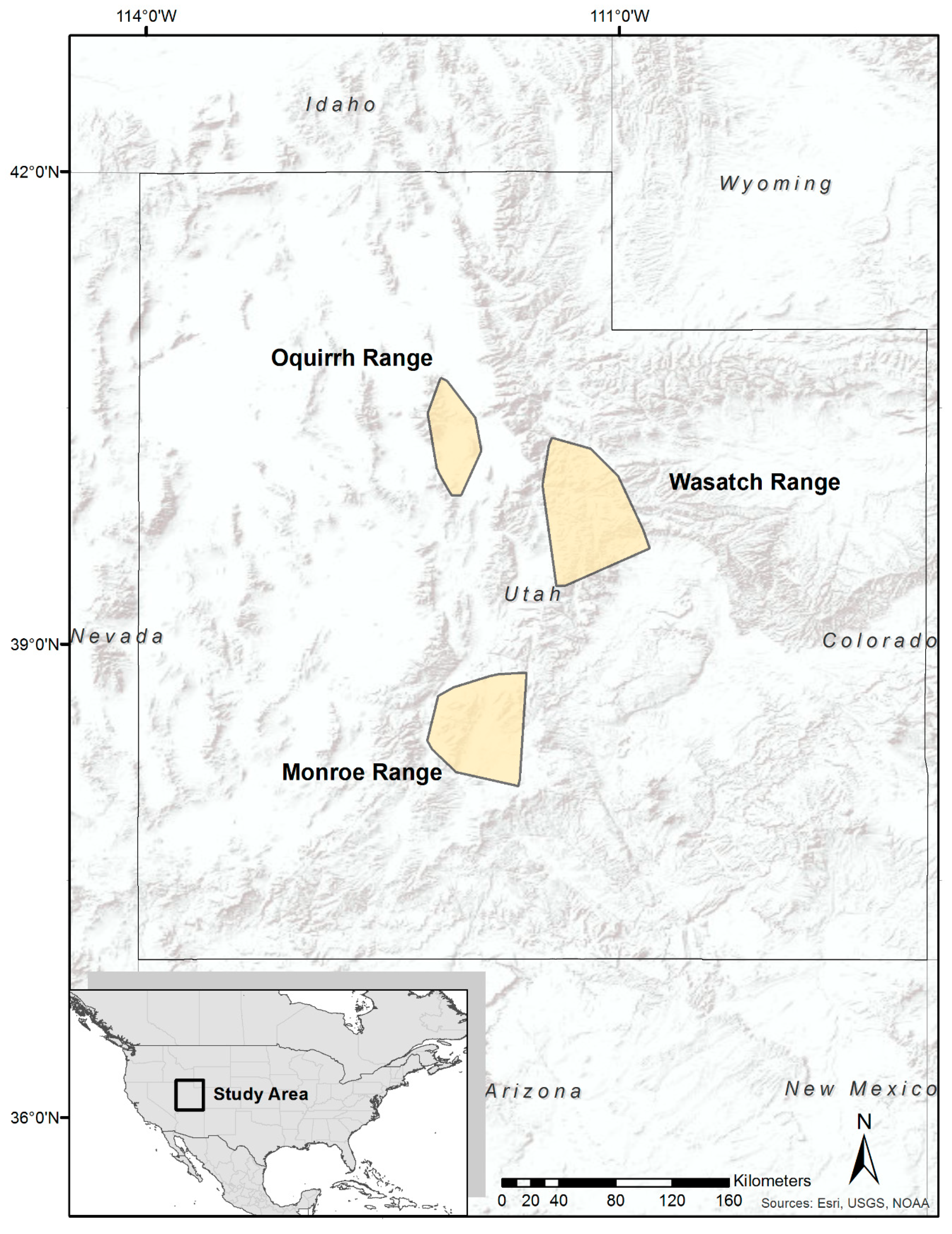
2.1. Study Area
2.2. Animal Locations and Migratory Habitat
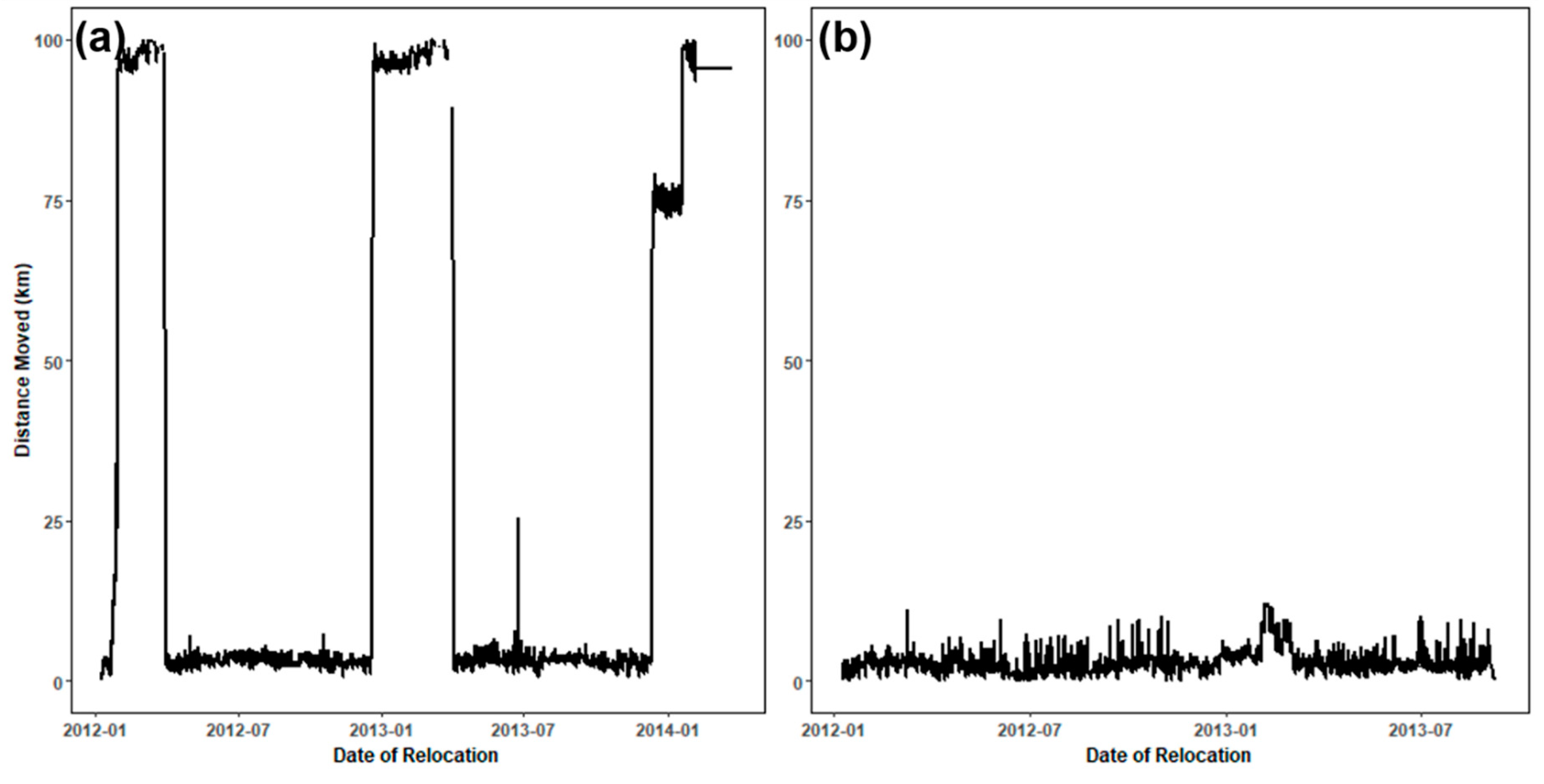
2.3. Classification of Movement Points
2.4. Predictive Environmental Variables
2.5. Model Setup
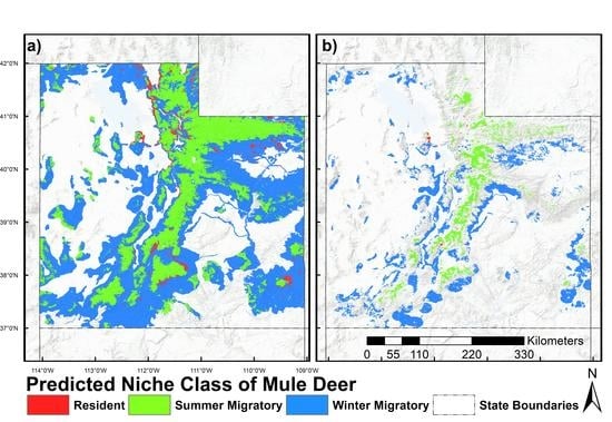
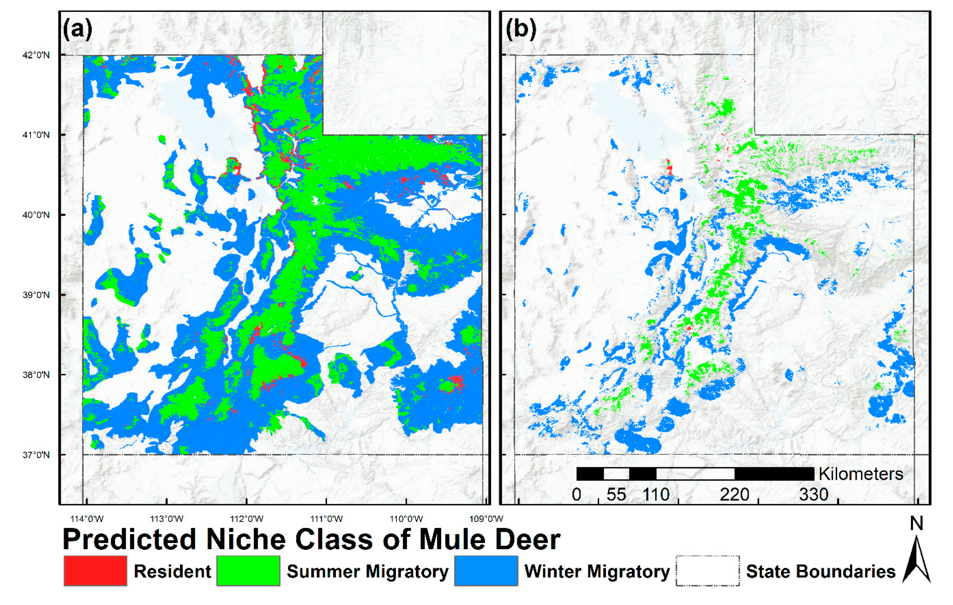
2.6. Prediction and Mapping Migratory/Resident Niches
3. Results
4. Discussion
5. Conclusions
Supplementary Materials
Author Contributions
Funding
Acknowledgments
Conflicts of Interest
References
- Fryxell, J.M.; Greever, J.; Sinclair, A.R.E. Why are migratory ungulates so abundant? Am. Nat. 1988, 131, 781–798. [Google Scholar] [CrossRef]
- Mueller, T.; Olson, K.A.; Dressler, G.; Leimgruber, P.; Fuller, T.K.; Nicolson, C.; Novaro, A.J.; Bolgeri, M.J.; Wattles, D.; DeStefano, S.; et al. How landscape dynamics link individual-to population-level movement patterns: A multispecies comparison of ungulate relocation data. Glob. Ecol. Biogeogr. 2011, 20, 683–684. [Google Scholar] [CrossRef]
- Bischof, R.; Loe, L.E.; Meisingset, E.L.; Zimmermann, B.; Van Moorter, B.; Mysterud, A. A migratory northern ungulate in the pursuit of spring: Jumping or surfing the green wave? Am. Nat. 2012, 180, 407–424. [Google Scholar] [CrossRef] [PubMed]
- Merkle, J.A.; Monteith, K.L.; Aikens, E.O.; Hayes, M.M.; Hersey, K.R.; Middleton, A.D.; Oates, B.A.; Sawyer, H.; Scurlock, B.M.; Kauffman, M.J. Large herbivores surf waves of green-up in spring. Proc. R. Soc. B 2016, 283, 20160456. [Google Scholar] [CrossRef] [PubMed]
- Lundberg, P. The evolution of partial migration in Birds. Trends Ecol. Evol. 1988, 3, 172–175. [Google Scholar] [CrossRef]
- Newton, I.; Dale, L.C. Bird migration at different latitudes in eastern North America. Auk 1996, 113, 626–635. [Google Scholar] [CrossRef]
- Newton, I.; Dale, L. Relationship between migration and latitude among west European birds. J. Anim. Ecol. 1996, 65, 137–146. [Google Scholar] [CrossRef]
- Singh, N.J.; Börger, L.; Dettki, H.; Bunnefeld, N.; Ericsson, G. From migration to nomadism: Movement variability in a northern ungulate across its latitudinal range. Ecol. Appl. 2012, 22, 2007–2020. [Google Scholar] [CrossRef]
- Berger, J. The last mile: How to sustain long-distance migration in mammals. Conserv. Biol. 2004, 18, 320–331. [Google Scholar] [CrossRef]
- Bolger, D.T.; Newmark, W.D.; Morrison, T.A.; Doak, D.F. The need for integrative approaches to understand and conserve migratory ungulates. Ecol. Lett. 2008, 11, 63–77. [Google Scholar] [CrossRef]
- Harris, G.; Thirgood, S.; Hopcraft, J.G.C.; Cromsigt, J.P.G.M.; Berger, J. Global decline in aggregated migrations of large terrestrial mammals. Endanger. Species Res. 2009, 7, 55–76. [Google Scholar] [CrossRef]
- Hebblewhite, M.; Merrill, E.H. Demographic balancing of migrant and resident elk in a partially migratory population through forage-predation tradeoffs. Oikos 2011, 120, 1860–1870. [Google Scholar] [CrossRef]
- Middleton, A.D.; Kauffman, M.J.; Mcwhirter, D.E.; Cook, J.G.; Cook, R.C.; Nelson, A.A.; Jimenez, M.D.; Klaver, R.W. Animal migration amid shifting patterns of phenology and predation: Lessons from a Yellowstone elk herd. Ecology 2013, 94, 1245–1256. [Google Scholar] [CrossRef] [PubMed]
- Middleton, A.D.; Merkle, J.A.; Mcwhirter, D.E.; Cook, J.G.; Cook, R.C.; White, P.J.; Kauffman, M.J. Green-wave surfing increases fat gain in a migratory ungulate. Oikos 2018, 127, 1060–1068. [Google Scholar] [CrossRef]
- Farnsworth, M.L.; Wolfe, L.L.; Hobbs, N.T.; Burnham, K.P.; Williams, E.S.; Theobald, D.M.; Conner, M.M.; Miller, M.W. Human land use influences chronic wasting disease prevalence in mule deer. Ecol. Appl. 2005, 15, 119–126. [Google Scholar] [CrossRef]
- Jesmer, B.R.; Goheen, J.R.; Aikens, E.O.; Merkle, J.A.; Monteith, K.L.; Beck, J.L.; Courtemanch, A.B.; McWhirter, D.E.; Hurley, M.A.; Miyasaki, H.M.; et al. Is ungulate migration culturally transmitted? Evidence of social learning from translocated animals. Science 2018, 361, 1023–1025. [Google Scholar] [CrossRef] [PubMed] [Green Version]
- Caro, T.; Sherman, P.W. Vanishing behaviors. Conserv. Lett. 2012, 5, 159–166. [Google Scholar] [CrossRef]
- Caro, T. Behavior and conservation: A bridge too far? Trends Ecol. Evol. 2007, 22, 394–400. [Google Scholar] [CrossRef]
- Brown, D.G.; Johnson, K.M.; Loveland, T.R.; Theobald, D.M. Rural land-use trends in the conterminous United States, 1950–2000. Ecol. Appl. 2005, 15, 1851–1863. [Google Scholar] [CrossRef]
- Sawyer, H.; Kauffman, M.J.; Nielson, R.M. Influence of well pad activity on winter habitat selection patterns of mule deer. J. Wildl. Manag. 2009, 73, 1052–1061. [Google Scholar] [CrossRef]
- Wyckoff, T.B.; Sawyer, H.; Albeke, S.E.; Garman, S.L.; Kauffman, M.J. Evaluating the influence of energy and residential development on the migratory behavior of mule deer. Ecosphere 2018, 9, e02113. [Google Scholar] [CrossRef]
- Fryxell, J.M.; Sinclair, A.R.E. Causes and consequences of migration by large herbivores. Trends Ecol. Evol. 1988, 3, 237–241. [Google Scholar] [CrossRef]
- Utah Division of Wildlife Resources Utah Statewide Management Plan for Mule Deer; Utah Division of Wildlife Resources: Salt Lake City, UT, USA, 2014.
- Department of the Interior Order No. 3362: Improving Habitat Quality in Western Big-Game Winter Range and Migration Corridors; United States Department of Interior: Washington, DC, USA, 2018.
- Colwell, R.K.; Rangel, T.F. Hutchinson’s duality: The once and future niche. Proc. Natl. Acad. Sci. USA 2009, 106, 19651–19658. [Google Scholar] [CrossRef] [PubMed]
- Hutchinson, G.E. Concluding Remarks. Cold Spring Harb. Symp. Quant. Biol. 1957, 22, 415–427. [Google Scholar] [CrossRef]
- Sawyer, H.; Merkle, J.A.; Middleton, A.D.; Dwinnell, S.P.H.; Monteith, K.L. Migratory plasticity is not ubiquitous among large herbivores. J. Anim. Ecol. 2019, 88, 450–460. [Google Scholar] [CrossRef] [PubMed]
- Stoner, D.C.; Sexton, J.O.; Nagol, J.; Bernales, H.H.; Edwards, T.C. Ungulate reproductive parameters track satellite observations of plant phenology across latitude and climatological regimes. PLoS ONE 2016, 11, e0148780. [Google Scholar] [CrossRef] [PubMed]
- Stoner, D.C.; Sexton, J.O.; Choate, D.M.; Nagol, J.; Bernales, H.H.; Sims, S.A.; Ironside, K.E.; Longshore, K.M.; Edwards, T.C. Climatically driven changes in primary production propagate through trophic levels. Glob. Chang. Biol. 2018, 24, 4453–4463. [Google Scholar] [CrossRef] [Green Version]
- Jarvis, A.; Reuter, H.I.; Nelson, A.; Guevara, E. Hole-Filled SRTM for the Globe Version 4. CGIAR-CSI SRTM 90 m Database. 2008. Available online: http://srtm.csi.cgiar.org (accessed on 21 August 2019).
- Banner, R.E.; Baldwin, B.D.; McGinty, E.L. Rangeland Resources of Utah; Utah State University: Logan, UT, USA, 2009. [Google Scholar]
- Bradley, B.A.; Mustard, J.F. Comparison of phenology trends by land cover class: A case study in the Great Basin, USA. Glob. Chang. Biol. 2008, 14, 334–346. [Google Scholar] [CrossRef]
- Travis, W.R. New Geographies of the American West: Land Use and the Changing Patterns of Place; Island Press: Washington, DC, USA, 2007. [Google Scholar]
- Olson, D.D. Assessing Vehicle-Related Mortality of Mule Deer in Utah. Ph.D. Thesis, Utah State University, Logan, UT, USA, 2013. [Google Scholar]
- Papworth, S.K.; Bunnefeld, N.; Slocombe, K.; Milner-Gulland, E.J. Movement ecology of human resource users: Using net squared displacement, biased random bridges and resource utilization functions to quantify hunter and gatherer behaviour. Methods Ecol. Evol. 2012, 3, 584–594. [Google Scholar] [CrossRef]
- Rouse, J.W.; Hass, R.H.; Schell, J.A.; Deering, D.W. Monitoring vegetation systems in the great plains with ERTS. In Third Earth Resources Technology Satellite-1 Symposium—Volume I: Technical Presentations; NASA: Washington, DC, USA, 1974; Volume 1, pp. 309–317. [Google Scholar]
- Tucker, C. Red and photographic infrared linear combinations for monitoring vegetation. Remote Sens. Environ. 1979, 8, 127–150. [Google Scholar] [CrossRef] [Green Version]
- Didan, K. MOIDS/Terra Vegetation Indices 16-Day L3 Global 250 m SIN Grid V006. 2015. Available online: https://lpdaac.usgs.gov/products/mod13q1v006/ (accessed on 21 August 2019).
- Pettorelli, N.; Ryan, S.; Mueller, T.; Bunnefeld, N.; Jedrzejewska, B.; Lima, M.; Kausrud, K. The Normalized Difference Vegetation Index (NDVI): Unforeseen successes in animal ecology. Clim. Res. 2011, 46, 15–27. [Google Scholar] [CrossRef]
- Nolin, A.W. Recent advances in remote sensing of seasonal snow. J. Glaciol. 2011, 56, 1141–1150. [Google Scholar] [CrossRef]
- Hall, D.K.; Riggs, G.A. MODIS/Terra Snow Cover Daily L3 Global 500 m GRID, Version 6. 2016. Available online: https://nsidc.org/data/mod10a1 (accessed on 21 August 2019).
- Monteith, K.L.; Bleich, V.C.; Stephenson, T.R.; Pierce, B.M.; Conner, M.M.; Kie, J.G.; Bowyer, R.T. Life-history characteristics of mule deer: Effects of nutrition in a variable environment. Wildl. Monogr. 2014, 186, 1–62. [Google Scholar] [CrossRef]
- Nicholson, M.C.; Bowyer, R.T.; Kie, J.G. Habitat selection and survival of mule deer: Tradeoffs associated with migration. J. Mammal. 1997, 78, 483–504. [Google Scholar] [CrossRef]
- Rivrud, I.M.; Loe, L.E.; Mysterud, A. How does local weather predict red deer home range size at different temporal scales? J. Anim. Ecol. 2010, 79, 1280–1295. [Google Scholar] [CrossRef]
- Sawyer, H.; Kauffman, M.J. Stopover ecology of a migratory ungulate. J. Anim. Ecol. 2011, 80, 1078–1087. [Google Scholar] [CrossRef] [PubMed]
- Homer, C.; Dewitz, J.; Yang, L.; Jin, S.; Danielson, P.; Xian, G.; Coulston, J.; Herold, N.; Wickham, J.; Megown, K. Completion of the 2011 National Land Cover Database for the conterminous United States-representing a decade of land cover change information. Photogramm. Eng. Remote Sens. 2015, 81, 345–354. [Google Scholar]
- Breiman, L. Random forests. Mach. Learn. 2001, 45, 5–32. [Google Scholar] [CrossRef]
- Cutler, D.R.; Edwards, T.C.; Beard, K.H.; Cutler, A.; Hess, K.T.; Gibson, J.; Lawler, J.J. Random Forests for Classification in Ecology. Ecology 2007, 88, 2783–2792. [Google Scholar] [CrossRef]
- Strobl, C.; Boulesteix, A.L.; Kneib, T.; Augustin, T.; Zeileis, A. Conditional variable importance for random forests. BMC Bioinform. 2008, 9, 307. [Google Scholar] [CrossRef]
- Utah Division of Wildlife Resources Habitat Coverages: Mule Deer Habitat. 2015. Available online: https://dwrcdc.nr.utah.gov/ucdc/ (accessed on 21 August 2019).
- R Core Team. R: A Language and Environment for Statistical Computing; R Core Team: Vienna, Austria, 2016. [Google Scholar]
- Liaw, A.; Wiener, M. Classification and Regression by randomForest. R News 2002, 2, 18–22. [Google Scholar]
- Sawyer, H.; Lindzey, F.; McWhirter, D. Mule deer and pronghorn migration in western Wyoming. Wildl. Soc. Bull. 2005, 33, 1266–1273. [Google Scholar] [CrossRef]
- Barker, K.J.; Mitchell, M.S.; Proffitt, K.M.; DeVoe, J.D. Land management alters traditional nutritional benefits of migration for elk. J. Wildl. Manag. 2019, 83, 167–174. [Google Scholar] [CrossRef]
- Vogel, W.O. Response of deer to density and distribution of housing in Montana. Wildl. Soc. Bull. 1989, 17, 406–413. [Google Scholar]
- Anderson, E.D.; Long, R.A.; Atwood, M.P.; Kie, J.G.; Thomas, T.R.; Zager, P.; Bowyer, R.T. Winter resource selection by female mule deer Odocoileus hemionus: Functional response to spatio-temporal changes in habitat. Wildl. Biol. 2012, 18, 153–163. [Google Scholar] [CrossRef]
- Tucker, M.A.; Böhning-gaese, K.; Fagan, W.F.; Fryxell, J.M.; Van Moorter, B.; Alberts, S.C.; Ali, A.H.; Allen, A.M.; Attias, N.; Avgar, T.; et al. Moving in the Anthropocene: Global reductions in terrestrial mammalian movements. Science 2018, 359, 466–469. [Google Scholar] [CrossRef] [PubMed] [Green Version]
- Bracis, C.; Mueller, T. Memory, not just perception, plays an important role in terrestrial mammalian migration. Proc. R. Soc. B Biol. Sci. 2017, 284. [Google Scholar] [CrossRef] [PubMed]
- Garrott, R.A.; White, G.C.; Bartmann, R.M.; Carpenter, L.H.; Alldredge, A.W. Movements of female mule deer in northwest Colorado. J. Wildl. Manag. 1987, 51, 634–643. [Google Scholar] [CrossRef]
- Aikens, E.O.; Kauffman, M.J.; Merkle, J.A.; Dwinnell, S.P.H.; Fralick, G.L.; Monteith, K.L. The greenscape shapes surfing of resource waves in a large migratory herbivore. Ecol. Lett. 2017, 20, 741–750. [Google Scholar] [CrossRef]
- Fensholt, R.; Sandholt, I.; Rasmussen, M.S. Evaluation of MODIS LAI, fAPAR and the relation between fAPAR and NDVI in a semi-arid environment using in situ measurements. Remote Sens. Environ. 2004, 91, 490–507. [Google Scholar] [CrossRef]
- Mueller, T.; Fagan, W.F. Search and navigation in dynamic environments—From individual behaviours to population distributions. Oikos 2008, 117, 654–664. [Google Scholar] [CrossRef]


| Variable Name | Class of Variable | Description and Data Source |
|---|---|---|
| NDVI January–December | Phenology | The average normalized difference vegetation index (NDVI), calculated from MODIS Terra [36,37]; where N is the total number of NDVI MODIS Terra observations for each of the 12 months between 2010 and 2015. There were two NDVI observations per month across the five years, with N = 10 for each monthly NDVI layer. |
| NDVI SD January–December | Phenology | Variability calculated as the monthly standard deviation in NDVI from MODIS Terra satellite imagery [36,37] where N is the total number of NDVI MODIS Terra observations for each of the 12 months between 2010 and 2015. There were two NDVI observations per month across the five years, with N = 10 for each monthly NDVI layer. |
| NDSI January–December | Snow cover | The average normalized difference snow index (NDSI), calculated from MODIS Terra satellite imagery [40] where N is the total number of NDSI MODIS Terra observations for each of the 12 months between 2010 and 2015. There were daily NDSI observations across the five years, so for each year there were 31 observations between January–November, and 21 for December. |
| Distance to development | Land cover | The distance to the nearest edge of development was calculated from the National Land Cover Dataset 2011 [46] |
| Distance to water | Land cover | The distance to the nearest edge of water was calculated from the National Land Cover Dataset 2011 [46] |
| Distance to wetlands | Land cover | The distance to the nearest edge of wetlands was calculated from the National Land Cover Dataset 2011 [46] |
| Distance to agriculture | Land cover | The distance to the nearest edge of agriculture was calculated from the National Land Cover Dataset 2011 [46] |
| Elevation | Elevation | Digital Elevation Model from the NASA Shuttle Radar Topography Mission [30] |
| Actual | ||||
|---|---|---|---|---|
| Resident Habitat | Summer Migratory Habitat | Winter Migratory Habitat | ||
| Predicted | Resident Habitat | 10,510 | 1 | 718 |
| Summer Migratory Habitat | 1 | 5356 | 1155 | |
| Winter Migratory Habitat | 850 | 3809 | 12,403 | |
© 2019 by the authors. Licensee MDPI, Basel, Switzerland. This article is an open access article distributed under the terms and conditions of the Creative Commons Attribution (CC BY) license (http://creativecommons.org/licenses/by/4.0/).
Share and Cite
Robb, B.; Huang, Q.; Sexton, J.O.; Stoner, D.; Leimgruber, P. Environmental Differences between Migratory and Resident Ungulates—Predicting Movement Strategies in Rocky Mountain Mule Deer (Odocoileus hemionus) with Remotely Sensed Plant Phenology, Snow, and Land Cover. Remote Sens. 2019, 11, 1980. https://doi.org/10.3390/rs11171980
Robb B, Huang Q, Sexton JO, Stoner D, Leimgruber P. Environmental Differences between Migratory and Resident Ungulates—Predicting Movement Strategies in Rocky Mountain Mule Deer (Odocoileus hemionus) with Remotely Sensed Plant Phenology, Snow, and Land Cover. Remote Sensing. 2019; 11(17):1980. https://doi.org/10.3390/rs11171980
Chicago/Turabian StyleRobb, Benjamin, Qiongyu Huang, Joseph O. Sexton, David Stoner, and Peter Leimgruber. 2019. "Environmental Differences between Migratory and Resident Ungulates—Predicting Movement Strategies in Rocky Mountain Mule Deer (Odocoileus hemionus) with Remotely Sensed Plant Phenology, Snow, and Land Cover" Remote Sensing 11, no. 17: 1980. https://doi.org/10.3390/rs11171980