Multispectral UAS Data Accuracy for Different Radiometric Calibration Methods
by
 , ,
, ,
Aurelie M. Poncet
1,* ,
,
Thorsten Knappenberger
1,
Christian Brodbeck
2,
Michael Fogle, Jr.
3,
Joey N. Shaw
1 and
Brenda V. Ortiz
1 1
Department of Crop, Soil, and Environmental Sciences, 201 Funchess Hall, Auburn University, Auburn, AL 36849, USA
2
Department of Biosystems Engineering, 207 Corley Building, Auburn University, Auburn, AL 36849, USA
3
Department of Physics, 206 Allison Laboratories, Auburn University, Auburn, AL 36849, USA
*
Author to whom correspondence should be addressed.
Remote Sens. 2019, 11(16), 1917; https://doi.org/10.3390/rs11161917
Submission received: 9 July 2019
/
Revised: 9 August 2019
/
Accepted: 14 August 2019
/
Published: 16 August 2019
(This article belongs to the Section Remote Sensing Image Processing)
Abstract
:Unmanned aircraft systems (UAS) allow us to collect aerial data at high spatial and temporal resolution. Raw images are taken along a predetermined flight path and processed into a single raster file covering the entire study area. Radiometric calibration using empirical or manufacturer methods is required to convert raw digital numbers into reflectance and to ensure data accuracy. The performance of five radiometric calibration methods commonly used was investigated in this study. Multispectral imagery was collected using a Parrot Sequoia camera. No method maximized data accuracy in all bands. Data accuracy was higher when the empirical calibration was applied to the processed raster rather than the raw images. Data accuracy achieved with the manufacturer-recommended method was comparable to the one achieved with the best empirical method. Radiometric error in each band varied linearly with pixel radiometric values. Smallest radiometric errors were obtained in the red-edge and near-infrared (NIR) bands. Accuracy of the composite indices was higher for the pixels representing a dense vegetative cover in comparison to a lighter cover or bare soil. Results provided a better understanding of the advantages and limitations of existing radiometric calibration methods as well as the impact of the radiometric error on data quality. The authors recommend that researchers evaluate the performance of their radiometric calibration before analyzing UAS imagery and interpreting the results.
1. Introduction
Before small unmanned aircraft systems (UAS) became available, aerial imagery was solely acquired by satellite or aircraft. Satellite images cover large surfaces with a ground sampling distance of 30 m/px for the newest systems and a revisit time of seven to 16 days [1,2]. This provides valuable information for large-scale Earth observation applications such as weather forecasting, land use, land cover classification, and monitoring of the Earth environment [3]. However, the spatial and temporal resolution of satellite data is not sufficient for smaller-scale applications in agriculture, forestry, surveying, and construction. The recent development of UAS has become a viable alternative to conventional platforms [4]. These systems can be equipped with Red-Green-Blue (RGB), multispectral, thermal, and hyperspectral cameras producing high spatial resolution imagery with ground sampling distances of a few centimeters. They can also be flown whenever weather conditions are favorable, permitting data acquisition at a high temporal resolution [5].
Aerial imagery using UAS is typically created by collecting multiple raw images along a predetermined flight path. Raw images are then merged during data processing to generate a single raster file covering the whole study area [6]. This process creates three types of errors that must be corrected to ensure data accuracy [7]. The first type of error affects the location of the pixels and is usually corrected using ground control points to geo-reference the processed rasters [8]. The second type of error is due to the system itself and affects to scale of the image [9]. It includes pixel deformation on the edge of the raw images and geospatial errors due to the position of the aircraft in space—altitude, roll, pitch, and yaw. These errors can be mathematically corrected utilizing geometric calibration. Parameters of the geometric calibration depend on the properties of the camera and the UAS positioning data collected during flight, and errors due to the system are usually automatically accounted for during data processing if the raw images were collected with sufficient overlap. The third type of error is due to changes in environmental conditions occurring during and between flights and affects the radiometric values of the pixels [10]. Changes in atmospheric absorption, scattering effects, and changes in the spectrum of the incoming light due to changes in cloud cover, solar zenith angle, solar activity, and even position of the Earth relative to the sun may be observed within and between flights. These errors can be partially accounted for through computation of radiometric calibration. The radiometric calibration converts image raw digital numbers (DN) to reflectance and require additional data collection at the time of flight.
Scattering of the incoming light produces a certain amount of energy that reaches the instrument without being reflected by the surface, which artificially increases surface reflectance measured by the sensor. This effect is called atmospheric path-radiance or haze [11]. In a clear atmosphere, the scattering effects are dominated by Rayleigh scattering, and the haze term is inversely proportional to the fourth power of the wavelength [12]. Haze becomes more significant at higher flight altitude, higher latitudes, and in poorer lighting conditions [13] and the importance of correcting UAS imagery for haze effects depends on local environmental conditions. Chiliński and Ostrowski [14] conducted different simulations to quantify the effect of haze on UAS imagery at different flight altitudes and latitudes, and their results show that haze effects were negligible at flight altitudes of 0.2 km. Kedzierski et al. [13] evaluated the effect of air humidity and lighting conditions on image quality and they emphasize the importance of accounting for haze effects during radiometric calibration of UAS imagery. Haze effects can be accounted for using radiative transfer models or empirical calibration methods designed to account for such effects.
Radiometric calibration is an essential step of UAS data processing, mainly when imagery is acquired for the analysis of biophysical processes, to monitor a study area over time, and to compare different sensors [15,16]. Several radiometric calibration methods are available, with the empirical line method [17] being the most widely used in the literature [18,19,20]. The empirical line method consists of placing at least one reference surface of known reflectance within the aerial imagery. Raw DNs associated with the known reflectance values are determined from the remotely sensed data. Established relationships between raw DNs and reflectance are applied to the acquired imagery to convert raw DNs to reflectance values. While the empirical line method is straightforward and easy to implement [21], some of the assumptions made when using this method might not be valid, which can considerably reduce data quality and accuracy [22,23]. First, the empirical line method assumes that the calibration targets—and more generally, the Earth surface—have Lambertian properties, which means that surface reflectance is not affected by the illumination angle. If the calibration targets do not have Lambertian properties, the viewing geometry will have a significant impact on the accuracy of the calibration equations [22]. In its simplest form, the empirical line method uses one calibration target, but research shows that at least two targets of different grey values should be used to account for atmospheric radiance [24]. The empirical line method is implemented with two to four grey values, and the authors typically assume the existence of linear relationships between raw DNs and true reflectance values [25,26,27].
Wang and Myint [28] conducted a study to investigate the limitations of the empirical line method. They calibrated UAS imagery using a calibration panel and calibration targets known to have Lambertian properties and found exponential relationships between surface reflectance and raw DNs in each of the camera bands, leading them to recommend the use of the simplified empirical line method to calibrate UAS imagery. For that, a grey gradient calibration panel is used to establish calibration curves between raw DNs and surface reflectance values in each of the camera band. Calibration curves can be linear or exponential. Exponential relationships are converted into a linear format using the natural log function. They determined that the intercept value of the linear or log-transformed curves represents an intrinsic property of the camera, which can be used as a constant calibration parameter in each camera band. Therefore, only the slope coefficient of the empirical line calibration changes and data can be calibrated using only one shade of grey. Calibration targets in the selected shade of grey are then distributed within the study area so that at least one target is present in each raw image, and the calibration equations are used to calibrate all raw images before data processing. In some studies, the simplified empirical line method was used to calibrate the processed rasters rather than the raw images to account for the fact that data processing can slightly change the image rendering [29].
Camera manufacturers provide their radiometric calibration methods without the need for an empirical calibration. For example, the Parrot Sequoia® (Parrot Drone SAS, Paris, France) and the MicaSense RedEdge® (MicaSense Inc., Seattle, WA, USA) multispectral cameras and can be used with programs such as Pix4D (Pix4D S.A., Lucerne, Switzerland) or Agisoft Metashape Pro (Agisoft LLC, St. Petersburg, Russia). While numerous methods can be used to calibrate UAS imagery, only a little work has been conducted to evaluate their respective performance [30]. Indeed, the radiometric calibration might not account for all errors within the collected imagery, and further research must be conducted to quantify these uncertainties as it affects the quality and accuracy of not only the data but also subsequent analyses. The objectives of this study were (1) to compare the accuracy of calibrated images and differences between camera bands of five radiometric calibration methods, (2) to quantify the radiometric error associated with each method in each camera band, and (3) to quantify how errors from different camera bands propagate in vegetation indices and affect their accuracy. The five selected radiometric calibration methods included: two manufacturer calibrations, the simplified empirical line method applied to the calibration of the raw images and processed rasters and a combination of one of the manufacturer calibration and the simplified empirical line method.
2. Materials and Methods
2.1. UAS Platform
The study was conducted in 2017 at the Auburn University E.V. Smith Research Center (Shorter, AL, USA; 32.439126 N, 85.913699 W) with a fixed-wing eBee Plus platform (Sensefly Inc., Cheseaux–Lausane, Switzerland) equipped with a Parrot Sequoia® (Parrot, Paris, France) multispectral camera (Table 1 and Table 2). The Parrot Sequoia® camera contains a sunshine sensor and four single-band cameras measuring incoming radiation and reflectance in the green, red, red-edge and near-infrared (NIR) bands.
2.2. UAS Data Collection
The eMotion manufacturer software was used for flight planning and execution (Sensefly Inc., Cheseaux–Lausane, Switzerland). UAS data were collected around solar noon on 19 June, 2 August, 15 August, 22 August, 29 August, 5 September, and 19 September. Flight altitude above ground level was 120 m, and images ground sample distance was 11.2 cm/px. Collected imagery was geo-referenced using six ground control points distributed across the study area. Air temperature, humidity, and wind speed were measured above the canopy at the time of flight using a portable Davis Vintage Pro2 weather station (Davis Instruments, Hayward, CA, USA). Cloud cover was described using the following classification: clear (no clouds), partly cloudy (clouds cover less than half the sky), mostly cloudy (clouds cover more than half the sky), and overcast (clouds completely cover the sky). The information recorded for each flight is presented in Table 3.
2.3. UAS Data Processing
Data were processed using Pix4D software (Pix4D, San Francisco, CA, USA). Data collected for each flight were processed using five different radiometric calibration methods: one-point calibration, one-point calibration plus sunshine sensor, pre-calibration using the simplified empirical line method, one-point calibration plus sunshine sensor plus post-calibration using the simplified empirical line method, and post-calibration using the simplified empirical line method.
2.3.1. Method A: One-Point Calibration (Manufacturer Method)
For the one-point calibration method, pictures of a target of known reflectance (Airinov, Paris, France) were taken with the UAS camera at the time of flight using three different viewing angles (Figure 1). These pictures were imported into Pix4D, and data were automatically calibrated during processing according to the differences between the target actual reflectance in each of the camera band and measured values.
2.3.2. Method B: One-Point Calibration plus Sunshine Sensor (Manufacturer-Recommended Method)
For the one-point calibration plus sunshine sensor method, data were calibrated using the pictures of the target of known reflectance used for the one-point calibration method plus the data collected by the camera sunshine sensor during flights. This method is easy to implement and used by default in Pix4D to calibrate multispectral imagery collected with the Parrot Sequoia® camera. The Pix4D software calibrates the images during data processing.
2.3.3. Method C: Pre-Calibration Using the Simplified Empirical Line Calibration
Wang and Myint (2015) [28] introduced this method. In brief, it required: building a grey calibration panel and measuring its reflectance in each of the camera bands; establishing relationships between the measured reflectance values and image raw DN, and using these relationships to calibrate the raw images. Calibration targets were built in one shade of grey and placed across the study area at the time of flight so that at least one target was visible in each image. Raw images were calibrated before data processing. Calibrated raw images were then imported and processed into Pix4D to produce the final calibrated image.
2.3.4. Method D: One-Point Calibration Plus Sunshine Sensor Plus Post-Calibration
For this method, images were calibrated twice. Data were first calibrated using method B. Processed rasters were then further calibrated using the calibration targets used for method C. Measured target reflectance values on the processed rasters were compared to the actual known reflectance values, and differences between measured and actual reflectance values were mapped across the study area using inverse distance weighted average interpolation method. Post-calibration was then computed by subtracting the map of the differences to the processed raster outputted with method B. This method evaluated if data accuracy could be further improved by combining the manufacturer-recommended calibration for the Parrot Sequoia® camera with an empirical calibration.
2.3.5. Method E: Post-Calibration using the Simplified Empirical Line Calibration
Finally, data were calibrated after processing using the relationships established between reflectance and raw DN, and the calibration targets used for method C. The non-calibrated raw images were imported into Pix4D and processed without radiometric calibration. The calibration equations established for method C were used to convert DN in the processed rasters to reflectance. Measured target reflectance values were then compared to the known reflectance values, and differences were mapped across the study area using inverse distance weighted average interpolation method. Data were calibrated by subtracting the map of the differences to the processed raster.
2.4. Grey Gradient Calibration Panel
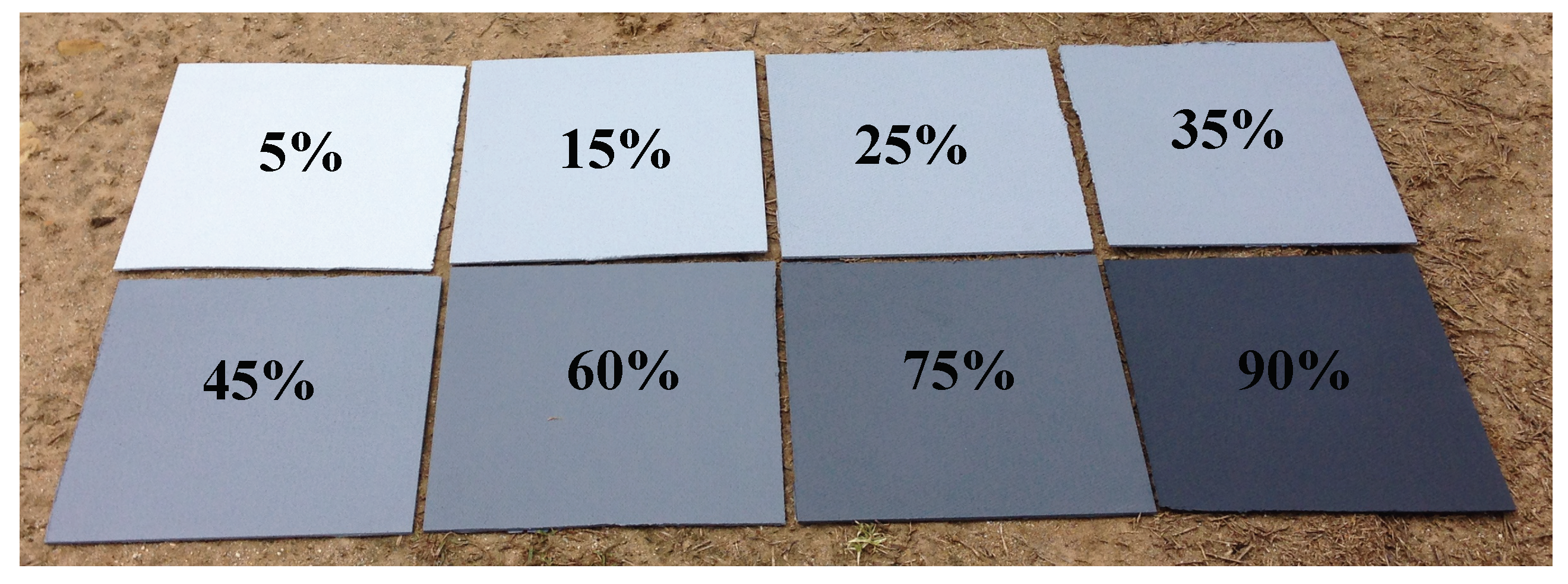
A grey calibration panel was built out of Masonite hardboard to establish the relationships between surface reflectance and image raw DN. Eight reference surfaces were painted using a grey gradient ranging from 5% to 90% (Figure 2). The percent grey values referred to the proportion of pure black paint mixed into pure white paint using dosing syringes. The paint was applied in two layers across the rough side of the board. The dimensions of each unit were: 30.5 cm × 30.5 cm ×0.3 cm.
Surface reflectance of the grey calibration panel was measured using an Ocean Optics Flame miniature spectrometer (Ocean Optics Inc., Largo, FL, USA) connected to a diffuse reflectance probe with built-in halogen source. The light was first emitted from the built-in halogen source onto a blank (Lambertian) surface to measure the intensity of the incoming light beam across its spectrum ranging from 400 nm in the visible to 1000 nm in the near-infrared. Light was then emitted onto each reference surface to measure the intensity of the reflected light beams across the [400–1000] nm spectrum. The reflectance in the four multispectral bands was calculated as:
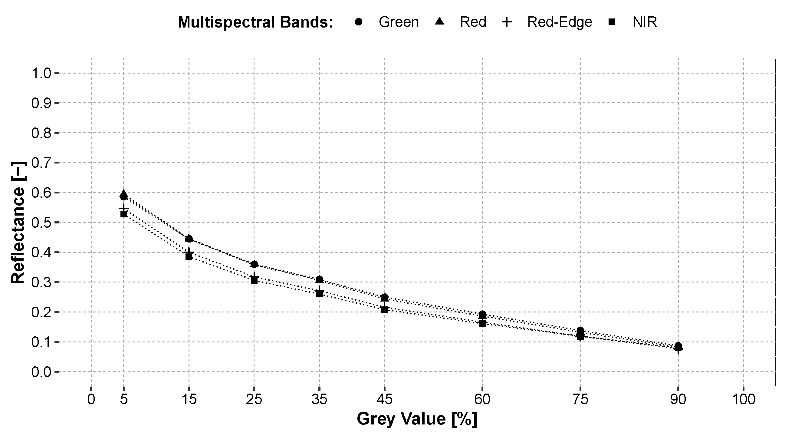
where is the incoming light intensity and is the reflected light intensity at wavelength , respectively, i is the lower, and j the upper limit of the wavelength band of interest. i and j were equal to 480 nm and 520 nm for the green band, 640 nm and 680 nm for the red band, 730 nm and 740 nm for the red-edge band, and 770 nm and 810 nm for the near-infrared band. Reflectance decreased exponentially as the percent grey value increased and the reflectance values measured for the different reference surfaces in each band (Figure 3).
2.5. Calibration Equations
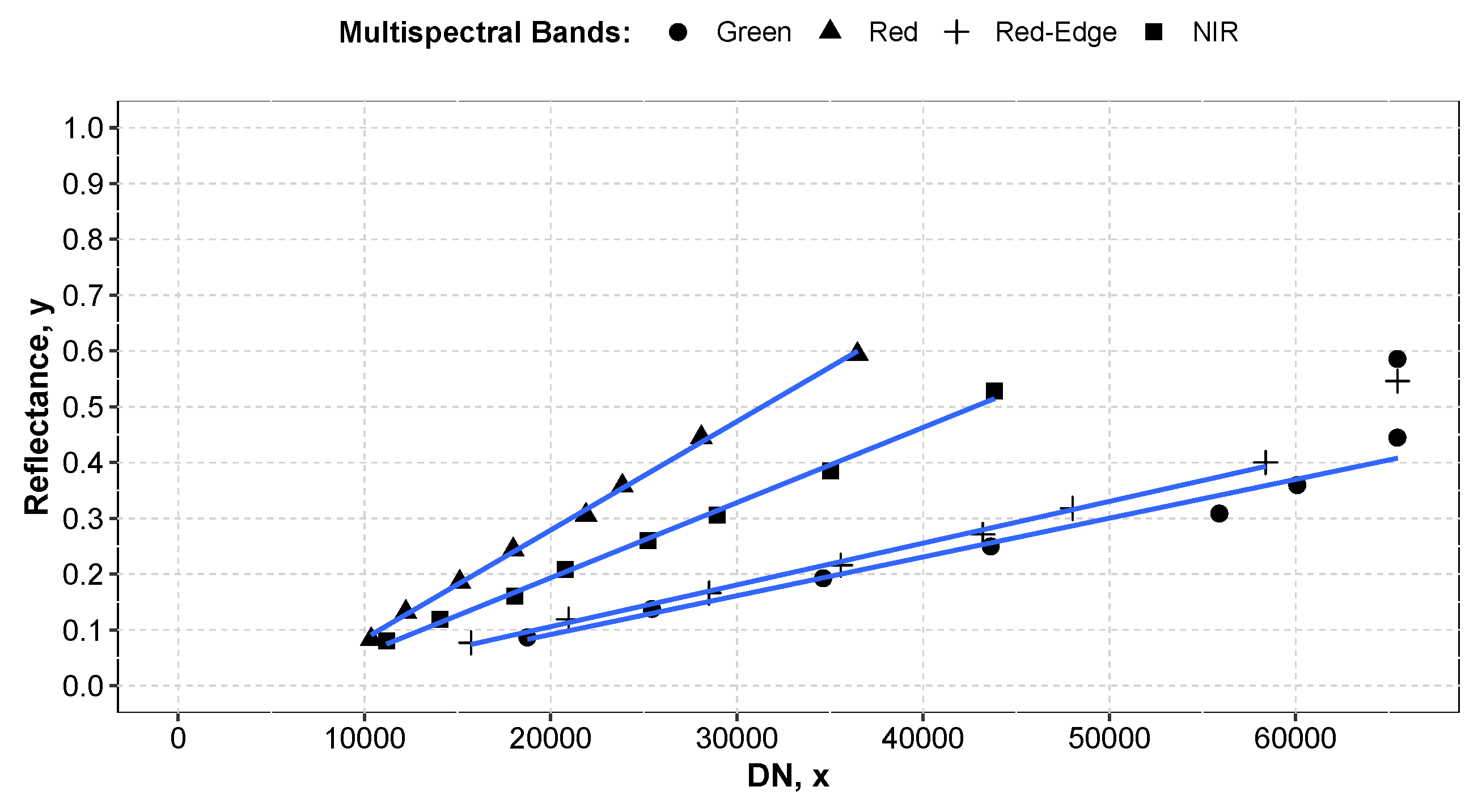
Pictures of the grey calibration panel (Figure 2) were taken at solar noon on a clear day with the Parrot Sequoia® camera at three different viewing angles. The 16-bit DNs were extracted from the pictures using R software [33] (Figure 4). Higher DN were associated with higher reflectance values and therefore, clearer surfaces. Linear relationships were established between raw DN and surface reflectance in each camera band (Figure 5 and Table 4). These relationships were used throughout this study to calibrate the data using methods C, D, and E. The r values reported in Table 4 indicate the amount of random noise within each band. Slightly higher noise was observed in the green and red-edge bands than in the red and NIR bands.
2.6. Data Collection
UAS data were collected across a 30 ha field planted with corn, cotton, and soybeans (Figure 6). Twenty-five calibration targets and five sets of three validation targets were built using the same material and paint mix than what was used to create the reference surfaces. The calibration targets were painted using the 25% grey value. The validation targets were painted using 5%, 25%, and 75% grey values. The targets’ dimensions were 61 cm × 122 cm. The reflectance of all targets was measured before and after data collection using the setup described in Section 2.4. Student t-tests were computed to compare target reflectance to the reflectance of the corresponding reference surfaces. Measured reflectance values before data collection were uniform between targets and not statistically different from the reflectance of the corresponding reference surfaces. Measured reflectance values between targets were more variable after data collection, but overall, the reflectance was still not statistically different from the reflectance of the corresponding reference surfaces. All targets were placed across the field before flights and removed after to limit weather exposure. The calibration targets were used to pre-calibrate the raw images with method C and to post-calibrate the processed rasters with methods D and E. The calibration targets were distributed across the field so that at least one target was within each raw image. The validation targets were used to evaluate the performance of all five calibration methods.
2.7. Raw Image Calibration with Method C
This section describes how the linear relationships presented in Figure 5 were used to calibrate the raw images using method C. True reflectance in all bands was defined as:
where is the true reflectance, is the reference raw digital number associated with , a is the slope, and b is the intercept. All parameters in Equation (2) are known. Wang and Myint (2015) [28] established that b is constant and only a changes for each image. Hence, measured reflectance of any pixel within the image is:
where is the pixel measured reflectance, is the pixel raw digital number, is the image specific slope, and b is the constant intercept. and b are known. and are unknown. For all pixels within a calibration target, measured reflectance should be equal to true reflectance:
where is the measured reflectance of the pixels within a calibration target, is the true reflectance of the pixels within a calibration target, is the measured raw digital number of the pixels within a calibration target, is the image specific slope, and b is the constant intercept. Using Equation (5) we calculated the image specific slope as:
where is the image specific slope, is the measured reflectance of the pixels within a calibration target, is the true reflectance of the pixels within a calibration target, is the measured raw digital number of the pixels within a calibration target, and b is the constant intercept. Then, substituting Equation (4) within Equation (3) we calculated the calibrated reflectance of all pixels within a raw image as:
where is the calibrated reflectance of all pixels within an image, is the true reflectance of the pixels within a calibration target, is the measured raw digital number of the pixels within a calibration target, is the raw digital numbers of all pixels within an image, and b is the constant intercept.
2.8. Data Analysis
2.8.1. Objective 1: Compare the Accuracy of the Different Radiometric Calibration Methods
Radiometric calibration method accuracy was considered as the ability to produce UAS imagery that accurately describes surface reflectance in all multispectral bands. The accuracy was evaluated using the five sets of validation targets placed throughout the experimental site. The root-mean-square error (RMSE) of the difference between validation target measurements and true reflectance values was used to quantify data accuracy. First, RMSE values were calculated across flights for each method, band, and grey value as:
where is the RMSE calculated across flights for method m, band b, and grey value s. , , and . is the total number of validation targets with grey value s found within all images produced for band b using calibration method m. . . is the measured reflectance of target i, is the true reflectance of target i. RMSE values were then calculated for each method and band across grey values and flights as:
where is the RMSE calculated across flights and grey values for method m and band b. The parameters methods A–E, and {green, red, red-edge, NIR}. is the total number of validation targets found within all images produced for band b using calibration method m. . . is the measured reflectance of target i, is the true reflectance of target i. Finally, RMSE values were calculated for each method across bands, grey values, and flights as:
where is the RMSE calculated for method m across bands, grey values, and flights. The parameter methods A–E. is the total number of validation targets found within all images produced using calibration method m. . . is the measured reflectance of target i, is the true reflectance of target i. Differences in data accuracy between multispectral bands for each calibration method were quantified by computing the coefficient of variation (CV) of the RMSE values calculated across flights and grey values in each band. These values were calculated as:
where is the coefficient of variation of the RMSE values calculated across flights and grey values for method m and band b. is the standard deviation of the calculated in the Green, Red, and Red-Edge channels for method m. is the mean of the four calculated in the Green, Red, and Red-Edge channels for method m.
2.8.2. Objective 2: Quantify the Radiometric Error Associated with Each Calibration Method
Measured reflectance of the validation targets for each grey value, multispectral band, and radiometric calibration method was calculated as:
where is the measured reflectance of the validation targets associated with method m, band b, and grey value s. is the total number of validation targets with grey value s found within all images produced for band b using calibration m. = 5 targets × 7 flights = 35 targets. . is the measured reflectance of target i.
Linear regressions were computed to model relationships between measured and true reflectance for each band and calibration method. The goodness of fit was evaluated based on the adjusted R values. Measured reflectance of the validation targets was estimated as:
where is the measured reflectance of the validation targets associated with method m, band b, and grey value s. is the true reflectance of the validation targets of grey value s. The parameters and are the slope and intercept values computed for method m and band b, respectively. The radiometric error was the difference between measured and true reflectance values and calculated as:
where is the radiometric error associated with method m and band b. is the true reflectance in band b. The parameters and are the slope and intercept values of the linear regressions correlating measured to true reflectance values.
The radiometric error was calculated across the collected imagery for each flight date, multispectral band, and calibration method. Data were summarized to show the cumulative distribution of error associated with each band and calibration method and the differences observed between flights.
2.8.3. Objective 3: Quantify the Accuracy of Vegetation Indices
Multispectral UAS imagery is used to calculate different indices known to correlate with biophysical processes. The radiometric error propagates in the calculated value, which can affect data accuracy. The normalized difference vegetation index (NDVI) and the normalized difference red-edge index (NDRE) are two widely used indices in agriculture, and both were used to investigate how the radiometric error affects data accuracy of vegetation indices. NDVI and NDRE can be calculated from the red, red-edge, and NIR bands. Their general equation is:
For the NDVI, z is the NDVI, x is NIR, and y is red. For the NDRE, z is the NDRE, x is NIR, and y is red-edge. The error propagation for the indices was calculated by partial derivation of Equation (14) with respect to x and y as described by [34]:
where is the error of the computed vegetation index, and and are the errors of the corresponding bands.
NDVI and NDRE maps were computed, and the radiometric error across the study area was calculated for each flight date and radiometric calibration method. Data were summarized to show the cumulative distribution of error associated with each index and calibration method as well as the differences observed between flights. Uncertainty was calculated as:
where , z, and , are the uncertainty, value, and error of the computed vegetation index. Boxplots were computed to show the distribution of uncertainty among the data as a function of NDRE and NDVI values.
3. Results
3.1. Objective 1: Compare the Performance of the Different Radiometric Calibration Methods
No radiometric calibration method minimized error for all grey values and multispectral bands (Table 5). On average, method D minimized error across bands and grey values closely followed by method E. Method D resulted in better data accuracy than method B, and results indicated that data quality provided by the manufacturer-recommended calibration could be further improved with an empirical calibration. Method E resulted in better data accuracy than method C, and results showed that calibrating the processed uncalibrated rasters would be preferable to calibrating the raw images before data processing. Method A provided lower data accuracy than the other four methods in the green, red, and red-edge bands. Method A failed to calibrate acquired imagery in the NIR band.
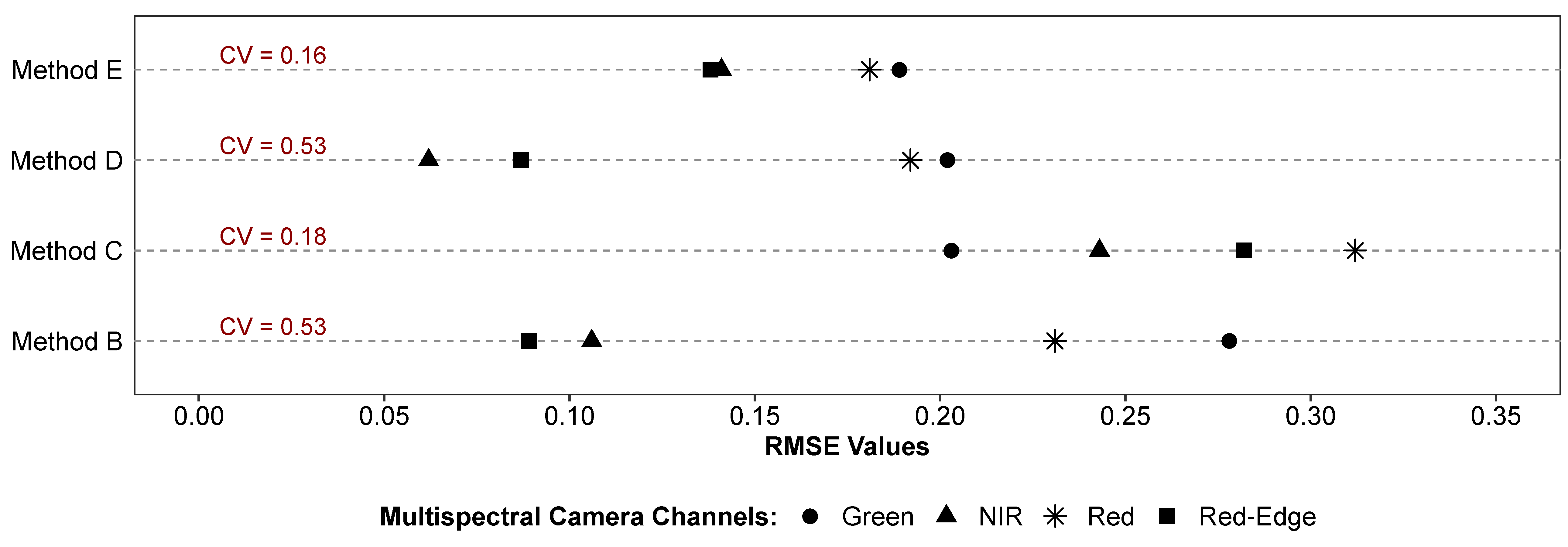
Data accuracy varied between the multispectral bands (Figure 7). For methods B and E, pixel reflectance values were more accurate in the red-edge and NIR band than in the green and red bands. For method D, pixel reflectance values were more accurate in the NIR and red-edge bands than in the green and red bands. Maximum differences between bands were observed for methods B and D. Minimum differences were observed for method E, closely followed by method C. These results showed that calibrating the data using the manufacturer-recommended method with or without empirical calibration increased accuracy variability between the different bands in comparison to the empirical calibration alone. Hence, even if method D was overall slightly more accurate than method E, using the latter would be preferable as its global RMSE value was very low, and differences in accuracy between multispectral bands were minimal.
Finally, data accuracy varied between the different grey values selected to build the validation targets (Table 5). For method E, pixel radiometric values were more accurate for the 25% grey value and least accurate for the 5% grey values in the green, red-edge, and NIR bands. No differences were observed between grey values in the red band. For methods D and C, pixel radiometric values were more accurate for the 25% grey value in all four bands, least accurate for the 5% grey value in the green and red bands, and least accurate for the 75% grey value in the red-edge and NIR bands. For method B, there were some differences between grey values in each band, but these differences were not structured as for the other methods. Calibration of the data with any of the empirical methods resulted in higher accuracy for the reflectance values nearing the reflectance of the targets used for calibration.
3.2. Objective 2. Quantify the Radiometric Error Associated with Each Calibration Method
Measured reflectance was linearly correlated to true reflectance for each multispectral band and radiometric calibration method (Figure 8). All radiometric calibration methods overestimated low reflectance values while underestimating high reflectance values. Linear coefficients describing the relationship between measured and true reflectance values varied between the different bands and methods. Higher slopes indicated stronger relationships between measured and true reflectance and therefore, higher data accuracy. Method C provided poor results in all bands. Accuracy of methods B, D, and E varied between bands. The strongest correlations were observed in the red-edge and NIR bands for method B and D, and in the red band for method E. These results demonstrated that radiometric error varied with pixel radiometric value. As measured reflectance was linearly correlated to true reflectance, then the radiometric error was also linearly correlated to pixel radiometric value (Table 6). Linear model goodness of fit was high in the green and red bands and very good in the red-edge and NIR bands.
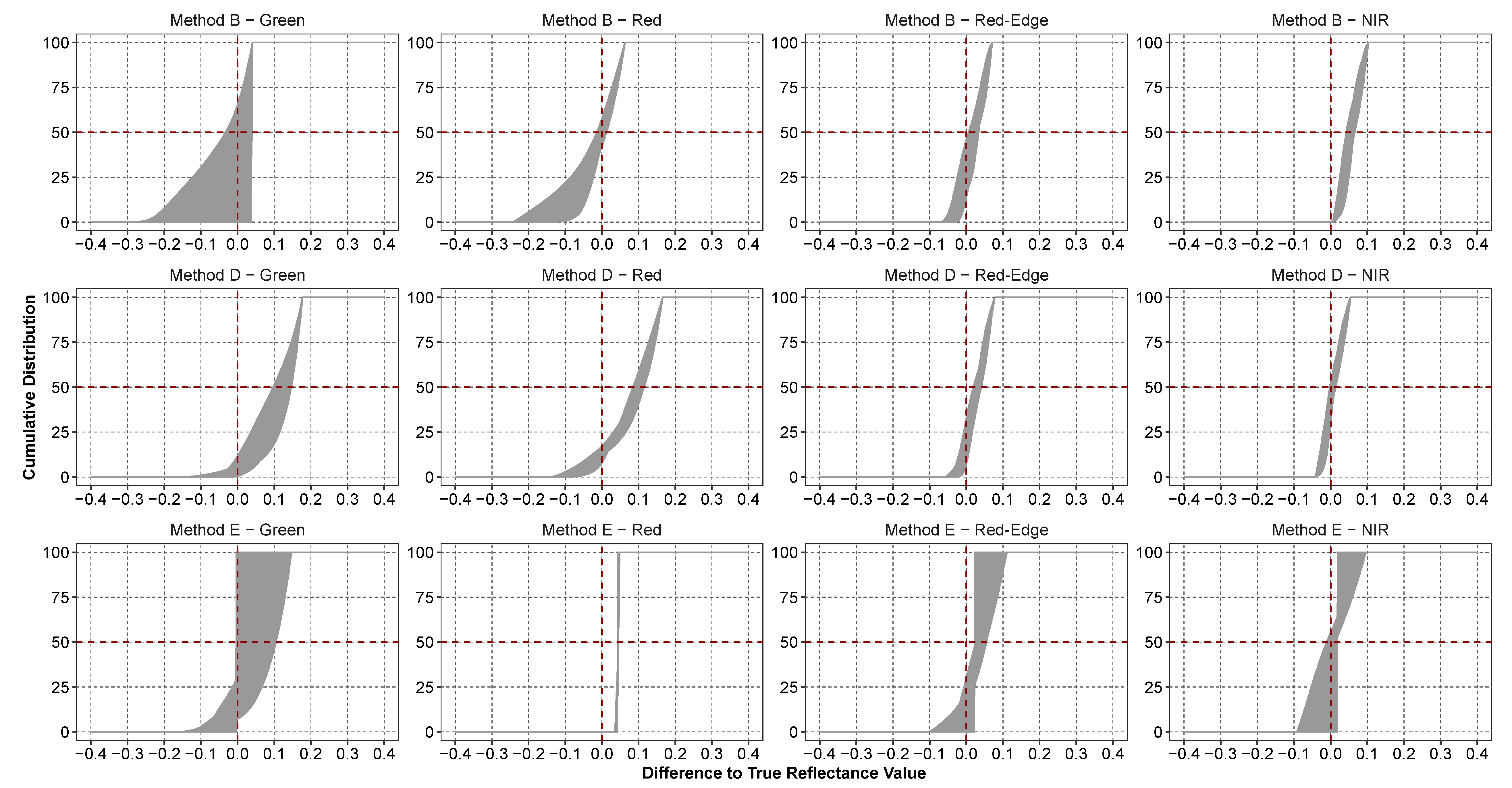
Overall, most pixel values were outside the validation range within the green and red bands, while most pixel values were within the validation range in the red-edge and NIR bands (Table 7). The radiometric error was calculated only for the pixels within the validation range, and the results presented in Figure 9 are representative of the percentages of pixels provided in Table 7. Radiometric error varied between multispectral bands and radiometric calibration methods (Figure 9). For method B, radiometric error ranged approximately from −0.30 to 0.05, −0.25 to 0.05, −0.08 to 0.08, and 0.00 to 0.10 in the green, red, red-edge, and NIR bands, respectively. For method D, radiometric error ranged approximately from −0.15 to 0.18, −0.15 to 0.15, −0.08 to 0.08, and 0.05 to 0.05 in the green, red, red-edge, and NIR bands, respectively. For method E, radiometric error ranged approximately from −0.18 to 0.12, 0.02 to 0.05, −0.10 to 0.10, −0.10 to 0.10 in the green, red, red-edge, and NIR bands, respectively. Furthermore, the distribution of radiometric error changed from flight to flight, and the magnitude of the differences observed between flights varied between multispectral bands and radiometric calibration methods. Radiometric error and radiometric error variability were both higher in the green band in comparison to the red, red-edge, and NIR bands, indicating lower data accuracy in this band, Finally, results demonstrated the existence of some bias in radiometric error distribution between multispectral bands for the different radiometric calibration methods. For instance, radiometric error distribution was biased toward negative values in the green channel for method B, and this method tended to underestimate reflectance values in the green band. On the other hand, radiometric error distribution was biased toward positive values in the NIR band for method B, and in the red band for method D. Therefore, methods B and D tended to overestimate reflectance values in the NIR and red bands, respectively.
3.3. Objective 3: Quantify the Accuracy of Vegetation Indices
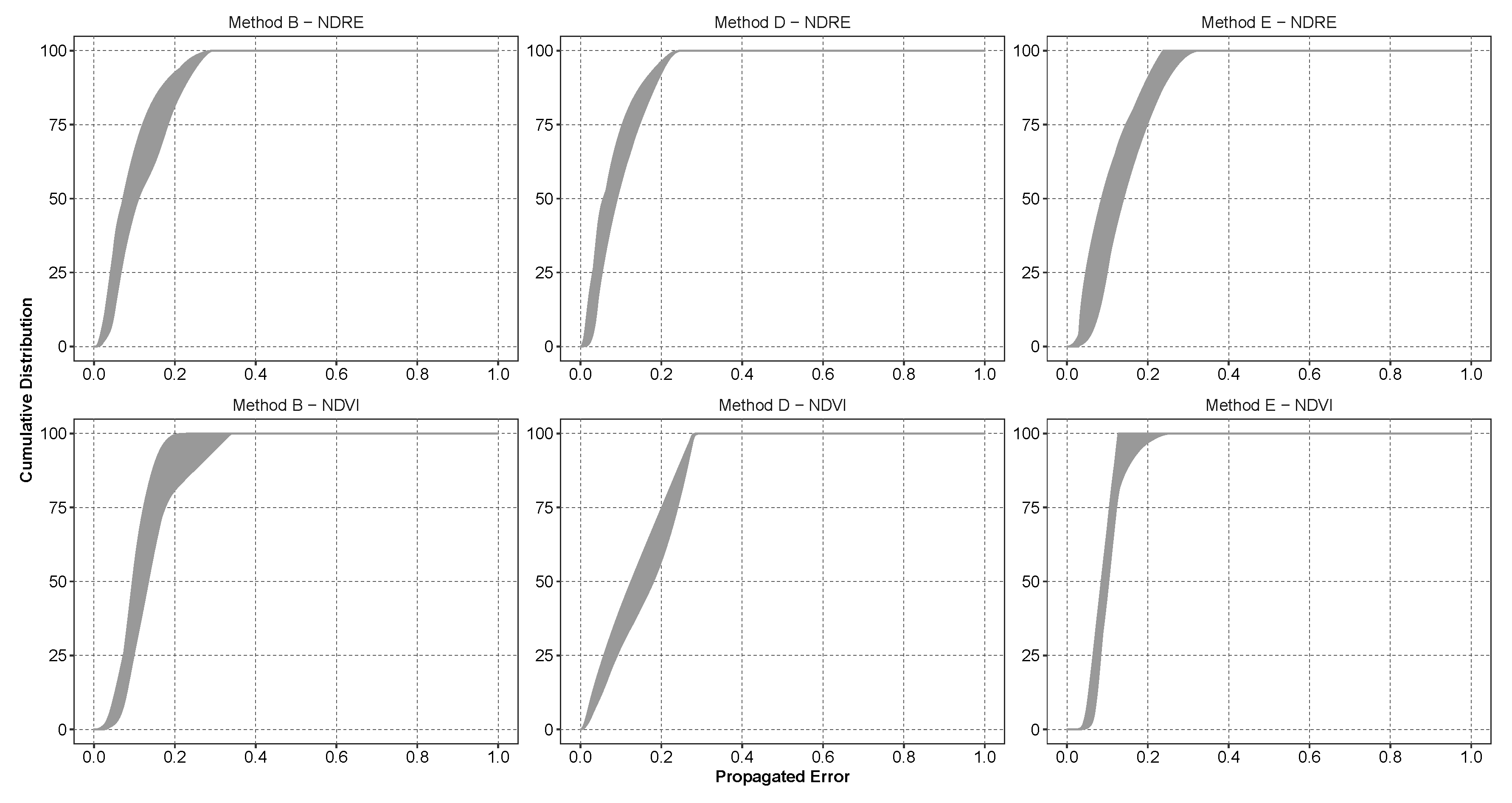
Error propagation for the NDVI and NDRE data was calculated using only the red, red-edge, and NIR pixels found to be within the validation range. The propagated error of indices and radiometric calibration methods was similar (Figure 10). For all methods and indices, the propagated error ranged from 0.00 to 0.25. More than 50% of the error ranged from 0.00 to 0.10. Little variability was observed between flights.
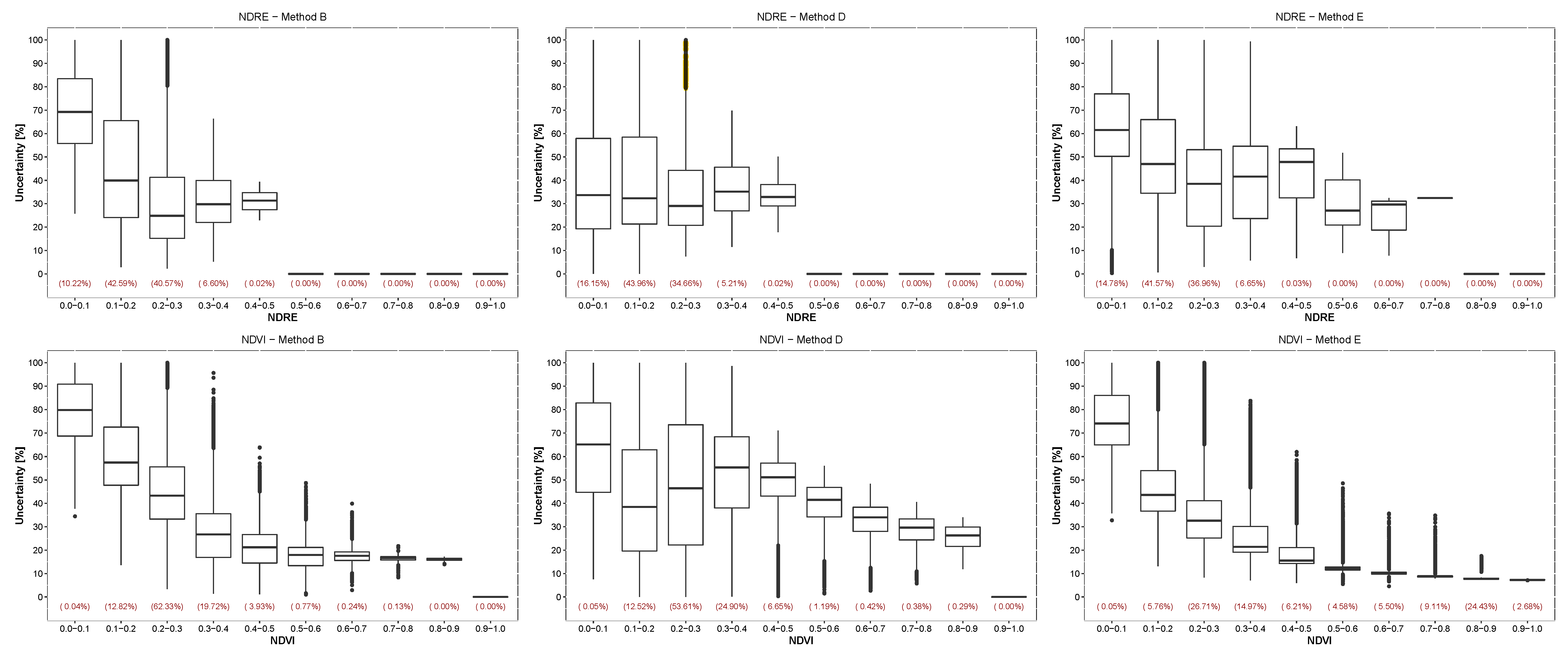
Uncertainty within the NDRE and NDVI data varied across index values (Figure 11). Uncertainty reduced with increasing NDRE and NDVI values. For instance, uncertainty obtained using method B reduced from 70% to 30% when NDRE values increase from 0.0–0.1 to 0.4–0.5, and from 80% to 15% when NDVI values increased from 0.0–0.1 to 0.8–0.9. Error variability also tended to reduce with increasing NDRE and NDVI values. For instance, with method D, NDRE values of 0.0–0.1 were associated with an uncertainty ranging from 20% (first quarter) to 60% (last quarter) when NDRE values of 0.4–0.5 were associated with uncertainties ranging from 30% to 40%. Overall, slightly higher data accuracy was achieved with method D for the NDRE data, and with method E for the NDVI data. Error variability achieved with methods B and D was smaller for NDVI in comparison to NDRE.
4. Discussion
None of the radiometric calibration methods minimized the error in all multispectral bands. Data accuracy achieved with the manufacturer-recommended method was comparable to the accuracy achieved with the empirical methods tested in this study. However, the manufacturer method resulted in bigger differences in accuracy between multispectral bands than the empirical methods. Lower accuracy was achieved in the green and red bands, possibly due to increased Rayleigh scattering in lower wavelength bands. The manufacturer-recommended method might perform poorer in the green and red bands because it does not correct for the atmospheric radiance effects in comparison to the empirical methods. The combination of the manufacturer method with an empirical calibration further improved data accuracy in all bands but did not reduce the magnitude of the differences between bands. The manufacturer methods are typically easier and quicker to implement than the empirical methods, and they do not require additional labor or expert knowledge to generate calibrated imagery. Our results show that these methods could constitute a suitable alternative to empirical methods to provide growers with calibrated UAS imagery. Further research should be conducted to evaluate the performance of other manufacturer methods developed with other cameras.
For the empirical methods, Wang and Myint [28] recommended placing enough calibration targets across the study area to have at least one target within each raw image, so that the raw images can be calibrated before data processing. Higher data accuracy was achieved when the simplified empirical line method was applied to the processed rasters rather than the raw images, and implementation of this method could be simplified by reducing the number of calibration targets placed across the study area. Further research should be conducted to determine the optimum calibration target resolution required to maximize data accuracy while limiting resources requirements to implement this method.
For the empirical methods, the radiometric error was smaller for surface reflectance closer to the reflectance of the calibration targets. Such results indicated that data accuracy achieved with the simplified empirical line method could be further improved using more than one grey value to calibrate the processed rasters. The authors would recommend using at least three grey values with low, medium, and high surface reflectance to account for possible non-linear relationships between radiometric error and surface reflectance.
Proper calibration of UAS data can only be achieved within the range of reflectance represented by the grey gradient calibration panel as the calibration equations should not be applied outside of the calibration range. The calibration panel used in this study could be used to calibrate most but not all pixels within the collected imagery. Hence, the authors would recommend adding white and black reference surfaces to the calibration panel to account for a broader range of surface reflectance within the collected imagery. These would correspond to grey values of 0% and 100%, respectively.
In our results, the relationships between surface reflectance and raw DN in all multispectral bands were linear. These relationships were exponential in Wang and Myint’s [28] study. These differences are explained by the fact that different cameras were used in the two studies. There was saturation in the green and red-edge bands. The saturation of the green band (Figure 5) explains the poor data accuracy of this band throughout the study independently from the calibration methods. Increased Rayleigh scattering in the green band in comparison to the red, red-edge, and NIR bands could have contributed to saturating the green sensor. However, based on Chiliński and Ostrowski’s results [14], the authors don’t think this effect was significant. In Figure 5 we showed that saturation in the green band was observed for reflectance values larger than 0.35. This means that about 64% of the possible reflectance in this band results in the same DN value. The Parrot Sequoia camera sets the same exposure time for all four bands, while exposure time for the green channel should be shorter to avoid saturation of the sensor. DN saturation was also discussed by Wang and Myint [28] and should be recognized when analyzing the data or composing it into new indices. Further research could also be conducted to include empirical methods or radiative transfer model for haze estimation and correction in the particular case of low altitude UAS imagery.
Uncertainty of NDVI and NDRE indices decreased with increasing index values (Figure 11). Error variability also decreased with increasing index values. Defries and Townshend [35] reported NDVI values of 0.1 for bare ground and 0.0–0.6 for cultivated land on the northern hemisphere. For forests, Defries and Townshend [35] reported NDVI values of , 0.0–0.6, and −0.2–0.6 for broadleaf evergreen, broadleaf deciduous, and coniferous evergreen, respectively. Teal et al. [36] measured NDVI values between 0.3 and 0.9 for corn (Zea mays). Depending on land use, NDVI uncertainty could be fairly low or significantly high.
Behmann et al. [37] stressed barley (Hordeum vulgare) by reducing irrigation water. Stressed plants and well-watered plants had NDVI values of 0.45–0.75 and the median uncertainty for this NDVI range is 10–20% (Figure 11). Although these uncertainty values are relatively small in comparison to lower NDVI index values, in the case of Behmann et al.’s [37] experiments, water stress would not have been detected at all or not until 30 days after water stress induction.
Li et al. [38] measured NDRE values in corn (Zea mays) of 0.2–0.6, which corresponds to an uncertainty range of 30–50% (Figure 11). Higher NDVI and NDRE values characterize denser canopy covers, and results indicated that data quality achieved with the different radiometric calibration methods was overall higher for dense vegetative covers in comparison to lighter covers or bare soil. Our results showed that different methods resulted in different data accuracy for each range of NDRE and NDVI value. Therefore, the radiometric calibration method should be selected according to the vegetative index of interest and the range of index values expected to be observed within the imagery.
Finally, one should keep in mind that this study was conducted using one camera, and different results might be obtained with other cameras due to the use of different bands or lenses of different quality. Different camera systems might be characterized by different noises associated with data collection. Instrumental random noise was not accounted for in this study because data were collected using only one camera system. However, the authors recommend accounting for it when comparing the performance of different camera systems. Knowing the radiometric accuracy of collected imagery is critical to ensure the accuracy of subsequent analyses, and the authors recommend using surfaces of known reflectance to validate the data calibration and estimate radiometric error within every processed raster. The proper estimation of the error can only be achieved within the range of reflectance represented by the validation panel. The range of reflectance selected in this study was not wide enough to calculate radiometric error throughout the collected imagery. The authors recommend using surfaces of at least three different reflectance values—low, medium, and high —to be able to identify non-linear relationships between radiometric error and surface reflectance, if applicable.
5. Conclusions
No calibration method minimized radiometric error in all multispectral bands. Data accuracy achieved with the manufacturer-recommended method was comparable to the accuracy achieved with the empirical methods tested in this study. Better data accuracy was achieved when the simplified empirical line method was applied onto the processed raster rather than the raw images. The combination of the manufacturer method with an empirical calibration further improved data accuracy achieved with the manufacturer method in all multispectral bands. The radiometric error was not constant within an image but varied linearly with surface reflectance. All calibration methods overestimated low reflectance values while underestimating high reflectance values. Digital number saturation was an issue in the green band. Accuracy of the composite indices was higher for the pixels representing a dense vegetative cover in comparison to a lighter cover or bare soil. Depending on land use and vegetation index measurement uncertainty can be significantly higher. These results demonstrated that calibrating UAS imagery is not a straightforward process, and researchers must plan to evaluate the performance of their radiometric calibration before analyzing UAS imagery and interpreting the results.
Author Contributions
Conceptualization, A.M.P., T.K., C.B., J.N.S., M.F.J., and B.V.O.; methodology, A.M.P., T.K., and C.B.; software, A.M.P.; validation, A.M.P. and C.B.; formal analysis, A.M.P. and T.K.; investigation, A.M.P., T.K, and C.B.; resources, M.F.J. and T.K.; writing—original draft preparation, A.M.P. and T.K.; writing—review and editing, A.M.P., T.K., and M.F.J.; visualization, A.M.P. and T.K.; supervision, T.K.; project administration, T.K.; funding acquisition, T.K., J.N.S., and B.V.O.
Funding
This project was supported by the Alabama Farmers Federation, the Alabama Agricultural Experiment Station, and the Hatch program of the National Institute of Food and Agriculture, U.S. Department of Agriculture.
Conflicts of Interest
There are no conflict of interest.
References
- USGS. Landsat Missions—What Are the Acquisition Schedules for the Landsat Satellites; USGS: Reston, VA, USA, 2017.
- USGS. Landsat Missions—What Are the Band Designations for the Landsat Satellites; USGS: Reston, VA, USA, 2017.
- Mainy, A.; Agrawal, V. Satellite Technology: Principles and Applications; John Wiley & Sons: Hoboken, NJ, USA, 2011. [Google Scholar]
- Remondino, F.; Barazzetti, L.; Nex, F.; Scaioni, M.; Sarazzi, D. UAV Photogrammetry for Mapping and 3D Modeling—Current Status and Future Perspectives. Int. Arch. Photogramm. Remote Sens. Spat. Inf. Sci. 2011, 38, C22. [Google Scholar] [CrossRef]
- Zhang, C.; Kovacs, J. The Application of Small Unmanned Aerial Systems for Precision Agriculture: A Review. Precis. Agric. 2012, 13, 693–712. [Google Scholar] [CrossRef]
- Laliberte, A.; Goforth, M.; Steele, C.; Rango, A. Multispectral Remote Sensing from Unmanned Aircraft: Image Processing Workflows and Applications for Rangeland Environments. Remote Sens. 2011, 3, 2529–2551. [Google Scholar] [CrossRef] [Green Version]
- Hruska, R.; Mitchell, J.; Anderson, M.; Glenn, N. Radiometric and Geometric Analysis of Hyperspectral Imagery Acquired from an Unmanned Aerial Vehicle. Remote Sens. 2012, 4, 2736–2752. [Google Scholar] [CrossRef] [Green Version]
- Gauci, A.; Brodbeck, C.; Poncet, A.; Knappenberger, T. Assessing the Geospatial Accuracy of Aerial Imagery Collected with Various UAS Platforms. Trans. ASABE 2018, 61, 1823–1829. [Google Scholar] [CrossRef]
- Jones, H.; Vaughan, R. Chapter 621, Preparation and Manipulation of Optical Data, Image Correction, Geometric Correction. In Remote Sensing of Vegetation: Principles, Techniques, and Applications; Oxford University Press: Oxford, UK, 2010. [Google Scholar]
- Jones, H.; Vaughan, R. Chapter 622, Preparation and Manipulation of Optical Data, Image Correction, Radiometric Correction. In Remote Sensing of Vegetation: Principles, Techniques, and Applications; Oxford University Press: Oxford, UK, 2010. [Google Scholar]
- Richter, R. Correction of Atmospheric and Topographic Effects for High Spatial Resolution Satelite Imagery. Remote Sens. 1997, 18, 1099–1111. [Google Scholar] [CrossRef]
- Bucholtz, A. Rayleigh Scattering Calculations for the Terrestrial Atmosphere. Appl. Opt. 1995, 34, 2765–2773. [Google Scholar] [CrossRef]
- Kedzierski, M.; Wierzbicki, D.; Sekrecka, A.; Fryskowska, A.; Walczykowski, P.; Siewert, J. Influence of Lower Atmosphere on the Radiometric Quality of Unmanned Aerial Vehicle Imagery. Remote Sens. 2019, 11, 1214. [Google Scholar] [CrossRef]
- Chiliński, M.; Ostrowski, M. Error Simulations of Uncorrected NDVI and DCVI during Remote Sensing Measurements from UAS. Misc. Geogr. 2014, 18, 35–45. [Google Scholar] [CrossRef]
- Iqbal, F.; Lucieer, A.; Barry, K. Simplified Radiometric Calibration for UAS-Mounted Multispectral Sensor. Eur. J. Remote Sens. 2018, 51, 301–313. [Google Scholar] [CrossRef]
- Herrero-Huerta, M.; Hernández-López, D.; Rodriguez-Gonzalvez, P.; González-Aguilera, D.; González-Piqueras, J. Vicarious Radiometric Calibration of a Multispectral Sensor from an Aerial Trike Applied to Precision Agriculture. Comput. Electron. Agric. 2014, 108, 28–38. [Google Scholar] [CrossRef]
- Del Pozo, S.; Rodríguez-Gonzálvez, P.; Hernández-López, D.; Felipe-García, B. Vicarious Radiometric Calibration of a Multispectral Camera on Board of an Unmanned Aerial System. Remote Sens. 2014, 6, 1918–1937. [Google Scholar] [CrossRef]
- Karpouzli, E.; Malthus, T. The Empirical Line Method for the Atmospheric Correction of IKONOS Imagery. Int. J. Remote Sens. 2003, 24, 1143–1150. [Google Scholar] [CrossRef]
- Gao, B.C.; Montes, M.; Davis, C.O.; Goetz, A. Atmospheric Correction Algorithms for Hyperspectral Remote Sensing Data of Land and Ocean. Remote Sens. Environ. 2009, 113, S17–S24. [Google Scholar] [CrossRef]
- Kutser, T.; Pierson, D.; Kallio, K.; Reinart, A.; Sobek, S. Mapping Lake CDOM by Satellite Remote Sensing. Remote Sens. Environ. 2005, 94, 535–540. [Google Scholar] [CrossRef]
- Jakob, S.; Zimmermann, R.; Gloaguen, R. The Need for Accurate Geometric and Radiometric Corrections of Drone-Borne Hyperspectral Data for Mineral Exploration: MEPHySTo—A Toolbox for Pre-Processing Drone-Born Hyperspectral Data. Remote Sens. 2017, 9, 88. [Google Scholar] [CrossRef]
- Smith, G.; Milton, E. The Use of the Empirical Line Method to Calibrate Remotely Sensed Data to Reflectance. Int. J. Remote Sens. 1999, 20, 2653–2662. [Google Scholar] [CrossRef]
- Von Bueren, S.; Burkard, A.; Hueni, A.; Rascher, U.; Tuohy, M.; Yule, I. Deploying Four Optical UAV-Based Sensors over Grassland: Challenges and Limitations. Biogeosciences 2015, 12, 163–175. [Google Scholar] [CrossRef]
- Baugh, W.; Groeneveld, D. Empirical Proof of the Empirical Line. Int. J. Remote Sens. 2008, 29, 665–672. [Google Scholar] [CrossRef]
- Stow, D.; Hope, A.; Nguyen, T.; Phinn, S.; Benkelman, C. Monitoring Detailed Land Surface Changes Using an Airborne Multispectral Digital Camera System. Trans. Geosci. Remote Sens. 1996, 34, 1191–1203. [Google Scholar] [CrossRef]
- Farrand, W.; Singer, R.; Merényu, E. Retrieval of Apparent Surface Reflectance from AVIRIS Data: A Comparison of Empirical Line, Radiative Transfer, and Spectral Mixture Methods. Remote Sens. Environ. 1994, 47, 311–321. [Google Scholar] [CrossRef]
- Price, R.; Anger, C.; Mah, S. Preliminary Evaluation of casi Preprocessing Techniques. In Proceedings of the 17th Canadian Symposium on Remote Sensing, Saskatoon, SK, Canada, 13–15 June 1995; pp. 694–697. [Google Scholar]
- Wang, C.; Myint, S. A Simplified Empirical Line Method of Radiometric Calibration for Small Unmanned Aircraft Systems-Based Remote Sensing. IEEE J. Sel. Top. Appl. Earth Obs. Remote Sens. 2015, 8, 1876–1885. [Google Scholar] [CrossRef]
- Tu, Y.; Phinn, S.; Johansen, K.; Robson, A. Assessing Radiometric Correction Approaches for Multi-Spectral UAS Imagery for Horticultural Applications. Remote Sens. 2018, 10, 1684. [Google Scholar] [CrossRef]
- Singh, K.; Frazier, A.E. A Meta-Analysis and Review of Unmanned Aircraft System (UAS) Imagery for Terrestrial Applications. Int. J. Remote Sens. 2018, 39, 5078–5098. [Google Scholar] [CrossRef]
- SenseFly. EBee Plus Drone User Manual; SenseFly Inc.: Cheseaux-sur-Lausanne, Switzerland, 2019. [Google Scholar]
- MicaSense. Parrot Sequoia® Datasheet: The Multi-Band Sensor Designed for Agriculture; MicaSense, Inc.: Seattle, WA, USA, 2019. [Google Scholar]
- R Core Team. R: A Language and Environment for Statistical Computing; R Foundation for Statistical Computing: Vienna, Austria, 2019. [Google Scholar]
- Taylor, J. Introduction to Error Analysis, the Study of Uncertainties in Physical Measurements, 2nd ed.; University Science Books: New York, NY, USA, 1997. [Google Scholar]
- Defries, R.S.; Townshend, J.R.G. NDVI-derived land cover classifications at a global scale. Int. J. Remote Sens. 1994, 15, 3567–3586. [Google Scholar] [CrossRef]
- Teal, R.; Tubana, B.; Girma, K.; Freeman, K.; Arnall, D.; Walsh, O.; Raun, W. In-season prediction of corn grain yield potential using normalized difference vegetation index. Agron. J. 2006, 98, 1488–1494. [Google Scholar] [CrossRef]
- Behmann, J.; Steinrücken, J.; Plümer, L. Detection of early plant stress responses in hyperspectral images. ISPRS J.Photogramm. Remote Sens. 2014, 93, 98–111. [Google Scholar] [CrossRef]
- Li, F.; Miao, Y.; Feng, G.; Yuan, F.; Yue, S.; Gao, X.; Liu, Y.; Liu, B.; Ustin, S.L.; Chen, X. Improving estimation of summer maize nitrogen status with red edge-based spectral vegetation indices. Field Crops Res. 2014, 157, 111–123. [Google Scholar] [CrossRef]
Figure 1.
(a) Target used for the one-point calibration, one-point calibration plus sunshine sensor, and one-point calibration plus sunshine sensor plus post-calibration radiometric calibration methods. Target true reflectance was 17.9% in the green, 21.3% in the red, 26.3% in the red-edge, and 36.1% in the near-infrared. (b) Method used to take pictures of the calibration target at the time of flight.

Figure 2.
Grey calibration panel built to associate surface reflectance values with image raw digital numbers. The panel consisted of eight reference surfaces painted with a grey gradient ranging from 5% to 90%.
Figure 2.
Grey calibration panel built to associate surface reflectance values with image raw digital numbers. The panel consisted of eight reference surfaces painted with a grey gradient ranging from 5% to 90%.

Figure 3.
Surface reflectance of the grey gradient calibration panel measured in the different multispectral bands.
Figure 3.
Surface reflectance of the grey gradient calibration panel measured in the different multispectral bands.

Figure 4.
Example of an image used to determine surface reflectance raw DN associated with each grey value. Reference surfaces were delimited and pixel values were extracted using R. Raw DN for one reference surface in one image were calculated as the mean value of corresponding pixels. The standard deviation of all pixel values within one reference surface in one image was negligible in comparison to the mean. The standard deviation of the mean raw DN values for one reference surfaces between images was also negligible in comparison to the mean.

Figure 5.
Linear relationships between image raw digital numbers (DN) and surface reflectance in each multispectral band. The green and red-edge band sensors were saturated for the 5% reference surface and therefore that measurement was excluded from fitting linear equations.
Figure 5.
Linear relationships between image raw digital numbers (DN) and surface reflectance in each multispectral band. The green and red-edge band sensors were saturated for the 5% reference surface and therefore that measurement was excluded from fitting linear equations.

Figure 6.
(a) Picture of a calibration target used in this study for the radiometric calibration of multispectral unmanned aircraft systems (UAS) data using methods C, D, and E. (b) Picture of a set of validation targets used to evaluate the performance of all five calibration methods. Target dimensions were 61 cm × 122 cm. These dimensions were big enough for the target to be identified within the aerial images. It also allowed to select pixels values within the images not affected by the surrounding surfaces. (c) Calibration and validation target layout in the experimental field.
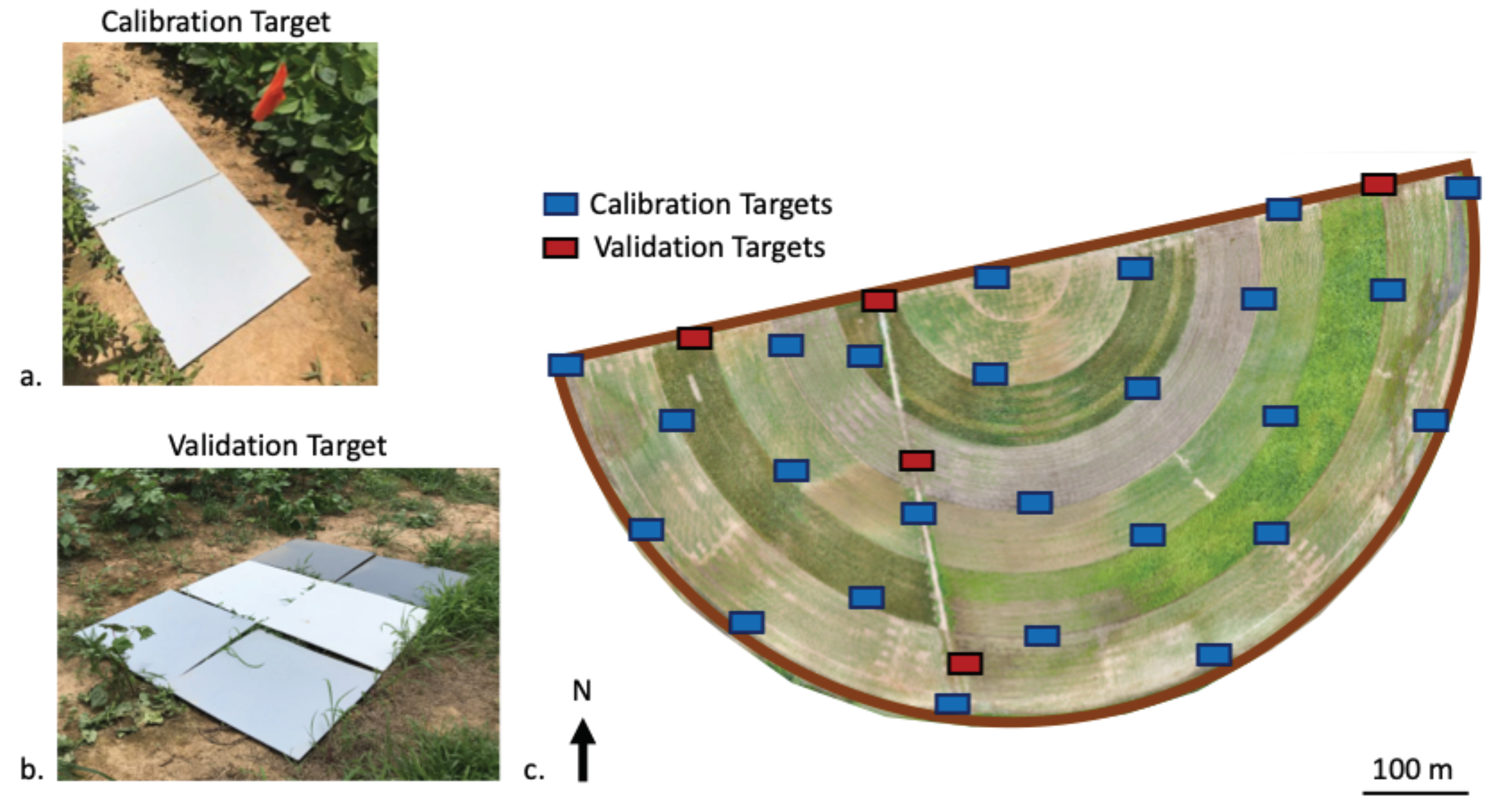
Figure 7.
Distribution of root-mean-square error (RMSE) values for each calibration method and multispectral band and associated coefficients of variation (CV).
Figure 7.
Distribution of root-mean-square error (RMSE) values for each calibration method and multispectral band and associated coefficients of variation (CV).

Figure 8.
Relationships between validation targets measured and true reflectance values for each multispectral band and radiometric calibration method. Measured reflectance values were calculated as the mean validation targets measured reflectance across flights. Confidence intervals around the measured reflectance values indicated the standard error of the mean measured reflectance between flights. Radiometric error corresponded to the difference between true and measured reflectance values and was represented in grey within individual plots.
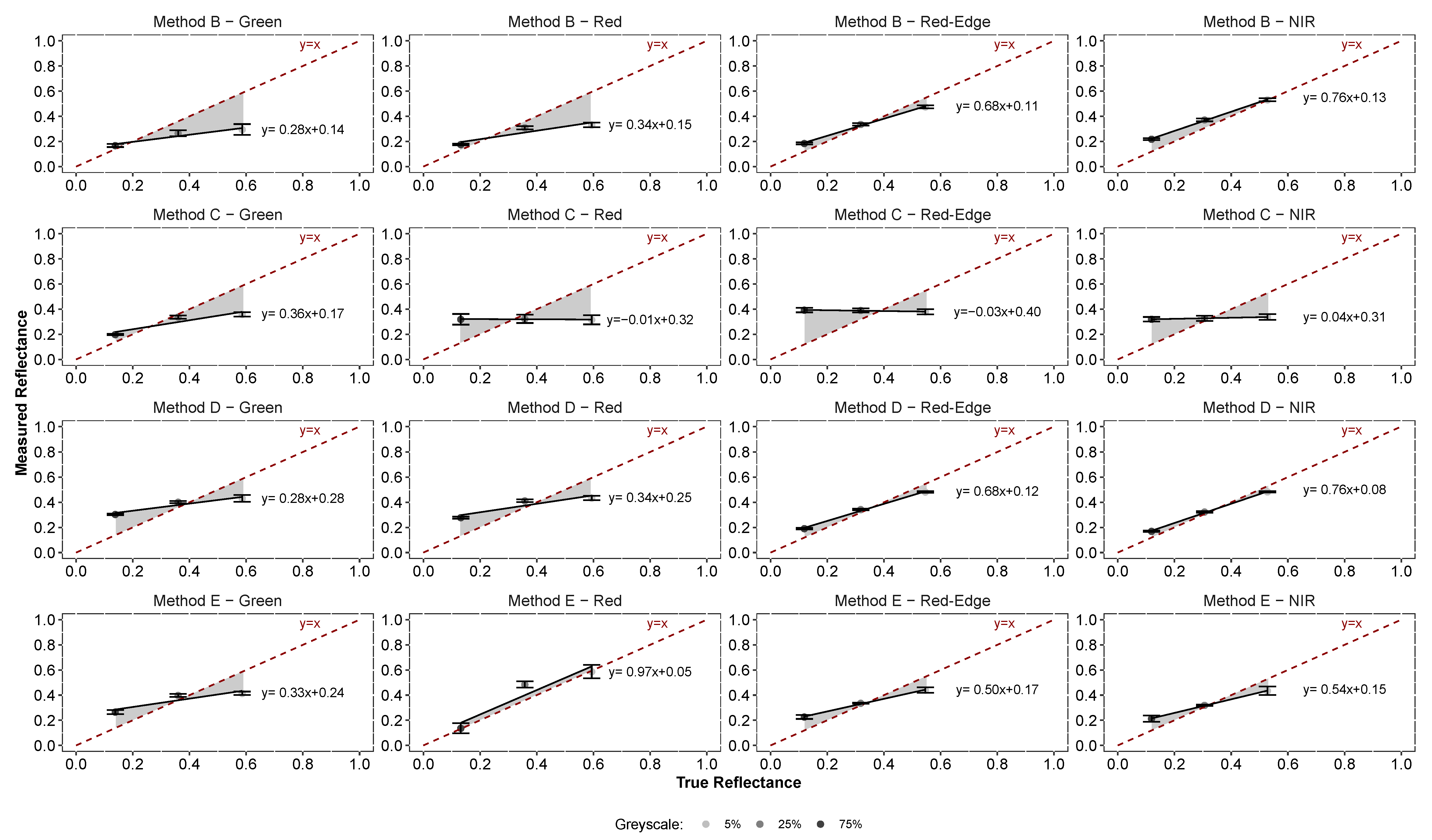
Figure 9.
Radiometric error cumulative distribution for each multispectral band and radiometric calibration method. The grey areas represent the variability observed between flights for each band and calibration method. The x = 0 and y = 50% lines were added to each plot to help identify radiometric error distribution bias.

Figure 10.
Cumulative distribution of the propagated error within the normalized difference vegetation index (NDVI) and normalized difference red-edge index (NDRE) data for radiometric calibration methods B, D, and E. The grey areas represent the variability observed between flights for index and calibration method.

Figure 11.
Uncertainty as a function of NDVI and NDRE values for radiometric calibration methods B, D, and E. The values in parentheses indicate the percentage of pixels within the image representative of the corresponding range of values on the x-axis.
Figure 11.
Uncertainty as a function of NDVI and NDRE values for radiometric calibration methods B, D, and E. The values in parentheses indicate the percentage of pixels within the image representative of the corresponding range of values on the x-axis.

Table 1.
Manufacturer technical specifications for the eBee Plus platform [31].
Table 1.
Manufacturer technical specifications for the eBee Plus platform [31].
| Aircraft | Horizontal Accuracy | ||
|---|---|---|---|
| Weight: | 1100 g | RTK Built-In: | Yes, activated |
| Size: | 110 cm | w/o GCP: | 3–5 cm |
| Wind Resistance: | 12 m/s | w/GCP: | 3–5 cm |
GCP: Ground Control Points.
Table 2.
Manufacturer technical specifications for the Parrot Sequoia multispectral camera [32].
Table 2.
Manufacturer technical specifications for the Parrot Sequoia multispectral camera [32].
| Camera | Band Definition | ||
|---|---|---|---|
| Weight: | 72 g | Green: | [480–520] nm |
| Dimensions: | 59 × 41 × 28 mm | Red: | [640–680] nm |
| Image Resolution: | 1280 × 960 pixels | Red-Edge: | [730–740] nm |
| HFOV/VFOV/DFOV: | 61.9o/48.5o/73.7o | NIR: | [770–810] nm |
HFOV: Horizontal Field of View;VFOV: Vertical Field of View; DFOV: Display Field of View; NIR: Near-Infrared.
Table 3.
Air temperature, humidity, wind speed, and cloud cover for each flight.
| Date | Start Time | End Time | Air Temperature | Humidity | Wind Speed | Cloud Cover |
|---|---|---|---|---|---|---|
| 19 July | 12:08 | 12:36 | 32.8 C | 66% | 0.0 m/s | Partly Cloudy |
| 2 August | 10:53 | 11:15 | 26.1 C | 75% | 2.6 m/s | Mostly Cloudy |
| 15 August | 12:04 | 12:40 | 31.1 C | 74% | 2.6 m/s | Partly Cloudy |
| 22 August | 10:45 | 11:09 | 31.1 C | 70% | 1.0 m/s | Clear |
| 29 August | 10:37 | 11:00 | 26.7 C | 68% | 1.5 m/s | Clear |
| 5 September | 11:27 | 11:51 | 29.4 C | 66% | 0.0 m/s | Clear |
| 19 September | 10:18 | 10:43 | 28.9 C | 73% | 0.0 m/s | Clear |
Table 4.
Linear equations describing the relationships between image raw digital numbers (DN) and surface reflectance in each multispectral band, and model goodness of fit as described by the adjusted R value.
Table 4.
Linear equations describing the relationships between image raw digital numbers (DN) and surface reflectance in each multispectral band, and model goodness of fit as described by the adjusted R value.
| Camera Band | Regression Equation | Goodness of Fit (r) |
|---|---|---|
| Green | 0.967 | |
| Red | 0.998 | |
| Red-Edge | 0.960 | |
| NIR | 0.996 |
Note: x represents the raw DNs and y represents surface reflectance.
Table 5.
Root-mean-square error (RMSE) values characterizing the performance of the different radiometric calibration methods across flights by multispectral band and grey value. RMSE values in the “all” columns were calculated across flights and grey values for each band, and across flights, grey values, and bands.
| Radiometric | Green | Red | Red-Edge | NIR | |||||||||||||
|---|---|---|---|---|---|---|---|---|---|---|---|---|---|---|---|---|---|
| Calibration | 5% | 25% | 75% | All | 5% | 25% | 75% | All | 5% | 25% | 75% | All | 5% | 25% | 75% | All | All |
| Method A | 0.310 | 0.241 | 0.187 | 0.364 | 0.267 | 0.293 | 0.210 | 0.376 | 0.485 | 0.375 | 0.235 | 0.549 | 16,383 | 12,169 | 8441 | 18,477 | 15,616 |
| Method B | 0.310 | 0.113 | 0.042 | 0.278 | 0.266 | 0.058 | 0.046 | 0.231 | 0.077 | 0.030 | 0.068 | 0.089 | 0.029 | 0.071 | 0.101 | 0.106 | 0.327 |
| Method C | 0.231 | 0.040 | 0.062 | 0.203 | 0.293 | 0.089 | 0.214 | 0.312 | 0.174 | 0.082 | 0.277 | 0.282 | 0.198 | 0.056 | 0.206 | 0.243 | 0.445 |
| Method D | 0.168 | 0.047 | 0.167 | 0.202 | 0.165 | 0.060 | 0.147 | 0.192 | 0.066 | 0.030 | 0.074 | 0.087 | 0.047 | 0.024 | 0.053 | 0.062 | 0.252 |
| Method E | 0.175 | 0.047 | 0.134 | 0.189 | 0.132 | 0.140 | 0.098 | 0.181 | 0.117 | 0.020 | 0.114 | 0.138 | 0.125 | 0.018 | 0.112 | 0.141 | 0.277 |
Table 6.
Linear relationships describing measured reflectance deviance to true reflectance values for each multispectral band and radiometric calibration method. Model adjusted R values were provided in parentheses.
Table 6.
Linear relationships describing measured reflectance deviance to true reflectance values for each multispectral band and radiometric calibration method. Model adjusted R values were provided in parentheses.
| Green | Red | |
| Method B | (0.82) | (0.69) |
| Method C | (0.69) | (0.54) |
| Method D | (0.82) | (0.69) |
| Method E | (0.65) | (0.81) |
| Red-Edge | NIR | |
| Method B | (0.99) | (0.99) |
| Method C | (0.82) | (0.98) |
| Method D | (0.99) | (0.99) |
| Method E | (0.99) | (0.99) |
represents the difference between the measured and true reflectance values, x represents the true reflectance.
Table 7.
Percentage of pixels within the validation range for each multispectral band and radiometric calibration method. Provided range indicated the minimum and maximum percentage values identified across flights.
Table 7.
Percentage of pixels within the validation range for each multispectral band and radiometric calibration method. Provided range indicated the minimum and maximum percentage values identified across flights.
| Green | Red | Red-Edge | NIR | |
|---|---|---|---|---|
| [%] | [%] | [%] | [%] | |
| Method B | 0–4 | 3–17 | 70–88 | 63–87 |
| Method D | 2–29 | 3–25 | 68–86 | 67–94 |
| Method E | 2–15 | 29–58 | 65–90 | 54–100 |
© 2019 by the authors. Licensee MDPI, Basel, Switzerland. This article is an open access article distributed under the terms and conditions of the Creative Commons Attribution (CC BY) license (http://creativecommons.org/licenses/by/4.0/).
Share and Cite
MDPI and ACS Style
Poncet, A.M.; Knappenberger, T.; Brodbeck, C.; Fogle, M., Jr.; Shaw, J.N.; Ortiz, B.V. Multispectral UAS Data Accuracy for Different Radiometric Calibration Methods. Remote Sens. 2019, 11, 1917. https://doi.org/10.3390/rs11161917
AMA Style
Poncet AM, Knappenberger T, Brodbeck C, Fogle M Jr., Shaw JN, Ortiz BV. Multispectral UAS Data Accuracy for Different Radiometric Calibration Methods. Remote Sensing. 2019; 11(16):1917. https://doi.org/10.3390/rs11161917
Chicago/Turabian StylePoncet, Aurelie M., Thorsten Knappenberger, Christian Brodbeck, Michael Fogle, Jr., Joey N. Shaw, and Brenda V. Ortiz. 2019. "Multispectral UAS Data Accuracy for Different Radiometric Calibration Methods" Remote Sensing 11, no. 16: 1917. https://doi.org/10.3390/rs11161917
Note that from the first issue of 2016, this journal uses article numbers instead of page numbers. See further details here.