Article

Groundwater Depletion Estimated from GRACE: A Challenge of Sustainable Development in an Arid Region of Central Asia

1
Shenzhen Institutes of Advanced Technology, Chinese Academy of Sciences, Shenzhen 518055, China
2
State Key Laboratory of desert and Oasis Ecology, Xinjiang Institute of Ecology and Geography, Chinese Academy of Sciences, Urumqi 830011, China
3
Research Center for Ecology and Environment of Central Asia, Chinese Academy of Sciences, Urumqi 830011, China
4
Department of Geography, Hong Kong Baptist University, Kowloon Tong, Kowloon 999077, Hong Kong, China
5
Department of Earth Sciences, University of Gothenburg, 405 30 Gothenburg, Sweden
6
College of Resource and Environment Sciences, Xinjiang University, Urumqi 830046, China
7
Department of Physical Geography and Ecosystem Science, Lund University, S-223 62 Lund, Sweden
8
Chair of Hydrology and River Basin Management, Technical University of Munich, Arcisstrasse 21, 80333 Munich, Germany
*
Author to whom correspondence should be addressed.
Remote Sens. 2019, 11(16), 1908; https://doi.org/10.3390/rs11161908
Submission received: 25 June 2019 / Revised: 26 July 2019 / Accepted: 8 August 2019 / Published: 15 August 2019

Abstract

:
Under climate change and increasing water demands, groundwater depletion has become regional and global threats for water security, which is an indispensable target to achieving sustainable developments of human society and ecosystems, especially in arid and semiarid regions where groundwater is a major water source. In this study, groundwater depletion of 2003–2016 over Xinjiang in China, a typical arid region of Central Asia, is assessed using the gravity recovery and climate experiment (GRACE) satellite and the global land data assimilation system (GLDAS) datasets. In the transition of a warm-dry to a warm-wet climate in Xinjiang, increases in precipitation, soil moisture and snow water equivalent are detected, while GRACE-based groundwater storage anomalies (GWSA) exhibit significant decreasing trends with rates between-3.61 ± 0.85 mm/a of CSR-GWSA and −3.10 ± 0.91 mm/a of JPL-GWSA. Groundwater depletion is more severe in autumn and winter. The decreases in GRACE-based GWSA are in a good agreement with the groundwater statistics collected from local authorities. However, at the same time, groundwater abstraction in Xinjiang doubled, and the water supplies get more dependent on groundwater. The magnitude of groundwater depletion is about that of annual groundwater abstraction, suggesting that scientific exploitation of groundwater is the key to ensure the sustainability of freshwater withdrawals and supplies. Furthermore, GWSA changes can be well estimated by the partial least square regression (PLSR) method based on inputs of climate data. Therefore, GRACE observations provide a feasible approach for local policy makers to monitor and forecast groundwater changes to control groundwater depletion.

1. Introduction

As a vital source of freshwater, groundwater accounts for more than one third of total water withdrawals over the globe [1,2]. It plays an important role in agriculture, industry, public supply and ecosystems in many parts of the world [3], especially in populous countries (e.g., China and India) and arid regions lacking adequate alternative water source (e.g., Central Asia, the Middle East and North Africa) [4]. Groundwater is the primary water source for over two billion people and more than 50% of irrigation water for global food supply [1]. Therefore, in arid regions highly relied on groundwater, the assessment of groundwater change is the basis to evaluate the level of water stress [indicator 6.4.2 under the sustainable development goal (SDG) 6] for regional policy makers to ensure sustainable withdrawals and supply of freshwater to address water scarcity (target 6.4 under SDG 6).
Xinjiang Uygur Autonomous Region (Xinjiang) is a typical arid and semi-arid region in Central Asia, and the core area of The Belt and Road. The water vapor fluxes are mainly generated in the North Atlantic and Indian Oceans which are carried by the westerly circulation and by the south Asia monsoon, respectively [5,6]. The precipitation in Xinjiang has complex variations in space and time, with more precipitation in mountainous areas and summer [5]. Caused by the complex topography and arid and semi-arid climate systems, the water resources have uneven spatial and temporal distribution. Water resources are formed in mountainous areas and dispersion in the plain area, oasis areas and desert areas over Xinjiang.
In recent decades, the shortage of water resources has become a main constraint in the sustainable development of the society and ecosystems in this region. The groundwater is a major water resource and the more and more severe water stress due to depleting groundwater caused by warming temperature and increasing water demand from growing population and expanding of the agriculture land has been a threat to water security. Many serious groundwater depletion areas have been detected, such as Urumqi, Shihezi and Changji cities, and Turpan-Hami Basin [7].
Due to the complex hydrological process and the geological structure over Xinjiang, the groundwater recharge and enrichment have complex characteristics [7]. Specifically, the natural groundwater recharge only accounts for 14% of groundwater recharge in the forms of rainfall infiltration and lateral recharge in piedmont regions, the other 86% recharges are mainly from river seepage and field infiltration [7]. In some mountainous areas, numerous snow and glacier meltwater also provide large recharges for the groundwater, such as Tianshan Mountainous (TSM) and Kunlun Mountainous (KLM). As a result of the high soil porosity and large recharge from the piedmont surface water, the piedmont alluvial plain areas have more groundwater than other areas, such as the piedmont alluvial plain areas of the Aksu river with the water table shallower than 3 m [8].
At present, some literatures have been focused on the groundwater changes over some regions of Xinjiang, such as the groundwater depletion and its impact factors in Tarim Basin (TRB) [9], the water stable isotope in detecting the spatial characteristics of surface water and groundwater [10] and the evaluation of groundwater quality in the plain area of Xinjiang [11]. However, the above researches only investigate the sub-regional groundwater variations using the limited available observation groundwater wells. Until now, although recent studies discuss the complex hydrological processes in Xinjiang, they are mainly about climate change and surface water [12,13,14,15]. Constrained by the in situ observations, the spatial and temporal characteristics of the groundwater storage (GWS) changes over the entire Xinjiang is still unclear. The impacts of the GWSC on water security and sustainable development in Xinjiang are not studies systematically. Moreover, the relationships between the hydro-climatic factors (e.g., precipitation, temperature, evaporation, soil moisture (SM) and snow water equivalent (SWE)) and groundwater are not explored.
With the advantages of continuous spatial and temporal resolutions, the gravity recovery and climate experiment (GRACE) satellite provides a potential approach to monitor GWSC in regional scales. To estimate the GWS changes, the SM, SWE and surface water accurately estimated from land surface models (LSMs)/hydrological models or observations are removed from the terrestrial water storage (TWS) changes deriving by GRACE. Many studies have successfully used GRACE data and LSMs data to estimate GWS changes, especially its depletion in many regions, such as India [16], California’s Central Valley [17] and North China [18]. However, the validation of GWS changes is still a challenge in the regions without enough groundwater wells which have been illustrated clearly by previous researches [19,20,21].
Therefore, in order to have a better understanding of the complex hydrological processes in Xinjiang, and to develop a sustainable water resource management strategy between the water use and water supply, in this study, the groundwater dynamics are investigated based on the GRACE data and LSM data. It should be noted that the comprehensive validation of the GWS changes are not discussed due to the unavailable groundwater well observations. Three questions are answered as follows: (1) What are the spatial and temporal features of groundwater changes? (2) How do the groundwater changes impact on water security and sustainable development in Xinjiang? (3) Whether the hydro-climate variables can simulate the groundwater changes in a suitable model? The application of GRACE observations in monitoring and assessing changes in groundwater resources in this study provides scientific supports for local policy makers to formulate regional-scale strategies of sustainable groundwater management to achieving SDG 6 in Xinjiang. This paper is organized as follows. In Section 2, the study area, datasets and methodologies are introduced. Section 3 provides the major results of the study. The performances of GRACE-based GWSA and impacts of the hydroclimatic factors on the groundwater are discussed in Section 4. The conclusion is presented in the last section.

2. Study Area, Datasets and Methodologies

2.1. Study Area

The study area is located in Northwest China covering more than 1.6 million km2 of 73°40’~96°23’ E and 34°25’~49°10’ N (Figure 1). Its complex topography characterizes with mountainous, plain and basin areas. There are three mountain ranges in Xinjiang, namely, the Altai Mountains (ATM) in the north, Tianshan Mountains (TSM; the “Water Tower” of Central Asia) in the middle, and the Kunlun Mountains (KLM) in the south. The Junggar Basin (JGB) and Tarim Basin (TRB) are situated between the three mountain ranges from north to south. Most of the irrigated areas are distributed in the piedmont plains and the edges of basins (Figure 1).
Xinjiang is dominated by an arid and semi-arid climate with very low precipitation and strong evaporation. The average of annual precipitation is 157 mm, which only accounts for 24.2% of the average precipitation (i.e., 650 mm) across China [22,23]. In addition, precipitation in this region varies with high spatial difference and large inner-annual variation (e.g., more precipitation in mountainous areas than in plain areas; more precipitation in spring and summer than in autumn and winter) [14,24,25]. In the past three decades, Xinjiang experienced a significant warm-wet trend [5,26]. Although Xinjiang’s climate transited from warm-dry to a warm-wet in the 1980s [15,27], water resources are still limited and hardly meet the increasing water demand for economy development and population growth in Xinjiang. As an important and irreplaceable water source for Xinjiang, groundwater plays a key role for domestic water supplies and agricultural irrigation in oasis [22].

2.2. Datasets

Datasets of a variety of hydrological variables with various spatial resolutions are used in this study (Table 1). The datasets are interpolated into the 1.0° × 1.0° spatial resolution by the bilinear interpolation method. We also collect statistics of water resources from the local authorities to validate our estimation of groundwater storage anomalies (GWSA). Our analysis is carried out at multiple time scales from monthly, seasonal to annual. The four seasons are spring [March–May (MAM)], summer [June–August (JJA)], autumn [September–November (SON)] and winter [December–February (DJF)]. In this study, the monthly anomalies of all variables are relative to the 2004–2009 baseline.

2.2.1. GRACE-Based Terrestrial Water Storage Anomalies (TWSA)

The GRACE twin satellites launched in March 2002 are used to measure the Earth’s gravity field changes and their data is used to investigate changes in water resources over land, ice and oceans [28]. According to the relationship between gravity field changes and mass changes at the Earth’s surface, the vertically integrated terrestrial water storage changes can be detected by the month-to-month changes in Earth gravity field over a basin larger than the GRACE spatial resolution [29].
The monthly GRACE Tellus Level-3 products provide the surface mass changes, with most geophysical corrections applied, to analyze changes in the mass of the Earth’s hydrologic, cryospheric and oceanographic components. The Release 5 (RL05) of the Centre for Space Research (CSR), the GeoForschungsZentrum (GFZ), the Jet Propulsion Laboratory (JPL) provides monthly TWSA relative to the baseline average of 2004–2009.
In order to reduce the discrepancy of the three products, the ensemble mean (EM) is calculated as the average of CSR, GFZ and JPL. All GRACE datasets are available from April 2002 to January 2017 with the spatial resolution of 1° × 1° (Table 1). Missing data in the CSR, GFZ, JPL and EM time series are filled by using linear interpolation of the nearby monthly mean values. Given the availability of GRACE datasets, the study period of this paper is from 2003 to 2016.

2.2.2. Climate Data

Temperature and precipitation of the surface climate China temperature monthly grid V2.0 dataset and the surface climate China precipitation monthly grid V2.0 dataset are obtained from the China Meteorological Administration with the spatial resolution of 0.5° × 0.5° (Table 1). These two gridded datasets were developed by interpolating observations from 2472 meteorological stations over China based on the thin plate spline (TPS) interpolation method. After strict quality controlling and generalized cross validation test, the datasets reasonably describe the spatiotemporal characteristics of temperature and precipitation, especially in Northwest China [30]. In this study, the temperature and precipitation datasets of 1961–2016 are applied to analyze the long-term changes in temperature and precipitation, which helps better understand the relationships of groundwater variations and climate change.
Evaporation is another major climate variable that influences groundwater changes [31]. The Global Land Evaporation Amsterdam Model (GLEAM) is a global evaporation model driven by remote sensing observations [32]. The model is capable of estimating terrestrial evaporation and root-zone soil moisture based on satellite data. In the model, different components of terrestrial evaporation can be simulated, such as transpiration, bare soil evaporation, open-water evaporation, interception loss, and sublimation. Another major advantage of GLEAM is the independent and detailed modelling of forest interception loss based on Gash’s analytical model [33]. Therefore, evaporation and root-zone soil moisture from GLEAM have been widely applied in previous studies to investigate changes of the water cycle [32,34]. In this study, the latest GLEAM v3.1a dataset with the spatial resolution of 0.5° × 0.5° during 1980–2016 is used to estimate the relationships between the changes in groundwater and evaporation in Xinjiang (Table 1).

2.2.3. Soil Moisture (SM) and Snow Water Equivalent (SWE)

The Global Land Data Assimilation System (GLDAS) aims to consolidate satellite-and ground based observational data products to generate optimal fields of land surface states and fluxes by using advanced land surface modeling and data assimilation techniques (Rodell et al., 2004). At present, GLDAS consists of simulations of four land surface models (LSMs): Noah, Catchment, the Community Land Model (CLM), and the Variable Infiltration Capacity (VIC). The GLDAS datasets have five temporal resolutions from 1 h to 1 month and eight spatial resolutions from 0.1° × 0.1° to 1.25° × 1.25° (https://disc.sci.gsfc.nasa.gov/datasets?keywords=GLDAS). Since GLDAS datasets provide hydrological variables in high spatial and temporal resolutions, they have been widely used in many previous studies in the field of hydrology (Scanlon et al., 2012; Voss et al., 2013; Mukheriee and Ramachandran, 2018).
For the regions where TWS is limited to soil water storage, the simplest cases to estimate groundwater changes in arid and semi-arid environments is to ignore surface waters and snow [20]. If a dense soil moisture network exists in areas that are larger than several hundred square kilometers as Illinois or the region of the High Plains aquifer in the United States of America, providing information on the water contained in the soil at several depths, groundwater storage changes can be inferred removing the anomaly of soil water content to the anomaly of TWS that was derived from GRACE [35].
However, most of the times, such networks do not exist, especially in our study area Xinjiang [36]. Therefore, in this study, the GLDAS model outputs are used in many previous works [18,19,37,38]. The SM and SWE from the latest GLDAS Noah 2.1 dataset with the spatial resolution of 1.0° × 1.0° are used in this study to estimate the changes in SM and SWE and hence to isolate groundwater changes from TWSA (Table 1). The SM in this study is the summation of SM in the four soil levels (i.e., 0 cm–10 cm, 10 cm–40 cm, 40 cm–100 cm and 100 cm–200 cm).

2.3. Methodologies

The GWS will be separated from GRACE-derived TWS changes, other water storage components of TWS have to be estimated from the GLDAS model [19]. The temporal and spatial variations of the hydrological and climate variables are analyzed by the linear trend (K). To measure the relationship between different variables, the correlation coefficient (CC) is applied. The partial least square regression (PLSR) is used to simulate GWSA by five variables (i.e., PA, TA, EA, SMA, SWEA), and the accuracy of PLSR is quantified by the coefficient of determination (R2). The details of each methodology are provided as follows.

2.3.1. Linear Trend (K) and Correlation Coefficient (CC)

The linear trend (K) is derived using the linear least square method based on the Student’s t-test at the 95% and 99% significance levels (p < 0.05 and p < 0.01), which is used to measure the linear changes of the hydro-climate variables (e.g., TWS, P, T, E, SM and SWE) in Xinjiang.
The correlation coefficient (CC) is applied to quantify the statistical relationship between two variables. In this study, CC is computed to measure the relationships between different hydro-climate variables, such as GWSA derived from the four GRACE datasets (i.e., CSR, GFZ, JPL and EM).

2.3.2. Derivation of GWSA

The vertically integrated TWS change (TWSC) estimated by the GRACE datasets consist of changes in SM, SWE, surface water reservoir storage (SWRS) and groundwater [37,39,40]. Thus, GWS can be calculated as the residual of the following disaggregation equation:
GWS = TWS − SM − SWE − SWRS
Xinjiang has very complex hydrological processes, which are caused by the complex topographies (three mountainous areas: ATM, TSM and KLM; two basins: JGB and TRB) and arid and semi-arid climate system [23]. The water resources are majorly formed in the mountainous areas. In the plain areas, frequent transformations (i.e., groundwater recharge and groundwater discharge) occur between the groundwater and surface water [7,41], which result in the difficult to remove surface water from the terrestrial water storage.
Moreover, in this arid and semi-arid area, surface water is extremely limited especially in desert regions, and mostly originates from the melting water of snow cover and glacier in an enclosed endorheic basin. Statistics also show that the surface water storage has no significant changes from 1984 to 2004 [41]. It can be considered as an invariant constant which cannot change the major result about the groundwater changes. Therefore, in this study, the SWS is neglected as previous studies [42,43]. Equation (1) can be simplified as:
GWS = TWS − SM − SWE
Therefore, GWSA can be obtained in
GWSA = TWSA − SMA − SWEA
where SMA and SWEA are the anomalies of SM and SWE, respectively. Although the glacier mass loss has been observed in mountainous area [44], we only focus on the groundwater variations, and the glacier is not accounted for the water budget analysis as the previous work [19].

2.3.3. Partial Least Square Regression (PLSR)

It is known that PLSR has the strengths of both the principal component analysis and multiple linear regression, which can overcome multicollinearity, especially when there are too many explanatory variables [45,46]. Due to its prominent performance in the multiple variables analysis, it has been widely used in phenology research in recent years [14,17]. The details of the PLSR procedure can be obtained in the supplementary information. In this study, the monthly GWSA is simulated by PLSR. As the incoming water fluxes of precipitation (P) and outgoing fluxes of evaporation (E), the two variables are considered in the groundwater simulation. Since temperature (T) has strong impacts on evaporation, and it also has influences on the precipitation changes. Therefore, T is used as one of the explanatory variables. SM and SWE are two other dependent variables because of their important roles in deriving groundwater. We aim to develop PLSR models to estimate GWSA for Xinjiang and the five sub-regions, which are also used to reveal the major influencing variables of the changes in groundwater. Moreover, the differences of the major influencing variables in the five sub-regions are also discussed to understand the hydro-climatic mechanisms of groundwater changes in the study area. The accuracy of the PLSR is measured by the adjusted coefficient of determination R2.

3. Result

3.1. Hydro-Climate Changes over Xinjiang

Since Xinjiang has very complex hydrological processes caused by the complex topography and arid and semi-arid climate [23], it is necessary to analyze the hydro-climate changes firstly which not only display the hydro-climate variations but also help to better understand the groundwater changes. Therefore, in this section, the temperature, precipitation, evaporation, SM, SWE and TWSA over Xinjiang are explored.
In the past 56 years (1961–2016), Xinjiang has been experiencing warming temperature and increasing precipitation (Figure 2A,B and Table S1). Significant positive trends of seasonal and annual temperature and precipitation are detected during both 1961–2016 and 1980–2016. The annual temperature increases with rates of 0.029 ± 0.007 °C/a in 1961–2016 and 0.038 ± 0.013 °C/a in 1980–2016, and the annual precipitation increases with rates of 0.81 ± 0.28 mm/a in 1961–2016 and 1.01 ± 0.58 mm/a in 1980–2016 (Table S1). In the last decade (2003–2016), the temperature and precipitation increases by 0.022 °C/a and 2.3 mm/a, respectively, although the trends are not statistically significant.
In 1980–2016, the annual evaporation exhibits a significant positive trend with the rate of 0.60 ± 0.42 mm/a (Figure 2C, p < 0.01). The trend of the annual evaporation in 2003–2016 is 1.55 mm/a, which is more than double of that in 1980–2016, but the trend is insignificant. For monthly and seasonal evaporation, positive trends are found in the two periods, except in DJF (Table S1).
SM increases considerably in 2003–2016, as a result of the increase in precipitation (Figure 3A, Table S1). In particular, the monthly SM significantly increases with the rate of 0.15 ± 0.02 mm/a (p < 0.01). For the seasonal variations, SM has the largest positive trend in SON (k = 2.26 ± 1.35 mm/a) followed by JJA and MAM. Annual SM also shows a significant positive trend with the value of 1.82 ± 0.93 mm/a. For the SWE, only JJA and SON show weak positive trends (Table S1). The monthly SWE, other two seasonal SWE and annual SWE have weak negative trends.
All the GRACE datasets (e.g., CSR, GFZ, JPL and EM) show negative trends in TWSA in monthly, seasonal and annual scales (Table S2). The trends are statistically significant in most of the cases. The negative trends of monthly TWSA are between −0.21 ± 0.07 mm/a (from CSR) and −0.16 ± 0.08 mm/a (from JPL) (Figure 3B). Except TWSA of JJA, SON and DJF derived from JPL, all other seasonal TWSA are detected with significant negative trends (Table S2). In the four datasets, annual TWSA has negative trends between −3.70 ± 1.14 mm/a (from GFZ) and −1.74 mm/a (from JPL).

3.2. Linear Trends of GWSA in 2003–2016

Based on the above analysis of changes in hydro-climatic variables, in this section, the temporal changes of GWSA are analyzed at monthly, seasonal and annual scales. The GWSA based on the TWSA of CSR, GFZ, JPL and EM, are denoted as CSR-TWSA, GFZ-TWSA, JPL-TWSA and EM-TWSA, respectively.
The monthly GWSA derived from the four GRACE datasets show significant decreasing trends at the 99% significance level (p < 0.01) with the rates between −0.27 ± 0.06 mm/a and −0.31 ± 0.06 mm/a, which clearly indicates groundwater depletion in Xinjiang during 2003–2016 (Figure 4 and Table 2). For the intra-annual changes of GWSA, the anomalies of April to August are positive, while those in other months are negative (Figure 5A). The average of GWSA decreases month-to-month from August to October, and then increases till April. A similar month-to-month variation is founded in the linear trends (k) of the monthly GWSA (Figure 5B). GWSA in all the months have negative trends with the most considerable decreases in September and October.
For the seasonal GWSA, significant decreasing trends are founded at the 99% significance level (Table 2). Compared to other seasons, the GWSA in JJA depletes the most moderate with rates of −2.96 ± 1.05 mm/a, −2.96 ± 1.51 mm/a, −2.70 ± 1.61 mm/a and −2.88 ± 0.84 mm/a from CFR-GWSA, GFZ-GWSA, JPL-GWSA and EM-GWSA, respectively, because the significant increases in precipitation mitigate the depletion. The GWSA in SON and DJF decreases the most, except JPL-GWSA (Table 2). The annual GWSA also exhibits significant negative trends between −3.61 ± 0.85 mm/a (from CSR) and −3.10 ± 0.91 mm/a (from JPL) (Table 2).

3.3. Spatial Features of the Linear Trends of GWSA

The spatial features of the linear trends of GWSA in monthly, seasonal and annual scales are evaluated in this section. Since the JJA precipitation accounts for most of the annual precipitation, and most of water resources are used in JJA in Xinjiang [6], in this section, only the spatial features of the JJA are provided.
About 70% of areas in Xinjiang have significant negative trends in the monthly GWSA, and about 20% have significant positive trends (Figure 6). The trends of other areas are insignificant. The spatial distributions of the linear trends in GWSA derived from the four datasets are very similar with negative centers (k ≤ −0.9 mm/month) in the northeastern part of Xinjiang (Hami Basin), and positive centers in eastern KLM (k ≥ 0.3 mm/month) (Figure 6). Most of the areas in Xinjiang show decreasing trends in GWSA.
Compared with the monthly GWSA, the areas with significant trends of GWSA in JJA are obviously smaller, especially for areas with significant negative trends (difference value from 17% to 22%) (Figure S1). The negative centers (k ≤ −30 mm/a) and positive centers (k ≥ 10 mm/a) of linear trends of GWSA in JJA still appear in the same regions as monthly GWSA. Most areas of KLM, northwestern TSM and western and eastern TRB have insignificant changes from Figure S1. For the other three seasons, the areas with significant positive/negative trends equivalent to those of GWSA in JJA (not shown). Areas with significant positive trends in MAM and JJA are larger than those of SON and DJF.
For the annual GWSA, more than 50% of the areas have significant negative trends and about 15% of the areas have significant positive trends (Figure S2). The spatial distributions of the annual trends in GWSA derived from the four GRACE datasets are basically the same (Figure S2). The annual GWSA decreases by more than 20 mm/a in eastern JGB and parts of eastern Xinjiang, indicating a serious groundwater depletion in these areas. The GWSA in the southeastern part of Xinjiang, i.e., the western KLM, increases by more than 50 mm/a, showing the increase of groundwater.

3.4. Changes of GWSA in the Five Sub-Regions

According to the above results and the CC values of the four GWSA datasets in Table 3, EM-GWSA agrees well with GFZ-GWSA, JPL-GWSA and EM-GWSA. Especially, compared to GWSA derived from other GRACE datasets, the CC values of annual EM-GWSA are generally the highest and larger than 0.9. Therefore, in the following sections, only the EM-GWSA is applied to detect the groundwater variations.
For the four seasons, negative trends of the GWSA are statistically significant at 95% or 99% confidence level over ATM, JGB, TSM and TRB, and KLM has positive trends. In practicality, JGB has the largest groundwater decrease in MAM with the rate of −1.27 mm/a, followed by ATM, TRB and TSM with the rates of −0.24 mm/a, −0.23 mm/a and −0.20 mm/a. KLM has the significantly increased annual groundwater (0.20 mm/a, p < 0.05). In JJA and SON, the largest depletion rates also appear in JGB (−1.09 mm/a for JJA and −1.18 mm/a), and are followed by TSM and ATM which have the comparable deplete rates (Table 4). For DJF, JGB still has the largest groundwater depletion, and the depletion rate in ATM is larger than TSM and TRB.
The depletion rates of the annual GWSA are −15.27 mm/a, −3.84 mm/a, −3.74 mm/a and −2.93 mm/a for JGB, ATM, TSM and TRB, respectively, and which are significant at the 99% confidence level. The positive trend of the annual GWSA in KLM indicates the increasing of groundwater which is mainly resulted from the recharge of SM and SWE due to the warming temperature and increasing precipitation [5,26].
With the most human activities than the other four sub-regions, JGB also has the largest groundwater depletion through the whole year which are caused by the climate change and dramatic human activities (e.g., groundwater irrigation and groundwater withdrawal for domestic use) [7]. For TSM, the large groundwater depletion appears in JJA and SON, which may be caused by the dramatic groundwater withdrawal and utilization.

3.5. Comparison of the Groundwater between the Irrigation Areas and No-Irrigation Areas

In many parts of the world, it has been reported that agricultural irrigation can cause over-exploitation of groundwater, resulting in reduction in GWS [39,47,48]. Therefore, in the study area, the impacts of the agricultural irrigation on groundwater are discussed. Irrigated areas shown in Figure 1 are extracted from the global map of irrigation areas (GMIA) V5.0 of the Food and Agriculture Organization of the United Nations (http://www.fao.org/nr/water/aquastat/irrigationmap/index10.stm). A grid that covers the irrigated areas is defined as an irrigated grid, otherwise it is a non-irrigated grid. Based on this definition, 107 irrigated grids and 66 non-irrigated grids are identified (Figure 7). The annual GWSA of the irrigated grids are compared with the averaged GWSA of their surrounding non-irrigated grids based on the Student’s t test at the 95% significance level. The irrigated grids without any surrounding non-irrigated grids are excluded in the comparison. GWSA in 35% of the irrigated grids (red grids in Figure 7) are significantly different from their surrounding non-irrigated grids, implying that agricultural irrigation exerts considerable impacts on GWSA. The averaged groundwater depletion rates of these irrigated grids are 6.44 mm/a, while those of their surrounding non-irrigated grids are 5.15 m/a, indicating that the agricultural irrigation exacerbates groundwater depletion. These grids are mainly located in the conjunction regions of TRB, TSM and KLM, which is in line with the results of previous studies [7]. Therefore, without effective and sustainable water management, the groundwater depletion is expected to become more serious, causing greater threats to the sustainable development of the society and ecosystems, especially for the regions already detected with serious over-exploration regions (e.g., Turpan-Hami Basin and edge of the TRM).

3.6. Increasing Groundwater Abstraction and Groundwater Depletion: A Challenge of SDG

During 2003–2016, the population of Xinjiang increased from 19.33 million to 23.98 million with the rate of 0.3 million/a (Table 5). The cultivated land area of Xinjiang increased rapidly from 34,399 km2 in 2003 to 62,323 km2 in 2016. At the same time, the agricultural water use decreased from 1.23 m3/m2 in 2003 to 0.89 m3/m2 in 2016, suggesting the efficiency of the agricultural water use increased by 38%. However, with the population growth and expansion of the cultivated land, the total water use increased from 49.44 billion m3 to 57.72 billion m3 in 2003–2015. Compared to the rise of total water use, groundwater abstraction increased by a much faster rate, which doubled from 5.3 billion m3 to 11.9 billion m3 in 2003–2015, causing the proportion of the groundwater abstraction to total water use to also double from 10.73% to 20.69%. On the other hand, the groundwater recharge decreased consistently from 60.36 billion m3 to 53.64 billion m3 (Table 5). Hence, the ratio of the groundwater abstraction to the groundwater recharge tripled from 8.78% in 2003 to 22.26% in 2015. This shows that the water use in Xinjiang became more groundwater-dependent, and the groundwater resources were being increasingly abstracted, causing groundwater over-exploitation. According to the annual GRACE-based GWSA, the groundwater depletion rates range between 3.61 ± 0.85 mm/a (from CSR-GWSA) and 3.10 ± 0.91 mm/a (from JPL-GWSA) in 2003–2016 (Table 2), and therefore between 6.0 ± 1.4 billion m3/a and 5.1 ± 1.5 billion m3/a in volume given the area of Xinjiang (i.e., 1.7 million km2), the magnitude of which is equivalent to the groundwater abstraction in Xinjiang, suggesting that the groundwater abstraction is the major reason of the groundwater depletion. With the consistent increases in population and cultivated land area, the groundwater abstraction is expected to continuously increase, resulting in accelerated depletion of groundwater resources without sustainable planning and management of groundwater utilization. The decrease in GWS intensifies the conflicts of water demands and supplies in Xinjiang which will be a major obstacle to achieve the SDG in this region. Therefore, a sustainable and constructive water management is urgently needed to cope with the present and future challenges of the water crisis. In this connection, GRACE observations provide an accurate, effective and cost-effective approach for policy makers to monitor groundwater changes, which is the basis to formulate sustainable water management.

3.7. Estimation of Monthly GWSA Based on PLSR

According to the above results and the CC values of the four GWSA datasets in Table 6, EM-GWSA agrees well with GFZ-GWSA, JPL-GWSA and EM-GWSA. Especially, compared to GWSA derived from the other GRACE datasets, the CC values of the annual EM-GWSA are generally the highest and larger than 0.9. Therefore, in this section, only the EM-GWSA dataset is used to develop the PLSR model. The dependent variables were selected as P, T, E, SM and SWE. The analysis in this section is conducted at a monthly scale over Xinjiang and the five sub-regions.
Since the dependent variables are significantly related with GWSA, the PLSR method with the five dependent variables are used to estimate the monthly GWSA. The PLSR function is as follows:
y = a 0 + a 1 x 1 + a 2 x 2   + a 3 x 3   + a 4 x 1 + a 5 x 5
where a i   ( i = 0 , 1 , 5 ) are regression coefficients, x j   ( j = 1 , 5 ) are PA, TA, EA, SMA and SWEA, respectively, and y is GWSA. Then, Equation (4) has the following form
G W S A = a 0 + a 1 P A + a 2 T A   + a 3 E A   + a 4 S M A + a 5 S W E A
All the regression coefficients are provided in Table 6. Table 6 indicates that the five sub-regions are with the positive influences of EA and the negative influences of SWEA.
Figure 8 displays the comparison between the EM-GWSA and the GWSA estimated by PLSR (PLS-GWSA) over Xinjiang and the five sub-regions. In Xinjiang, the PLS-GWSA is in good agreement with the EM-GWSA with the adjusted R 2 = 0.48 . The PLS-GWSA underestimates both the maximum and minimum of EM-GWSA before 2007. However, PLS-GWSA overestimates EM-GWSA in 2007–2009 (Figure 8A). The performances of the PLS-GWSA vary in the five sub-regions with the best performance in TSM ( a d j u s t e d   R 2 = 0.72 ) (Figure 8D) and the worst in JGB ( a d j u s t e d   R 2 = 0.14 ) (Figure 8C). The adjusted R2 of PLSR in TRM and ATM are 0.44 and 0.62, respectively. In KLM, the PLSR has the adjusted R2 = 0.19. An obvious underestimation in 2003–2007 also can be detected in ATM and JGB. In general, the PLSR shows acceptable performance in estimating changes in GWSA, suggesting its potential to be used for policy makers to evaluate and forecast regional groundwater changes, which is crucial to achieving sustainable water management in arid regions without sufficient ground-based monitoring.
Moreover, to have a comparison with the above PLSR result (involving five variables defined as Case 1), the other two cases are:
Case 2: Three variables PA, TA, EA used in the PLSR simulation;
Case 3: Two variables SMA and SWEA involved in the PLSR simulation.
The accuracies of the three cases are quantified by the adjusted R2 of the PLSR in Table 7. Obviously, Case 1 has the largest adjusted R2 values than Case 2 and Case 3 because it contains more variables than the other cases. Case 2 has the larger adjusted R2 values than Case 3 over XJ, ATM, JGB, and KLM which indicates that precipitation, temperature, and evaporation have larger contributions to groundwater variations than SM and SWE. In TSM and TRB, Case 3 has a higher accuracy than Case 2 with the adjusted R2 values of 0.59 and 0.49, respectively.
Table 7 shows that when the five variables: P, T, E, SM, and SWE are considered in the PLSR, the accuracy of PLSR is the highest. However, as indicted by the reviewer, the EM-GWSA is derived by SMA and SWEA, which result in higher accuracy when SM and SWE are included in PLSR. If SM and SWE are not included as in Case 2, the accuracy of PLSR decreases. Generally, more variables included in PLSR will achieve a higher accuracy of groundwater as possible.

4. Discussion

The validation of the GRACE results against the groundwater observations is very important in the groundwater analysis. However, there are very limited groundwater observations in this region [36]. Even though there may be some observations, it is very difficult to access the data as constrained by the related data policy. We have tried our best to collect the observational data. Therefore, we have to use the available data to discuss the performances of the hydrological components used in the derivations of GWSA. Moreover, the errors analysis of SM and SWE have been discussed using five different GLDAS models: GLDAS 1 CLM, GLDAS 1 Mosaic, GLDAS 1 VIC, GLDAS 1 Noah 2.7 and GLDAS 2.1 Noah 3.3. Additionally, the uncertainties of GWSA are explored from five different GWSA datasets derived from the five GLDAS models and EM-GRACE data (See Supplementary Text S1). The result shows that the GWSA based on the GRACE datasets can capture the groundwater variations of the observed groundwater well.
Controlled by the complex topography and arid and semiarid climate conditions, Xinjiang has very complex hydrological processes and spatial distributions of water resources [7]. Specifically, the mountainous areas are the runoff generation areas, and the mountainous precipitation contributes to more than 95% water resources, while the plain areas have only limited precipitation and almost no surface runoff which are the water dissipation areas. On the other hand, extensive groundwater is distributed over the piedmont plain areas, such as the northwestern part of ATM, the western part of TSM and KLM. In the piedmont plain areas of the arid low and middle mountainous, there is only limited surface runoff and few groundwater resources, such as the southeastern part of ATM and the eastern part of TSM and KLM [7].
To understand the impacts of the hydroclimatic factors on the groundwater in Xinjiang, the relationships between the annual EM-GWSA and PA, TA, EA, SMSA, and SWEA are evaluated by the CC values (Table 8). In 2003–2016, precipitation and temperature increased which caused the increases in evaporation, SM, and SWE over Xinjiang (Table S1). In Xinjiang, the groundwater has significantly positive correlations with precipitation, temperature and evaporation at the 99% confidence level, which indicates that the increased precipitation can increase evaporation, SMS and SWE and has positive impacts on groundwater (Table 8). For the five subregions, positive correlations between the groundwater and PA, TA and EA, SMSA are detected. Especially, the positive correlations between the groundwater and P, T, E are significant at the 95% and 99% levels over JGB, TRB and KLM. KLM, PA, TA, EA and SMSA have significant positive correlations with groundwater (p < 0.01), which indicates that the increased precipitation has large contributions to the increases in groundwater [5]. Since the hydrological processes are very complex in Xinjiang, more comprehensive analyses of the spatial differences in the hydrological processes related to groundwater changes should be conducted in future studies.

5. Conclusions

In this study, groundwater changes are comprehensively analyzed over the typical arid region of Central Asia: Xinjiang and its five sub-regions during the period of 2003–2016. GWSA is derived from four GRACE datasets according to the components of TWSA. A machine learning method PLSR is used to estimate GWSA. Moreover, the performance of the GWSA is evaluated against observations at the whole region and basin scales. The challenges of the groundwater depletion and increasing abstraction of the groundwater in Xinjiang are discussed. The major conclusions are as follows.
(1)
In the transition of a warm-dry to a warm-wet climate in Xinjiang, increases in temperature, precipitation, actual evaporation, soil moisture, and snow water equivalent are detected in recent years. Nevertheless, GWSA decreases significantly across Xinjiang at various time scales (i.e., monthly, seasonal and annual). Among the four seasons, the fall (SON) and winter (DJF) have more severe groundwater depletion than spring (MAM) and summer (DJF). The change rates of the annual GWSA are between −3.61 ± 0.85 mm/a and −3.10 ± 0.91 mm/a in depth, or between 6.0 ± 1.4 billion m3/a and 5.1 ± 1.5 billion m3/a in volume. Among the five sub-regions, the annual GWSA in JGB decreases by the fastest rate of 15.27 mm/a, and the annual GWSA in KLM has a positive trend of 2.2 mm/a. The increased groundwater is mainly detected in the southeast KLM which may be caused by the increased precipitation.
(2)
The comparison with groundwater statistics from local authorities shows that the GRACE observations are a reliable tool to estimate GWS changes, which provide reliable and cost-effective scientific reference for local policy makers to formulate actions for sustainable groundwater management to achieve SDG. In 2003–2016, the groundwater abstraction in Xinjiang doubles, the proportion of groundwater abstraction to the total water use also doubles from 10.73% to 20.69%, suggesting that the water security in Xinjiang gets more dependent on groundwater resources. At the same time, GRACE-based GWSA in Xinjiang decreases, and the ratio of the groundwater abstraction to the groundwater recharge triples from 8.78% to 22.26%, which intensifies the water conflicts in Xinjiang. The magnitude of the decreasing trend of GRACE-based GWSA is about that of the annual groundwater abstraction, demonstrating that the groundwater abstraction is one of the major reasons of the groundwater depletion.
(3)
The PLSR model developed by GRACE-based GWSA and dependent variables (i.e., PA, TA, EA, SMA, and SWEA) shows an acceptable performance in estimating monthly GWSA. The R2 of PLS-GWSA and CSR-GWSA reaches 0.80 in TRB. The PLSR model based on GRACE-based GWSA can be potentially used for forecasting groundwater changes with inputs of predicted PA, TA, EA, SMA, and SWEA. The forecast of the groundwater changes can provide a scientific support for the achievement of SDG-6.
However, the GRACE-based GWS changes estimation still contains large uncertainties caused by the errors in GRACE-derived TWS changes (e.g., correlated errors in the original GRACE products and the coarse resolution of GRACE) and non-groundwater storage changes from models (e.g., uncertainties in soil moisture) [19,20]. Another challenge is the limited groundwater well observations in Xinjiang, which is still an unsolved problem in validating the GRACE-based GWS changes. In the future works of groundwater changes over Xinjiang, new datasets: GRACE follow-on and interferometry synthetic aperture radar (InSAR) data, and more groundwater wells (if available fortunately) should be involved which can give access to high resolution and quantitative groundwater changes. Moreover, the future changes of groundwater in Xinjiang may be predicted based on the hydro-climate variable data from regional climate models and hydrological models by the statistical models (e.g., PLSR).

Supplementary Materials

The following are available online at https://www.mdpi.com/2072-4292/11/16/1908/s1, Text S1 Procedure of PLSR; Text S2 Discussion on the accuracy of the derivation of GWSA based on GRACE; Figure S1. Spatial distributions of the linear trends (mm/month) of the JJA GWSA during 2003-2016. The cross signs denote the trends are significant at the 95% significance level.; Figure S2. Same as Figure S1 but for annual GWSA.; Figure S3: Spatial distribution of linear trends of monthly SM derived from CLM, Mosaic, VIC, Noah 2.7 and Noah 3.3 over Xinjiang during 2003-2016. The cross signs denote the trends are significant at the 95% significance level. Figure S4: The multi-model average of the linear trends of monthly SM derived from CLM, Mosaic, VIC, Noah 2.7 and Noah 3.3 over Xinjiang during 2003-2016 (A), and the corresponding STD (standard deviation) indicating the uncertainty of SM (B).; Figure S5: Spatial distribution of linear trends of monthly SWE derived from CLM, Mosaic, VIC, Noah 2.7 and Noah 3.3 over Xinjiang during 2003-2016. The cross signs denote the trends are significant at the 95% significance level.; Figure S6: Averaging the five linear trends of monthly SWE derived from GLDAS 1 (i.e. CLM, Mosaic, VIC and Noah 2.7) and GLDAS 2.1 (i.e. Noah 3.3) over Xinjiang during 2003-2016 (A), and the corresponding STD (standard deviation) indicating the uncertainty (or error) of SM (B).; Figure S7: Spatial distribution of linear trends of monthly GWSA derived from CLM, Mosaic, VIC, Noah 2.7 and Noah 3.3 over Xinjiang during 2003-2016, and the monthly TWSA data is from EM-TWSA. The cross signs denote the trends are significant at the 95% significance level.; Figure S8: Averaging the five linear trends of monthly GWSA derived from GLDAS 1 (i.e. CLM, Mosaic, VIC and Noah 2.7) and GLDAS 2.1 (i.e. Noah 3.3) over Xinjiang during 2003-2016 (A), and the corresponding STD (standard deviation) indicating the uncertainty (or error) of GWSA (B). The monthly TWSA data is from EM-TWSA.; Figure S9. Comparison between observed groundwater depth (GWD) and EM-GWSA in Kaidu-Konqi River basin during 2004-2010.; Figure S10. Comparisons between observed groundwater recharge (OBS-GWR) and EM-GWSA (A), and between total water use and EM-GWSA (B) in Xinjiang during 2003-2015.; Table S1. Linear trends of climate variables at monthly, seasonal and annual scales during 1961-2016. * and ** denote the trend is significant at the 95% or 99% significance level. ± values are the 5% and 95% confidence intervals.; Table S2. Change rates of TWSA derived from GRACE at different time scales (mm/month for monthly scale, mm/a for seasonal and annual scales) during 2003-2016. * and ** denote the trend is significant at the 95% or 99% significance level. ± values are the 5% and 95% confidence intervals.

Author Contributions

Conceptualization, Z.H., Q.Z. and X.C.; Formal analysis, Z.H.; Methodology, Z.H., Q.Z., X.C., D.C. and J.L.; Visualization, Z.H.; Writing—Original draft, Z.H., Q.Z., X.C., D.C., J.L., M.G., G.Y. and Z.D.
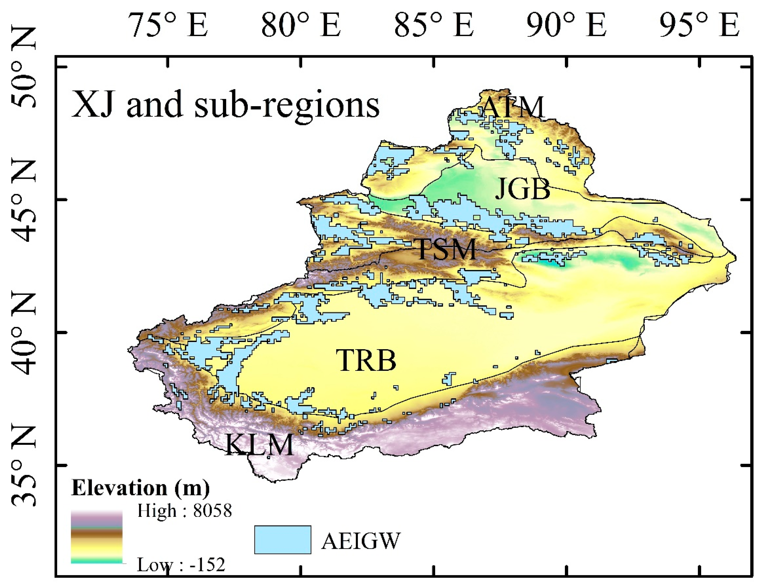
Funding

This research was funded by the Strategic Priority Research Program of Chinese Academy of Sciences, Pan-Third Pole Environment Study for a Green Silk Road (Pan-TPE XDA20060303), the Western Scholars of the Chinese Academy of Sciences (2015-XBQN-B-20), the National Science Foundation of China (Project 71704150), General Research Fund (HKBU 203913) and Early Career Scheme (HKBU 22301916) of Research Grants Council (RGC) of Hong Kong, and Hong Kong Baptist University Faculty Research Grant (FRG2/14-15/073, FRG2/16-17/004 and FRG 2/17-18/030), and the Strategic Priority Research Program of the Chinese Academy of Sciences (XDA20020101).

Acknowledgments

The datasets used in this study are available in the sources listed in Table 1. We thank associate professor Wei Feng and associate professor Zizhan Zhang from the Institute of Geodesy and Geophysics, Chinese Academy of Sciences, and Haijun Deng from the Fujiang Normal University for their assistance during this study. We also thank the editor and reviewers for their valuable comments on this manuscript.

Conflicts of Interest

The authors declare no conflict of interest.

References

  1. Siebert, S.; Burke, J.; Faures, J. Groundwater use for irrigation-a global inventory. Hydrol. Earth Syst. Sci. 2010, 14, 1863–1880. [Google Scholar] [CrossRef]
  2. Famiglietti, J. The global groundwater crisis. Nat. Clim. Change. 2014, 4, 945–948. [Google Scholar] [CrossRef]
  3. Aeschbach-Hertig, W.; Gleeson, T. Regional strategies for the accelerating global problem of groundwater depletion. Nat. Geosci. 2012, 5, 853–861. [Google Scholar] [CrossRef]
  4. Chen, J.; Famiglietti, J.S.; Scanlon, B.R.; Rodell, M. Groundwater Storage Changes: Present Status from GRACE Observations. Surv Geophys. 2016, 37, 397–417. [Google Scholar] [CrossRef]
  5. Hu, Z.; Zhou, Q.; Chen, X.; Qian, C.; Wang, S.; Li, J. Variations and changes of annual precipitation in central Asia over the last century. Int. J. Climatol. 2017, 37, 157–170. [Google Scholar] [CrossRef]
  6. Chen, X.; Wang, S.; Hu, Z. Spatiotemporal characteristics of seasonal precipitation and their relationships with ENSO in Central Asia during 1901–2013. J. Geogr. Sci. 2018, 28, 1341–1368. [Google Scholar] [CrossRef]
  7. Deng, M. Current situation and its potential analysis of exploration and utilization of groundwater resources of Xinjiang (in Chinese). Arid Land Geogr. 2009, 32, 647–654. [Google Scholar]
  8. Hu, R. Physical Geography of the Tianshan Mountains in China; China Environmental Science Press: Beijing, China, 2004; p. 8. [Google Scholar]
  9. Xia, J.; Wu, X.; Zhan, C.; Qiao, Y.; Hong, S.; Yang, P.; Zou, L. Evaluating the Dynamics of Groundwater Depletion for an Arid Land in the Tarim Basin, China. Water. 2019, 11, 186. [Google Scholar] [CrossRef]
  10. Huang, T.; Pang, Z. Changes in groundwater induced by water diversion in the Lower Tarim River, Xinjiang Uygur, NW China: Evidence from environmental isotopes and water chemistry. J. Hydrol. 2010, 387, 188–201. [Google Scholar] [CrossRef]
  11. Zhou, J.; Dong, X.; Li, G.; Wang, Y.; Guo, X. Evaluation of groundwater quality in the Xinjiang Plain Area. Front. Environ. Sci. Engin. China 2010, 4, 183–186. [Google Scholar] [CrossRef]
  12. Chen, X.; Li, B.; Li, Q.; Li, J.; Abdulla, S. Spatio-temporal pattern and changes of evapotranspiration in arid Central Asia and Xinjiang of China. J. Arid Land 2012, 4, 105–112. [Google Scholar] [CrossRef]
  13. Hu, Z.; Zhang, C.; Luo, G.; Teng, Z.; Jia, C. Characterizing cross-scale chaotic behaviors of the runoff time series in an inland river of Central Asia. Quat. Int. 2013, 311, 132–139. [Google Scholar] [CrossRef]
  14. Hu, Z.; Hu, Q.; Zhang, C.; Chen, X.; Li, Q. Evaluation of reanalysis, spatially interpolated and satellite remotely sensed precipitation data sets in central Asia. J. Geophys. Res. Atmos. 2016, 121, 5648–5663. [Google Scholar] [Green Version]
  15. Hu, Z.; Li, Q.; Chen, X.; Teng, Z.; Chen, C.; Yin, G.; Zhang, Y. Climate changes in temperature and precipitation extremes in an alpine grassland of central Asia. Theor. Appl. Climatol. 2016, 126, 519–531. [Google Scholar] [CrossRef]
  16. Rodell, M.; Velicogna, I.; Famiglietti, J. Satellite-based estimates of groundwater depletion in India. Nature 2009, 460, 999–1002. [Google Scholar] [CrossRef] [PubMed] [Green Version]
  17. Famiglietti, J.; Lo, M.; Ho, S.; Bethune, J.; Anderson, K.; Syed, T.; Swenson, S.; Linage, C.; Rodell, M. Satellites measure recent rates of groundwater depletion in California’s Central Valley. Geophys. Res. Lett. 2011, 38, L03403. [Google Scholar] [CrossRef]
  18. Feng, W.; Zhong, M.; Lemoine, J. Evaluation of groundwater depletion in North China using the Gravity Recovery and Climate Experiment (GRACE) data and ground-based measurements. W. Resour. Res. 2013, 49, 2110–2118. [Google Scholar] [CrossRef]
  19. Feng, W.; Shum, C.; Zhong, M. Groundwater Storage Changes in China from Satellite Gravity: An Overview. Remote Sens. 2018, 10, 674. [Google Scholar] [CrossRef]
  20. Frappart, F.; Ramillien, G. Monitoring Groundwater Storage Changes Using the Gravity Recovery and Climate Experiment (GRACE) Satellite Mission: A Review. Remote Sens. 2018, 10, 829. [Google Scholar] [CrossRef]
  21. Han, Z.; Huang, S.; Huang, Q.; Leng, G.; Wang, H.; He, L.; Fang, W.; Li, P. Assessing GRACE-based terrestrial water storage anomalies dynamics at multi-timescales and their correlations with teleconnection factors in Yunnan Province, China. J. Hydrol. 2019, 574, 836–859. [Google Scholar] [CrossRef]
  22. Dong, X.; Deng, M. Xinjiang Groundwater Resources; Xinjiang Science and Technology Press: Xinjiang, China, 2005; pp. 6–8. [Google Scholar]
  23. Chen, X.; Hu, R.; Huang, Y.; Wang, Y.; Ban, W.; Dou, Y.; Yu, M.; Feng, X.; Chen, X. Hydrological Model of Inland River Basin in Arid Land; Environmental Science Press: Beijing, China, 2012; pp. 4–18. [Google Scholar]
  24. Hu, Z.; Zhou, Q.; Chen, X.; Li, J.; Li, Q.; Chen, D.; Liu, W.; Yin, G. Evaluation of three global gridded precipitation data sets in central Asia based on rain gauge observations. Int. J. Climatol. 2018, 38, 3475–3493. [Google Scholar] [CrossRef]
  25. Hu, Z.; Chen, X.; Chen, D.; Li, J.; Wang, S.; Zhou, Q.; Yin, G.; Guo, M. “Dry gets drier, wet gets wetter”: A case study over the arid regions of Central Asia. Int. J. Climatol. 2019, 39, 1072–1091. [Google Scholar] [CrossRef]
  26. Hu, Z.; Zhang, C.; Hu, Q.; Tian, H. Temperature changes in central Asia from 1979–2011 based on multiple datasets. J. Clim. 2014, 27, 1143–1167. [Google Scholar] [CrossRef]
  27. Shi, Y.; Shen, Y.; Kang, E.; Li, D.; Ding, Y.; Zhang, G.; Hu, R. Recent and future climate change in northwest China. Clim. Chang. 2007, 80, 379–393. [Google Scholar] [CrossRef]
  28. Tapley, B.; Bettadpur, S.; Ries, J.; Thompson, P.; Watkins, M. GRACE measurements of mass variability in the Earth system. Science 2004, 305, 503–505. [Google Scholar] [CrossRef] [PubMed]
  29. Wahr, J.; Swenson, S.; Zlotnicki, V.; Velicogna, I. Time-variable gravity from GRACE: First results. Geophys. Res. Lett. 2004, 31, L11501. [Google Scholar] [CrossRef]
  30. Zhao, Y.; Zhu, J.; Xu, Y. Establishment and assessment of the grid precipitation datasets in China for recent 50 years. J. Meteorol. Sci. 2014, 34, 414–420. [Google Scholar]
  31. Taylor, R.G.; Scanlon, B.; Döll, P.; Rodell, M.; Van Beek, R.; Wada, Y.; Longuevergne, L.; Leblanc, M.; Famiglietti, J.S.; Edmunds, M.; et al. Ground Water and climate change. Nat. Clim. Change 2013, 3, 322–329. [Google Scholar] [CrossRef]
  32. Miralles, D.G.; Teuling, A.J.; van Heerwaarden, C.; de Arellano, J. Mega-heatwave temperatures due to combined soil desiccation and atmospheric heat accumulation. Nat. Geosci. 2014, 7, 345–349. [Google Scholar] [CrossRef]
  33. Martens, B.; Miralles, D.G.; Lievens, H.; van der Schalie, R.; de Jeu, R.A.M.; Fernández-Prieto, D.; Beck, H.E.; Dorigo, W.A.; Verhoest, N.E.C. GLEAM v3: Satellite-based land evaporation and root-zone soil moisture. Geosci. Model Dev. 2017, 10, 1903–1925. [Google Scholar] [CrossRef]
  34. Liu, W.; Wang, L.; Zhou, J. A worldwide evaluation of basin-scale evapotranspiration estimates against the water balance method. J. Hydrol. 2016, 538, 82–95. [Google Scholar] [CrossRef] [Green Version]
  35. Strassberg, G.; Scanlon, B.; Chambers, D. Evaluation of groundwater storage monitoring with the GRACE satellite: Case study of the High Plains aquifer, central United States. W. Resour. Res. 2009, 45. [Google Scholar] [CrossRef] [Green Version]
  36. Gu, X.; Zhang, Q.; Li, J.; Singh, V.P.; Liu, J.; Sun, P.; Cheng, C. Attribution of global soil moisture drying to human activities: A quantitative viewpoint. Geophys. Res. L. 2019, 46, 2573–2582. [Google Scholar] [CrossRef]
  37. Werth, S.; White, D.; Bliss, D. GRACE detected rise of groundwater in the Sahelian Niger River basin. J. Geophys. Res. Sol. Earth 2017, 122, 10459–10477. [Google Scholar]
  38. Gu, X.; Li, J.; Chen, Y.D.; Kong, D.; Liu, J. Consistency and discrepancy of global surface soil moisture changes from multiple model-based data sets against satellite observations. J. Geophys. Res. Atmos. 2019, 124, 1474–1495. [Google Scholar] [CrossRef]
  39. Scanlon, B.; Faunt, C.C.; Longuevergne, L.; Reedy, R.C.; Alley, W.M.; McGuire, V.L.; McMahon, P.B. Groundwater depletion and sustainability of irrigation in the US high plains and central valley. PNAS 2012, 109, 9320–9325. [Google Scholar] [CrossRef] [PubMed]
  40. Castellazzi, P.; Longuevergne, L.; Martel, R. Quantitative mapping of groundwater depletion at the water management scale using a combined GRACE/InSAR approach. Remote Sens. Environ. 2018, 205, 408–418. [Google Scholar] [CrossRef]
  41. Zhou, H.; Zhang, J. Analysis on the Volume of Available Water Resources and Its Carrying Capacity in Xinjiang, China. Arid Land Geogr. 2005, 28, 756–763. [Google Scholar]
  42. Yang, T.; Wang, C.; Chen, Y.; Chen, X.; Yu, Z. Climate change and water storage variability over an arid endorheic Region. J. Hydrol. 2015, 529, 330–339. [Google Scholar] [CrossRef]
  43. Deng, H.; Chen, Y. Influences of recent climate change and human activities on water storage variations in Central Asia. J. Hydrol. 2017, 544, 46–57. [Google Scholar] [CrossRef]
  44. Farinotti, D.; Longuevergne, L.; Moholdt, G.; Duethmann, D.; Mölg, T.; Bolch, T.; Vorogushyn, S.; Güntner, A. Substantial glacier mass loss in the Tien Shan over the past 50 years. Nat. Geosci. 2015, 8, 716–722. [Google Scholar] [CrossRef]
  45. Geladi, P.; Kowlaski, B. Partial least square regression: A tutorial. Anal. Chem. Acta 1986, 35, 1–17. [Google Scholar] [CrossRef]
  46. Wold, S.; Sjostrom Mand Eriksson, L. PLS-regression: A basic tool of chemometrics. Chemom. Intel. Lab. Syst. 2001, 58, 109–130. [Google Scholar] [CrossRef]
  47. Grogan, D.; Wisser, D.; Prusevich, A.; Lammers, R.; Frolking, S. The use and re-use of unsustainable groundwater for irrigation: A global budget. Environ. Res. Lett. 2017, 12, 034017. [Google Scholar] [CrossRef]
  48. Tweed, S.; Celle-Jeanton, H.; Cabot, L.; Huneau, F.; De Montety, V.; Nicolau, N.; Travi, Y.; Babic, M.; Aquilina, L.; Vergnaud-Ayraud, V.; et al. Impact of irrigated agriculture on groundwater resources in a temperate humid region. Sci. Total Environ. 2018, 613, 1302–1316. [Google Scholar] [CrossRef] [PubMed]
Figure 1. Study area: Xinjiang (XJ) and the locations of the five sub-regions, i.e., Altain Mountainous (ATM), Junggar Basin (JGB), Tianshan Mountainous (TSM), Tarim Basin (TRB) and Kunlun Mountainous (KLM). The black line denotes the boundary of the sub-regions. The blue represents the area of irrigation from groundwater, which are extracted from the Global Map of Irrigation Areas (GMIA) V5.0 of the Food and Agriculture Organization of the United Nations, AEIGW: Area equipped for irrigation with groundwater.
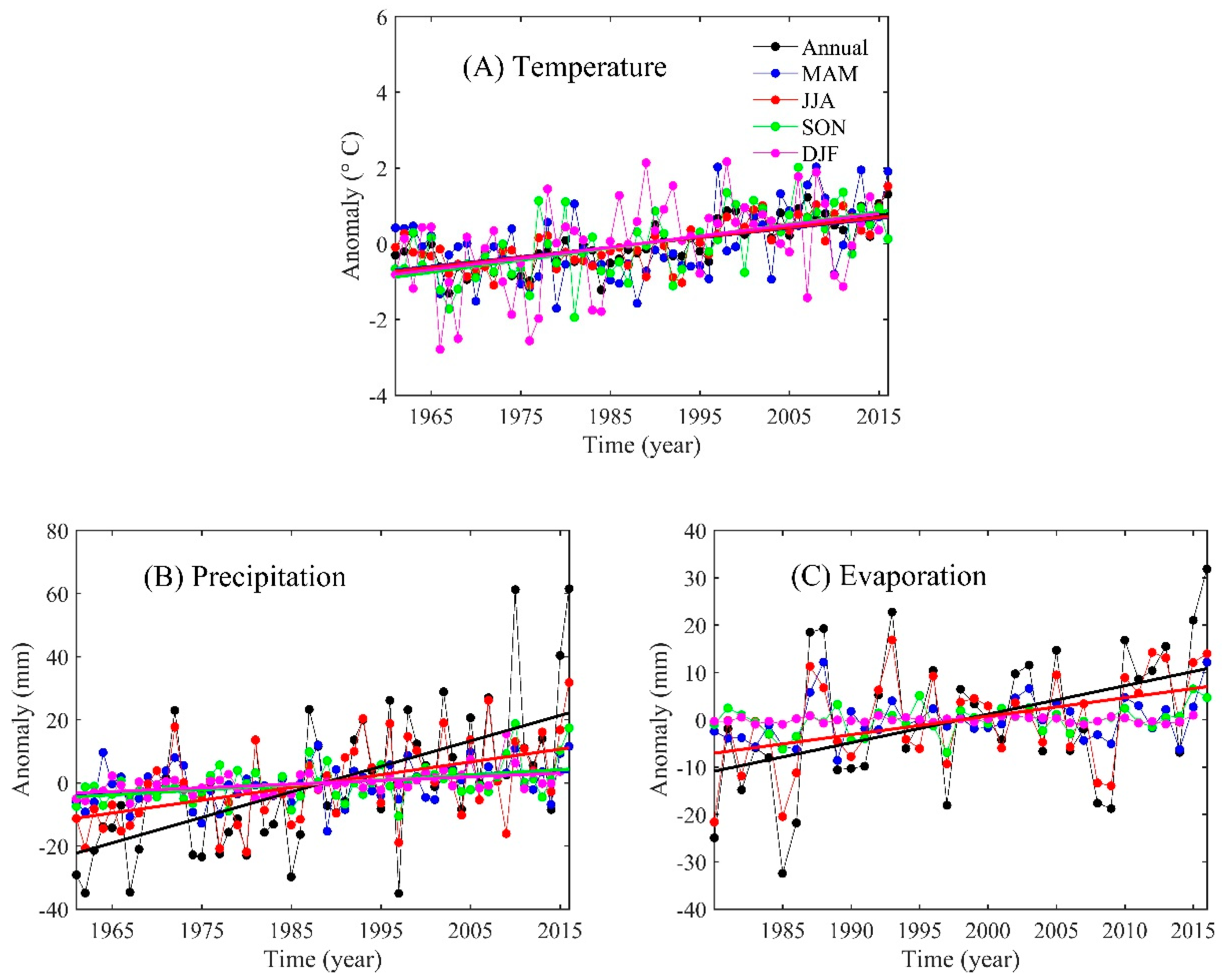
Remotesensing 11 01908 g001
Figure 2. Annual and seasonal temperature anomalies (A), precipitation anomalies (B) during 1961–2016 and evaporation anomalies (C) during 1980–2016. The bold lines are the linear trends. Only linear trends significant at the 95% (or 99%) significance level are shown.
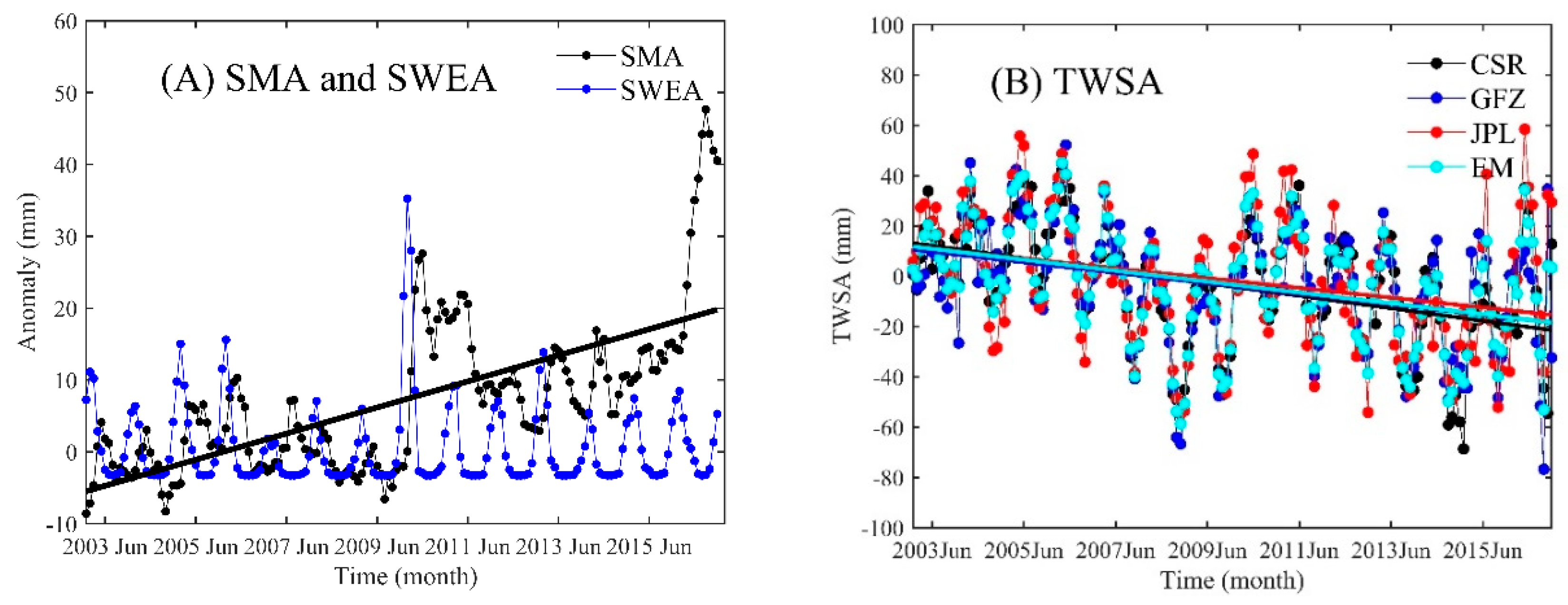
Remotesensing 11 01908 g002
Figure 3. Monthly Soil Moisture Anomalies (SMA), Snow Water Equivalent Anomalies (SWEA) (A) and Terrestrial Water Storage Anomalies (TWSA) (B) over Xinjiang during 2003–2016.
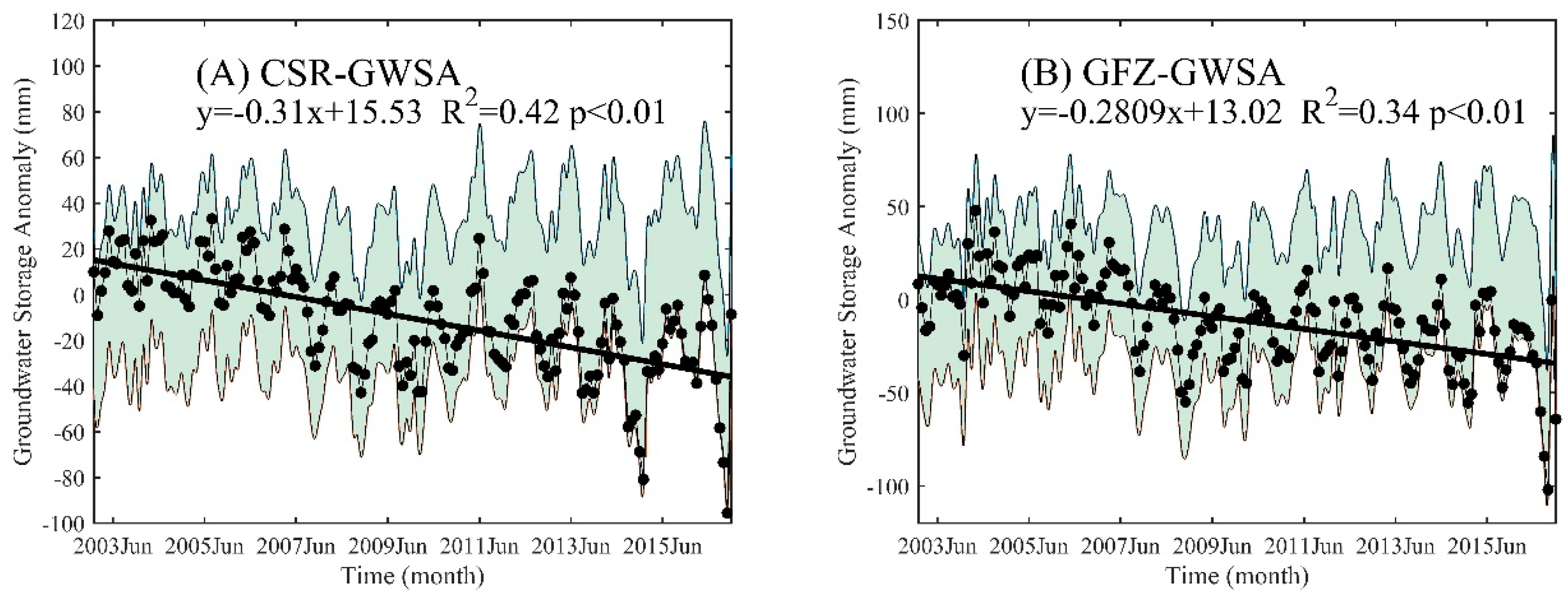
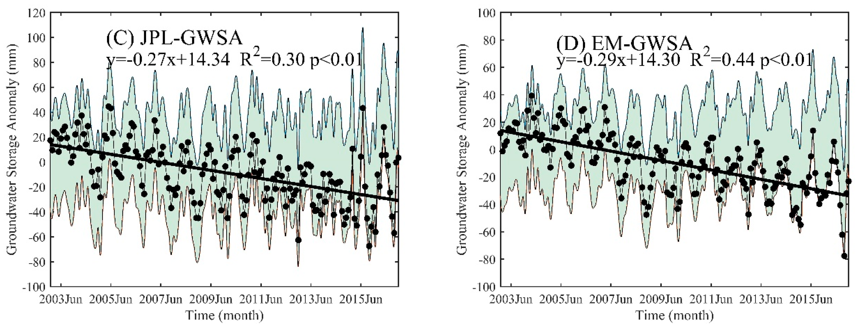
Remotesensing 11 01908 g003
Figure 4. Monthly Groundwater Storage Anomalies (GWSA) derived from Centre for Space Research (CSR), (A), Geo Forschungs Zentrum (GFZ) (B), Jet Propulsion Laboratory (JPL) (C), and ensemble mean (EM) (D) in Xinjiang during 2003–2016. The black dots are monthly GWSA. The bold lines denote linear trends. The shading areas denote the 95% significance interval.
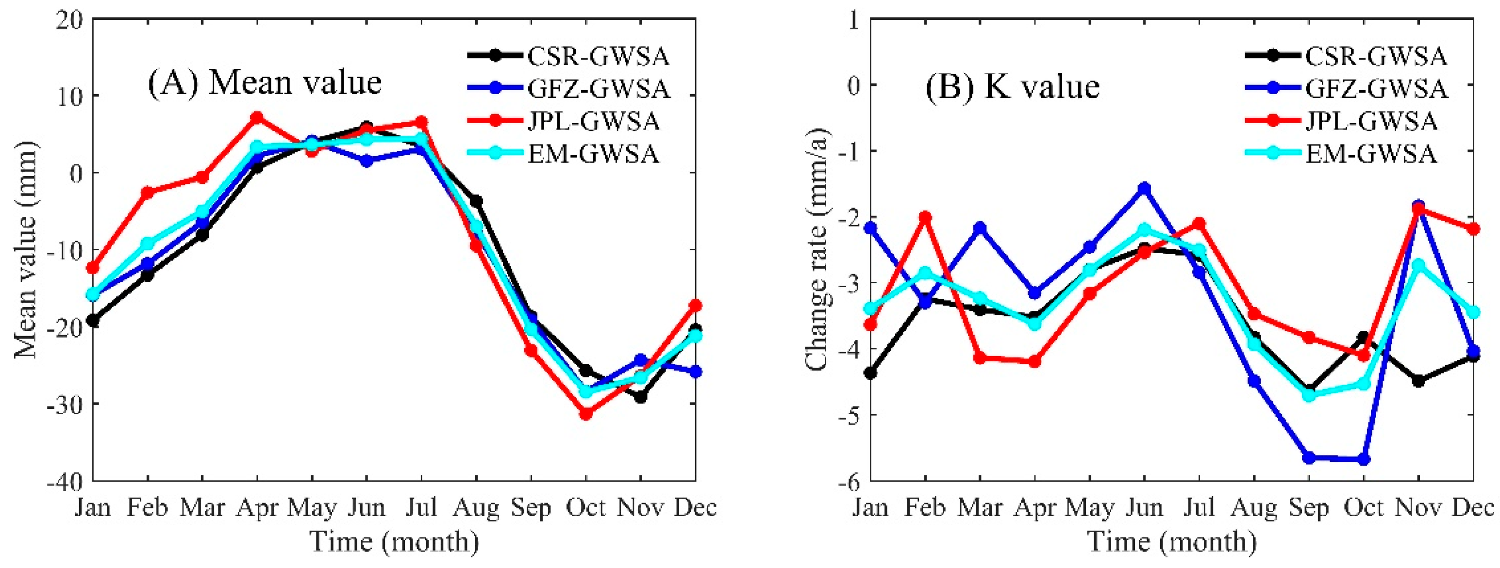
Remotesensing 11 01908 g004aRemotesensing 11 01908 g004b
Figure 5. Average (mm; A) and linear trend (mm/a; B) of monthly Groundwater Storage Anomalies (GWSA) in Xinjiang over 2003–2016.
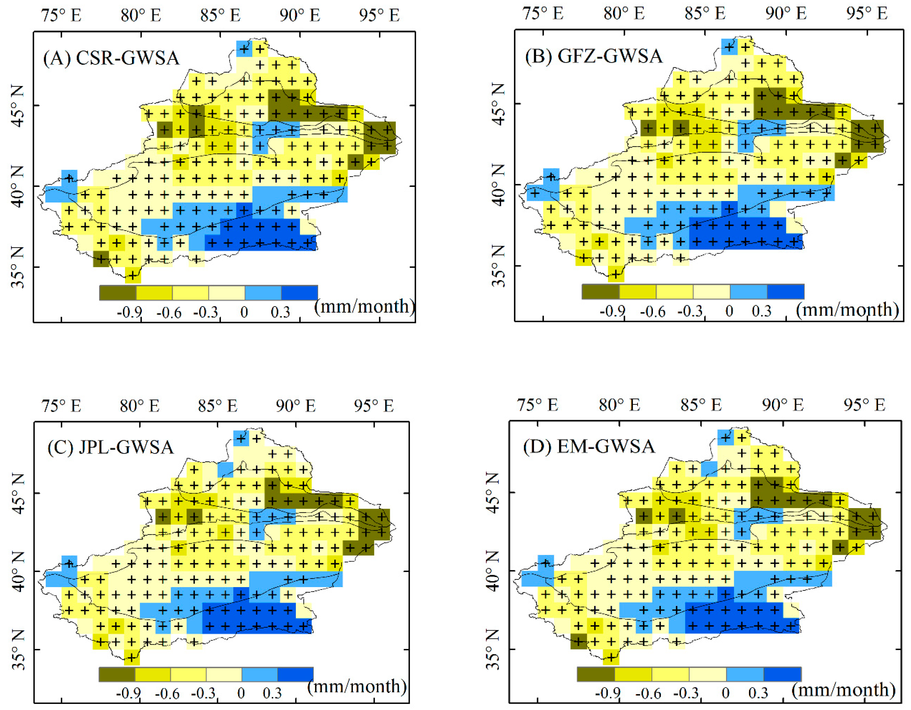
Remotesensing 11 01908 g005
Figure 6. Spatial distributions of the linear trends (mm/month) of the monthly GWSA during 2003–2016. The cross signs denote the trends are significant at the 95% significance level.
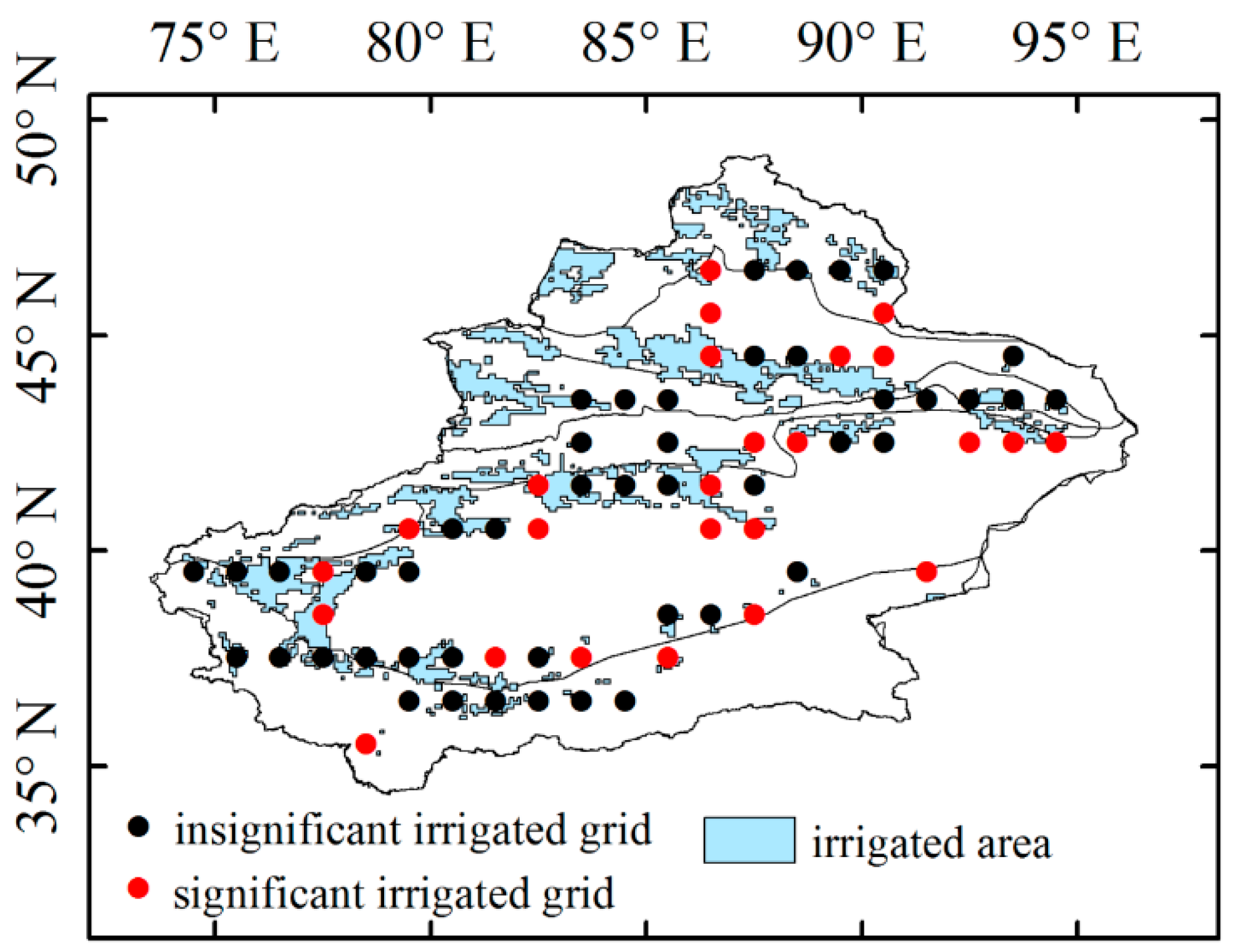
Remotesensing 11 01908 g006
Figure 7. Comparison between the irrigated grids and the matched non-irrigated grids based on the annual EM-GWSA dataset. Results of Student’s t test of annual EM-GWSA between irrigated grids and their surrounding non-irrigated grids. The red dots represent irrigated grids with significant different GWSA from their surrounding non-irrigated grids, and the black dots represent their differences are insignificant. The blue areas are irrigated areas.
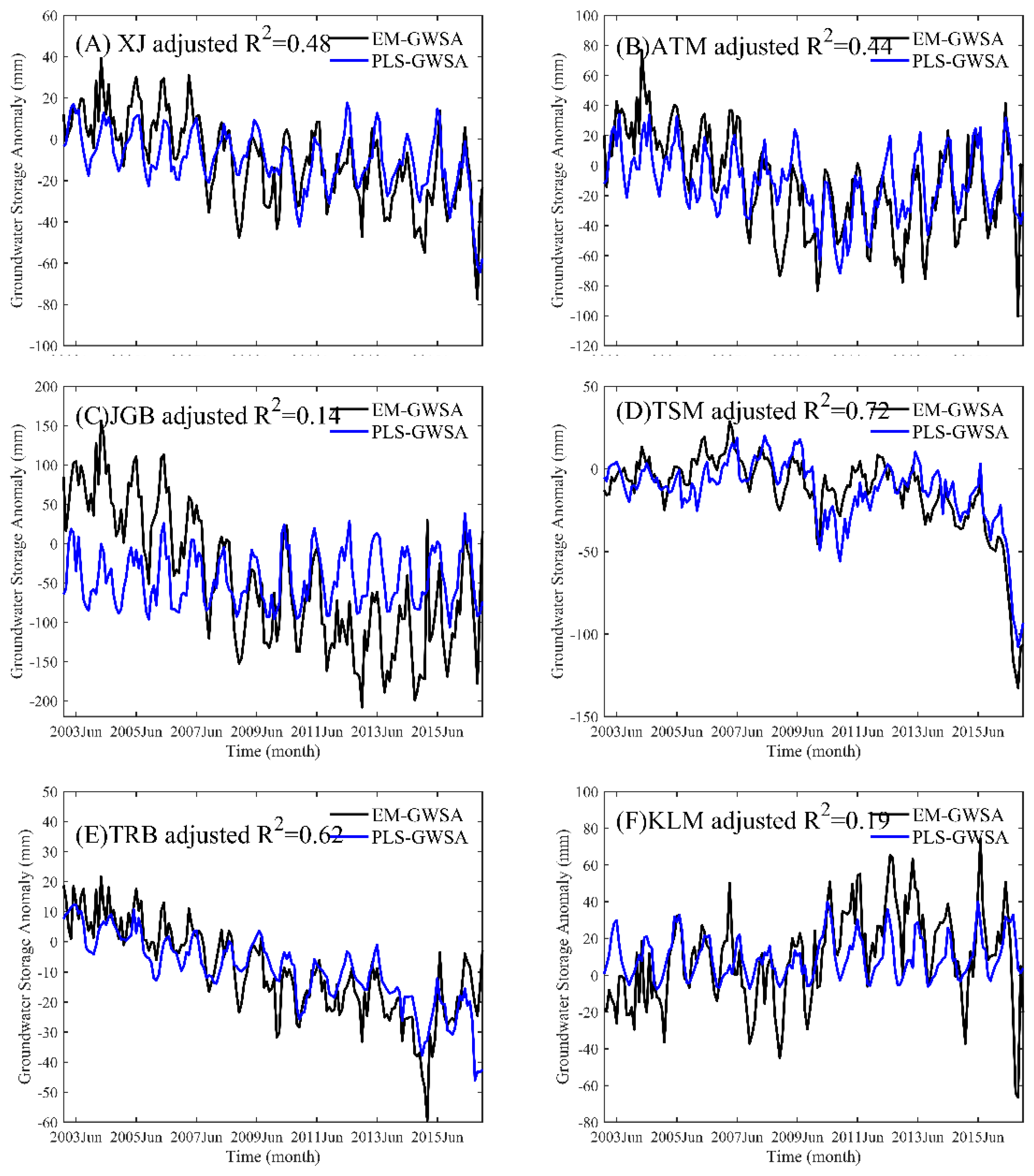
Remotesensing 11 01908 g007
Figure 8. Monthly time series of EM-GWSA and partial least squares (PLS)-GWSA during 2003–2016 in XJ (A), ATM (B), JGB (C), TSM (D), TRB (E) and KLM (F).
Remotesensing 11 01908 g008
Table 1. Datasets used in this study.
VariableAcronymPeriodSpatial ResolutionSource
Terrestrial Water Storage AnomaliesTWSA2002.04–2017.01 (monthly)1° × 1°Jet Propulsion Laboratory, California Institute of Technology https://grace.jpl.nasa.gov/data/get-data/
PrecipitationP1961–2017 (monthly)0.5° × 0.5°China Meteorological Administration http://data.cma.cn/site/index.html
TemperatureT1961–2017 (monthly)0.5° × 0.5°China Meteorological Administration http://data.cma.cn/site/index.html
EvaporationE1980–2016 (daily)0.25° × 0.25°Global Land Evaporation Amsterdam Model V3.1a https://www.gleam.eu/
Soil MoistureSM2000–2017 (monthly)1° × 1°GLDAS Noah Land Surface Model L4 2.1 https://search.earthdata.nasa.gov/
Snow Water EquivalentSWE2000–2017 (monthly)1° × 1°GLDAS Noah Land Surface Model L4 2.1 https://search.earthdata.nasa.gov/
Observed Groundwater RechargeOBS-GWR2003–2015 (annual)Regional averageXinjiang Water Resources Bulletin http://www.xjslt.gov.cn/zwgk/slgb/index.html
Observed Groundwater DepthGWD2004–2010 (monthly)Point (41.79° N, 81.62° E)Department of Water Resources of Xinjiang Uygur Autonomous Region http://www.xjslt.gov.cn
Table 2. Change rates of gravity recovery and climate experiment (GRACE)-based GWSA at different timescales (mm/month for monthly scale, mm/a for seasonal and annual scales) during 2003–2016. ** denotes the trend is significant at the 95% or 99% confidence level. ± values are the 5% and 95% significance intervals.
TimescaleCSR-GWSAGFZ-GWSAJPL-GWSAEM-GWSA
Monthly−0.31 ** ± 0.06−0.28 ** ± 0.06−0.27 ** ± 0.06−0.29 ** ± 0.05
MAM−3.24 ** ± 1.27−2.59 ** ± 2.02−3.83 ** ± 1.78−3.22 ** ± 1.35
JJA−2.96 ** ± 1.05−2.96 ** ± 1.51−2.70 ** ± 1.61−2.88 ** ± 0.84
SON−4.32 ** ± 2.21−4.39 ** ± 1.85−3.27 ** ± 1.26−3.99 ** ± 1.25
DJF−4.61 ** ± 1.71−3.06 ** ± 1.97−2.99 ** ± 2.19−3.55 ** ± 1.57
Annual−3.61 ** ± 0.85−3.28 ** ± 1.04−3.10 ** ± 0.91−3.33 ** ± 0.74
Table 3. Correlation coefficients (CC) of CSR-GWSA, GFZ-GWSA, JPL-GWSA, and EM-GWSA at monthly, seasonal and annual scales in 2003–2016. All CC values are significant at the 99% confidence level using the Student’s t-test.
Time ScaleDatasetCSR-GWSAGFZ-GWSAJPL-GWSAEM-GWSA
MonthlyCSR-GWSA1.00
GFZ-GWSA0.761.00
JPL-GWSA0.690.631.00
EM-GWSA0.910.900.871.00
MAMCSR-GWSA1.00
GFZ-GWSA0.741.00
JPL-GWSA0.880.631.00
EM-GWSA0.960.860.931.00
JJACSR-GWSA1.00
GFZ-GWSA0.831.00
JPL-GWSA0.530.551.00
EM-GWSA0.900.910.801.00
SONCSR-GWSA1.00
GFZ-GWSA0.841.00
JPL-GWSA0.630.731.00
EM-GWSA0.930.950.831.00
DJFCSR-GWSA1.00
GFZ-GWSA0.921.00
JPL-GWSA0.720.591.00
EM-GWSA0.970.920.841.00
AnnualCSR-GWSA1.00
GFZ-GWSA0.941.00
JPL-GWSA0.920.841.00
EM-GWSA0.990.960.951.00
Table 4. Linear trends (mm/a) of seasonal and annual EM-GWSA over five sub-regions [i.e., Altain Mountainous (ATM), Junggar Basin (JGB), Tianshan Mountainous (TSM), Tarim Basin (TRB) and Kunlun Mountainous (KLM)] in 2003–2016, * and ** significant at the 95% and 99% confidence level, respectively.
Sub-RegionsMAMJJASONDJFANN
ATM−0.24 *−0.27 **−0.38 ** −0.32 *−3.84 **
JGB−1.27 ** −1.09 **−1.18 **−1.20 **−15.27 **
TSM−0.20 *−0.30 *−0.40 **−0.21 *−3.74 **
TRB−0.23 **−0.19 ** −0.21 **−0.26 ** −2.93 **
KLM0.20 *0.24 *0.080.14 2.2 *
Table 5. Population, cultivated land area, agricultural water use, groundwater abstraction, groundwater recharge, total water use, groundwater abstract/groundwater resources, and groundwater abstract/total water use over Xinjiang during 2003–2016.
YearPopulation (Million) Cultivated Land Area (1000 km2) Agricultural Water Use (m3/m2)Groundwater Abstraction (billion m3)Groundwater Recharge (billion m3)Total Water Use (billion m3)Groundwater Utilization/Groundwater Resources (%)Groundwater Abstraction/Total Water Use (%)
200319.3334.401.235.360.4349.448.78 10.73
200419.6334.251.115.850.2649.6411.44 11.59
200520.1030.671.005.956.2650.8310.42 11.54
200620.5038.280.965.955.4151.3710.64 11.47
200720.9534.320.966.851.4151.7713.18 13.09
200821.3145.370.918.051.8552.8215.40 15.12
200921.5947.720.949.047.0953.0919.10 16.94
201021.8547.590.929.562.4353.5115.24 17.78
201122.0949.840.819.853.9852.3518.11 18.67
201222.3351.370.9611.155.7059.0119.91 18.79
201322.6452.120.9311.056.1358.8119.67 18.77
201422.9859.950.9313.144.3958.1829.59 22.58
201523.6061.260.8911.953.6357.7222.26 20.69
201623.9862.32-- --
Table 6. Regression coefficients of the monthly EM-GWSA as the function of precipitation anomalies (PA), temperature anomalies (TA), evaporation anomalies (EA), SMA and SWEA by the partial least squares regression (PLSR) method over the six regions in 2003-2016.
Regression CoefficientXJATMJGBTSMTRBKLM
a 0 −4.68−5.13−47.82−1.97−2.656.86
a 1 −0.51−0.23−1.04−0.310.260.01
a 2 −0.92−1.99−1.92−1.250.16−0.75
a 3 2.472.014.121.250.931.58
a 4 −0.98−0.650.04−1.57−1.670.09
a 5 −0.15−0.32−0.57−0.87−0.770.18
Table 7. Adjusted R2 results of the PLSR over six regions: Xinjiang (XJ) and the locations of the five sub-regions, i.e., Altain Mountainous (ATM), Junggar Basin (JGB), Tianshan Mountainous (TSM), Tarim Basin (TRB) and Kunlun Mountainous (KLM) at the three cases.
XJATMJGBTSMTRBKLM
Case 10.48 0.44 0.14 0.72 0.62 0.19
Case 20.25 0.24 0.15 0.06 0.05 0.19
Case 30.11 0.08 0.01 0.59 0.49 0.03
Table 8. Correlation coefficients (CC) between annual EM-GWSA and other annual hydroclimatic variables (PA, TA, EA, SMSA, SWESA) over six regions in 2003–2016, ** and * indicate significance at 99% and 95% confidence levels, respectively.
Study AreaPATAEASMASWEA
XJ0.26 **0.31 **0.44 **−0.32 **−0.10
ATM0.110.29 **0.46 **−0.19 *−0.25 **
JGB0.15 *0.20*0.36 **0.07−0.11
TSM0.030.100.15−0.75 **−0.10
TRB0.17 *0.26 **0.19 *−0.67 **−0.10
KLM0.28 **0.29 **0.42 **0.21 **−0.03

