Airborne Lidar Sampling Strategies to Enhance Forest Aboveground Biomass Estimation from Landsat Imagery


1
Department of Environmental Resources Engineering, State University of New York College of Environmental Science and Forestry, Syracuse, NY 13210, USA
2
School of Urban and Environmental Engineering, Ulsan National Institute of Science and Technology, Ulsan 44919, Korea
*
Author to whom correspondence should be addressed.
Remote Sens. 2019, 11(16), 1906; https://doi.org/10.3390/rs11161906
Submission received: 2 July 2019
/
Revised: 10 August 2019
/
Accepted: 12 August 2019
/
Published: 15 August 2019
(This article belongs to the Special Issue Advances in Active Remote Sensing of Forests)
Abstract
:Accurately estimating aboveground biomass (AGB) is important in many applications, including monitoring carbon stocks, investigating deforestation and forest degradation, and designing sustainable forest management strategies. Although lidar provides critical three-dimensional forest structure information for estimating AGB, acquiring comprehensive lidar coverage is often cost prohibitive. This research focused on developing a lidar sampling framework to support AGB estimation from Landsat images. Two sampling strategies, systematic and classification-based, were tested and compared. The proposed strategies were implemented over a temperate forest study site in northern New York State and the processes were then validated at a similar site located in central New York State. Our results demonstrated that while the inclusion of lidar data using systematic or classification-based sampling supports AGB estimation, the systematic sampling selection method was highly dependent on site conditions and had higher accuracy variability. Of the 12 systematic sampling plans, R2 values ranged from 0.14 to 0.41 and plot root mean square error (RMSE) ranged from 84.2 to 93.9 Mg ha−1. The classification-based sampling outperformed 75% of the systematic sampling strategies at the primary site with R2 of 0.26 and RMSE of 70.1 Mg ha−1. The classification-based lidar sampling strategy was relatively easy to apply and was readily transferable to a new study site. Adopting this method at the validation site, the classification-based sampling also worked effectively, with an R2 of 0.40 and an RMSE of 108.2 Mg ha−1 compared to the full lidar coverage model with an R2 of 0.58 and an RMSE of 96.0 Mg ha−1. This study evaluated different lidar sample selection methods to identify an efficient and effective approach to reduce the volume and cost of lidar acquisitions. The forest type classification-based sampling method described in this study could facilitate cost-effective lidar data collection in future studies.
1. Introduction
Forest ecosystem management requires comprehensive, timely, and accurate monitoring efforts [1]. Above ground biomass (AGB) is an important indicator in monitoring the change of forest carbon stocks. Airborne lidar has been applied successfully to estimate forest biophysical parameters and has provided accurate AGB estimation in many studies [2,3], particularly when used in coordination with data from passive sensors. Commonly used remote sensing data sources, such as Landsat [4], Moderate Resolution Imaging Spectroradiometer (MODIS) [5], and radar [6], tend to reach a saturation point that limits their effectiveness in estimating higher AGB levels [7]. The saturation level of radar varies with the bands applied. For example, X- and C-band backscatter saturates at low biomass levels (30–50 Mg ha−1) [5] and L-band saturation ranges from 40–150 Mg ha−1 [8]. Lidar does not suffer from this saturation problem and thus is able to more accurately estimate AGB [9]. However, lidar acquisitions are often practically limited by cost or data volume. Although the increasing availability of unmanned aerial vehicles (UAVs) are providing new avenues for data collection, the cost and effort to acquire airborne lidar data are still higher than passive satellite sensors like Landsat, MODIS, or Sentinel. Moreover, acquiring full coverage lidar is often infeasible for large area studies due to the data volume. Kelly and Di Tommaso [10] provide an example of a 5 hectare forest stand that can be covered by a 300 byte Landsat Thematic Mapper (TM) image or a 50 Mb 10 pulse/m2 lidar dataset. These cost and data limitations inhibit the widespread and ready availability of lidar data.
Sensors like those onboard the Landsat satellites can provide extensive forest coverage with low cost but offer limited capacity for vertical characterization. Conversely, lidar can provide accurate measurements of forest attributes in the vertical plane; however, as mentioned above, lidar acquisitions are often limited in horizontal extent due to issues with cost and data volume. Additionally, lidar cannot capture all necessary forest attributes. For example, Erdody and Moskal [11] discussed the limitation of lidar data in discerning tree species. To mitigate the weaknesses of each data type, the fusion of lidar and Landsat has been proposed and explored for AGB estimation [4,12]. The advantages of lidar and Landsat data fusion are twofold: (1) Synergistic harnessing of advantages from both datasets, and (2) with appropriate sampling, full lidar coverage is not required.
Researchers have applied lidar sampling to mitigate the limitations associated with managing cost and data volume. Instead of collecting full-coverage data, lidar sampling can significantly reduce the time and effort needed for data collection, organization, and processing. Lidar samples supply detailed information on specific locations that can be used to calibrate models to derive forest attributes for other regions [13]. Studies have demonstrated that lidar sampling can provide estimates for biomass [14,15] or forest height [16]. Researchers have used numerous statistical methods to extrapolate forest biophysical parameters beyond lidar samples to represent a broader area of interest. For example, Boudreau et al. [17] used intermediate samples of airborne lidar data to extrapolate AGB estimates from plot-level forest inventory data to a broader spaceborne lidar coverage. In a two-stage method, they first developed a lidar-based biomass equation to relate plot-level biomass and airborne lidar derived variables and then applied the equation to estimate biomass throughout the airborne lidar coverage. The second stage developed a regression equation between the lidar derived biomass and spaceborne ICESat Geoscience Laser Altimer System (GLAS) metrics in order to extrapolate the limited lidar biomass estimates to the broader GLAS coverage.
There are two approaches to reduce lidar data volume—thinning lidar density and reducing lidar extent—that have proved to have minimal impact on accuracy estimation of biophysical parameters compared with using full lidar data coverage. For example, Holmgren [18] reduced laser density from 4.3 to 0.1 pulses/m2 and observed minimal change in errors for estimation of mean tree height, basal area, and stem volume. This was also confirmed by Maltamo et al. [3] who reported that simulated point density reduction had no effect on volume estimation accuracy. Instead of using full lidar data coverage, Chen and Hay [19] sampled 17.6% of total lidar extent and achieved similar accuracies as the full lidar data in estimating canopy height.
Decisions regarding lidar sample locations are critical. Countless lidar samples can be generated with similar data collecting efforts but may generate different analysis outcomes. It is preferable to use lidar samples that best characterize the study area in order to achieve similar outcomes as comprehensive lidar coverage. Sampling methods used to reduce lidar coverage generally fall into two categories: Systematic sampling and classification-based sampling. In systematic lidar sampling, data are collected based on a designated sampling unit and distance interval. The distribution of sampling units may be point, strip, or grid based. Tsui et al. [20] sampled lidar data using a grid pattern in which horizontal and vertical lines had distance intervals of 1000 m. Hudak et al. [16] sampled lidar data using both strip and point patterns with distance intervals of 250 m, 500 m, 1000 m, and 2000 m. Systematic sampling is easy to design and apply but it might fail to represent the full data range, especially if only a small portion of data are sampled. Classification-based sampling can help compensate for this situation by better representing all value ranges. In classification-based sampling, a classification map is created and then applied to assist lidar sample selection. Chen and Hay [19] aimed to model forest canopy height from lidar samples that were selected by combining pseudo-height classification from QuickBird imagery with several other inputs in a rule-based model. The rules included non-overlapping transects, covering all height classes, and selecting pseudo-height histograms with the highest correlation to the pseudo-height histogram derived from all data. Previous studies have considered both systematic sampling and classification-based sampling, though there has not been a comparison of these two strategies.
The overall aim of this study was to deepen our understanding of lidar sampling for AGB estimation. While the value of lidar sampling has been well documented and various lidar sampling strategies have been proposed, there are no widely accepted protocols for cost-effective lidar sampling for AGB estimation. Additionally, while forest type has long been recognized as a factor in AGB estimation, prior studies have not documented the use of forest type classification for lidar sampling selection within this field. This paper presents a methodological framework to map AGB in temperate forests by combining ground-based inventory data, comprehensive Landsat data, and lidar samples acquired using a variety of methods. We particularly focused on: (1) Assessing whether lidar samples can substitute for comprehensive lidar data collection, (2) characterizing the differences in AGB estimation based on systematic and classification-based sampling lidar sampling strategies, and (3) providing a protocol for lidar sampling acquisition, implementation, and evaluation.
2. Data and Methods
2.1. Study Areas
2.1.1. Main Study Area: Huntington Wildlife Forest
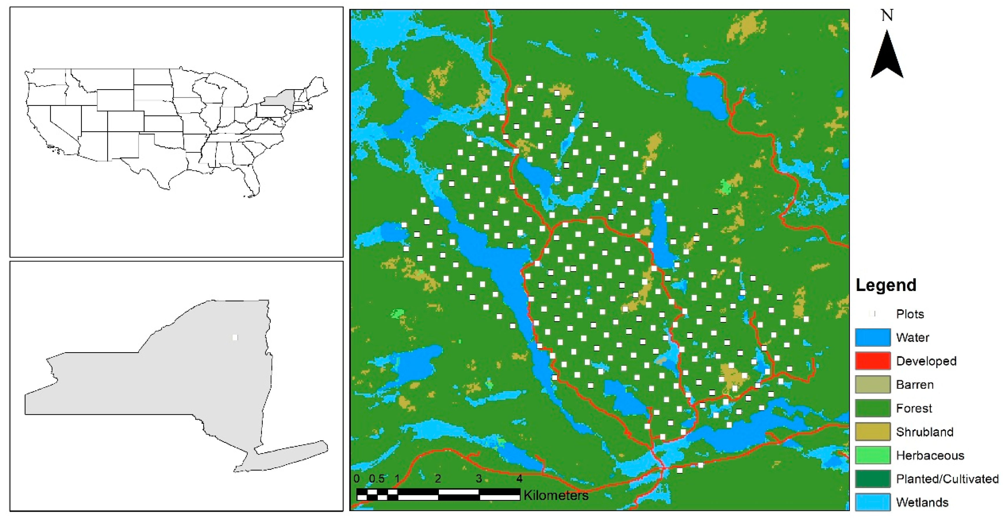
Our main study area was the Huntington Wildlife Forest (Huntington) in the central Adirondack Park in northern New York State. The Huntington property provided a location for evaluating the value of different lidar sampling procedures and developing a sampling protocol. Huntington is managed by the State University of New York College of Environmental Science and Forestry (SUNY ESF; 43°58′19″N, 74°13′18″W; Figure 1). Huntington covers approximately 60 km2 with mountainous topography ranging in elevation from 466 m to 859 m above mean sea level. Huntington had a mean annual temperature of 4.4 °C and mean annual precipitation of 1010 mm [21]. Huntington contained both undisturbed natural communities and managed forest stands with major species being American beech (Fagus grandifolia), yellow birch (Betula alleghaniensis Britt.), sugar maple (Acer saccharum Marshall.), red spruce (Picea rubens Sarg.), red maple (Acer rubrum L.), and hemlock (Tsuga spp.).
2.1.2. Test Study Area: Heiberg Memorial Forest
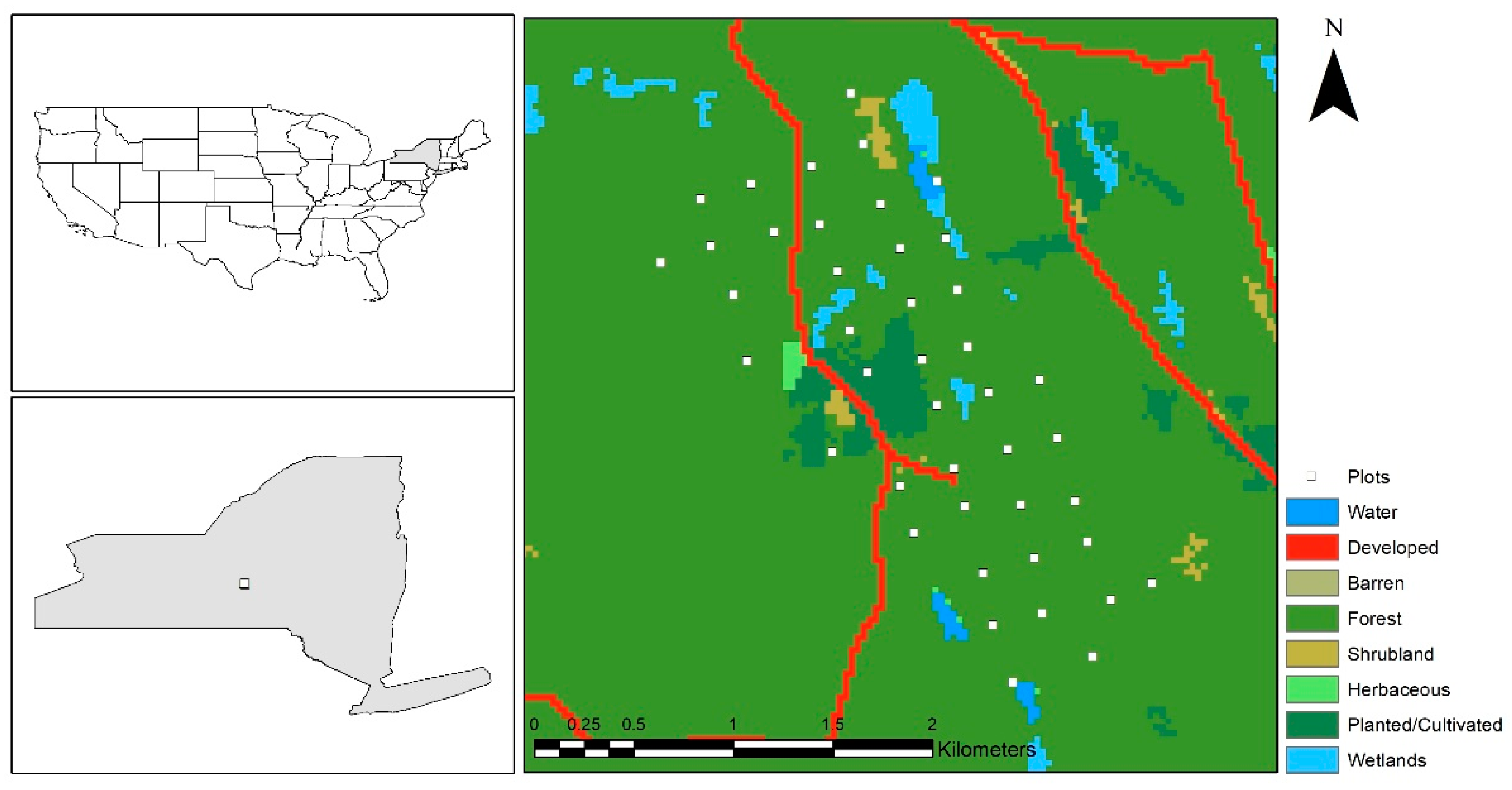
Our test study area was the Heiberg Memorial Forest (Heiberg) south of Syracuse in central New York State. Heiberg is also managed by SUNY ESF (42°47′12″N, 76°05′37″W; Figure 2). Heiberg provided an independent site for testing the lidar sampling protocol developed at Huntington. Heiberg covers approximately 16 km2 with elevation ranging from 383 m to 625 m above mean sea level. The majority of Heiberg was conifer plantations (6.64 km2, 42%), Allegheny hardwoods (5.65 km2, 36%), or open areas (2.39 km2, 15%). Predominant conifer species included Norway spruce (Picea abies), hemlock (Tsuga), white pine (Pinus strobus) and eastern larch (Larix laricina). Deciduous tree species mainly included maple (Acer), ash (Fraxinus L.), beech (Betula), and basswood (T. americana).
2.2. Field Inventory Data
SUNY ESF maintained continuous forest inventory (CFI) plots within Huntington and Heiberg forests, with comprehensive data collected during the summer of 2011 and 2010, respectively. The CFI plots are approximately 405 m2 circular regions, with the center of each plot located using a global positioning system receiver. All trees in the plot with a diameter at breast height (DBH) of 11.7 cm or greater were measured in Huntington and 9.1 cm or greater were measured in Heiberg. The information recorded for each tree included tree species, DBH, and location relative to the plot center.
Based on the field observations, tree-level AGB was calculated using species-specific DBH allometric equations from Jenkins et al. [23]. Plot-level AGB was calculated as the average AGB per unit area within each plot in megagrams per hectare (Mg ha−1). This was calculated by dividing the tree-level AGB total by the plot area. The United Nations Economic Commission for Europe (UNECE) Food and Agriculture Organization (FAO) [24] defined a stand as a mixed forest where neither broadleaved nor coniferous trees account for more than 75% of the tree crown area. We adapted the UNECE/FAO approach and defined a plot as hardwood if the hardwood AGB within the plot was over 75% of the total AGB. Softwood plots were similarly defined when at least 75% of the total AGB was softwood AGB. Mixed forest plots had neither softwood nor hardwood accounting for more than 75% of the total AGB. Table 1 provides descriptive statistics for plot level AGB in hardwood, softwood, and mixed plots in Huntington and Heiberg forests.
2.3. Lidar Data and Processing
Airborne lidar data were acquired for Huntington and Heiberg on 10 September 2011 and 10 August 2010, respectively. ALS60 lidar systems were used to simultaneously collect both discrete return point clouds and the waveforms of the returned signals. Characteristics of the lidar data collections for Huntington and Heiberg are summarized in Table 2. Raw laser data was post-processed by Kucera International using Terrasolid’s TerraScan software [25]. All further point-cloud processing tasks were performed within FUSION software [26].
2.4. Landsat Data and Processing
We selected orthorectified Landsat TM Level-1 images acquired on 19 August 2011 (path/row: 15/29) and 18 July 2010 (path/row: 15/30) that covered the Huntington and Heiberg forest areas, respectively. The images were downloaded from the U.S. Geological Survey Earth Explorer [28]. Although the Landsat images were collected earlier in the growing season than the lidar datasets, they were the cloud-free images that best coincided with the forest inventory data collection.
Using the metadata associated with the downloaded Landsat images, radiometric correction was applied to convert digital numbers into reflectance aiming to mitigate the impact of scene illumination and viewing geometry. Dark object subtraction was applied for atmosphere correction, which was intended to remove the effects of atmosphere scattering and absorption. Radiometric and atmosphere correction were both performed using ENVI 5.2 [29]. Landsat bands 1–5 and 7 (blue, green, red, near infrared, and 2 shortwave infrared), reflectance values, and vegetation indices calculated from these bands were used for model variable selection. Five commonly used vegetation indices were applied in this study: Differenced Vegetation Index (DVI), Ratio Vegetation Index (RVI), Normalized Vegetation Difference Index (NDVI), Soil Adjusted Vegetation Index (SAVI), and Modified Soil Adjusted Vegetation Index (MSAVI) (Table 4).
2.5. Lidar and Landsat Fusion Procedure
2.5.1. Overview
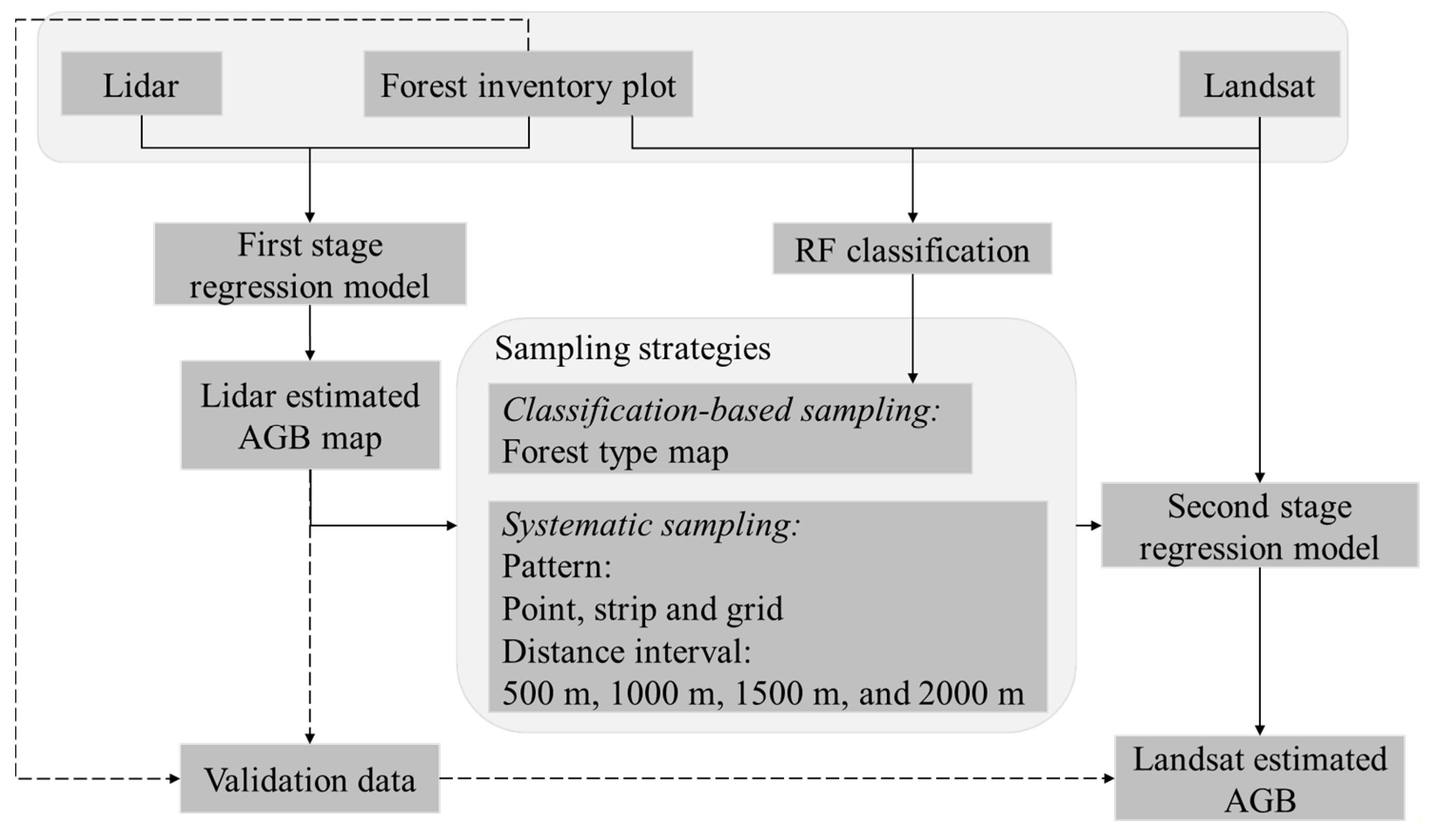
We used AGB data developed from full lidar coverage as a baseline to see if Landsat-based AGB models that used lidar samples could achieve accuracies that approached that of models that used the more expensive full lidar coverage. We also sought to determine how accuracy varied with sampling strategy and if there was a way to establish a protocol to guide lidar sample collection. The workflow for this study is shown in Figure 3. The baseline for comparison in our study was an AGB model developed from the comprehensive lidar data coverage. Forest inventory plot and lidar data were applied to build a first stage regression model that was then used to estimate AGB for the Huntington study area. The impact of different lidar sampling strategies was explored using second stage regression models, which established a relationship between samples of the lidar estimated AGB values and Landsat derived variables. Two categories of lidar sampling strategies were explored: Systematic sampling and classification-based sampling. The classification-based sampling approach was based on a Random Forest (RF) forest type classification. A study previously performed at the same site found that RF had better performance in forest type classification than support vector machine and decision tree algorithms [35]. To assess the accuracy of different sampling strategies, Landsat estimated AGB values generated from second stage regression models were validated using plot and lidar estimated AGB values using mean absolute error (MAE), root mean square error (RMSE), and relative root mean square error (RRMSE). Lidar estimated AGB values covering the full study area were estimated using the first stage regression model and used for testing the Landsat estimated AGB values.
2.5.2. Regression and Variable Selection
This study explored the relationship between AGB and remote sensing derived variables using regression models based on the equation below:
where is the intercept, are model coefficients, and represents the remote sensing derived predictors. As discussed in the prior section, regression models were built in two distinct steps within the workflow (Figure 3). In the first stage regression model, the dependent variable was AGB for the 270 plots within the Huntington area and the predictors were selected from lidar derived variables using the forward variable selection method. Like prior studies [36,37], using the natural logarithm of both dependent and predictor variables led to better performance for the first stage regression model. The second component of the analysis applied Equation (1) to develop regression models for a series of different sampling strategies (described in the next section). Shown as second stage regression models in Figure 3, these models used a sample of the lidar estimated AGB values as the dependent variable and Landsat variables as predictors without variable selection. All variables were used to facilitate comparison by ensuring all second stage regression models had the same predictors.
There are several commonly used variable selection methods when applying multiple linear regression: Forward, backward, and stepwise selection. Forward selection starts with the most significant variable in the model and sequentially adds the next most significant variable into the model until none of the remaining variables are significant. Backward selection starts with all variables in the model and successively removes the least significant variable until all the variables in the model are significant at a chosen level. Stepwise selection adds or removes one variable at each step to ensure all variables in the model are significant, while no variable outside the model is significant enough to enter the model. Forward selection was applied when building the first stage regression model because it supported the easy application of subsequent procedures.
2.5.3. Lidar Sampling Strategies
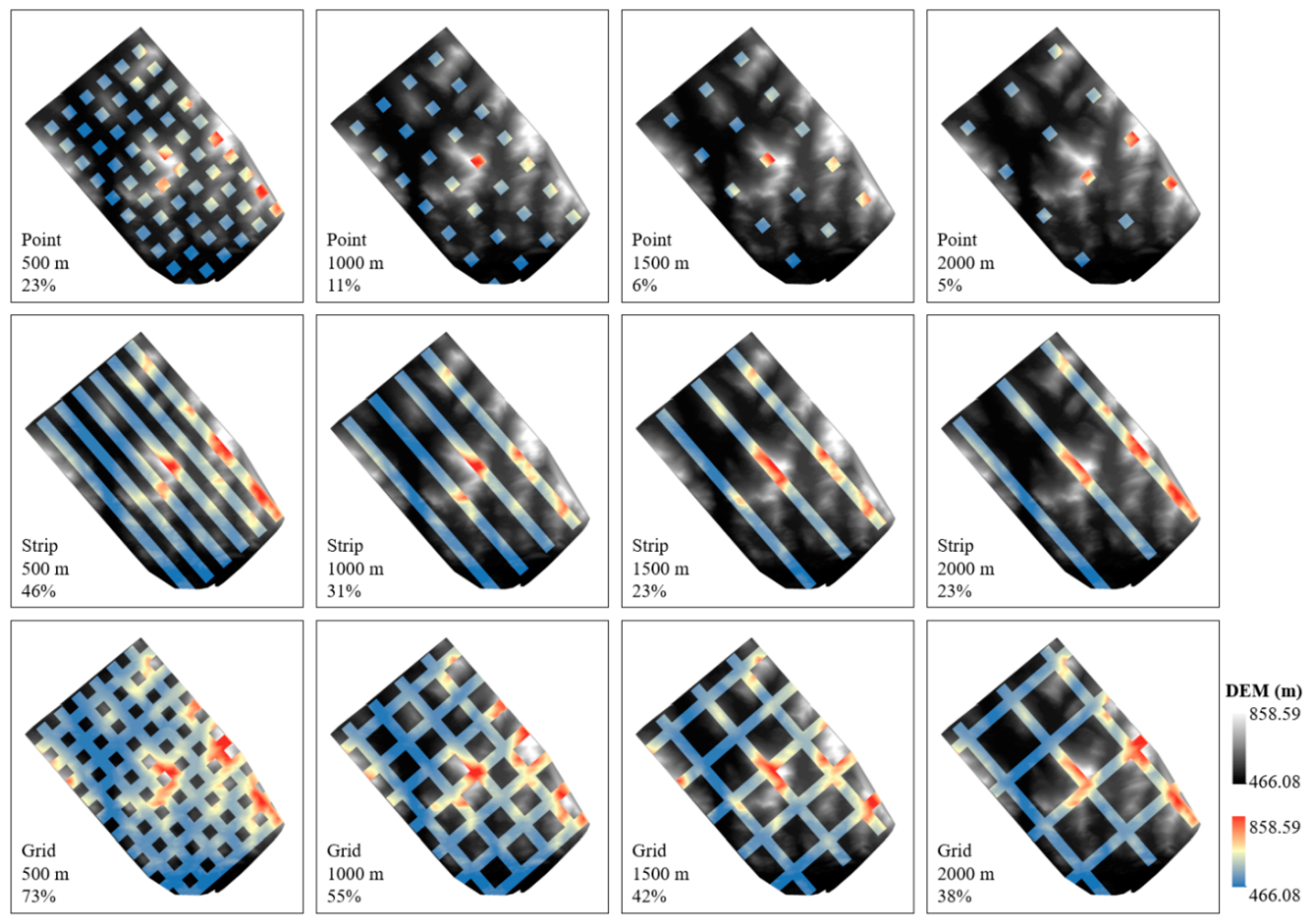
Two sampling strategies were adopted in this study: Systematic and classification-based sampling. In systematic sampling, combinations of 3 sampling patterns (point, strip, and grid) and 4 sampling intervals (500 m, 1000 m, 1500 m, and 2000 m) were applied to acquire 12 systematic lidar samples (Figure 4). A northwest-southeast alignment was applied to be consistent with the airplane flight path used during the lidar acquisition. The classification-based sampling used the same sampling pattern and amount of data as the best performing systematic sampling strategy. However, instead of using a pre-defined distance interval, the classification-based sampling selected data based on the forest type distribution within the samples.
Based on the 542 m lidar data acquisition swath width, a 500 × 500 m square area was chosen as the basic sampling unit at Huntington. However, given the smaller forest extent of our test site, for the Heiberg area, a 200 × 200 m square area was chosen as the basic sampling unit. By reducing the basic sampling unit at Heiberg, we kept the overall area percentage sampled consistent with the Huntington analysis.
2.5.4. RF Classification of Forest Type for Classification-Based Sampling
RF is a non-parametric machine learning algorithm that was implemented in this study using the “RandomForest” package [38] within the R software environment [39,40]. RF can be used for regression or classification depending on the type of variable to be estimated [41,42]. Compared with linear regression techniques, RF has a lower bias and avoids overfitting [43,44,45,46,47]. RF grows many trees to vote for a result, which makes it insensitive to outliers and noise [44,45]. For each tree, approximately two-thirds of the original data was randomly chosen to build the tree, and the remaining data were used for estimating out-of-bag error and calculating variable importance. In this study, RF was applied to develop a forest type classification map using forest inventory plots as reference data and Landsat derived variables as predictors. The forest type classification map identified 3 classes: Hardwood, mixed, and softwood forests. Default RF parameters were applied: 500 for ntree, square foot of the total predictors for mtry, and 1 for node size.
2.5.5. Chi-Square Test for Selecting Classification-Based Samples
For the classification-based sampling, the sampling pattern and percentage of the sampled area were chosen according to the performance of different systematic sampling plans. Our testing demonstrated that there was a need to identify a sample that represented the overall distribution of forests within the study site. There are multiple approaches that can be used to explore the relationship between a sample and the population. The chi-square goodness of fit test is used to determine whether an observed categorical variable frequency distribution differs from an expected distribution.
where is the observed frequency, is the expected frequency, N is the total number of observations, and is the percentage of type i in the expected distribution. The similarity between observed and expected distribution can be inferred from the value. Smaller values indicate more similar distributions. In this study, forest type distribution from the sampled area was our observed distribution and forest type distribution from the whole study area was our expected distribution. We divided the study site into multiple non-overlapping strips. Using this method, we calculated values between the whole study area and each strip based on forest type distribution. Smaller values correspond to strips with forest type composition that was closer to the whole study site.
2.5.6. Accuracy Assessment for Second Stage Regression Models
We used 10-fold cross-validation to assess the quality of AGB estimation of the first stage regression model. The second stage regression models were assessed using model fitting R2. In addition, the Landsat AGB estimations generated from second stage regression models were compared to plot and lidar estimated AGB with accuracy reported using MAE, RMSE, and RRMSE. The plot estimated AGB was calculated from ground inventory plots and the lidar estimated AGB was the estimated AGB value generated by applying the first stage regression model to the whole area. Plot estimated AGB was considered the best estimate of actual AGB. Therefore, plot tested RMSE was given more importance in terms of model comparison.
where is Landsat derived AGB from second stage regression models, is plot or lidar derived AGB, m is the number of validation data points (k = 1, 2, …, m).
3. Results
3.1. Full Lidar Coverage AGB Estimation
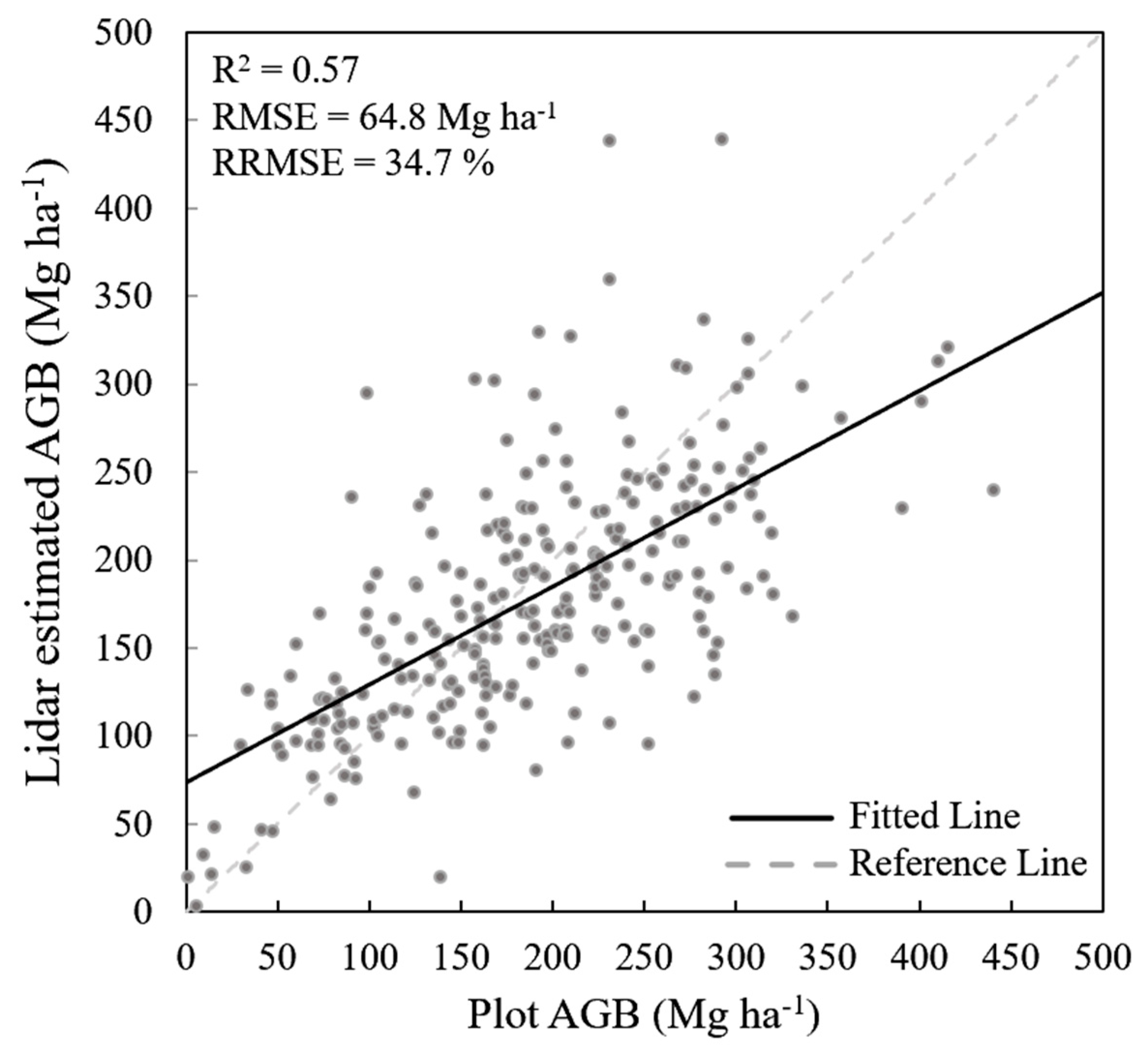
Huntington forest inventory plots and lidar derived variables were applied to establish the first stage regression model, which was validated using a 10-fold cross validation. The regression equation for the final model selected is shown in Equation (6). This equation shows the two variables selected through the forward variable selection process: ht-P90 (90th percentile of lidar point heights) and Per-first-mean (percentage of first returns above mean return height within each plot). The model has an R2 of 0.57, RMSE of 64.8 Mg ha−1, and RRMSE of 34.7% from the 10-fold cross-validation. Figure 5 shows a scatter plot illustrating the relationship between the field-based plot AGB and the lidar estimated AGB for the Huntington site.
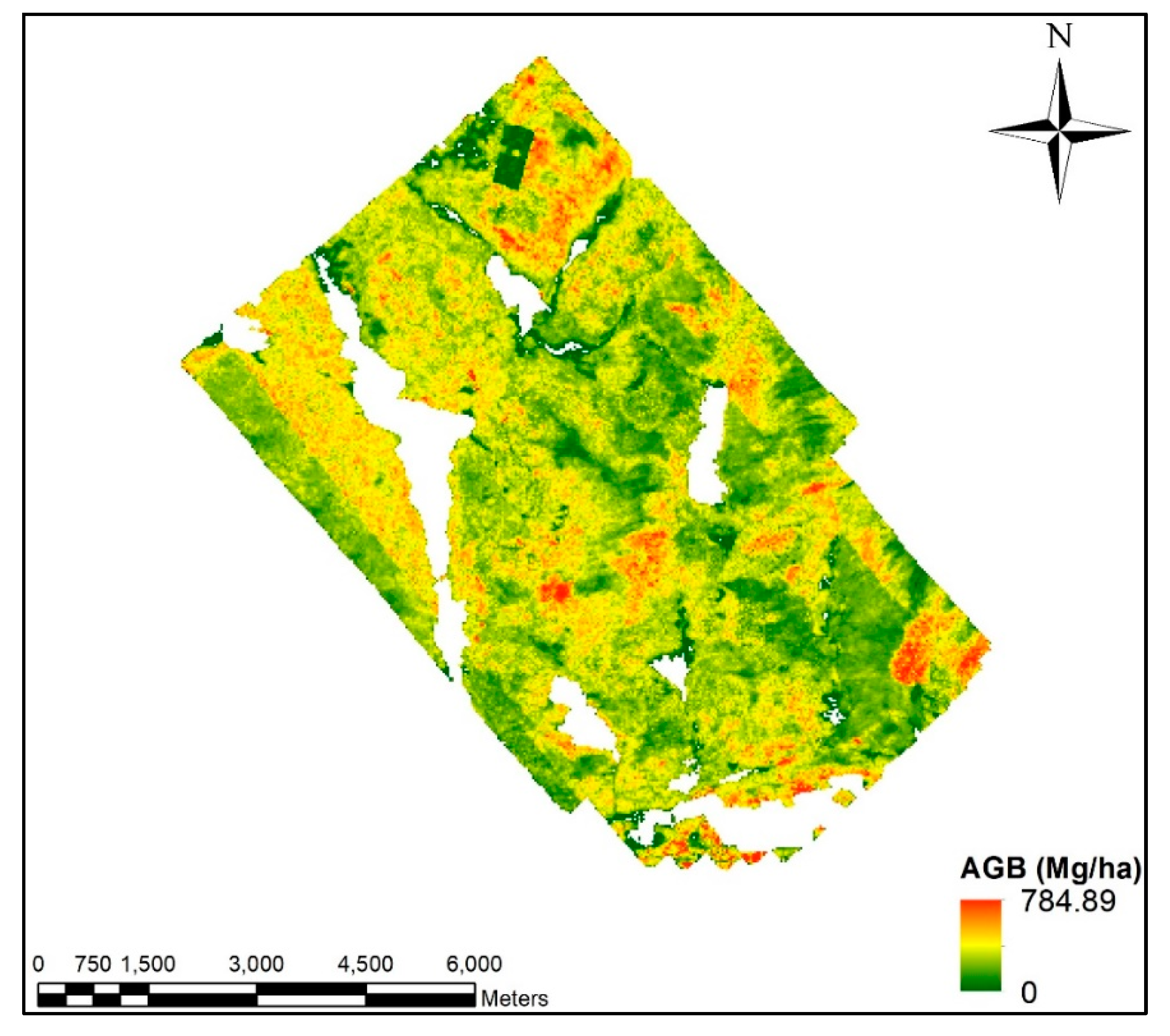
Raster layers of ht_P90 and Per_first_mean covering the whole area were created from the lidar point data. A cell size of 30 m was adopted for both raster layers to be consistent with the Landsat spatial resolution. The two raster layers were then applied in Equation (6) to generate a lidar estimated AGB map for Huntington (Figure 6). Lidar estimated AGB values at Huntington ranged from 0 to 784.89 Mg ha−1 with less than 0.3% of pixel values beyond the plot AGB maximum value of 440.3 Mg ha−1.
3.2. Systematic Sampling AGB Estimation for the Huntington Area
We used the AGB data developed from the full lidar coverage using Equation (6) as a baseline to see if the Landsat-based AGB model using lidar samples could achieve accuracies that approached that of the more expensive full lidar coverage AGB estimation. Several second stage regression models were built for each sampling strategy. The model for each sampling strategy was evaluated by looking at the model fitting R2, MAE, RMSE, and RRMSE values calculated using both the field-based plot AGB and the lidar estimated AGB as references (Table 5). The number of pixels applied for building the regression models is also summarized in Table 5.
The first stage regression model is shown in Equation (6) that used the full lidar coverage had an R2 of 0.57. Of the systematic sampling strategies, point sampling at a sample interval of 1500 m showed the highest R2 at 0.41. The point pattern generally outperformed the strip and grid patterns with higher R2 values at sample intervals of 1000 m, 1500 m, and 2000 m. None of the 12 systematic sampling strategies explored matched the RMSE and RRMSE values for AGB derived from the full lidar coverage. Using the full lidar coverage, the RMSE was 64.8 Mg ha−1 and RRMSE was 34.7% using the field-derived plot observations as a reference. Plot-based MAE, RMSE, and RRMSE for the systematic sampling strategies ranged from 67.3 to 74.6 Mg ha−1, 84.2 to 93.9 Mg ha−1 and 45.1% to 50.3%, respectively, while the lidar-based MAE, RMSE, and RRMSE ranged from 54.0 to 62.0 Mg ha−1, 70.5 to 81.1 Mg ha−1 and 40.9% to 47.0%, respectively. The strip sampling strategies had the lowest average MAE, RMSE, and RRMSE values but they also had the highest variation among different distance intervals. Strip sampling at 1500 m had the lowest plot and lidar-based MAE, RMSE, and RRMSE values among all systematic sampling strategies.
Overall, although the point sampling generally had higher R2 values, the strip sampling approach had smaller MAE, RMSE, and RRMSE values when assessed using the field-based AGB values. Strip sampling also matched the nature of airplane flight paths, which rendered it easy to adopt from a practical viewpoint. Therefore, the strip pattern was applied for further analysis.
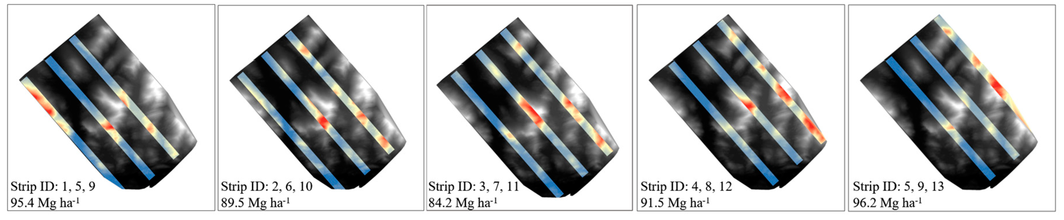
The location of the starting point for the systematic sampling determined the location of all subsequent samples. To evaluate the sensitivity of the AGB estimates to this starting point and examine the stability of systematic sampling, we tested five different starting points for the strip sampling using a 1500 m interval. Figure 7 illustrates the arrangement of the five systematic strip sampling layouts with 500 m swath width and a distance interval of 1500 m.
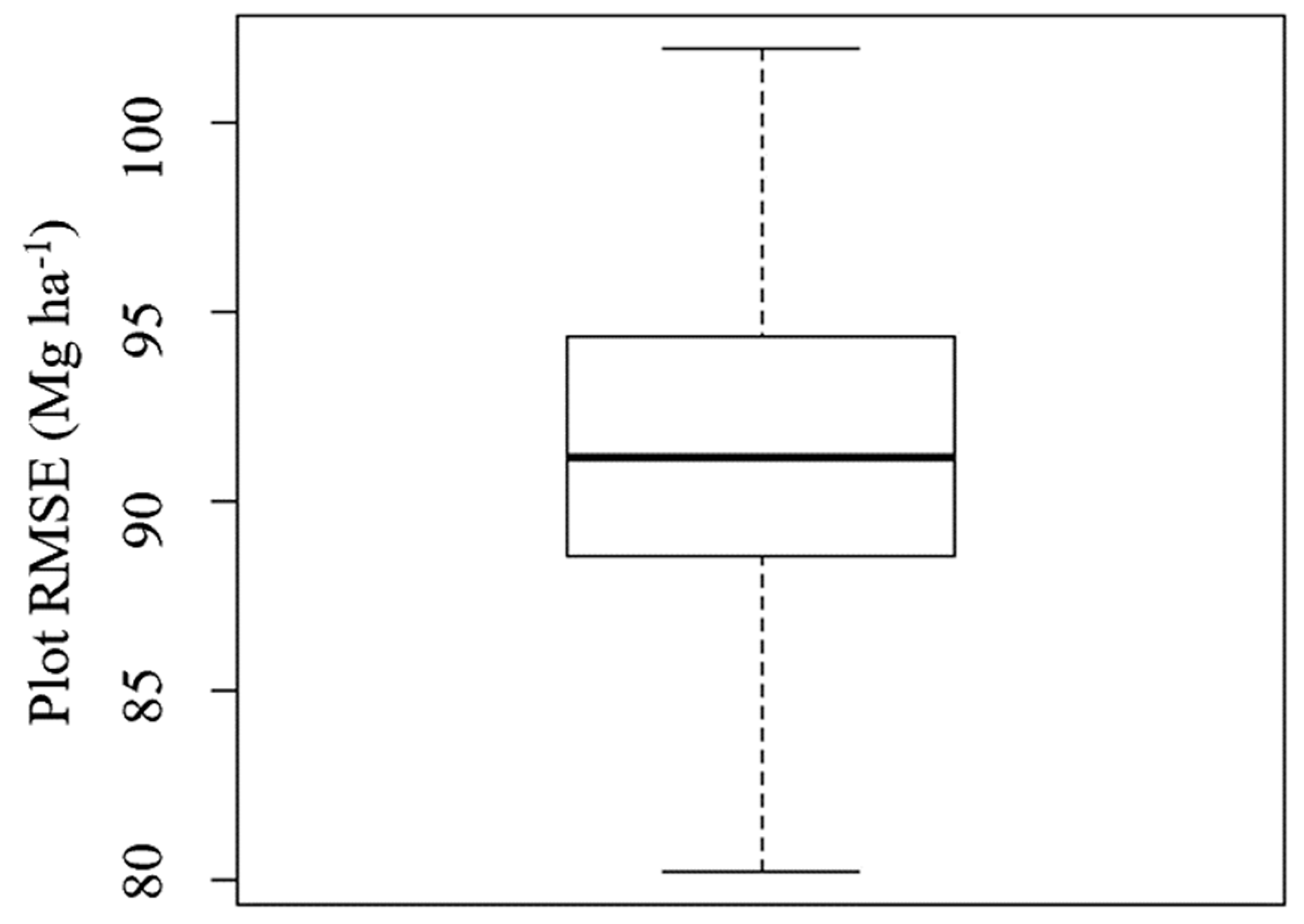
Given the variability shown in these five alternatives, we also explored the variability based on a random selection of 3 of the 13 non-overlapping strips available for this property. This led to a total of 286 combinations, with plot-based RMSE values summarized in Figure 8. The plot-based RMSE values that came from randomly selecting three strips ranged from 80.1 to 102.0 Mg ha−1.
3.3. Classification-Based Sampling AGB Estimation for the Huntington Area
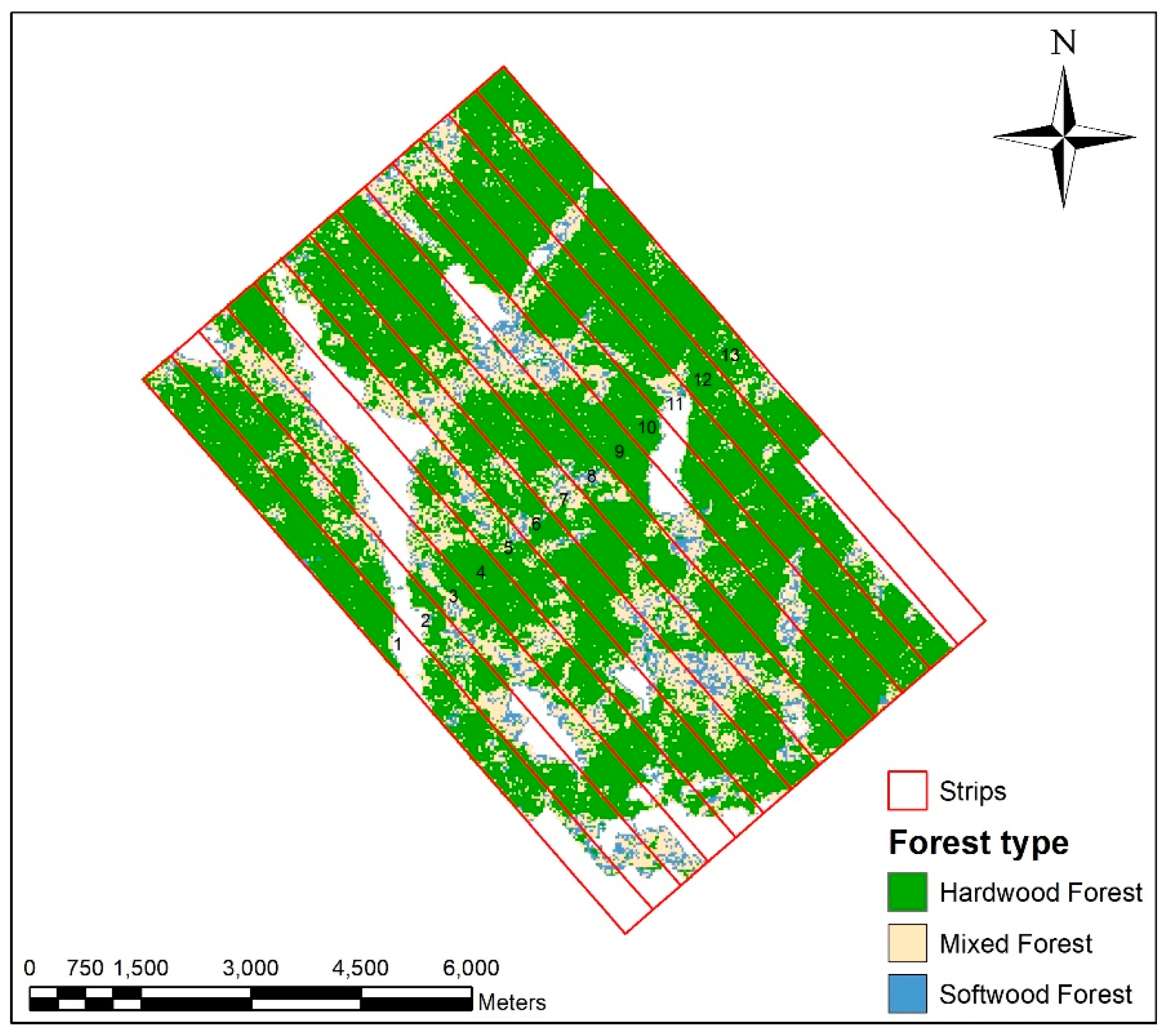
The second sampling approach explored a classification-based framework. We used a strip sampling structure at 1500 m distance intervals to select three strips from the forest type map. The forest type map was generated from the Landsat data using an RF classification with an out-of-bag (OBB) error rate of 18.9%. As with the systematic sampling, the Huntington study site was covered with 13,500 m wide non-overlapping strips. The distribution of strips and strip IDs are shown in Figure 9.
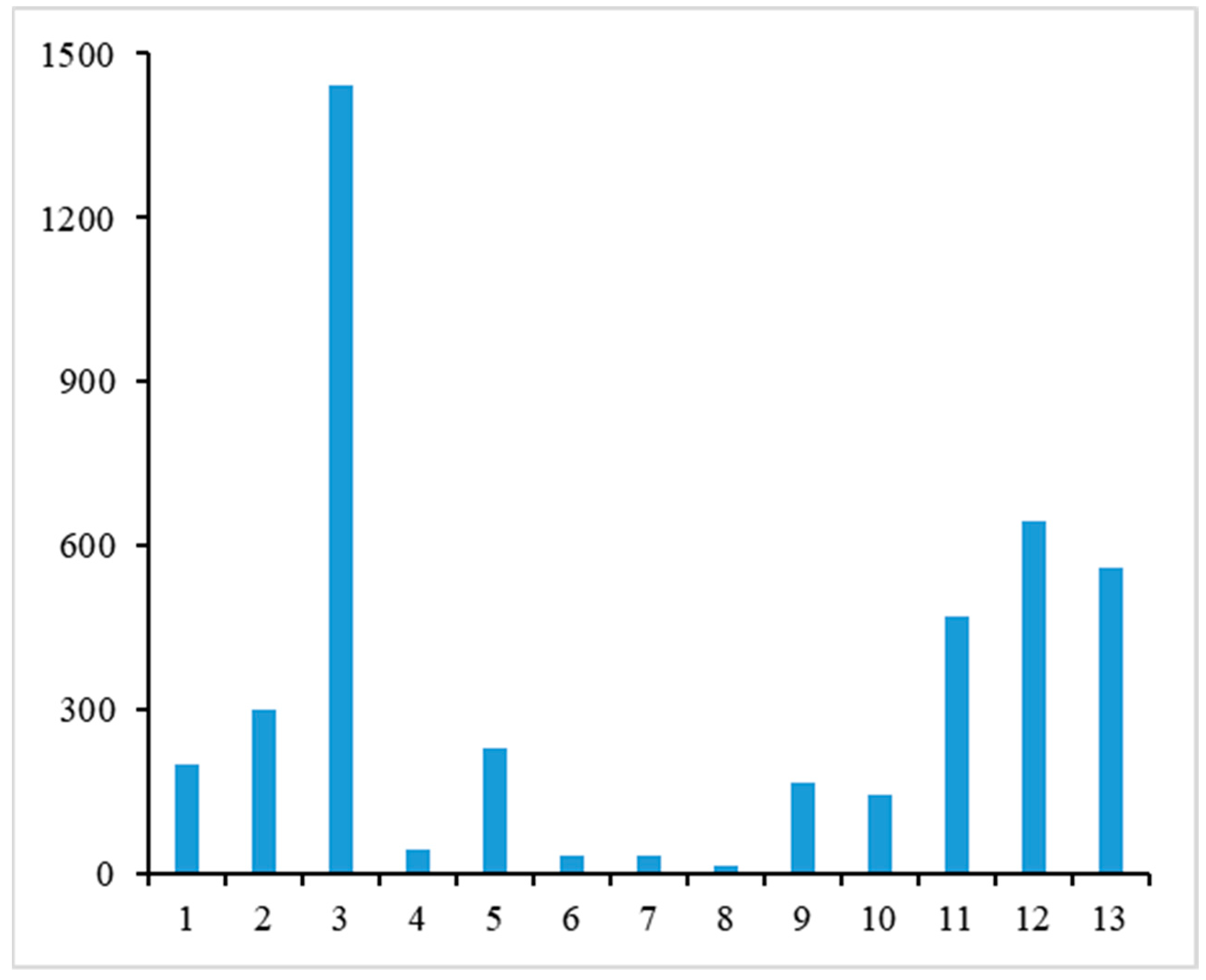
In order to select strips that best represented the entire study site, the frequency of each forest type was summarized within each strip and in the full dataset and Chi-square goodness of fit values were calculated. Strips with smaller chi-square values had a forest class distribution that was closer to the full data than strips with larger chi-square values. Strips six, seven, and eight had the smallest chi-square values (Figure 10), thus were selected to provide the classification-based lidar sample.
Lidar estimated AGB within strips six, seven, and eight were used to build a regression model with Landsat derived variables as predictors. The model results are shown in Table 6. The R2 for the classification-based sampling was generally higher than any of the 12 systematic sampling strategies and the plot and lidar tested MAE, RMSE, and RRMSE values were generally smaller. Overall, the classification-based sampling outperformed 75% of the systematic sampling strategies.
3.4. Testing Classification-Based Sampling for the Heiberg Data
A first stage regression model was built between plot AGB for all 43 Heiberg forest inventory plots and lidar derived variables following the same procedure used for the Huntington site. The regression model is shown in Equation (6). The two lidar variables identified through the forward selection process were the 95th percentile of lidar point heights (ht_P95) and the percentage of first returns above 5 m (Per-first-5 m). The model had an R2 of 0.58, RMSE of 96.0 Mg ha−1, and RRMSE of 44.7%. Raster layers for ht_P95 and Per-first-5 m were created from the Heiberg lidar points with a pixel size of 30 m. The two raster layers were applied to Equation (6) to acquire lidar estimation of AGB for Heiberg.
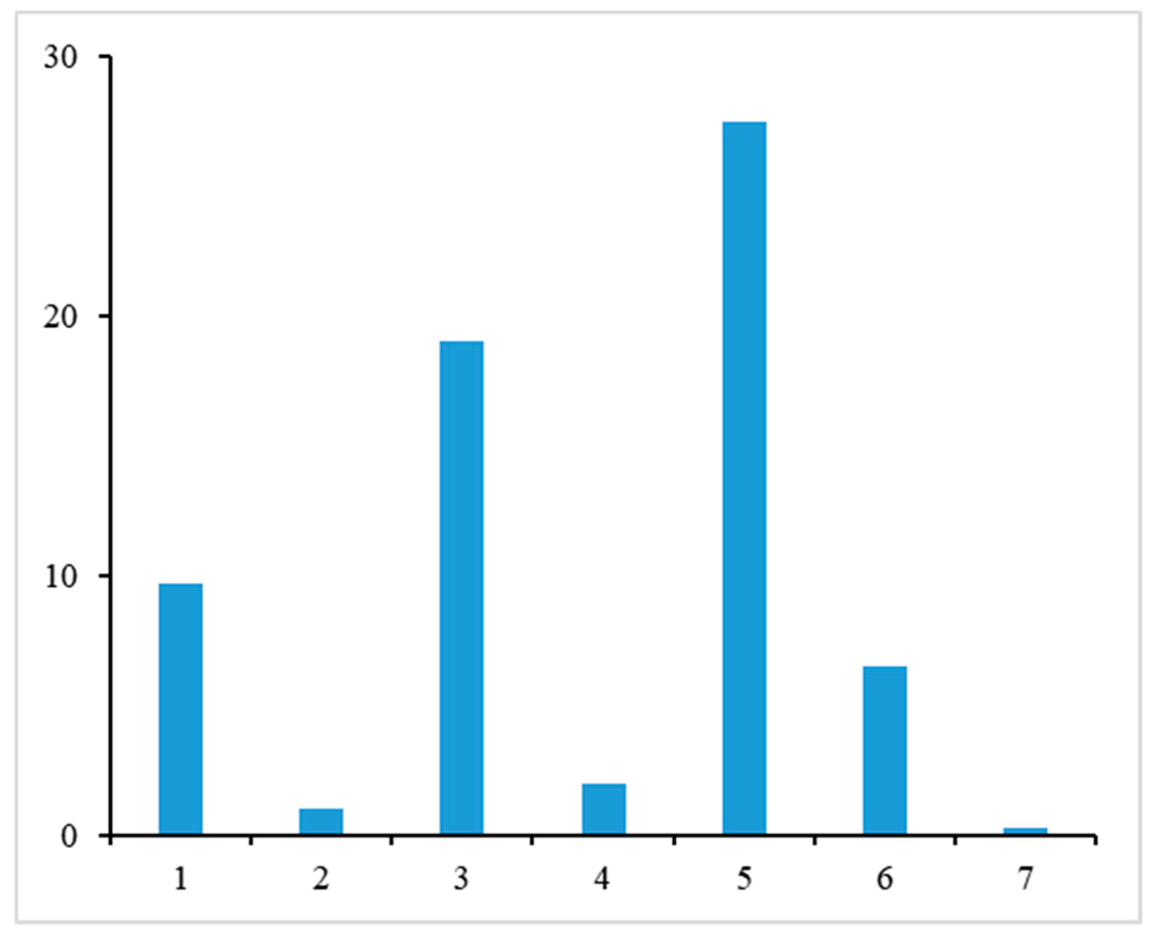
To test the transferability of the classification-based sampling method, we applied the procedure developed at Huntington to the Heiberg study area. The forest type classification map with three forest classes (hardwood, mixed, and softwood forests) was produced using RF based on forest inventory plot and Landsat data with an OBB error rate of 23.7%. The Heiberg site was smaller than the Huntington site, hence was divided into seven, 200 m wide strips along the flight path used to acquire the lidar data. Chi-square values were calculated between full data and each strip based on the distributions of forest type classes. As shown in Figure 11, strip two, four, and seven had the smallest chi-square values hence lidar estimated AGB values in those strips were used as the dependent variable and Landsat variables were used as predictors in the regression model.
The regression model built using the sample strips was then applied to the Landsat data covering the Heiberg study area to acquire AGB estimates. Landsat AGB estimates were tested using plot and lidar estimated AGB values (Table 7). Compared with using full lidar coverage, the classification-based sampling decreased the R2 value from 0.58 to 0.40. Plot and lidar tested MAE, RMSE, and RRMSE values also increased.
4. Discussion
In this study, we aimed to determine if samples of lidar data could be combined with forest inventory data and Landsat imagery to produce viable wall-to-wall maps of AGB. In particular, this study aimed to assess the stability of sampling techniques in order to develop a strategy to identify lidar samples that could be fused with Landsat data to estimate AGB without substantially compromising accuracy when compared to a full lidar based model. In our study, both systematic sampling and classification-based sampling were compared to AGB derived from full lidar coverage. For our main Huntington site, when compared to having full lidar coverage, the RMSE from systematic strip sampling and classification-based sampling both had a higher RMSE (by 30% or more). One possible factor to consider in reducing this difference may relate to the proportion of data [48,49,50]. In both sampling approaches, we limited samples to under 25% of the study area. Chen et al. [51] compared the fusion of QuickBird imagery and different sized lidar samples and concluded that model performance for estimating forest canopy heights increased with lidar sampled area.
Another weakness of the sampling-based approach lies in the use of multiple regression models [52,53]. Most of our plot AGB values were in a similar range but a few had much lower values that highly influenced the multiple regression model built (Figure 5). Oversampling lower AGB plots may improve the model performance. In contrast to the AGB estimation based on full lidar coverage that used one regression model, in the sampling-based fusing approach, we used two regression models. By adding the second regression model, we introduced additional uncertainties from both Landsat data and the second statistical model [54]. In addition, the Landsat estimated AGB values from the second regression model have narrower AGB ranges compared to lidar estimated AGB values indicating the impacts of saturation. The saturation effect can be caused by the limitations of Landsat spatial, spectral, and temporal resolutions, impacts of forest type, forest structure, and topographic features [55]. The saturation effect limits the ability of Landsat to estimate high AGB levels and leads to low AGB estimation accuracy, which has been reported in other studies [4,56,57,58]. While the RMSE-based validation characterized errors associated with the regression models they do not consider errors related to forest measurement data collection or the allometric equations applied, both of which add uncertainty to the study. We minimized uncertainty associated with the allometric equations by using species-specific equations with consideration of the applicable tree DBH range. We were unable to perform uncertainty analysis on forest measurement due to the lack of repeated tree measurement and destructive AGB measurements though this is certainly a factor to consider in future studies.
Multiple studies have performed lidar sampling, with strips being the most commonly used sampling pattern among the studies [16,19,20,59]. Sampling using data strips is consistent with the nature of airplane flight planning, which makes it a good compromise between ease of use, lower cost, and accuracy. The problem faced when using systematic sampling is inconsistency. Chen and Hay [19] stated that different lidar transects would generate different results, which is consistent with our outcomes as reported in Table 5 that shows the variability in the AGB estimates from the 12 systematic sampling strategies. Systematic sampling using strips at 1500 m intervals showed better performance in terms of RMSE than the other systematic sampling strategies at Huntington study area tested with plot and lidar estimated AGB.
Systematic sampling strategy outcomes are highly connected with site conditions, modeling technique, and the use of auxiliary data [60,61]. To test the uncertainty associated with site condition variability, we explored the impact of the systematic sampling start point for strip sampling as well as the random selection of sampling strips in terms of plot-based RMSE. Our study demonstrated that even with consistency in terms of modeling technique and auxiliary data inputs, RMSE values varied substantially (Figure 7) when we used different starting points to sample three strips at a constant distance interval. RMSE values also varied substantially when we varied the location sampled through random strip selection (Figure 8). These RMSE values varied from outperforming all other systematic sampling strategies in Table 5 to be the worst sampling strategy. With such high variability of RMSE, it is hard to discern the impact of sample percentages on the AGB estimation. From a practical standpoint, it would be almost impossible to discern which systematic strategy would return a good outcome since you cannot typically explore multiple systematic sampling combinations and would not be considering sampling if the full lidar coverage was available. In our study, there was no general trend in terms of the changes in accuracy with variation in systematic sampling intervals and sampling pattern. This variability may have been linked to differences in forest condition in different regions. Gregoire et al. [62] recommended considering the AGB gradient during the sampling stage. Although Chen and Hay [19] got similar performance from N-S and E-W direction lidar samplings, this might be attributed to the complexity of the forest ecosystem in their study site, which had no general trend in any direction. If there was a general trend shown in a site, as might be the case for plantation areas, considering sampling direction is highly recommended. Our study supported prior work that demonstrated that systematic sampling is easy to apply, but the instability of the outputs suggests it has lower transferability for AGB estimation at other sites.
We applied classification-based sampling with the goal of using readily available Landsat data to select samples for acquiring lidar data that were representative of the entire study area. Land cover is an important factor in modeling AGB [63,64] and it is easy to overlook some forest types especially over large and heterogeneously distributed areas. Zheng et al. [64] showed that developing individual regression models for each forest type could improve model accuracy. In general, hardwoods have high canopy cover resulting in more horizontal expansion compared to softwood [63,65]. Selecting lidar strips based on forest type classification result could avoid over or under representation of certain forest types. The classification-based sampling outperformed 75% of the systematic sampling strategies in Huntington study area, and more importantly, provided a means to plan lidar acquisition that was lacking in the systematic sampling approach. Adopting this method to our test Heiberg area, the classification-based sampling also worked effectively, with R2 and RMSE values acquired from the classification-based sampling only moderately impacted when compared to the full lidar coverage model. The classification-based sampling method provides a means to substantially reduce lidar acquisition without a major compromise in accuracy while providing a preprocessing step to guide application in new study areas. The need to perform the classification does require additional analysis; however, the random nature of systematic sampling can lead to substantial, and unknown a priori, sample variability that potentially decreases transferability of this approach.
5. Conclusions
The framework in this study provides an approach to obtain wall-to-wall estimates of AGB by merging lidar samples with Landsat imagery and forest inventory data. We focused on AGB estimation accuracy based on systematic and classification-based lidar sampling strategies. While systematic lidar sampling can achieve promising AGB estimates and is easy to implement, there was high model outcome variability among systematic sampling strategies. Moreover, the results attained from systematic sampling strategies were highly dependent on site condition, which provides challenges in planning lidar acquisitions. Classification-based lidar sampling provides a planning framework that is more readily transferable to new sites by guiding the selection of lidar samples representative of the study site. The fusion of lidar samples and Landsat data had lower accuracies in AGB estimation compared with full lidar coverage, which can be exacerbated by the uncertainties introduced by the addition of Landsat data and the use of a second regression model. This study performed a methodical comparison of systematic and classification-based lidar sampling approaches to support AGB estimation. We propose using forest type classification as a means to guide lidar sampling selection within this field. We anticipate the results of this study could facilitate cost-effective lidar data collection for use in future studies.
Author Contributions
Conceptualization, S.L.; Methodology, S.L. and L.J.Q.; Validation, S.L. and L.J.Q.; Writing, S.L.; Review and Editing, S.L., L.J.Q. and J.I.
Funding
This research received no external funding.
Conflicts of Interest
The authors declare no conflict of interest.
References
- Matasci, G.; Hermosilla, T.; Wulder, M.A.; White, J.C.; Coops, N.C.; Hobart, G.W.; Zald, H.S. Large-area mapping of Canadian boreal forest cover, height, biomass and other structural attributes using Landsat composites and lidar plots. Remote Sens. Environ. 2018, 209, 90–106. [Google Scholar] [CrossRef]
- Chen, Q.; Laurin, G.V.; Battles, J.J.; Saah, D. Integration of airborne lidar and vegetation types derived from aerial photography for mapping aboveground live biomass. Remote Sens. Environ. 2012, 121, 108–117. [Google Scholar] [CrossRef]
- Maltamo, M.; Eerikäinen, K.; Packalén, P.; Hyyppä, J. Estimation of stem volume using laser scanning-based canopy height metrics. Forestry 2006, 79, 217–229. [Google Scholar] [CrossRef] [Green Version]
- Lu, D.; Chen, Q.; Wang, G.; Moran, E.; Batistella, M.; Zhang, M.; Vaglio Laurin, G.; Saah, D. Aboveground forest biomass estimation with Landsat and LiDAR data and uncertainty analysis of the estimates. Int. J. For. Res. 2012, 2012, 1–16. [Google Scholar] [CrossRef]
- Zhang, Y.; Liang, S.; Sun, G. Forest biomass mapping of northeastern China using GLAS and MODIS data. IEEE J. Sel. Top. Appl. Earth Obs. Remote Sens. 2014, 7, 140–152. [Google Scholar] [CrossRef]
- Baghdadi, N.; Le Maire, G.; Bailly, J.S.; Osé, K.; Nouvellon, Y.; Zribi, M.; Lemos, C.; Hakamada, R. Evaluation of ALOS/PALSAR L-band data for the estimation of eucalyptus plantations aboveground biomass in Brazil. IEEE J. Sel. Top. Appl. Earth Obs. Remote Sens. 2015, 8, 3802–3811. [Google Scholar] [CrossRef]
- Knapp, N.; Huth, A.; Kugler, F.; Papathanassiou, K.; Condit, R.; Hubbell, S.P.; Fischer, R. Model-assisted estimation of tropical forest biomass change: A comparison of approaches. Remote Sens. 2018, 10, 731. [Google Scholar] [CrossRef]
- Mitchard, E.T.; Saatchi, S.S.; Woodhouse, I.H.; Nangendo, G.; Ribeiro, N.; Williams, M.; Ryan, C.M.; Lewis, S.L.; Feldpausch, T.; Meir, P. Using satellite radar backscatter to predict above-ground woody biomass: A consistent relationship across four different African landscapes. Geophys. Res. Lett. 2009, 36, L23401. [Google Scholar] [CrossRef]
- Hajj, M.; Baghdadi, N.; Fayad, I.; Vieilledent, G.; Bailly, J.-S.; Minh, D. Interest of integrating spaceborne LiDAR data to improve the estimation of biomass in high biomass forested areas. Remote Sens. 2017, 9, 213. [Google Scholar] [CrossRef]
- Kelly, M.; Di Tommaso, S. Mapping forests with Lidar provides flexible, accurate data with many uses. Calif. Agric. 2015, 69, 14–20. [Google Scholar] [CrossRef]
- Erdody, T.L.; Moskal, L.M. Fusion of LiDAR and imagery for estimating forest canopy fuels. Remote Sens. Environ. 2010, 114, 725–737. [Google Scholar] [CrossRef]
- Ediriweera, S.; Pathirana, S.; Danaher, T.; Nichols, D. Estimating above-ground biomass by fusion of LiDAR and multispectral data in subtropical woody plant communities in topographically complex terrain in North-Eastern Australia. J. For. Res. 2014, 25, 761–771. [Google Scholar] [CrossRef]
- Ørka, H.O.; Wulder, M.A.; Gobakken, T.; Næsset, E. Subalpine zone delineation using LiDAR and Landsat imagery. Remote Sens. Environ. 2012, 119, 11–20. [Google Scholar] [CrossRef]
- Ene, L.T.; Næsset, E.; Gobakken, T.; Mauya, E.W.; Bollandsås, O.M.; Gregoire, T.G.; Ståhl, G.; Zahabu, E. Large-scale estimation of aboveground biomass in miombo woodlands using airborne laser scanning and national forest inventory data. Remote Sens. Environ. 2016, 186, 626–636. [Google Scholar] [CrossRef]
- Næsset, E.; Gobakken, T.; Nelson, R. Sampling and mapping forest volume and biomass using airborne LIDARs. In Proceedings of the 8th Annual Forest Inventory and Analysis Symposium, Monterey, CA, USA, 16–19 October 2006; McRoberts, R.E., Reams, G.A., Van Deusen, P.C., McWilliams, W.H., Eds.; Gen. Tech. Report WO-79. United States Department of Agriculture, Forest Service: Washington, DC, USA, 2009; Volume 79, pp. 297–301. [Google Scholar]
- Hudak, A.T.; Lefsky, M.A.; Cohen, W.B.; Berterretche, M. Integration of lidar and Landsat ETM+ data for estimating and mapping forest canopy height. Remote Sens. Environ. 2002, 82, 397–416. [Google Scholar] [CrossRef] [Green Version]
- Boudreau, J.; Nelson, R.; Margolis, H.; Beaudoin, A.; Guindon, L.; Kimes, D. Regional aboveground forest biomass using airborne and spaceborne LiDAR in Québec. Remote Sens. Environ. 2008, 112, 3876–3890. [Google Scholar] [CrossRef]
- Holmgren, J. Prediction of tree height, basal area and stem volume in forest stands using airborne laser scanning. Scand. J. For. Res. 2004, 19, 543–553. [Google Scholar] [CrossRef]
- Chen, G.; Hay, G.J. An airborne lidar sampling strategy to model forest canopy height from Quickbird imagery and GEOBIA. Remote Sens. Environ. 2011, 115, 1532–1542. [Google Scholar] [CrossRef]
- Tsui, O.W.; Coops, N.C.; Wulder, M.A.; Marshall, P.L. Integrating airborne LiDAR and space-borne radar via multivariate kriging to estimate above-ground biomass. Remote Sens. Environ. 2013, 139, 340–352. [Google Scholar] [CrossRef]
- Shepard, J.P.; Mitchell, M.J.; Scott, T.J.; Zhang, Y.M.; Raynal, D.J. Measurements of wet and dry deposition in a Northern Hardwood forest. Water Air Soil Pollut. 1989, 48, 225–238. [Google Scholar] [CrossRef]
- Multi-Resolution Land Characteristics Consortium. Available online: https://www.mrlc.gov/ (accessed on 21 July 2019).
- Jenkins, J.C.; Chojnacky, D.C.; Heath, L.S.; Birdsey, R.A. National-scale biomass estimators for United States tree species. For. Sci. 2003, 49, 12–35. [Google Scholar]
- UNECE/FAO. Forest Resources of Europe, CIS, North America, Australia, Japan and New Zealand (Industrialized Temperate/Boreal Countries): UN-ECE/FAO Contribution to the Global Forest Resources Assessment 2000; United Nations: New York, NY, USA; Geneva, Switzerland, 2000. [Google Scholar]
- Software for Processing Point Clouds and Images. Available online: https://www.terrasolid.com/home.php (accessed on 15 July 2017).
- FUSION Version Check. Available online: http://forsys.cfr.washington.edu/fusion/fusionlatest.html (accessed on 8 April 2018).
- McGaughey, R.J. FUSION/LDV: Software for LIDAR Data Analysis and Visualization; United States Department of Agriculture, Forest Service, Pacific Northwest Research Station: Seattle, WA, USA, 2019.
- EarthExplorer. Available online: https://earthexplorer.usgs.gov/ (accessed on 9 March 2018).
- Harris Geospatial Solutions. Available online: http://www.harrisgeospatial.com/Home.aspx (accessed on 9 March 2018).
- Bacour, C.; Bréon, F.M.; Maignan, F. Normalization of the directional effects in NOAA–AVHRR reflectance measurements for an improved monitoring of vegetation cycles. Remote Sens. Environ. 2006, 102, 402–413. [Google Scholar] [CrossRef]
- Jordan, C.F. Derivation of leaf-area index from quality of light on the forest floor. Ecology 1969, 50, 663–666. [Google Scholar] [CrossRef]
- Tucker, C.J. Red and photographic infrared linear combinations for monitoring vegetation. Remote Sens. Environ. 1979, 8, 127–150. [Google Scholar] [CrossRef] [Green Version]
- Huete, A.R. A soil-adjusted vegetation index (SAVI). Remote Sens. Environ. 1988, 25, 295–309. [Google Scholar] [CrossRef]
- Qi, J.; Chehbouni, A.; Huete, A.; Kerr, Y.; Sorooshian, S. A modified soil adjusted vegetation index. Remote Sens. Environ. 1994, 48, 119–126. [Google Scholar] [CrossRef]
- Li, M.; Im, J.; Beier, C. Machine learning approaches for forest classification and change analysis using multi-temporal Landsat TM images over Huntington Wildlife Forest. GISci. Remote Sens. 2013, 50, 361–384. [Google Scholar] [CrossRef]
- Ali, A.; Lin, S.L.; He, J.K.; Kong, F.M.; Yu, J.H.; Jiang, H.S. Tree crown complementarity links positive functional diversity and aboveground biomass along large-scale ecological gradients in tropical forests. Sci. Total Environ. 2019, 656, 45–54. [Google Scholar] [CrossRef] [PubMed]
- Van Vinh, T.; Marchand, C.; Linh, T.V.K.; Vinh, D.D.; Allenbach, M. Allometric models to estimate above-ground biomass and carbon stocks in Rhizophora apiculata tropical managed mangrove forests (Southern Vietnam). For. Ecol. Manag. 2019, 434, 131–141. [Google Scholar] [CrossRef]
- Liaw, A.; Wiener, M. Classification and regression by randomForest. R News 2002, 2, 18–22. [Google Scholar]
- Richardson, H.J.; Hill, D.J.; Denesiuk, D.R.; Fraser, L.H. A comparison of geographic datasets and field measurements to model soil carbon using random forests and stepwise regressions (British Columbia, Canada). GISci. Remote Sens. 2017, 54, 573–591. [Google Scholar] [CrossRef]
- R Project. Available online: http://www.R-project.org (accessed on 17 March 2018).
- Sonobe, R.; Yamaya, Y.; Tani, H.; Wang, X.; Kobayashi, N.; Mochizuki, K. Assessing the suitability of data from Sentinel-1A and 2A for crop classification. GISci. Remote Sens. 2017, 54, 918–938. [Google Scholar] [CrossRef]
- Zhang, C.; Smith, M.; Fang, C. Evaluation of Goddard’s LiDAR, hyperspectral, and thermal data products for mapping urban land-cover types. GISci. Remote Sens. 2018, 55, 90–109. [Google Scholar] [CrossRef]
- Boisvenue, C.; Smiley, B.P.; White, J.C.; Kurz, W.A.; Wulder, M.A. Integration of Landsat time series and field plots for forest productivity estimates in decision support models. For. Ecol. Manag. 2016, 376, 284–297. [Google Scholar] [CrossRef]
- Ghosh, S.M.; Behera, M.D. Aboveground biomass estimation using multi-sensor data synergy and machine learning algorithms in a dense tropical forest. Appl. Geogr. 2018, 96, 29–40. [Google Scholar] [CrossRef]
- Gleason, C.J.; Im, J. Forest biomass estimation from airborne LiDAR data using machine learning approaches. Remote Sens. Environ. 2012, 125, 80–91. [Google Scholar] [CrossRef]
- Tian, X.; Yan, M.; van der Tol, C.; Li, Z.; Su, Z.; Chen, E.; Li, X.; Li, L.; Wang, X.; Pan, X.; et al. Modeling forest above-ground biomass dynamics using multi-source data and incorporated models: A case study over the qilian mountains. Agric. For. Meteorol. 2017, 246, 1–14. [Google Scholar] [CrossRef]
- Georganos, S.; Grippa, T.; Vanhuysse, S.; Lennert, M.; Shimoni, M.; Kalogirou, S.; Wolff, E. Less is more: Optimizing classification performance through feature selection in a very-high-resolution remote sensing object-based urban application. GISci. Remote Sens. 2018, 55, 221–242. [Google Scholar] [CrossRef]
- Hopkinson, C.; Chasmer, L.; Gynan, C.; Mahoney, C.; Sitar, M. Multisensor and multispectral lidar characterization and classification of a forest environment. Can. J. Remote Sens. 2016, 42, 501–520. [Google Scholar] [CrossRef]
- Luo, S.; Chen, J.M.; Wang, C.; Xi, X.; Zeng, H.; Peng, D.; Li, D. Effects of LiDAR point density, sampling size and height threshold on estimation accuracy of crop biophysical parameters. Opt. Express 2016, 24, 11578–11593. [Google Scholar] [CrossRef]
- Saarela, S.; Grafström, A.; Ståhl, G.; Kangas, A.; Holopainen, M.; Tuominen, S.; Nordkvist, K.; Hyyppä, J. Model-assisted estimation of growing stock volume using different combinations of LiDAR and Landsat data as auxiliary information. Remote Sens. Environ. 2015, 158, 431–440. [Google Scholar] [CrossRef]
- Chen, G.; Hay, G.J.; St-Onge, B. A GEOBIA framework to estimate forest parameters from lidar transects, Quickbird imagery and machine learning: A case study in Quebec, Canada. Int. J. Appl. Earth Obs. Geoinf. 2012, 15, 28–37. [Google Scholar] [CrossRef]
- Feng, Y.; Lu, D.; Chen, Q.; Keller, M.; Moran, E.; dos-Santos, M.N.; Bolfe, E.L.; Batistella, M. Examining effective use of data sources and modeling algorithms for improving biomass estimation in a moist tropical forest of the Brazilian Amazon. Int. J. Digit. Earth 2017, 10, 996–1016. [Google Scholar] [CrossRef]
- Li, W.; Niu, Z.; Liang, X.; Li, Z.; Huang, N.; Gao, S.; Wang, C.; Muhammad, S. Geostatistical modeling using LiDAR-derived prior knowledge with SPOT-6 data to estimate temperate forest canopy cover and above-ground biomass via stratified random sampling. Int. J. Appl. Earth Obs. Geoinf. 2015, 41, 88–98. [Google Scholar] [CrossRef]
- Skowronski, N.S.; Clark, K.L.; Gallagher, M.; Birdsey, R.A.; Hom, J.L. Airborne laser scanner-assisted estimation of aboveground biomass change in a temperate oak–pine forest. Remote Sens. Environ. 2014, 151, 166–174. [Google Scholar] [CrossRef]
- Zhao, P.; Lu, D.; Wang, G.; Wu, C.; Huang, Y.; Yu, S. Examining spectral reflectance saturation in Landsat imagery and corresponding solutions to improve forest aboveground biomass estimation. Remote Sens. 2016, 8, 469. [Google Scholar] [CrossRef]
- Nichol, J.E.; Sarker, M.L.R. Improved biomass estimation using the texture parameters of two high-resolution optical sensors. IEEE Trans. Geosci. Remote Sens. 2010, 49, 930–948. [Google Scholar] [CrossRef]
- Shen, W.; Li, M.; Huang, C.; Tao, X.; Wei, A. Annual forest aboveground biomass changes mapped using ICESat/GLAS measurements, historical inventory data, and time-series optical and radar imagery for Guangdong province, China. Agric. For. Meteorol. 2018, 259, 23–38. [Google Scholar] [CrossRef] [Green Version]
- Vaglio Laurin, G.; Pirotti, F.; Callegari, M.; Chen, Q.; Cuozzo, G.; Lingua, E.; Notarnicola, C.; Papale, D. Potential of ALOS2 and NDVI to estimate forest above-ground biomass, and comparison with lidar-derived estimates. Remote Sens. 2017, 9, 18. [Google Scholar] [CrossRef]
- Hilker, T.; Wulder, M.A.; Coops, N.C. Update of forest inventory data with lidar and high spatial resolution satellite imagery. Can. J. Remote Sens. 2008, 34, 5–12. [Google Scholar] [CrossRef]
- Almeida, D.R.A.d.; Stark, S.C.; Shao, G.; Schietti, J.; Nelson, B.W.; Silva, C.A.; Gorgens, E.B.; Valbuena, R.; Papa, D.d.A.; Brancalion, P.H.S. Optimizing the remote detection of tropical rainforest structure with airborne lidar: Leaf area profile sensitivity to pulse density and spatial sampling. Remote Sens. 2019, 11, 92. [Google Scholar] [CrossRef]
- Cao, L.; Coops, N.C.; Sun, Y.; Ruan, H.; Wang, G.; Dai, J.; She, G. Estimating canopy structure and biomass in bamboo forests using airborne LiDAR data. ISPRS J. Photogramm. Remote Sens. 2019, 148, 114–129. [Google Scholar] [CrossRef]
- Gregoire, T.G.; Ståhl, G.; Næsset, E.; Gobakken, T.; Nelson, R.; Holm, S. Model-assisted estimation of biomass in a LiDAR sample survey in Hedmark County, Norway. Can. J. For. Res. 2010, 41, 83–95. [Google Scholar] [CrossRef]
- Zheng, D.; Rademacher, J.; Chen, J.; Crow, T.; Bresee, M.; Le Moine, J.; Ryu, S.-R. Estimating aboveground biomass using Landsat 7 ETM+ data across a managed landscape in northern Wisconsin, USA. Remote Sens. Environ. 2004, 93, 402–411. [Google Scholar] [CrossRef]
- Zheng, G.; Chen, J.M.; Tian, Q.J.; Ju, W.M.; Xia, X.Q. Combining remote sensing imagery and forest age inventory for biomass mapping. J. Environ. Manag. 2007, 85, 616–623. [Google Scholar] [CrossRef] [PubMed]
- Yang, Y.; Yanai, R.D.; See, C.R.; Arthur, M.A. Sampling effort and uncertainty in leaf litterfall mass and nutrient flux in northern hardwood forests. Ecosphere 2017, 8, e01999. [Google Scholar] [CrossRef]
Figure 1.
Location of Huntington Wildlife Forest in New York State. The figure shows the distribution of 270 forest inventory plots overlaid on land cover from the National Land Cover Database 2016 [22].
Figure 1.
Location of Huntington Wildlife Forest in New York State. The figure shows the distribution of 270 forest inventory plots overlaid on land cover from the National Land Cover Database 2016 [22].

Figure 2.
Location of Heiberg Memorial Forest in New York State. The figure shows the distribution of 43 forest inventory plots overlaid on land cover from the National Land Cover Database 2016 [22].
Figure 2.
Location of Heiberg Memorial Forest in New York State. The figure shows the distribution of 43 forest inventory plots overlaid on land cover from the National Land Cover Database 2016 [22].

Figure 3.
Flowchart of the research process including data, sampling strategies, methods, and results.
Figure 3.
Flowchart of the research process including data, sampling strategies, methods, and results.

Figure 4.
Distribution of lidar samples generated from twelve systematic lidar sampling strategies. Each sampling strategy had a unique combination of sampling pattern, distance interval, and the percentage of the sampled area as indicated in the lower left corner of each panel. Sampled area is shown in color on top of the greyscale digital elevation model.

Figure 5.
Scatter plot between plot and lidar estimated AGB at the Huntington Wildlife Forest.

Figure 6.
Lidar estimated AGB distribution map calculated using Equation (6) and the lidar derived ht-P90 and Per_first_mean raster layers. Lidar estimated AGB values at Huntington ranged from 0 tp 784.89 Mg ha−1. Water areas were masked out.
Figure 6.
Lidar estimated AGB distribution map calculated using Equation (6) and the lidar derived ht-P90 and Per_first_mean raster layers. Lidar estimated AGB values at Huntington ranged from 0 tp 784.89 Mg ha−1. Water areas were masked out.

Figure 7.
Possible outcomes using strip sampling pattern at a 1500 m distance interval. The sampled strip ID and plot based root mean square error (RMSE) values are listed in the lower left corner of each part of the figure.
Figure 7.
Possible outcomes using strip sampling pattern at a 1500 m distance interval. The sampled strip ID and plot based root mean square error (RMSE) values are listed in the lower left corner of each part of the figure.

Figure 8.
Boxplot summarizing plot-based RMSE values from 286 possible sampling outcomes that were generated by randomly selecting 3 of the 13 strips on the Huntington site.
Figure 8.
Boxplot summarizing plot-based RMSE values from 286 possible sampling outcomes that were generated by randomly selecting 3 of the 13 strips on the Huntington site.

Figure 9.
Random forest (RF) forest type classification of the Huntington site. The classification used Landsat derived variables as predictors and plot inventory information as a reference. Strips (with ID labeled) used for sampling are overlaid on top of the classification map.
Figure 9.
Random forest (RF) forest type classification of the Huntington site. The classification used Landsat derived variables as predictors and plot inventory information as a reference. Strips (with ID labeled) used for sampling are overlaid on top of the classification map.

Figure 10.
Chi-square values between the full coverage and each strip in terms of forest type frequency. The X axis is strip ID and the Y axis is chi-square goodness of fit value.
Figure 10.
Chi-square values between the full coverage and each strip in terms of forest type frequency. The X axis is strip ID and the Y axis is chi-square goodness of fit value.

Figure 11.
Chi-square values between all data and each strip. X axis is strip name and the Y axis is chi-square value.
Figure 11.
Chi-square values between all data and each strip. X axis is strip name and the Y axis is chi-square value.


Table 1.
Plot level aboveground biomass (AGB) descriptive statistics for all plots and plots grouped by forest type (hardwood, softwood, and mixed) in Huntington and Heiberg forests (units: Mg ha−1).
Table 1.
Plot level aboveground biomass (AGB) descriptive statistics for all plots and plots grouped by forest type (hardwood, softwood, and mixed) in Huntington and Heiberg forests (units: Mg ha−1).
| Study Area | Forest Type | Plot Count | AGB (Mg ha−1) | ||||
|---|---|---|---|---|---|---|---|
| Mean | Median | Standard Deviation | Min | Max | |||
| Huntington | Total | 270 | 186.6 | 186.3 | 82.5 | 0.9 | 440.3 |
| Hardwood | 194 | 182.3 | 184.5 | 81.8 | 0.9 | 440.3 | |
| Mixed | 60 | 211.9 | 208.7 | 73.9 | 68.8 | 390.7 | |
| Softwood | 16 | 144.3 | 133.9 | 98.8 | 9.1 | 314.7 | |
| Heiberg | Total | 43 | 212.6 | 215.9 | 98.4 | 2.0 | 375.8 |
| Hardwood | 31 | 220.8 | 249.7 | 98.5 | 2.0 | 375.8 | |
| Mixed | 9 | 220.3 | 249.0 | 88.6 | 76.4 | 323.9 | |
| Softwood | 3 | 104.9 | 59.5 | 86.9 | 50.1 | 205.1 | |
Table 2.
ALS60 system settings and raw laser statistics of the lidar data collection for Huntington and Heiberg forests.
Table 2.
ALS60 system settings and raw laser statistics of the lidar data collection for Huntington and Heiberg forests.
| Study Site | Huntington | Heiberg |
|---|---|---|
| Scan field of view (FOV) | 24° | 28° |
| Outgoing pulse width | 4 ns | 4 ns |
| Flying altitude | 540 m | 487 m |
| Swath width | ~542 m | ~554 m |
| Average point density | >10 pts/m2 | >7 pts/m2 |
| Laser pulse rate | 218.7 kHz | 183.8 kHz |
| Acquisition date | 10 September 2011 | 10 August 2010 |
Table 3.
Description of lidar derived variables calculated. Calculation details are described by McGaughey (2019).
Table 3.
Description of lidar derived variables calculated. Calculation details are described by McGaughey (2019).
| Variable Name | Description | Variable Name | Description |
|---|---|---|---|
| Pt_total | Total number of returns | ht_P50 | 50th percentile of height |
| Pt_first | Count of first returns | ht_P60 | 60th percentile of height |
| Pt_second | Count of second returns | ht_P70 | 70th percentile of height |
| Pt_third | Count of third returns | ht_P75 | 75th percentile of height |
| ht_min | Height minimum | ht_P80 | 80th percentile of height |
| ht_max | Height maximum | ht_P90 | 90th percentile of height |
| ht_mean | Height mean | ht_P95 | 95th percentile of height |
| ht_mode | Height mode | ht_P99 | 99th percentile of height |
| ht_stddev | Height standard deviation | Per-first-5 m | Percentage of first returns above 5 m |
| ht-variance | Height variance | Per-first-mean | Percentage of first returns above mean |
| ht-CV | Height coefficient of variation | Per-first-mode | Percentage of first returns above mode |
| ht-skewness | Height skewness | Per-all-5 m | Percentage of all returns above 5 m |
| ht-hurtosis | Height kurtosis | Per-all-mean | Percentage of all returns above mean |
| ht-AAD | Height absolute deviation from mean | Per-all-mode | Percentage of all returns above mode |
| ht_P01 | 1st percentile of height | First-abv-mean | First returns above mean |
| ht_P05 | 5th percentile of height | First-abv-mode | First returns above mode |
| ht_P10 | 10th percentile of height | All-abv-mean | All returns above mean |
| ht_P20 | 20th percentile of height | All-abv-mode | All returns above mode |
| ht_P25 | 25th percentile of height | First-returns | Total first returns |
| ht_P30 | 30th percentile of height | All-returns | Total all returns |
| ht_P40 | 40th percentile of height | Canopy relief ratio | ((mean-min)/(max-min)) |
Table 4.
Landsat thematic mapper (TM) vegetation indices used in this study: DVI (differenced vegetation index), RVI (ratio vegetation index), NDVI (normalized vegetation difference index), SAVI (soil adjusted vegetation index) and MSAVI (modified soil adjusted vegetation index). Landsat 5 red (B3) and near-infrared (B4) bands were used for index calculation.
| Vegetation Index | Equation | Source |
|---|---|---|
| DVI | B4 − B3 | Bacour et al. [30] |
| RVI | B4/B3 | Jordan [31] |
| NDVI | (B4 − B3)/(B4 + B3) | Tucker [32] |
| SAVI | 1.5 × (B4 − B3)/(B4 + B3 + 0.5) | Huete [33] |
| MASVI | Qi et al. [34] |
Table 5.
Evaluation of the second stage regression models developed for the 12 systematic sampling strategies developed from combinations of three sampling patterns (grid, point, strip) and four distance intervals (500 m, 1000 m, 1500 m, 2000 m). Models were evaluated based on model fitting R2, and plot and lidar AGB based MAE, RMSE, and RRMSE values.
| Sampling Strategy | Model Fitting | Model Testing | |||||||
|---|---|---|---|---|---|---|---|---|---|
| Plot Based Reference | Lidar Based Reference | ||||||||
| Pixel Count | R2 | MAE (Mg Ha−1) | RMSE (Mg Ha−1) | RRMSE (%) | MAE (Mg Ha−1) | RMSE (Mg Ha−1) | RRMSE (%) | ||
| Point | 500 m | 14,772 | 0.20 | 71.5 | 89.3 | 47.8 | 55.4 | 71.7 | 41.6 |
| 1000 m | 6880 | 0.30 | 73.8 | 92.8 | 49.7 | 58.6 | 76.5 | 44.4 | |
| 1500 m | 3906 | 0.41 | 74.6 | 93.9 | 50.3 | 62.0 | 81.1 | 47.0 | |
| 2000 m | 3268 | 0.31 | 71.8 | 90.1 | 48.3 | 56.9 | 74.3 | 43.1 | |
| Strip | 500 m | 29,743 | 0.24 | 72.0 | 89.7 | 48.1 | 55.7 | 72.2 | 41.9 |
| 1000 m | 19,727 | 0.23 | 74.2 | 92.5 | 49.6 | 57.5 | 74.6 | 43.3 | |
| 1500 m | 15,335 | 0.19 | 67.3 | 84.2 | 45.1 | 54.0 | 70.5 | 40.9 | |
| 2000 m | 15,193 | 0.14 | 69.8 | 87.3 | 46.8 | 55.2 | 70.8 | 41.0 | |
| Grid | 500 m | 45,962 | 0.22 | 71.6 | 89.3 | 47.9 | 55.4 | 71.9 | 41.7 |
| 1000 m | 34,185 | 0.24 | 73.0 | 91.0 | 48.8 | 56.4 | 73.3 | 42.5 | |
| 1500 m | 27,316 | 0.22 | 70.8 | 88.7 | 47.5 | 55.3 | 72.1 | 41.8 | |
| 2000 m | 24,735 | 0.19 | 73.4 | 91.8 | 49.2 | 56.8 | 73.4 | 42.6 | |
Table 6.
Results of the classification-based sampling model at the Huntington site.
| Sampling Strategy | Model Fitting | Model Testing | ||||||
|---|---|---|---|---|---|---|---|---|
| Plot Based Reference | Lidar Based Reference | |||||||
| Pixel Count | R2 | MAE (Mg Ha−1) | RMSE (Mg Ha−1) | RRMSE (%) | MAE (Mg Ha−1) | RMSE (Mg Ha−1) | RRMSE (%) | |
| Strip 6, 7, 8 | 16,446 | 0.26 | 70.1 | 87.4 | 47.0 | 54.7 | 70.9 | 41.0 |
Table 7.
Results of the classification-based sampling model at the Heiberg site.
| Sampling Strategy | Model Fitting | Model Testing | ||||||
|---|---|---|---|---|---|---|---|---|
| Plot Based Reference | Lidar Based Reference | |||||||
| Pixel Count | R2 | MAE (Mg ha−1) | RMSE (Mg ha−1) | RRMSE (%) | MAE (Mg ha−1) | RMSE (Mg ha−1) | RRMSE (%) | |
| Strip 2, 4, 7 | 2097 | 0.40 | 91.8 | 108.2 | 50.4 | 121.2 | 136.0 | 63.4 |
© 2019 by the authors. Licensee MDPI, Basel, Switzerland. This article is an open access article distributed under the terms and conditions of the Creative Commons Attribution (CC BY) license (http://creativecommons.org/licenses/by/4.0/).
Share and Cite
MDPI and ACS Style
Li, S.; Quackenbush, L.J.; Im, J. Airborne Lidar Sampling Strategies to Enhance Forest Aboveground Biomass Estimation from Landsat Imagery. Remote Sens. 2019, 11, 1906. https://doi.org/10.3390/rs11161906
AMA Style
Li S, Quackenbush LJ, Im J. Airborne Lidar Sampling Strategies to Enhance Forest Aboveground Biomass Estimation from Landsat Imagery. Remote Sensing. 2019; 11(16):1906. https://doi.org/10.3390/rs11161906
Chicago/Turabian StyleLi, Siqi, Lindi J. Quackenbush, and Jungho Im. 2019. "Airborne Lidar Sampling Strategies to Enhance Forest Aboveground Biomass Estimation from Landsat Imagery" Remote Sensing 11, no. 16: 1906. https://doi.org/10.3390/rs11161906
Note that from the first issue of 2016, this journal uses article numbers instead of page numbers. See further details here.