Measurement of Road Surface Deformation Using Images Captured from UAVs

Abstract

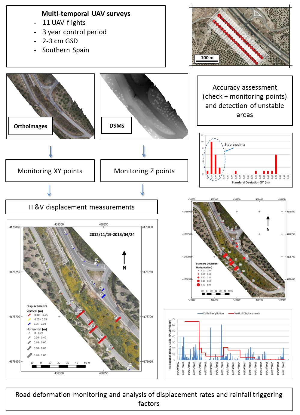
This paper presents a methodology for measuring road surface deformation due to terrain instability processes. The methodology is based on ultra-high resolution images acquired from unmanned aerial vehicles (UAVs). Flights are georeferenced by means of Structure from Motion (SfM) techniques. Dense point clouds, obtained using the multiple-view stereo (MVS) approach, are used to generate digital surface models (DSM) and high resolution orthophotographs (0.02 m GSD). The methodology has been applied to an unstable area located in La Guardia (Jaen, Southern Spain), where an active landslide was identified. This landslide affected some roads and accesses to a highway at the landslide foot. The detailed road deformation was monitored between 2012 and 2015 by means of eleven UAV flights of ultrahigh resolution covering an area of about 260 m × 90 m. The accuracy of the analysis has been established in 0.02 ± 0.01 m in XY and 0.04 ± 0.02 m in Z. Large deformations in the order of two meters were registered in the total period analyzed that resulted in maximum average rates of 0.62 m/month in the unstable area. Some boundary conditions were considered because of the low required flying height (<50 m above ground level) in order to achieve a suitable image GSD, the fast landslide dynamic, continuous maintenance works on the affected roads and dramatic seasonal vegetation changes throughout the monitoring period. Finally, we have analyzed the relation of displacements to rainfalls in the area, finding a significant correlation between the two variables, as well as two different reactivation episodes.

1. Introduction

Landslide analyses involve different types of approaches related to both engineering practice and scientific research [1], frequently allowing one to evaluate and, if possible, mitigate the risks associated with them. The workflow starts with data capture in order to identify, map and monitor landslides and their properties. In a subsequent step, stability and/or risk analyses can be carried out.

Data capture is currently done by means of several instruments and techniques that according to [2] can be classified in: satellite and remote sensing techniques, from optical spectrum to DInSAR approaches [3,4,5]; aerial photogrammetric and LiDAR techniques [6,7]; geodetic and surveying techniques [8,9]; and geotechnical and geophysical techniques [10]. The first two groups can be considered as remote sensing techniques and the last two groups as in situ techniques. From data capture, different analyses can be addressed, both for individual landslides and for regional studies. In the first case, stability analysis using conventional deterministic methods [11] and predictive methods using grey-scale or machine/deep learning methods [12] can be applied. In regional studies, susceptibility and hazard analysis can be made employing also different approaches that according to [13] can be clustered into six main groups: classical statistics (e.g., logistic regression, discriminant analysis, linear regression); index-based (e.g., weight-of evidence, heuristic analysis); machine learning (e.g., fuzzy logic systems, support vector machines, forest trees); neural networks (deep learning); multi criteria decision analysis; and other statistics.

Remote sensing combined with geographic information system (GIS) techniques allows the study of areas of different size and scale with adequate resolution and accuracy [14]. Specifically, photogrammetric techniques have been extensively used in the last decades to study landslide evolution [6,7,15,16,17,18,19,20]. In these studies, after image block orientation based on conventional aerial triangulation techniques and bundle adjustment [21], Digital Terrain or Surface Models (DTM/DSMs) are calculated using automatic matching techniques. From these models, some approaches such as differential DSM/DTMs or volumetric calculations are addressed in practically all these studies, and 3D displacement vectors are also calculated in some of them [6,15,20].

Furthermore, recent years have seen an increasing use of unmanned aerial vehicles (UAVs) of different types and dimensions for many environmental applications in which usually very high to ultrahigh resolution and precision are required. These applications have been stimulated by the improvement on the performance of these systems and also the use of new computer vision algorithms. Among the latter, those based on dense matching can be highlighted, Structure from Motion (SfM) and Multiple View Stereo (MVS) approaches [22,23,24,25,26,27]. UAVs have been applied to landslide inventory and susceptibility mapping by means of photo interpretation [28,29], risk evaluation [30,31,32] and monitoring [33,34].

Most approaches are based on the elaboration of DSM/DTMs and orthophotographs, from flights oriented by aerial triangulation and SfM/MVS methods [29,33,34,35,36,37,38,39,40,41,42,43,44,45,46,47,48,49,50,51,52,53,54,55,56,57]. In these studies the orientation of flights is based on ground control points (GCPs) measured with GNSS or transferred from previous photogrammetric flights [41,42] or LiDAR models [36]. Some authors have also undertaken experiments for direct orientation without GCPs [44,52,53], although according to other studies, at present, those methods with field surveyed GCPs produce more accurate results [58,59,60]. Both DTMs or DSMs are used for the geomorphic characterization of landslides and their features [38,39,41,42,45,52,53,54,56] or more frequently to obtain differential models for recognizing changes of the terrain surface [34,36,38,39,40,41,42,46,47,50,52,53,54,55,56,57], volumetric calculations [34,36,41,42,50,54,55,56,57] and profiles [34,36,48,50,54,55,57].

Meanwhile, orthophotographs also allow the recognition of features and landslide description [34,36,38,41,42,48,54,56,57] and in a particular way the accurate calculation of the horizontal displacements between significant points [34,35,38,39,41,42,46,47,48,49,50,54,55]. In most of these cases the significant points are selected and extracted manually, although some experiments using automatic measurements of displacements have been proposed based on shaded relief, tree displacements or other geomorphic attributes [34,42,52,53]. In any case the analyses of DTM/DSMs and/or orthophotographs are the basis of evolutionary studies of landslides, sometimes combined with other techniques such as GNSS, tachymetric surveys, terrestrial/aerial photogrammetry and terrestrial/aerial LiDAR. Finally, other products such as videos have been obtained [56,57] in order to show instantaneous or rapid movements and estimate the velocities and volumes involved.

To ensure the quality of the analyses, especially the multitemporal ones, the assessment of positional accuracy is of prime importance. This can be done during the accuracy analysis in relation with the photogrammetric orientation processes [36,38,41,42,43,46,50,58,59], the derived DSM/DTMs and orthophotographs [36,38,41,42,46,47,54,59] or the 3D-point clouds [34,51,52,53].

In this study a method for the analysis of road surface deformation has been developed, from images captured by means of eleven ultrahigh resolution (UHR) UAV flights. It is based on photogrammetric orientation by means of SfM-MVS techniques with the support of GCPs measured with DGNSS and a later generation of DSMs and orthophotographs. A set of monitoring points were extracted manually from the orthophotographs and the DSMs, since automatic extraction was not feasible because of the intense deformation of the road surface due to successive episodes of destruction and re-asphalting. The calculation of basic statistics of coordinates and displacements of monitoring points between different epochs has allowed the identification of an unstable zone as well as the determination of its kinematics and the relationships with the rainfalls as triggering factor.

2. Study Area

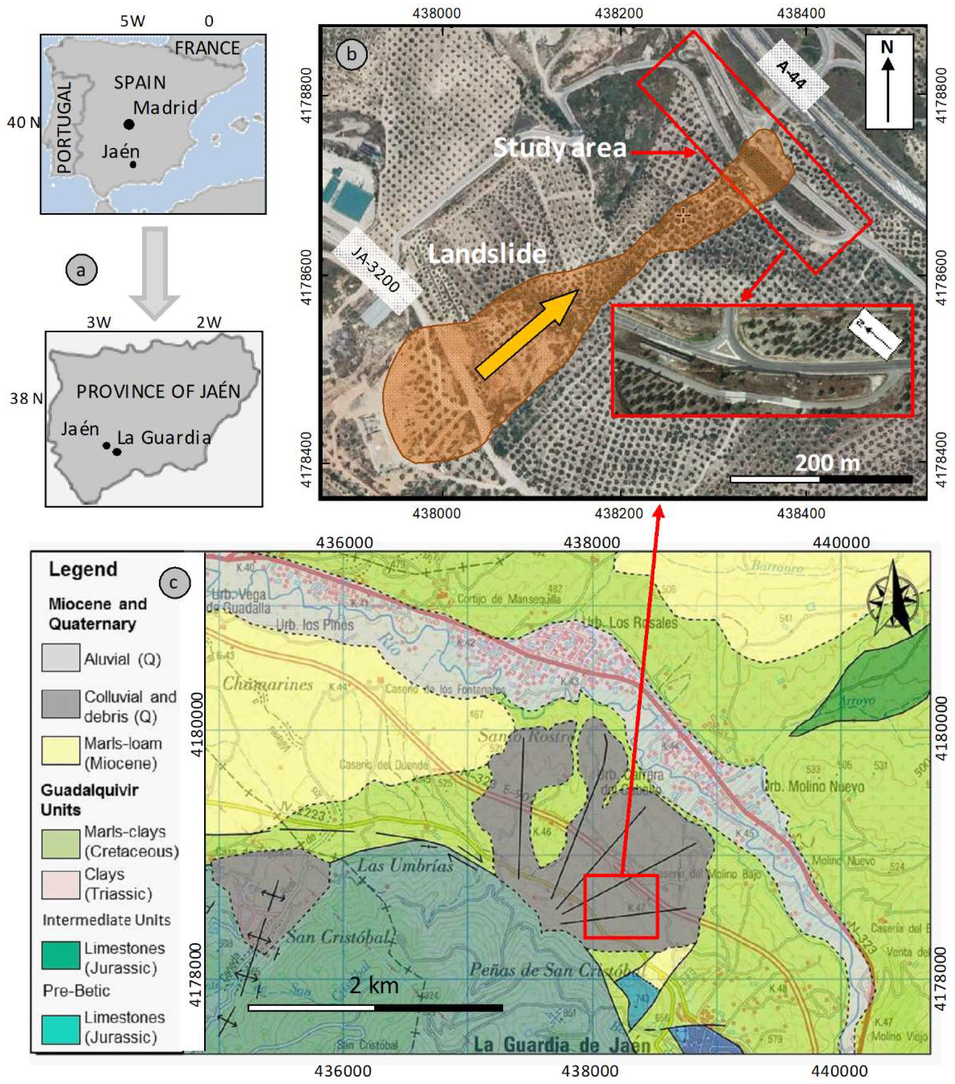
The study area is located near the village of La Guardia de Jaén, Southern Spain (Figure 1a), in a landslide foot that affects an olive grove and several roads, such as the access to the village from the A-44 highway and other service roads (Figure 1b,c). This area is near the University of Jaén and it is used as a natural lab, with many evidences of landslides in the hillslopes surrounding it [61,62], most of them corresponding to earth flows and also to slides [41,63,64].

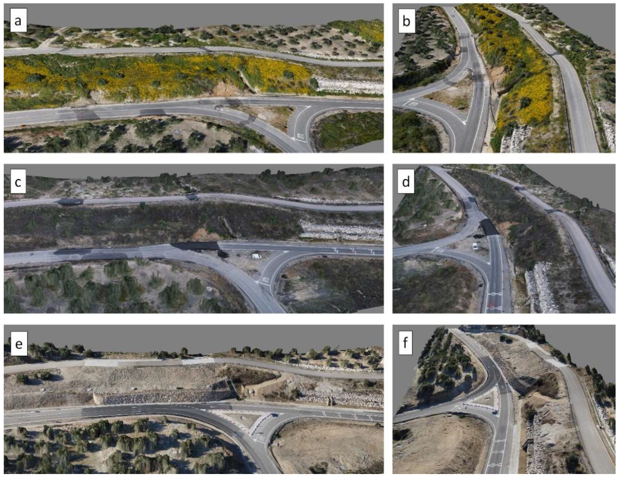
Specifically, the landslide corresponds to an earth flow with an approximate extension of 500 m in length, 50–150 m width and a height difference of 80 m, as it has been described in previous studies [42]. The movement remained active for a period close to two years until finally it was stabilized and the roads repaired (Figure 2).

In the study area the geological Guadalquivir Units outcrop [66]. These units consist in a set of materials with a complex structure and diverse lithology, in which the following formations predominate: Triassic evaporites and shales, Cretaceous-Paleogene marls and clays, and Miocene loamy-clay sediments belonging to the Guadalquivir basin. In this area the Guadalquivir Units are represented by marls and clays overthrusted by thick stratigraphic successions of Jurassic limestones from Intermediante Betic Units, which form a prominent relief (Figure 1c) [65,66,67,68]. The contact is dotted with small alluvial fans, thick piedmont deposits and travertines, the last associated with springs at the foot of the Jurassic limestones.

3. Materials and Methods

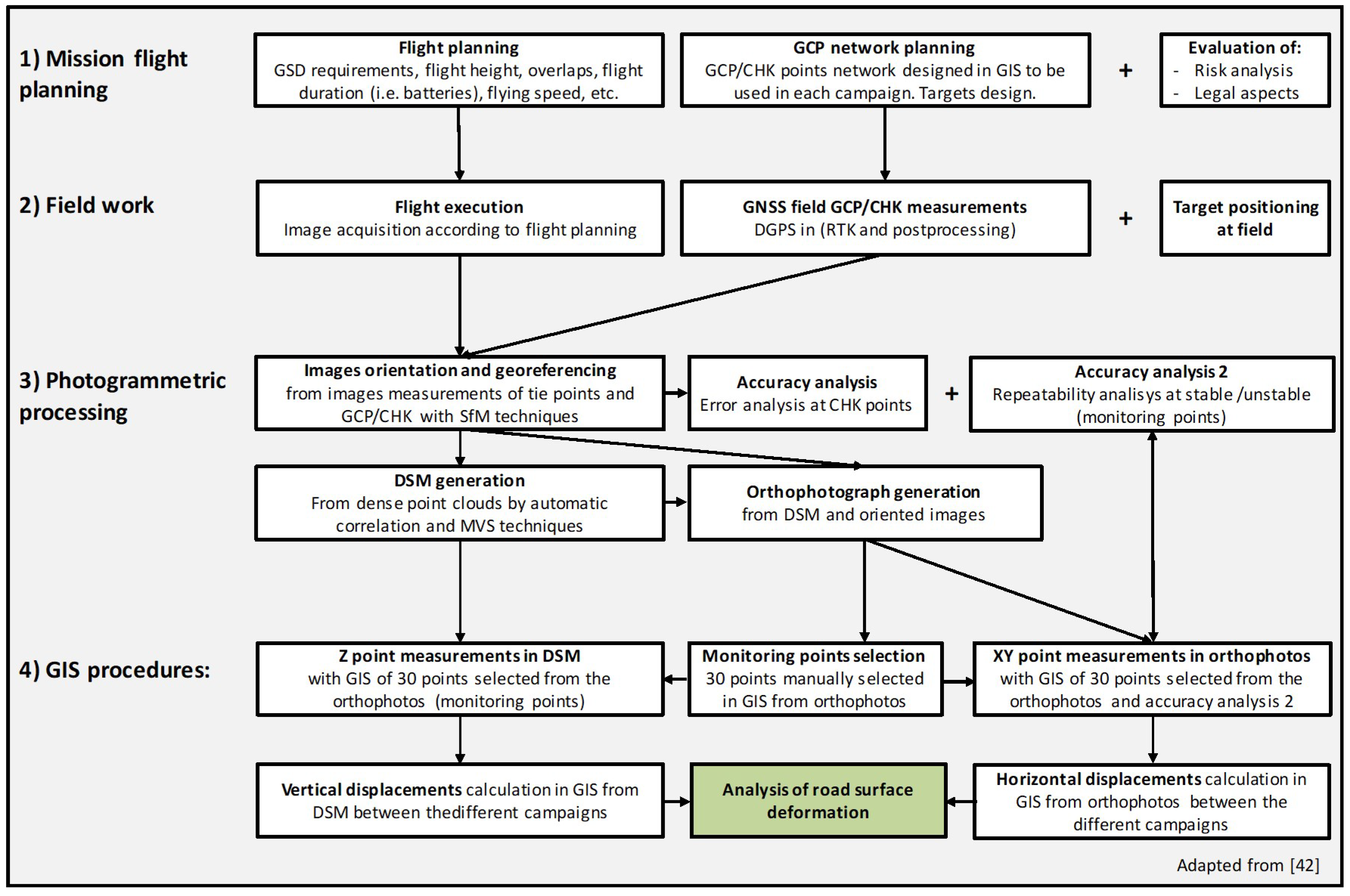
The methodology was based on aerial photogrammetry techniques used in previous landslide monitoring studies by the authors [7,16,41,42,49,69]. Such methodologies were adapted to the case study analyzed in this paper since some boundary conditions had to be taken into consideration. Some of these constraints were the use of UAV, the low flying height (<50 m above ground level), the fast landslide dynamic, maintenance works on the affected roads and dramatic seasonal vegetation changes throughout the monitoring period. Due to the large photo-scale, great differences between images at different dates were found, so identification of same areas at that GSD was a challenging task. The methodology can be summarized in the following steps (Figure 3):

• Flight planning: selection of UAV equipment and mission planning.
• Field work: GNSS field survey and execution of flights.
• Photogrammetric processing 1: georeferencing and flight orientation with SfM techniques.
• Photogrammetric processing 2: DSM and orthophotograph generation.
• GIS procedures and deformation analysis: measurement of displacements at identifiable points between campaigns.

3.1. Data Capture: UAV Flights and Field Work

The flights were executed with an eight-rotor AscTec Falcon 8 [70] coupled with GNSS/INS and equipped with an NEX 5N mirrorless interchangeable lens camera (MILC, APS-C format, 16 Mpx, pixel size 4.9 μm, Sony, Tokyo, Japan). The maximum takeoff weight (MTOW) of the Falcon 8 is 2.3 kg and its speed is in the range of 4.5 to 15 m/s depending on the flight mode (manual, height or GPS mode). Due to the low flying height, the selected speed was 5 m/s to avoid blurred images from forward motion errors. For this study, eleven ultra-high resolution and accuracy UAV flights were carried out between November 2012 and November 2015. The flight characteristics are shown in

Table 1. Properties of photogrammetric flights.

No.	Date	No. Images	GSD (m)	Flying Height (m)
1	19 November 2012	25	0.030	100 *
2	24 April 2013	44	0.011	41
3	03 May 2013	50	0.011	39
4	20 May 2013	48	0.011	40
5	04 July 2013	47	0.014	50
6	17 January 2014	46	0.012	43
7	05 March 2014	43	0.013	45
8	16 July 2014	24	0.034	105 *
9	23 December 2014	44	0.012	44
10	27 March 2015	44	0.013	46
11	19 November 2015	47	0.013	45

* These flights are part of a wider surveyed area [42].

and their location and extension in Figure 4.

In all cases, the flights followed a conventional photogrammetric pattern with vertical photographs and image overlaps of the order of 70–80% to guarantee a proper vertical accuracy and enough redundancy [21]. However, there were two flight groups with different image block geometry. On the one hand, most of the aerial surveys were planned at flying heights lower than 50 m above mean ground level. Two strips were carried out with 22–25 images per strip. Such flying heights guaranteed a GSD of <2 cm. These flights were planned to survey the sections of the roads affected by the landslide and they covered an area of some 260 m × 85 m (Figure 4).

On the other hand, two flights were flown between 100 m and 120 m above the mean terrain height, which guaranteed a ground sample distance (GSD) always lower than 0.05 m. Flying heights were kept under 400 feet above mean ground level (approximately 120 m), bearing in mind the maximum height limit allowed by the Spanish regulations for the use of RPAS. These flights were planned at higher altitude as part of a wider monitoring analysis of the whole slope affected by the landslide [42]. Although the GSD on the affected area of that paper was different, the inclusion of these two flights in the present paper was considered pertinent at the beginning of the analysis (February 2012) and at the middle of the control period (July 2014).

3.2. Georeferencing and Flight Orientation

For the orientation of the UAV image blocks, a GCP network was planned for each flight. These GCPs were defined as targets. These targets were reusable circular white/black targets printed on PVC foam board, disposable painted targets on the ground and some well-defined natural points (Figure 5). GCPs were surveyed with differential GNSS methods (DGNSS) in the centimeter accuracy range with LeicaSystem 1200 and Leica Viva systems (Leica Geosystems, Heerbrugg, Switzerland). A set of these points was not used in the orientation process, but they were reserved as check points (CHKs) for validating the accuracy of this process (

Table 2. Orientation errors.

Date	GSD	GCP/CHK Number	Tie Point Number	RMS Pixel	CHK RMS (m)
					RMS XY (m)	RMS Z (m)
19 November 2012	30	11/5	151,635	0.37	0.018	0.012
24 April 2013	11	9/3	356,966	0.41	0.024	0.015
03 May 2013	11	11/4	367,430	0.39	0.014	0.014
20 May 2013	11	17/4	59,384	0.82	0.013	0.023
04 July 2013	14	12/6	9479	0.83	0.017	0.010
17 January 2014	12	7/3	423,343	0.43	0.026	0.005
05 March 2014	12.5	7/3	426,766	0.54	0.019	0.004
16 July 2014	33.8	7/4	247,888	0.86	0.030	0.032
23 December 2014	12.4	14/6	101,414	0.57	0.016	0.010
27 March 2015	12.7	13/9	62,348	0.81	0.011	0.010
19 November 2015	12.6	10/4	60,277	0.71	0.022	0.027
Mean				0.66	0.020	0.016
STD				0.25	0.007	0.009

). Blocks were oriented in the ETRS89/UTM 30N coordinate reference system (CRS).

Unlike previous landslide monitoring studies by the authors [7,42], it was not possible to transfer a sufficient numbers of points between different campaigns (second-order GCPs). As shown by these previous studies, taking one of the surveys as common reference reduces the field work as a cost-saving technique. Moreover, the use of points transferred between different epochs helps to improve the geo-referencing of all sets of images in a common reference system, facilitating the comparison between the models and orthoimages generated from them. This is possible if there are stable natural points, unambiguously identifiable and well distributed throughout the area. But since the flights used in this study were limited to the affected area near the roads, it was difficult to identify stable natural points in large sections of the surveyed area due to the intense landslide dynamic as well as the continuous maintenance works. These circumstances, which were modifying the terrain dramatically during the monitoring period, advised against the use of any permanent benchmark. Consequently, GCPs were measured in the field by means of GNSS to register each flight, otherwise no stable ground control points in the central part of the area could have been transferred from a reference flight.

The images were processed and aligned by means of dense matching and Structure from Motion (SfM) techniques, which implied the automatic measurement of some tens of thousands of common tie points. After the measurement of the GCPs and CHKs, the final photogrammetric orientations were computed using a global bundle block adjustment [21,22,23]. All processes were implemented with Agisoft PhotoScan software [24]. The errors in the check points, expressed as RMS, refer to the residuals calculated in these points after the bundle adjustment. The final accuracies of all adjustments are shown in Table 2. Errors at the check points do not exceed 0.035 m in both XY and Z in any case.

An additional error check was carried out in order to review the orientation process of all the flights, bearing in mind that all of them had been registered with different GCPs. Thus a set of 30 natural points identifiable in as many flights as possible were selected and located in both stable and unstable areas. These points (monitoring points) were measured in the orthophotographs and the DSMs. Due to terrain changes not all points could be measured in all epochs, especially those points located in the affected areas where the destruction and reparation of roads took place. The errors (uncertainties) were estimated by means of the calculation of basic statistics of stable points (

Table 3. Standard deviations of the monitoring points coordinates along the different epochs.

Points	Number of Measurements	SDXY (m)	SDZ (m)
1	11	0.017	0.039
2	11	0.018	0.064
3	11	0.009	0.030
4	11	0.018	0.053
5	11	0.017	0.041
6	11	0.019	0.070
7	11	0.017	0.021
8	8	0.017	0.036
9	8	0.027	0.017
10	8	0.037	0.061
11	10	0.030	0.050
12	8	0.012	0.015
13	8	0.012	0.024
14	11	0.030	0.045
15	11	0.026	0.068
16	11	0.623	0.062
17	10	0.616	0.114
18	11	0.026	0.056
19	11	0.022	0.030
20	10	0.611	0.070
21	10	0.554	0.098
22	11	0.609	0.090
23	11	0.621	0.070
24	10	0.628	0.070
25	10	0.071	0.019
26	5	0.025	0.019
27	10	0.482	0.082
28	10	0.020	0.051
29	7	0.231	0.122
30	6	0.371	0.192
Total	Mean (m)	0.194	0.059
	STD (m)	0.257	0.038
Stable area 1	Mean (m)	0.021	0.042
	STD (m)	0.007	0.018
Unstable area 2	Mean (m)	0.492	0.090
	STD (m)	0.190	0.044

¹ Points at stable area: SD_XY < 0.04 m; ² Points at unstable area: SD_XY > 0.04 m.

, these results will be presented in Section 4.1).

3.3. DSM and Orthophotograph Generation

The Digital Surface Models (DSMs) of all flights were generated from a densification of the initial sparse point cloud (using the dense point cloud tool of PhotoScan) after the block orientation. Then orthoimages for each campaign were also generated. Finally, both products were exported as raster files (TIFF) to be incorporated into GIS analysis.

In conventional photogrammetry the resolution of a digital model is several times that of the GSD of the original images. But in this paper, given dense matching techniques used by the current SfM and MVS photogrammetric software and taking into account the dimensions of the area and the characteristics of the flights, the selected pixel size of the DSMs was twice that of the orthoimages (0.04 m). The resolution of the orthophotographs was 0.02 m. This value was selected given the GSD values of the original images (Table 1), the errors given after the analysis of check points (Table 2) and analysis of the monitoring points in stable areas (Table 3, in the next section), which are of the same order of magnitude than the resolution. Therefore measurements made on the orthoimages can be considered as reliable.

Unlike other previous studies [7,41,42], in this paper the main objective was to monitor the road deformation caused by the landslide. For this purpose, we have used points extracted from DSMs and orthophotographs in the road areas, from which horizontal and vertical displacements have been computed. We have dismissed the use of differential DTM/DSMs by different reasons. First in the margins of roads there is a high density of vegetation with grass, scrubs and bushes that had grown intensely in the study period. Under this circumstance reliable DTMs would have not been obtained from DSMs since the vegetation could not be removed using tools of point clouds classification and filtering. Moreover, the stereo-model edition using photogrammetric workstations would have not ensured good results and would have been time-consuming. Therefore the analysis was focused in road areas, where DTMs and DSMs coincide. Moreover, since the maintenance works had changed the road surface at the critical areas (the roads have been asphalted several times throughout the control period), we cannot compare directly DSMs between different epochs, but natural points identifiable throughout the study period.

3.4. Measurement of Displacements

The comparison between the different epochs for monitoring road deformation has been based on the calculation of displacements of the set of 30 monitoring points extracted manually from DSM and orthophotographs (the monitoring points mentioned earlier in Section 3.2). The monitoring points were selected manually and located carefully on the roads surfaces at well-identifiable features such as road reflective markers and corners on road surface markings. Automatic extraction of points has not been feasible because of the intense deformation of the road surface due to successive episodes of destruction and re-asphalting.

Then the coordinates of those points were measured in the DSM (Z) and orthophotographs (XY), and the vertical and horizontal displacements were calculated, subtracting their coordinates in different epochs. These operations were performed with QGIS open source software [71].

4. Results

In this section the results of the analysis carried out from the coordinates of the monitoring points is presented: (1) we have determined basic statistics of these points in order to identify stable and unstable zones, and to estimate the uncertainties of the measurements; (2) we have computed point displacements; and (3) the corresponding rates, in order to monitor the road deformation.

4.1. Basic Statistics of Monitoring Points

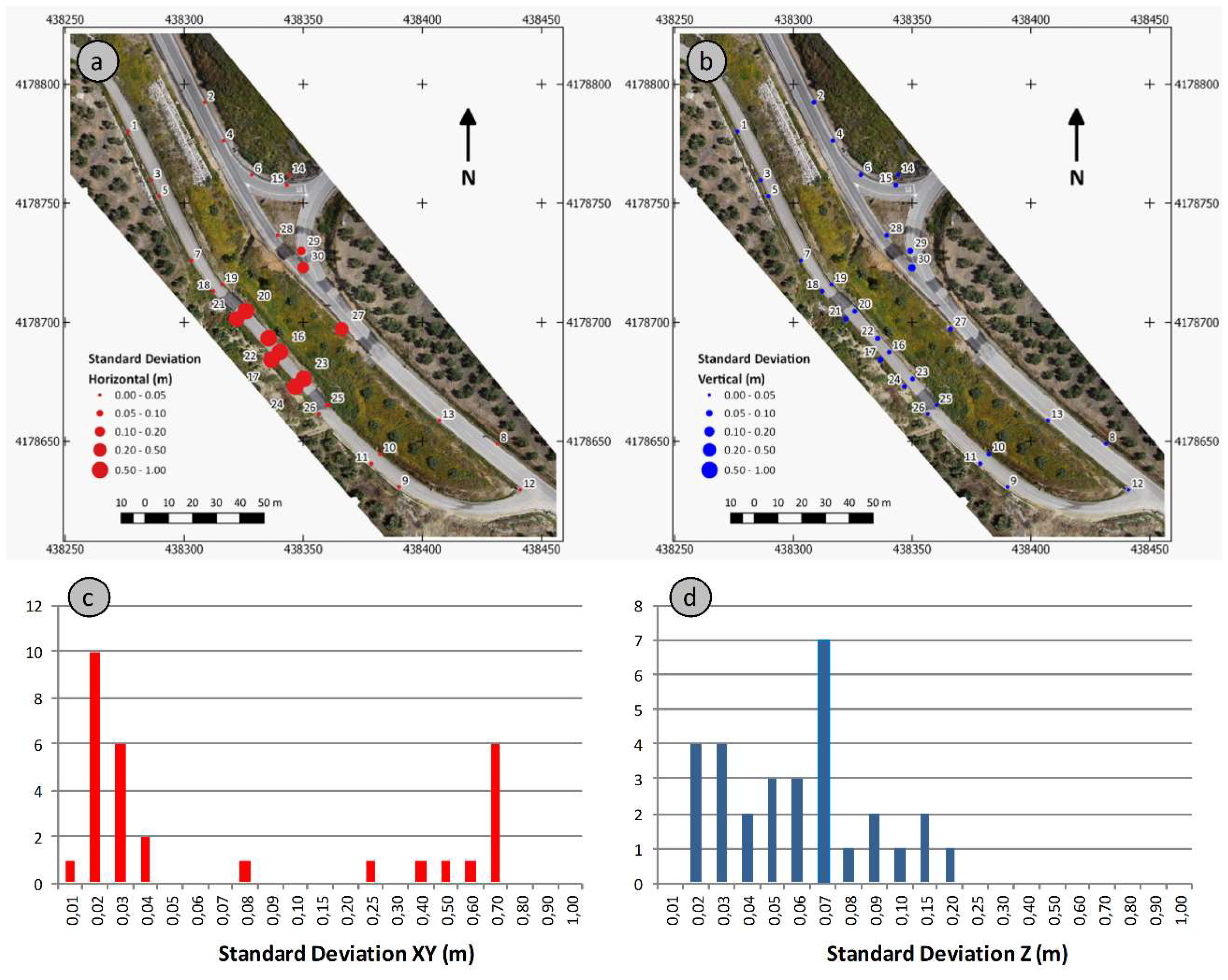
The standard deviation (SD) of the monitoring points coordinates is shown in Table 3 and the maps of the Figure 6. Every point appears in at least five epochs and many of them appear in 10–11 epochs, so the deformation can be measured adequately. The analysis of the SD distribution of monitoring points has allowed the accurate identification and delimitation of the unstable and unstable zones, besides the estimation of errors and uncertainties before explained.

From Table 3, first we can observe that in general SD showed higher values and variability in the horizontal (XY) than in the vertical component (Z). Moreover, there are two types of points, based on SD XY values (Figure 6a,b): those with lower values (around 0.02 m) and those with higher values (around 0.50 m). These types can be distinguished clearly in the map of Figure 6a and in the histogram of Figure 6b, corresponding to a stable area (at the margins) and unstable area (at the center), respectively. Points located in the stable area show a uniform SD in XY, always lower than 0.04 m. A certain graduation of SD values in the unstable area could be observed and thus the maximum values of SD were observed in the central area (points 16, 17, 22, 23, 24), decreasing to the north-western margin (points 20 and 21, and especially 29 and 30), to the north-eastern foot (point 27) and to the south-eastern margin (point 25). Meanwhile, in the stable area the points with SD values slightly higher are those near the limit of the unstable area (points 10, 11, 18, 26 and 28).

Regarding SD Z (Figure 6c,d), there are certain differences between points belonging to stable and unstable point zones (mean values of 0.04 and 0.09) but much smaller than in the horizontal component. Nevertheless the higher values were reached again in the points of the central area (points 16, 17, 20, 21, 22, 23, 24 and 27), but the maximum values correspond to points at the south-eastern margin (29 and 30). Again, slightly higher values of the stable area were reached in points near the margin of the stable area (points 6 and 10).

4.2. Displacements of Monitoring Points

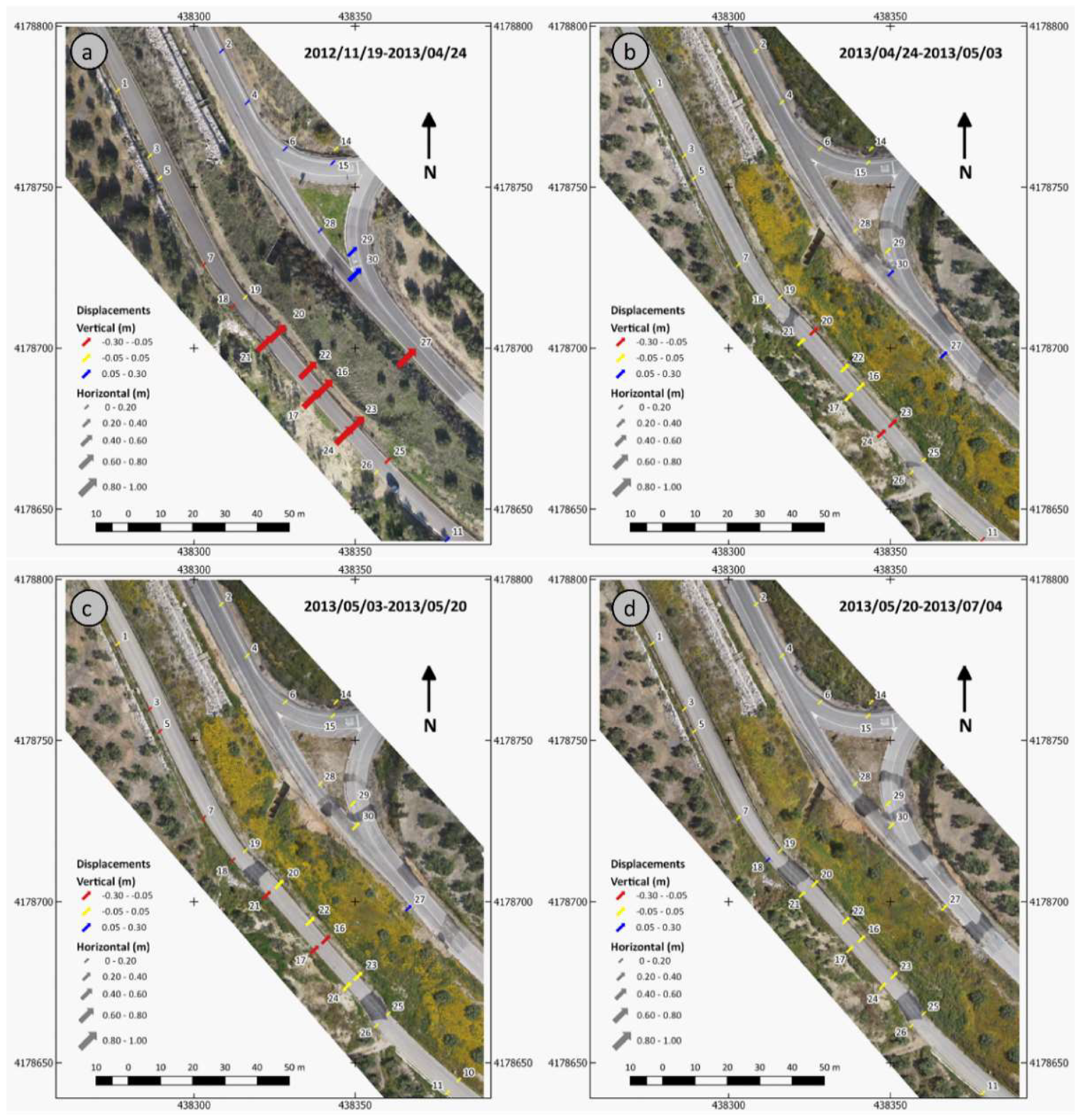
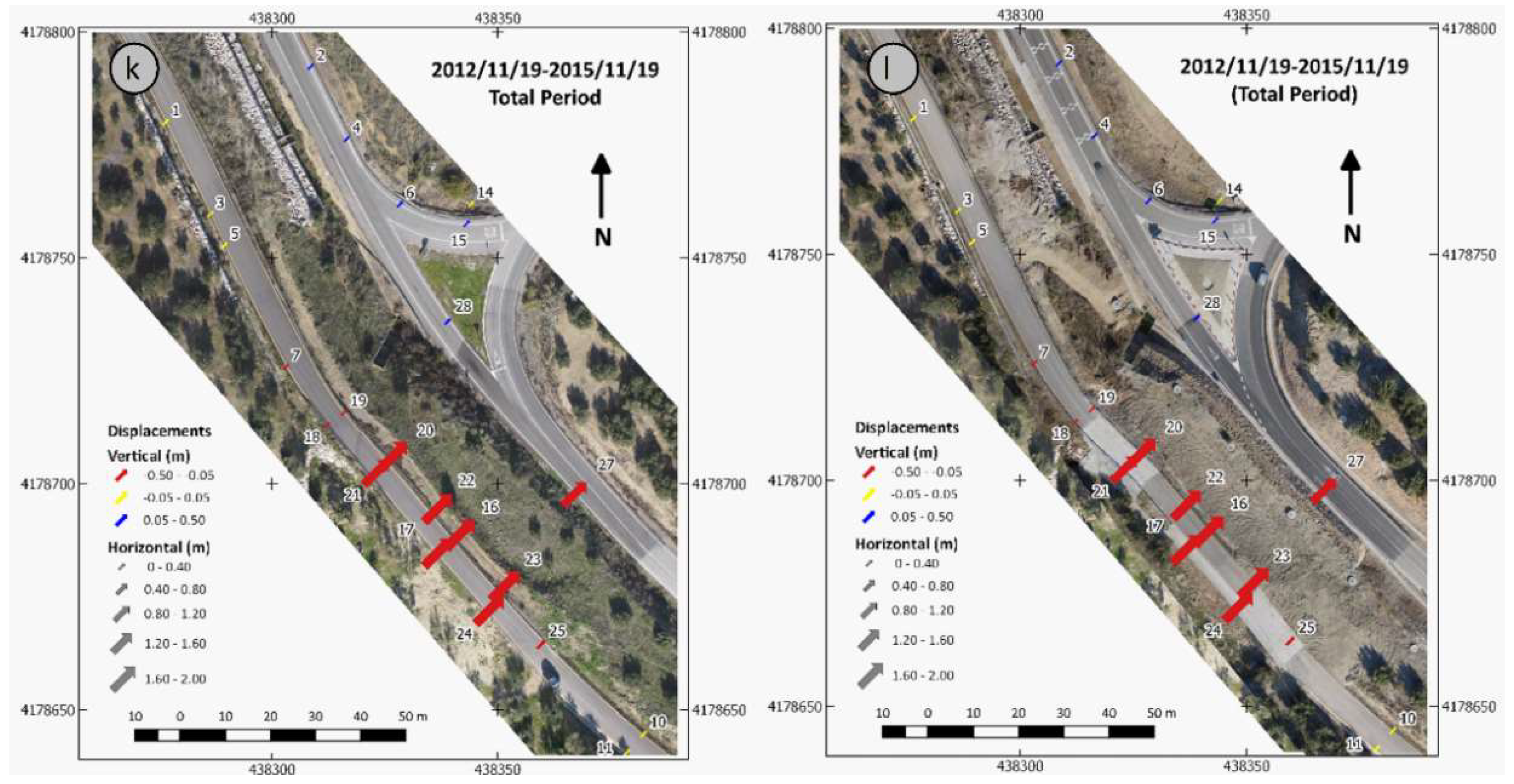
The displacements of the extracted points on roads are shown in

Table 4. Horizontal (XY) displacements (in m) of the monitoring points in the different periods.

Periods	1	2	3	4	5	6	7	8	9	10	Total
Total area
Mean	0.306	0.092	0.091	0.058	0.048	0.104	0.089	0.039	0.018	0.017	0.675
SD	0.355	0.098	0.103	0.059	0.020	0.114	0.080	0.018	0.008	0.017	0.896
Min	0.005	0.006	0.007	0.003	0.015	0.005	0.001	0.011	0.006	0.000	0.006
Max	0.838	0.253	0.277	0.172	0.093	0.289	0.231	0.085	0.033	0.058	2.005
Stable area
Mean	0.027	0.018	0.025	0.019	0.037	0.023	0.028	0.032	0.019	0.019	0.027
SD	0.014	0.008	0.012	0.009	0.014	0.011	0.024	0.011	0.009	0.011	0.020
Min	0.005	0.006	0.007	0.003	0.015	0.005	0.001	0.011	0.008	0.000	0.006
Max	0.053	0.035	0.046	0.041	0.063	0.041	0.070	0.045	0.033	0.031	0.078
Unstable area
Mean	0.660	0.186	0.205	0.123	0.065	0.218	0.170	0.048	0.017	0.015	1.684
SD	0.235	0.076	0.091	0.049	0.017	0.092	0.050	0.023	0.009	0.024	0.574
Min	0.139	0.032	0.016	0.016	0.040	0.019	0.072	0.017	0.006	0.000	0.206
Max	0.838	0.253	0.277	0.172	0.093	0.289	0.231	0.085	0.033	0.058	2.005

Periods: 1 (19 November 2012–24 April 2013); 2 (24 April 2013–3 May 2013); 3 (3 May 2013–20 May 2013); 4 (20 May 2013–4 July 2013); 5 (4 July 2013–17 January 2014); 6 (17 January 2014–5 March 2014); 7 (March 2014–16 July 2014); 8 (16 July 2014–23 December 2014); 9 (23 December 2014–27 March 2015); 10 (27 March 2015–19 November 2015).

and

Table 5. Vertical (Z) displacements (in m) of the monitoring points in the different periods.

Periods	1	2	3	4	5	6	7	8	9	10	Total
Total area
Mean	−0.027	−0.020	−0.013	−0.002	−0.005	0.004	−0.019	0.001	0.011	−0.018	−0.084
SD	0.132	0.037	0.046	0.042	0.051	0.027	0.102	0.091	0.041	0.021	0.156
Min	−0.269	−0.089	−0.098	−0.074	−0.115	−0.039	−0.267	−0.227	−0.153	−0.055	−0.315
Max	0.253	0.082	0.100	0.139	0.057	0.075	0.226	0.232	0.057	0.024	0.145
Stable area
Mean	0.021	−0.021	−0.011	−0.004	0.018	−0.005	−0.021	0.006	0.012	−0.019	0.011
SD	0.087	0.027	0.041	0.049	0.043	0.022	0.065	0.053	0.016	0.023	0.105
Min	−0.202	−0.089	−0.098	−0.074	−0.115	−0.039	−0.118	−0.070	−0.021	−0.055	−0.244
Max	0.124	0.014	0.061	0.139	0.057	0.041	0.083	0.091	0.037	0.024	0.145
Unstable area
Mean	−0.088	−0.019	−0.016	0.001	−0.041	0.016	−0.015	−0.005	0.010	−0.014	−0.232
SD	0.156	0.049	0.056	0.028	0.042	0.029	0.142	0.129	0.064	0.009	0.093
Min	−0.269	−0.072	−0.078	−0.026	−0.115	−0.017	−0.267	−0.227	−0.153	−0.024	−0.315
Max	0.253	0.082	0.100	0.052	0.019	0.075	0.226	0.232	0.057	−0.007	−0.068

Periods: 1 (19 November 2012–24 April 2013); 2 (24 April 2013–3 May 2013); 3 (3 May 2013–20 May 2013); 4 (20 May 2013–4 July 2013); 5 (4 July 2013–17 January 2014); 6 (17 January 2014–5 March 2014); 7 (March 2014–16 July 2014); 8 (16 July 2014–23 December 2014); 9 (23 December 2014–27 March 2015); 10 (27 March 2015–19 November 2015).

and the maps of Figure 7. The total displacements vary from values lower than 0.01 m to higher than 2 m in the horizontal component (Table 4). Thus, the stable area shows average displacements of about 0.03 m with a low dispersion (SD of 0.02 m), while the unstable area, at the center of the map, shows average displacements of about 1.68 m and higher dispersion (SD of 0.57 m). Here it can be also observed a graduation. The maximum values of total horizontal displacements (near to 2 m) were observed in the center of the unstable area (points 16, 17, 22, 23, 24). Then displacements decrease to the northwestern margin (points 20 and 21, with displacements of about 1.8 m), the northeastern foot (point 27 with displacement of 1.5 m) and the southeastern margin (point 25, where the displacement is of 0.21 m, clearly lower). Meanwhile, in the stable area the points with slightly higher displacements (about 0.07 m) are those near the limit of the unstable area (points 10 and 11).

Regarding the vertical component, it presents significantly lower values (Table 5), from −0.32 to 0.15 m, with average values of 0.01 m in the stable area and -0.23 m in the unstable area (a small descent of the ground surface), also with low dispersion (about 0.10 m in both areas). Thus, the greater descents observed in the monitoring points were reached again in the central area (points 16, 17, 20, 21, 22, 23 and 24 with displacements around 0.20–0.30 m), but also in some points at the margins (7, 18, 19, 25 and 28). Besides there are some points where a certain ascent of about 0.10 m was observed (2, 4, 6, 15 and 28), all of them located in the lower sector of the studied area (landslide foot and the access road to the highway).

By periods, the average of horizontal displacements shows little variability in the stable area, oscillating from values near to 0.02 m in several periods to near 0.04 m in the 4 July 2013–17 January 2014 period. However, in the unstable area the variability was much higher and thus it presented a high average value of 0.66 m in the first period (19 November 2012–24 April 2013); then two periods with values near 0.20 m (24 April 2013–3 May 2013 and 3 May 2013–20 May 2013); later, two periods in which the average displacements descend below 0.10 m (20 May 2013–4 July 2013 and 4 July 2013–17 January 2014), followed by two new periods in which the average displacements again reached values near 0.20 m (17 January 2014–5 March 2014 and 5 March 2014–16 July 2014); and finally, values lower than 0.05 m and even 0.02 m were observed in the last three periods (16 July 2014–23 December 2014, 13 December 2014–27 March 2015 and 27 March 2015–19 November 2015).

Meanwhile, the average vertical displacements in the stable area also presented values that barely reached 0.02 m in absolute terms for every period analyzed. In the unstable area negative values predominated (descent of terrain), but only during the first period (19 November 2012–24 April 2013) significant values near to 0.10 m were reached.

4.3. Displacements Rates of Monitoring Points

The displacements rates of the extracted points at roads are shown in

Table 6. Horizontal displacement rates (in m/month) of monitoring points in the different periods.

Periods	1	2	3	4	5	6	7	8	9	10	Total
Total area
Mean	0.059	0.305	0.161	0.040	0.007	0.062	0.020	0.007	0.006	0.002	0.019
SD	0.069	0.328	0.182	0.040	0.003	0.071	0.018	0.004	0.003	0.002	0.025
Min	0.001	0.020	0.012	0.002	0.002	0.000	0.000	0.002	0.002	0.000	0.000
Max	0.162	0.844	0.489	0.117	0.015	0.181	0.053	0.016	0.011	0.008	0.056
Stable area
Mean	0.005	0.059	0.045	0.013	0.006	0.013	0.006	0.006	0.006	0.002	0.001
SD	0.003	0.026	0.020	0.006	0.002	0.008	0.005	0.002	0.003	0.001	0.001
Min	0.001	0.020	0.012	0.002	0.002	0.000	0.000	0.002	0.002	0.000	0.000
Max	0.010	0.117	0.081	0.028	0.010	0.026	0.016	0.009	0.010	0.004	0.002
Unstable area
Mean	0.128	0.619	0.362	0.084	0.010	0.136	0.039	0.009	0.005	0.002	0.047
SD	0.045	0.253	0.160	0.033	0.003	0.058	0.011	0.004	0.003	0.003	0.016
Min	0.027	0.108	0.028	0.011	0.006	0.012	0.017	0.003	0.002	0.000	0.006
Max	0.162	0.844	0.489	0.117	0.015	0.181	0.053	0.016	0.011	0.008	0.056

Periods: 1 (19 November 2012–24 April 2013); 2 (24 April 2013–3 May 2013); 3 (3 May 2013–20 May 2013); 4 (20 May 2013–4 July 2013); 5 (4 July 2013–17 January 2014); 6 (17 January 2014–5 March 2014); 7 (March 2014–16 July 2014); 8 (16 July 2014–23 December 2014); 9 (23 December 2014–27 March 2015); 10 (27 March 2015–19 November 2015).

and

Table 7. Vertical displacement rates (in m/month) of monitoring points in the different periods.

Periods	1	2	3	4	5	6	7	8	9	10	Total
Total area
Mean	−0.005	−0.067	−0.023	−0.002	−0.001	0.002	−0.004	0.000	0.004	−0.002	−0.002
SD	0.025	0.125	0.082	0.028	0.008	0.016	0.023	0.017	0.013	0.003	0.004
Min	−0.052	−0.296	−0.172	−0.050	−0.018	−0.024	−0.061	−0.043	−0.049	−0.007	−0.009
Max	0.049	0.275	0.177	0.095	0.009	0.047	0.052	0.044	0.018	0.003	0.004
Stable area
Mean	0.004	−0.069	−0.020	−0.003	0.003	−0.003	−0.005	0.001	0.004	−0.002	0.000
SD	0.017	0.090	0.072	0.033	0.007	0.013	0.015	0.010	0.005	0.003	0.003
Min	−0.039	−0.296	−0.172	−0.050	−0.018	−0.024	−0.027	−0.013	−0.007	−0.007	−0.007
Max	0.024	0.047	0.108	0.095	0.009	0.026	0.019	0.017	0.012	0.003	0.004
Unstable area
Mean	−0.017	−0.064	−0.028	0.001	−0.006	0.010	−0.003	−0.001	0.003	−0.002	−0.006
SD	0.030	0.164	0.099	0.019	0.007	0.018	0.033	0.025	0.020	0.001	0.003
Min	−0.052	−0.241	−0.138	−0.018	−0.018	−0.010	−0.061	−0.043	−0.049	−0.003	−0.009
Max	0.049	0.275	0.177	0.035	0.003	0.047	0.052	0.044	0.018	−0.001	−0.002

Periods: 1 (19 November 2012–24 April 2013); 2 (24 April 2013–3 May 2013); 3 (3 May 2013–20 May 2013); 4 (20 May 2013–4 July 2013); 5 (4 July 2013–17 January 2014); 6 (17 January 2014–5 March 2014); 7 (March 2014–16 July 2014); 8 (16 July 2014–23 December 2014); 9 (23 December 2014–27 March 2015); 10 (27 March 2015–19 November 2015.

. The displacement rates of the whole monitoring period (three years exactly) vary from null values to higher than 0.05 m/month in the horizontal component. The stable area showed average displacement rates practically null, while the unstable area showed average displacement rates near to 0.05 m/month with a SD of 0.16 m/month. Regarding the vertical component, it presented values practically null even in the unstable area.

More interesting and explanatory are the results by periods (Figure 8). Regarding the horizontal component, the stable area presented low values, near to 0 in most periods, except the second (24 April 2013–3 May 2013) and the third (3 May 2013–20 May 2013) in which the rates are about 0.05 m/month. The standard deviation also showed low values, especially since the fourth period (20 May 2013–4 July 2013). Meanwhile, the unstable area presented average displacement rates more variable. Thus it is started with a low rate (0.13 m/month, although the absolute displacement was higher, 0.66 m) in the first period (19 November 2012–24 April 2013). Then the rates increase strongly, reaching a value of 0.62 m/month in the second period (24 April 2013–3 May 2013) and 0.36 m/month in the third period (3 May 2013–20 May 2013). Later the displacement rate slowed to 0.08 m/month in the fourth period (20 May 2013–4 July 2013) and especially to 0.01 m/month in the fifth period (4 July 2013–17 January 2014). After this the movement reactivated and the rate again reached higher values of 0.14 m/month in the sixth period (17 January 2014–5 March 2014), but later the movement slowed again down to 0.04 m/month in the seventh period (5 March 2014–16 July 2014). Finally, the rates dropped to values under 0.01 m/month in the last three periods (16 July 2014–23 December 2014, 23 December 2014–27 March 2015 and 27 March 2015–19 November 2015). The SD of displacement rates showed only significant values in the first three periods, which allowed some points to reach maximum displacement rates of 0.16 m/month in the first period, 0.84 m/month in the second one and 0.49 m/month in the third one.

The vertical component showed average displacement rates with very low and negative values in the stable area, with some exceptions such as the second period (24 April 2013–3 May 2013) with average descent rates of -0.07 m/month and close to -0.30 m/month in some points. The unstable area also presented very low displacement rates with the exception of the second period (24 April 2013–3 May 2013) with average of -0.06 m/month and maximum descent rates of -0.24 m/month (although similar positive or ascent ratios were also reached).

5. Discussion

Firstly, some considerations about the limits of accuracy and uncertainties of the study should be addressed. Then the analysis of horizontal and vertical displacements, and especially of the displacement rates, will provide us with knowledge movement kinematics and the road deformation as well as their relationships with rainfalls as a triggering factor.

5.1. Accuracies and Uncertainties

Regarding the orientation process, the values of RMS errors at check points (measured with DGNSS in the field) were always lower than 0.035 m and in most cases lower than 0.02 m in XY and Z, and thus of the same order as the image resolution. This has been described in previous comparable studies [38,40,42,43,46,47,50,52,53] with similar properties (equipment, flight altitude and resolution).

The other test performed on the DSMs and orthophotographs also showed values compatible with this. Thus, the standard deviation (SD) of coordinate points extracted from DSMs and orthophotographs (monitoring points) has allowed the separation of two point populations: the first with values around 0.02 ± 0.01 m in XY and 0.04 ± 0.02 m in Z; the second with values clearly higher, of 0.49 ± 0.19 m in XY and 0.09 ± 0.04 m in Z. Therefore, the first population can be considered as stable points and its SD as a measurement of the uncertainty of DSMs and orthophotographs.

Considering both tests, we can establish an uncertainty of about 0.03 m in the horizontal displacement (XY) and 0.06 in the vertical component (Z). This is compatible with the previous studies, in which the uncertainty of DSMs and orthophotographs are 2–3 times the GSD of the original images (about 0.01 m), as much in those with very high to ultrahigh resolution [42] as in those with lower resolution [31,33].

5.2. Displacements, Landslide Characterization and Road Surface Deformation

The uncertainties established in the previous section provide us the definition of the threshold from which the displacements of the monitoring points between the different epochs and the total period analyzed can be considered significant and then as true deformations of the road surface. Thus two areas could be clearly distinguished: the central area, unstable, with (horizontal) displacements larger enough than the threshold in many of the periods considered; and the surrounding area (at NW and SE of the central area), which can be considered stable, with point displacements lower than the threshold in all of the periods analyzed.

The horizontal displacements in the unstable area were significant in several periods, resulting in a total average displacement of 1.68 m and a SD of 0.57 m. Some points at the center of the unstable area had displacements of up to 2 m. These displacements decreased gradually towards the margins and the landslide foot until reaching the stable area where the displacements are insignificant; notwithstanding in some points of the stable area, near the limit of the unstable area, there are displacements on the threshold of significance. This graduation in the displacements, with increase towards the center, has been detected due to the ultrahigh resolution of images. Meanwhile, the vertical displacements in the unstable area with an average displacement of −0.23 m indicated a small descent of the ground surface, but without a clear graduation in this case.

All these measurements are compatible with the residual movement at the foot of an earth flow [72] in marly-sandy materials, as described in previous studies [41,42,49]. Thus, the displacement predominated in the horizontal component with respect to the vertical one (about one order of magnitude), as is characteristic of this flow-type landslide [63,64,73,74]. Moreover, the gradual decrease of horizontal displacement from the center towards the margins and the toe [49] also corresponds to flows, where deformation is higher in the center and on the surface of the landslide [64]. Despite this, the deformation of this landslide foot area was moderate, relatively uniform and residual, with respect to the higher part of the landslide where the high deformation destroyed the road JA-3200, located on the upper slope, and the olive grove in this area [42]. However, at the landslide foot, the roads were affected and had to be repaired (which meant that some monitoring points have disappeared), but these affected roads and the olive grove were not completely destroyed. Finally, the ascent of certain points located on the access road to the highway is compatible with landslide push in the landslide foot area near the toe [72].

The analysis by periods shows clearly that the area at the margins of the landslide held stable through the different periods considered. The small average displacements in both components (horizontal and especially vertical), always within the threshold limit, respond better to small misalignments than to real displacements. The analysis is then focused on the unstable area, in which the variability between displacements was much higher. The observed horizontal displacements were in general over the threshold limit, thus the landslide maintained continuous activity in the whole period (19 November 2012–19 November 2015) except in the last two ones (23 December 2014–27 March 2015 and 27 March 2015–19 November 2015), in which the landslide could be considered as stabilized. However, throughout the remaining periods the activity varied, with maximum displacements of 0.66 m in the first period (19 November 2012–24 April 2013) and displacements between 0.05–0.20 m in the following ones until the end. Meanwhile, the average vertical displacements showed predominantly negative values which inform about a more or less continuous descent of the terrain, but significant values were only reached in the first period.

The analysis of displacement rates, especially the horizontal ones, also shows a discontinuous activity. Due to the fact that the absolute displacements would only be significant in the unstable area, the analysis again focuses on it. In general, the horizontal displacement rate for the whole three-year period lead to catalogue the movement velocity as very slow following the classification of the Working Party on World Landslide Inventory (WP/WLI) [75]. However, the discontinuous regime of displacement makes this definition useless. The rates by periods will be analyzed with detail in the next section in relation to rainfalls (Figure 8). This detailed analysis has been feasible by the high temporal resolution of the study, with campaigns carried out each few months (and even days at the moments of maximum activity).

5.3. Displacements Rates and Relation to Rainfalls as a Triggering Factor

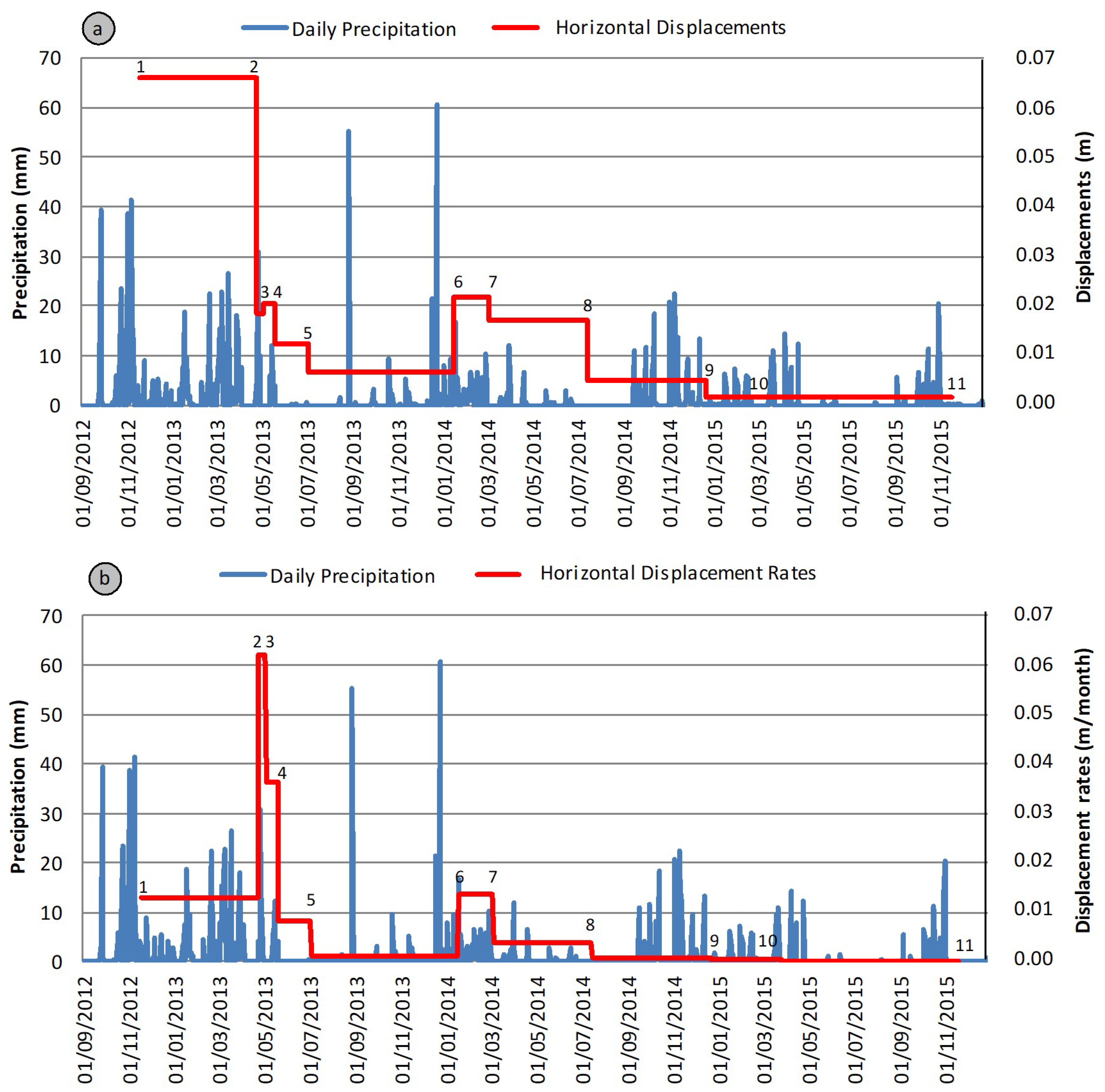
The average of the horizontal displacement rates presented a low rate of 0.13 m/month in the first period considered (19 November 2012–24 April 2013). Meanwhile, the vertical rate also registered a very low rate of descent of −0.02 m/month. The monitoring started in November 2012, after a rainy period at the beginning of the autumn. Daily precipitations reached peaks of 40 mm during some days, accumulating 120 mm in a week and 230 mm in a month. Then during the following three months the daily precipitations were less intense until March 2013, when precipitations over 30 mm occurred again, accumulating 80 mm in a week and 175 mm in a month. These two peaks could be the origin of the large displacements (0.66 m) observed in this period, although the length of the interval (more than five months) means that the rate was not so high (0.13 m/month), in the boundary between very slow and slow velocity [75].

The next period (24 April 2013–3 May 2013) recorded the maximum rates of displacement with a value of 0.62 m/month in the horizontal component and −0.06 m/month in the vertical one. These rates can be considered slow velocity rates. In this period the rainfalls presented a peak at over 40 mm at the end of April with accumulated precipitation of 55 mm in a week, 100 mm in a month and more than 300 mm in the previous 3 months. Then in the third period (3 May 2013–20 May 2013) the movement began to slow to 0.36 m/month in the horizontal and −0.03 m/month in the vertical component, which can be also catalogued as slow velocity. The daily precipitations were barely higher than 10 mm in this period, and the accumulated precipitation descended to under 25 mm in a week and 100 mm in a month.

After that, the displacement rate of the horizontal component slowed to 0.08 m/month in the fourth period (20 May 2013–4 July 2013), again being catalogued as very slow velocity. The rainfalls at the beginning of summer, which is usually dry in Mediterranean countries, were scarce and the accumulated precipitations (in a week and in a month) descended to values near 0 mm at the end of the period. In the following period (4 July 2013–17 January 2014) the horizontal and vertical displacement rates became residual, although the absolute displacements lead us to think that the landslide did not stop completely, maintaining an extremely slow velocity throughout this six-month interval. During the second half of 2013 the rainfalls were scarce in general, even in autumn and the beginning of winter, although the heaviest daily precipitations of the whole period took place on 28 August and 24 December 2013. However these isolated precipitations did not produce any landslide reactivation, taking into account that at this period the maintenance works of landslide stabilization had still not started.

A reactivation took place in the following period (17 January 2014–5 March 2014), in which the horizontal rate again reached higher values of 0.14 m/month (slow velocity), while the vertical component continued at residual values. In this period the daily precipitations were not so high, barely topping 10 mm, but the accumulated precipitations in 1 week and 1 month reached values near 40 mm and 120 mm, respectively.

After that, the movement slowed again, giving values of the horizontal rate of 0.04 m/month in the seventh period (5 March 2014–16 July 2014), catalogued again as very slow velocity. And finally, these rates dropped to values under 0.01 m/month in the last three periods (16 July 2014–23 December 2014, 23 December 2014–27 March 2015 and 27 March 2015–19 November 2015). Meanwhile the vertical rate continued at residual values during all these periods. During the second half of 2014 and 2015 the daily precipitations were scarce, barely over 20 mm, while the accumulated precipitations in a week and 1 month rarely reached 40 mm and 100 mm, respectively. Taking into account that the absolute displacements are practically null (insignificant) in the last two periods, all of these observations lead to think that the movement slowed and finally stopped as a consequence of the decreasing rainfalls and also the stabilization works of the landslide which took place between 2014 and 2016 [42].

In conclusion, the analysis by periods has allowed landslide monitoring and a detailed study of the relationship with rainfalls. In fact, rainfalls are the main triggering mechanism of the landslides all over the world [74,76] but also in the Mediterranean countries [77] and particularly in the regions near the study area [41,42,62,78]. The movement presented an intermittent character, typical of the earth flows in Mediterranean or arid climates [64,77], where the rainfalls regime shows an irregular distribution alternating between dry and wet years [79]. In this sense, the landslide could be catalogued between slow to very slow, following velocity classifications [75], and also characterized as type VII of the diachroneity classification [80] during the first periods between the autumn of 2012 and the summer of 2014. More specifically, a main activity phase of slow velocity could be described in the first months (autumn 2012–spring 2013), and after a slowing (summer 2013), a second phase of reactivation (autumn-winter 2013) was identified.

This coincides with a wet hydrologic year (2012/2013) with annual rainfall of 720 mm, and the beginning of a dry year (2013/2014) with annual rainfall around 300 mm. Finally, from summer of 2014 and autumn of 2015 the landslide stopped, probably stabilized, coinciding with a second dry year (2014/2015), in which annual rainfall was about 320 mm, and the stabilization works on the unstable slope.

Despite of this detailed study, a more systematic monitoring would be needed to establish more accurately the landslide kinematics and thus the relationships with rainfall regime and the determination of triggering thresholds. For instance, the great length of the first period has not given us better knowledge of the initial phase in which several intense rainfall episodes occurred. At the moment, although the flow-type landslides are usually related to intense but short-period rainfalls, we can establish, in a speculative way, that this earthflow needed not only intense daily or weekly precipitations (over 40 or 100 mm, respectively), but also a regime of antecedent precipitations of about 200–300 mm in a month as has been proved with other landslides in the region [41,62]. Anyway, this work demonstrates that it is possible to monitor landslides by means photogrammetric techniques based on UAV image capture. Both, the capture and processing of the images can be made in a short time allowing the monitoring of landslide kinematics and ground deformations practically in real-time. From this monitoring, prediction of next deformations and risk evaluation can be achieved.

6. Conclusions

In this study, 11 UAV flights at heights of between 40 and 100 m (GSD between 0.01 and 0.03 m) were performed in an unstable area affecting different roads. This study can be considered of ultrahigh spatial resolution and also of high temporal resolution and it has allowed the detailed description of the landslide kinematics and road deformation, both in space and time.

After the orientation of these flights using GCPs measured with DGNSS, both DSMs and orthophotographs of ultrahigh resolution (UHR) at different epochs have been obtained by means of SfM/MVS techniques. Then a set of 30 natural points, selected in the orthophotographs and the DSMs, have been extracted manually to monitor the displacements of an unstable area. The calculation of basic statistics of these points and the displacements between different epochs have allowed us to distinguish an unstable area with respect to the surrounding stable area and to analyze the landslide kinematics with a high accuracy of about 0,02 ± 0.01 m in XY and 0.04 ± 0.02 m in Z.

The unstable area has been clearly distinguished observing the distribution of SD of points coordinates at the monitoring points. Thus, the unstable points reach standard deviations of around 0.50 m in XY and 0.09 m in Z, while the stable area presents standard deviations under the significance threshold. Then the accumulated displacements in the horizontal component reached 2 m in the central part of the unstable area, decreasing gradually to the landslide margins and foot. The vertical component accumulated an average displacement around −0.23 m, corresponding to a small descent of the terrain. These conditions correspond to the foot of an earth flow, in which the deformation is higher in the central area, but in general moderate and residual.

The detailed temporal analysis of this movement has been made by means of a relatively large number of survey campaigns, which at the resolution and continuity required in this type of studies, it is only feasible with the use of UAV surveys. Thus the movement can be characterized as intermittent, with two periods of reactivation and slowing between November 2012 and the summer of 2014. The maximum displacement rate topped 0.6 m/month after several episodes of heavy rainfalls in the hydrologic year 2012/2013, with daily precipitations over 40 mm and accumulated precipitations of 120 m in a week and 300 in a month. After that, the movement slowed gradually through 2014 and finally stopped in 2015, when the rainfalls were scarce and the stabilization and reparation works of the unstable slope took place. Nevertheless, a reactivation could be detected at the beginning of 2014, coinciding with a light increase of the rainfalls at winter.

Thus, it is proved again that the use of Unmanned Aerial Vehicles (UAVs) is a useful tool for fast, very high/ultrahigh resolution and precise surveys in small areas (about 0.01 to 10 km²). Light equipment is well suited for updates and landslide monitoring, and thus for prediction or hazard and risk analysis. It allows working with intermediate scales between terrestrial techniques (global navigation satellite system—GNSS—, classic surveying, terrestrial laser scanner, terrestrial photogrammetry, geotechnical and geophysical sensors, etc.) and aerial or space surveys (conventional aerial photogrammetry, LiDAR, very high resolution satellite remote sensing and DInSAR). At this scale detailed morphological features can still be observed while allowing relatively large areas to be covered. Both data capture -including field GCPs measurement- and data processing of the images can be made in a short time. Thus the monitoring of landslide kinematics and ground deformations is addressed practically in real-time which it is crucial for the predicting of next deformations and also for risk evaluation and mitigation.

Future work will deal with advances in the capture and processing of images, regarding the reduction of ground control points using suitable equipment and applying methods of direct orientation (UAVs with RTK positioning systems). A more systematic monitoring will be required in order to obtain better knowledge of landslide dynamics that could be facilitated with a reduction of time and costs derived of more efficient capture and processing techniques.

Moreover, techniques for the automatic detection of surface motions based on expert classification techniques from DSMs and images should be explored. Finally, other sensors can be incorporated into both the spectral domain (i.e., near and thermal infrared sensors) and the geometric domain (LiDAR and RADAR).

References

- Arbanas, S.M.; Arbanas, Ž. Landslide mapping and monitoring: Review of conventional and advanced techniques. In Proceedings of the 4th Symposium of Macedonian Association for Geotechnics, Struga, Macedonia, 25–28 June 2014; pp. 57–72. [Google Scholar]
- Savvaidis, P.D. Existing landslide monitoring systems and techniques. In Stars to Earth and Culture, in Honor of the Memory of Professor Alexandros Tsioumis; Dermanis, A., Ed.; Ziti Publications: Thessaloniki, Greece, 2003; pp. 242–258. [Google Scholar]
- Metternicht, G.; Hurni, L.; Gogu, R. Remote sensing of landslides: An analysis of the potential contribution to geo-spatial systems for hazard assessment in mountainous environments. Remote Sens. Environ. 2005, 98, 284–303. [Google Scholar] [CrossRef]
- Tofani, V.; Hong, Y.; Singhroy, V. Introduction: Remote Sensing Techniques for Landslide Mapping and Monitoring. In Landslide Science for a Safer Geoenvironment; Sassa, K., Canuti, P., Yin, Y., Eds.; Springer International Publishing: Cham, Switzerland, 2014; Volume 2, pp. 301–303. [Google Scholar]
- Xhao, C.; Lu, Z. Remote Sensing of Landslides—A Review. Remote Sens. 2018, 10, 279. [Google Scholar]
- Walstra, J.; Chandler, J.H.; Dixon, N.; Dijkstra, T.A. Time for change—Quantifying land-slide evolution using historical aerial photographs and modern photogrammetric methods. Int. Arch. Photogramm. Remote Sens. Spat. Inf. Sci. 2004, XXXV, 475–480. [Google Scholar]
- Fernández, T.; Pérez, J.L.; Colomo, C.; Cardenal, J.; Delgado, J.; Palenzuela, J.A.; Irigaray, C.; Chacón, J. Assessment of the Evolution of a Landslide Using Digital Photogrammetry and LiDAR Techniques in the Alpujarras Region (Granada, Southeastern Spain). Geosciences 2017, 7, 32. [Google Scholar] [CrossRef]
- Angeli, M.G.; Pasuto, A.; Silvano, S. A critical review of landslide monitoring experiences. Eng. Geol. 2000, 55, 133–147. [Google Scholar] [CrossRef]
- Gili, J.A.; Corominas, J.; Rius, J. Using Global Positioning System techniques in landslide monitoring. Eng. Geol. 2000, 55, 167–192. [Google Scholar] [CrossRef]
- Mikkelsen, P.E. Field instrumentation. In Landslides—Investigation and Mitigation; Transportation Research Board Special Report; Turner, A.K., Schuster, R.L., Eds.; National Academy Press: Washington, DC, USA, 1996; Volume 247, pp. 278–316. [Google Scholar]
- Abramson, L.W.; Lee, T.S.; Sharma, S.; Boyce, G.M. Slope Stability and Stabilization Methods; John Wiley & Sons: New York, NY, USA, 2002. [Google Scholar]
- Gao, W.; He, T.Y. Displacement prediction in geotechnical engineering based on evolutionary neural network. Geomech. Eng. 2017, 13, 845–860. [Google Scholar]
- Reichenbach, P.; Rossi, M.; Malamud, B.D.; Mihir, M.; Guzzetti, F. A review of statistically-based landslide susceptibility models. Earth Sci. Rev. 2018, 180, 60–91. [Google Scholar] [CrossRef]
- Chacón, J.; El Hamdouni, R.; Irigaray, C.; Fernández, T. Engineering geology maps: Landslides and GIS. Bull. Eng. Geol. Environ. 2006, 65, 341–411. [Google Scholar] [CrossRef]
- Brückl, E.; Brunner, F.K.; Kraus, K. Kinematics of a deep-seated landslide derived from photogrammetric, GPS and geophysical data. Eng. Geol. 2006, 88, 149–159. [Google Scholar] [CrossRef]
- Cardenal, J.; Delgado, J.; Mata, E.; González, A.; Olague, I. Use of historical flight for landslide monitoring. In Proceedings of the Spatial Accuracy 2006, Lisbonne, Portugal, 5–7 July 2006; pp. 129–138. [Google Scholar]
- Dewitte, O.; Jasselette, J.C.; Cornet, Y.; Van Den Eeckhaut, M.; Collignon, A.; Poesen, J.; Demoulin, A. Tracking landslide displacement by multi-temporal DTMs: A combined aerial stereophotogrammetric and LiDAR approach in Belgium. Eng. Geol. 2008, 99, 11–22. [Google Scholar] [CrossRef]
- Kasperski, J.; Delacourt, C.; Allemand, P.; Potherat, P. Evolution of the Sedrun landslide (Graubünden, Switzerland) with ortho-rectified air images. Bull. Eng. Geol. Environ. 2010, 69, 421–430. [Google Scholar] [CrossRef]
- Prokešová, R.; Kardoš, M.; Medveďová, A. Landslide dynamics from high-resolution aerial photographs: A case study from W Carpathians, Slovakia. Geomorphology 2010, 115, 90–101. [Google Scholar] [CrossRef]
- Fabris, M.; Menin, A.; Achilli, V. Landslide displacement estimation by archival digital photogrammetry. Ital. J. Remote Sens. 2011, 43, 23–30. [Google Scholar] [CrossRef]
- Kraus, K. Photogrammetry: Geometry from Images and Laser Scans; Walter de Gruyter: Berlin, Germany, 2007. [Google Scholar]
- Hartley, R.; Zisserman, A. Multiple View Geometry in Computer Vision; Cambridge University Press: Cambridge, UK, 2004; p. 655. [Google Scholar]
- Eltner, A.; Kaiser, A.; Castillo, C.; Rock, G.; Neugirg, F.; Abellán, A. Image-based surface reconstruction in geomorphometry—Merits, limits and developments. Earth Surf. Dyn. 2016, 4, 359–389. [Google Scholar] [CrossRef]
- AGISOFT. Agisoft PhotoScan. Available online: https://www.agisoft.com/ (accessed on 31 March 2019).
- PIX4D. Professional Photogrammetry and Drone Mapping Software. Available online: https://www.pix4d.com/ (accessed on 31 March 2019).
- González-Aguilera, D.; López-Fernández, L.; Rodriguez-Gonzalvez, P.; Guerrero, D.; Hernandez-Lopez, D.; Remondino, F.; Menna, F.; Nocerino, E.; Toschi, I.; Ballabeni, A.; et al. Development of an all-purpose free photogrammetric tool. Int. Arch. Photogramm. Remote Sens. Spat. Inf. Sci. 2016, XLI-B6, 31–38. [Google Scholar] [CrossRef]
- Wu, C. VisualSFM: A Visual Structure from Motion System. Available online: http://ccwu.me/vsfm/ (accessed on 31 March 2019).
- Yang, Z.; Lan, H.; Gao, X.; Li, L.; Meng, Y.; Wu, Y. Urgent landslide susceptibility assessment in the 2013 Lushan earthquake-impacted area, Sichuan Province, China. Nat. Hazards 2015, 75, 2467–2487. [Google Scholar] [CrossRef]
- Fan, X.; Scaringi, G.; Xu, Q.; Zhan, W.; Dai, L.; Li, Y.; Pei, X.; Yang, Q.; Huang, R. Coseismic landslides triggered by the 8th August 2017 Ms 7.0 Jiuzhaigou earthquake (Sichuan, China): Factors controlling their spatial distribution and implications for the seismogenic blind fault identification. Landslides 2018, 15, 967–983. [Google Scholar] [CrossRef]
- Yeh, M.L.; Hsiao, Y.C.; Chen, Y.H.; Chung, J.C. A study on Unmanned Aerial Vehicle applied to acquire terrain information of landslide. In Proceedings of the 32 Asian Conference Remote Sensing, Taipei, Taiwan, 3–7 October 2011; Volume 3, pp. 2210–2215. [Google Scholar]
- Liu, C.; Chen, P.; Matsuo, T.; Chen, C. Rapidly responding to landslides and debris flow events using a low cost unmanned aerial vehicle. J. Appl. Remote Sens. 2015, 9, 096016. [Google Scholar] [CrossRef]
- Huang, Y.; Yi, S.; Lia, Z.; Shao, S.; Qin, X. Design of highway landslide warning and emergency response systems based on UAV. In Proceedings of the 17th China Conference on Remote Sensing, Hangzhou, China, 27–31 August 2010; SPIE: Bellingham, WA, USA, 2011; Volume 8203, 820317. [Google Scholar]
- Tahar, K.N.; Ahmad, A.; Akib, W.A.A.W.M.; Mohd, W.M.N.W. Unmanned Aerial Vehicle Photogrammetric Results Using Different Real Time Kinematic Global Positioning System Approaches. In Developments in Multidimensional Spatial Data Models; Lecture Notes in Geoinformation and Cartography; Raman, A.A., Bogulawski, P., Gold, C., Said, M.N., Eds.; Springer: Berlin/Heidelberg, Germany, 2013; pp. 123–134. [Google Scholar]
- Warrick, J.A.; Ritchie, A.C.; Schmidt, K.M.; Reid, M.E.; Logan, J. Characterizing the catastrophic 2017 Mud Creek landslide, California, using repeat structure-from-motion (SfM) photogrammetry. Landslides 2019, 16, 1201–1219. [Google Scholar] [CrossRef]
- Shi, B.; Liu, C. UAV for Landslide Mapping and Deformation Analysis. In Proceedings of the International Conference on Intelligent Earth Observing and Applications, Guilin, China, 23–24 October 2015; SPIE: Bellingham, WA, USA, 2015; Volume 9808, 98080P. [Google Scholar]
- Hsieh, Y.C.; Chan, Y.; Hu, J. Digital elevation model differencing and error estimation from multiple sources: A case study from the Meiyuan Shan landslide in Taiwan. Remote Sens. 2016, 8, 199. [Google Scholar] [CrossRef]
- Liu, C.; Li, W.; Lei, W.; Liu, L.; Hu, H. Architecture planning and geo-disasters assessment mapping of landslide by using airborne LiDAR data and UAV images. In Proceedings of the International Symposium on Lidar and Radar Mapping 2011: Technologies and Applications, Nanjing, China, 26–29 May 2011; SPIE: Bellingham, WA, USA, 2011; Volume 8286, 82861Q. [Google Scholar]
- Niethammer, U.; James, M.R.; Rothmund, S.; Travelletti, J.; Joswig, M. UAV-based remote sensing of the Super-Sauze landslide: Evaluation and results. Eng. Geol. 2012, 128, 2–11. [Google Scholar] [CrossRef]
- Stumpf, A.; Malet, J.P.; Kerle, N.; Niethammer, U.; Rothmund, S. Image-based mapping of surface fissures for the investigation of landslide dynamics. Geomorphology 2013, 186, 12–27. [Google Scholar] [CrossRef] [Green Version]
- Turner, D.; Lucieer, A.; de Jong, S.M. Time series analysis of landslide dynamics using an Unmanned Aerial Vehicle (UAV). Remote Sens. 2015, 7, 1736–1757. [Google Scholar] [CrossRef]
- Fernández, T.; Pérez, J.L.; Cardenal, F.J.; López, A.; Gómez, J.M.; Colomo, C.; Sánchez, M.; Delgado, J. Use of a light UAV and photogrammetric techniques to study the evolution of a landslide. Int. Arch. Photogramm. Remote Sens. Spat. Inf. Sci. 2015, XL-3-W3, 241–248. [Google Scholar]
- Fernández, T.; Pérez, J.L.; Cardenal, F.J.; Gómez, J.M.; Colomo, C.; Delgado, J. Analysis of landslide evolution affecting olive groves using UAV and photogrammetric techniques. Remote Sens. 2016, 8, 837. [Google Scholar] [CrossRef]
- Peterman, V. Landslide activity monitoring with the help of unmanned aerial vehicle. Int. Arch. Photogramm. Remote Sens. Spat. Inf. Sci. 2015, XL-1/W4, 215–218. [Google Scholar] [CrossRef]
- Daakir, M.; Pierrot-Deseilligny, M.; Bosser, P.; Pichard, F.; Thom, C. UAV onboard photogrammetry and GPS positioning for earthworks. Int. Arch. Photogramm. Remote Sens. Spat. Inf. Sci. 2015, XL-3/W3, 293–298. [Google Scholar] [CrossRef]
- Al-Rawabdeh, A.; He, F.; Moussa, A.; El-Sheimy, N.; Habib, A. Using an unmanned aerial vehicle-based digital imaging system to derive a 3D point cloud for landslide scarp recognition. Remote Sens. 2016, 8, 95. [Google Scholar] [CrossRef]
- Lindner, G.; Schraml, K.; Mansberger, R.; Hübl, J. UAV monitoring and documentation of a large landslide. Appl. Geomat. 2016, 8, 1–11. [Google Scholar] [CrossRef]
- James, M.R.; Robson, S.; d’Oleire-Oltmanns, S.; Niethammerd, U. Optimising UAV topographic surveys processed with structure-from-motion: Ground control quality, quantity and bundle adjustment. Geomorphology 2017, 280, 51–66. [Google Scholar] [CrossRef] [Green Version]
- Dang, K.; Sassa, K.; Fukuoka, H.; Sakai, N.; Sato, Y.; Takara, K.; Quang, L.H.; Loi, D.H.; Tien, P.V.; Ha, N.D. Mechanism of two rapid and long-runout landslides in the 16 April 2016 Kumamoto earthquake using a ring-shear apparatus and computer simulation (LS-RAPID). Landslides 2016, 13, 1525–1534. [Google Scholar] [CrossRef]
- Mozas-Calvache, A.T.; Pérez-García, J.L.; Fernández, T. Monitoring of landslide displacements using UAS and control methods based on lines. Landslides 2017, 14, 2115–2128. [Google Scholar] [CrossRef]
- Peternel, T.; Kumelj, S.; Oštir, K.; Komac, M. Monitoring the Potoška planina landslide (NW Slovenia) using UAV photogrammetry and tachymetric measurements. Landslides 2017, 14, 395–406. [Google Scholar] [CrossRef]
- Balek, J.; Blahůt, J. A critical evaluation of the use of an inexpensive camera mounted on a recreational unmanned aerial vehicle as a tool for landslide research. Landslides 2017, 14, 1217–1224. [Google Scholar] [CrossRef]
- Peppa, M.V.; Mills, J.P.; Moore, P.; Miller, P.E.; Chambers, J.E. Brief communication: Landslide motion from cross correlation of UAV-derived morphological attributes. Nat. Hazards Earth Syst. Sci. 2017, 17, 2143–2150. [Google Scholar] [CrossRef] [Green Version]
- Peppa, M.V.; Mills, J.P.; Moore, P.; Miller, P.E.; Chambers, J.E. Automated co-registration and calibration in SfM photogrammetry for landslide change detection. Earth Surf. Process. Landforms 2019, 44, 287–303. [Google Scholar] [CrossRef]
- Hu, S.; Qiu, H.; Wang, X.; Gao, Y.; Wang, N.; Wu, J.; Yang, D.; Cao, M. Acquiring high-resolution topography and performing spatial analysis of loess landslides by using low-cost UAVs. Landslides 2018, 15, 593–612. [Google Scholar] [CrossRef]
- Rossi, G.; Tanteri, L.; Tofani, V.; Vannocci, P.; Moretti, S.; Casagli, N. Multitemporal UAV surveys for landslide mapping and characterization. Landslides 2018, 15, 1045–1052. [Google Scholar] [CrossRef] [Green Version]
- Fan, X.; Xu, Q.; Scaringi, G.; Zheng, G.; Huang, R.; Dai, L.; Ju, Y. The “long” runout rock avalanche in Pusa, China, on August 28, 2017: A preliminary report. Landslides 2019, 16, 139–154. [Google Scholar] [CrossRef]
- Ma, S.; Xu, C.; Shao, X.; Zhang, P.; Liang, X.; Tian, Y. Geometric and kinematic features of a landslide in Mabian Sichuan, China, derived from UAV photography. Landslides 2019, 16, 373–381. [Google Scholar] [CrossRef]
- Stöcker, C.; Nex, F.; Koeva, M.; Gerke, M. Quality assessment of combined IMU/GNSS data for direct georeferencing in the context of UAV-based mapping. Int. Arch. Photogramm. Remote Sens. Spat. Inf. Sci. 2017, 42, 355–361. [Google Scholar] [CrossRef]
- Forlani, G.; Dall’Asta, E.; Diotri, F.; Cella, U.M.D.; Roncella, R.; Santise, M. Quality assessment of DSMs produced from UAV flights georeferenced with onboard RTK positioning. Remote Sens. 2018, 10, 311. [Google Scholar] [CrossRef]
- Rabah, M.; Basiouny, M.; Ghanem, E.; Elhadary, A. Using RTK and VRS in direct geo-referencing of the UAV imagery. NRIAG J. Astron. Geophys. 2018, 7, 220–226. [Google Scholar] [CrossRef] [Green Version]
- Colomo, C.M.; Pérez-García, J.L.; Gómez-López, J.; Fernández, T. Análisis de la actividad de deslizamientos mediante técnicas de LiDAR y fotogrametría en el entorno de la autovía A-44 (Jaén). In Proceedings of the IX Simposio Nacional Sobre Laderas y Taludes Inestables, Santander, Spain, 27–30 June 2017; Volume 1, pp. 492–503. [Google Scholar]
- Carpena, R.L.; Mellado, I.; Moya, F.; Colomo, C.; Bédmar, P.; Calero, J.; Pérez, A.; Fernández, T.; Sánchez-Gómez, M.; Tovas, J. Análisis de riesgos asociados a las infraestructuras viarias de la Diputación Provincial de Jaén. In Proceedings of the IX Simposio Nacional Sobre Laderas y Taludes Inestables, Santander, Spain, 27–30 June 2017; Volume 1, pp. 335–346. [Google Scholar]
- Varnes, D.J. Slope movement, types and processes. In Landslides: Analysis and Control; Transportation Research Board Special Report; Schuster, R.L., Krizek, R.J., Eds.; National Academy of Sciences: Washington, DC, USA, 1978; Volume 176, pp. 12–33. [Google Scholar]
- Hungr, O.; Leroueil, S.; Picarelli, L. The Varnes classification of landslide types, an update. Landslides 2014, 11, 167–194. [Google Scholar] [CrossRef]
- Roldán, F.J.; Lupiani, E.; Jerez, L. Mapa Geológico de España, Escala 1:50.000, Mapa y Memoria Explicativa; Instituto Geológico Nacional: Madrid, Spain, 1988. [Google Scholar]
- Pérez-Valera, F.; Sánchez-Gómez, M.; Pérez-López, A.; Pérez-Valera, L.A. An evaporite-bearing accretionary complex in the northern front of the Betic-Rif orogeny. Tectonics 2017, 36, 1006–1036. [Google Scholar] [CrossRef]
- Navarro, V.; Ruiz-Ortiz, P.A.; Molina, J.M. Birth and demise of a Middle Jurassic isolated shallow-marine carbonate platform on a tilted fault block: Example from the Southern Iberian continental palaeomargin. Sediment. Geol. 2012, 269, 37–57. [Google Scholar] [CrossRef]
- Sánchez-Gómez, M.; Peláez, J.A.; García-Tortosa, F.J.; Torcal, F.; Soler, P.; Ureña, M.A. Aproximación geológica, geofísica y geomorfológica a la actividad tectónica en el valle del alto Guadalquivir. In Proceedings of the 6th Asamblea Hispano Portuguesa de Geodesia y Geofísica, Tomar, Portugal, 5–8 September 2008. [Google Scholar]
- González-Díez, A.; Fernández-Maroto, G.; Doughty, M.W.; Díaz de Terán, J.R.; Bruschi, V.; Cardenal, J.; Pérez, J.L.; Mata, E.; Delgado, J. Development of a methodological approach for the accurate measurement of slope changes due to landslides, using digital photogrammetry. Landslides 2014, 11, 615–628. [Google Scholar] [CrossRef]
- AscTec. AscTec Falcon 8 + AscTec Trinity. Ascending Technologies. Available online: http://www.asctec.de/downloads/public/F8_AscTec-Falcon-8-AscTec-Trinity_safety-data-sheet.pdf (accessed on 31 March 2019).
- QGIS. A Free and Open Source Geographic Information System. Available online: https://www.qgis.org/en/site/ (accessed on 31 March 2019).
- IAEG. Commission on Landslides. Suggested nomenclature for landslides. Bull. IAEG 1990, 41, 13–16. [Google Scholar]
- Hutchinson, J.N. General Report: Morphological and Geotechnical Parameters of Landslides in Relation to Geology and Hydrogeology. In Proceedings of the 5th International Symposium on Landslides, Lausanne, Switzerland, 10–15 July 1988. [Google Scholar]
- Crozier, M.J. Techniques for the morphometric analysis of landslips. Z. Geomorphol. 1973, 17, 78–101. [Google Scholar]
- International Union of Geological Sciences Working Group on Landslides. A suggested method for describing the rate of movement of a landslide. Bull. Eng. Geol. Environ. 1995, 52, 75–78. [Google Scholar]
- Finlay, P.J.; Fell, R.; Maguire, P.K. The relationship between the probability of landslide occurrence and rainfall. Can. Geotech. J. 1997, 34, 811–824. [Google Scholar] [CrossRef]
- Guzzeti, F. Landslide hazard assessment and risk evaluation: Limits and prospectives. In Proceedings of the 4th EGS Plinius Conference, Mallorca, Spain, 2–4 October 2002. [Google Scholar]
- Irigaray, C.; Lamas, F.; El Hamdouni, R.; Fernández, T.; Chacón, J. The importance of the precipitation and the susceptibility of the slopes for the triggering of landslides along the roads. Nat. Hazards 2000, 21, 65–81. [Google Scholar] [CrossRef]
- Chacón, J.; Irigaray, C.; El Hamdouni, R.; Jiménez, J.D. Diachroneity of landslides. In Geologically Active; Williams, A.L., Pinches, G.M., Chin, C.Y., McMorran, T.J., Massey, C.I., Eds.; Taylor & Francis Group: London, UK, 2010; pp. 999–1006. [Google Scholar]
- Trigo, R.M.; Pozo, D.; Timothy, C.; Osborn, J.; Castro, Y.; Gámiz, S.; Esteban, M.J. North Atlantic Oscillation influence on precipitation, river flow and water resources in the Iberian Peninsula. Int. J. Climatol. 2004, 24, 925–994. [Google Scholar] [CrossRef]
Figure 1.
Geographical location and geological setting: (a) Geographical location; (b) Landslide and study area; (c) Geological setting (taken from the Geological Map of Spain at scale 1:50,000, [65]). Coordinates are in ETRS89-UTM-30N.
Figure 2.
(a) Photorealistic reconstructions of the landslide foot with the roads affected: (a): 24 April 2013 frontal view; (b): 24 April 2013 lateral view; (c): 5 March 2014 frontal view; (d): 5 March 2014 lateral view; (e) 19 November 2015 frontal view; (f): 19 November 2015 lateral view (it can be observed the drainage wells and the retaining wall).
Figure 3.
Methodology flow chart.
Figure 4.
Landslide and affected roads. (a) surveyed area (red rectangle) on affected roads and access to highway at the landslide foot; (b) Mission planning and location of trigger points for the low height flights; (c) Mission planning and photo footprints of low height flights; (d) Main landslide affecting the slope (yellow dash line) and surveyed area (red rectangle); (e) Mission planning and location of trigger points for the general flights for the slope monitoring [42]; (f) photo footprints of the strips used in this paper from the general flights of the slope (19 November 2012; 16 July 2014). Coordinates are in ETRS89-UTM-30N.
Figure 5.
Examples of targets for GCP and CHK points as seen from 40 m flying height. (a) White circles on black background (inside the white circle there is small black circle for accurate image measurement) printed on PVC foam board. (b) Circle/sector target sprayed on the ground with reflective red paint and a cardboard template. (c) Natural and well defined natural points (road reflective markers and corners on road surface markings).
Figure 6.
Standard deviation of monitoring points. Horizontal component: (a) Map; (c) Histogram; Vertical component: (b) Map; (d) Histogram. Both maps are based on the orthophotograph of 2013/05/03. Coordinates are in ETRS89-UTM-30N.
Figure 7.
Maps of displacements of monitoring points for the different periods. (a) 19 November 2012–24 April 2013; (b) 24 April 2013–3 May 2013; (c) 3 May 2013–20 May 2013; (d) 20 May 2013–4 July 2013; (e) 4 July 2013–17 January 2014; (f) 17 January 2014–5 March 2014; (g) 5 March 2014–16 July 2014; (h) 16 July 2014–23 December 2014; (i) 23 December 2014–27 March 2015; (j) 27 March 2015–19 November 2015); (k,l) 19 November 2012–19 November 2015) (total period). Orthophotographs correspond to the first date, except (l) that corresponds to the end date. Coordinates are in ETRS89-UTM-30N.
Figure 8.
Relationships between the horizontal displacements and the rainfalls in the study period considered. (a) Displacements and rainfalls; (b) Displacements rates and rainfalls. Numbers indicate the measurement epoch (1 to 11).