Gravity Field Model Determination Based on GOCE Satellite Point-Wise Accelerations Estimated from Onboard Carrier Phase Observations

Abstract

GPS-based, satellite-to-satellite tracking observations have been extensively used to elaborate the long-scale features of the Earth’s gravity field from dedicated satellite gravity missions. We proposed compiling a satellite gravity field model from Gravity Field and Steady-State Ocean Circulation Explorer (GOCE) satellite accelerations directly estimated from the onboard GPS data using the point-wise acceleration approach, known as the carrier phase differentiation method. First, we composed the phase accelerations from the onboard carrier phase observations based on the sixth-order seven-point differentiator, which can eliminate the carrier phase ambiguity for Low Earth Orbiter (LEO). Next, the three-dimensional (3D) accelerations of the GOCE satellite were estimated from the derived phase accelerations as well as GPS satellite ephemeris and precise clock products. Finally, a global gravity field model up to the degree and order (d/o) 130 was compiled from the 71 days and nearly 2.5 years of 3D satellite accelerations. We also recovered three gravity field models up to d/o 130 from the accelerations derived by differentiating the kinematic orbits of European Space Agency (ESA), Graz, and School of Geodesy and Geomatics (SGG), which was the orbit differentiation method. We analyzed the accuracies of the derived accelerations and the recovered gravity field models based on the carrier phase differentiation method and orbit differentiation method in time, frequency, and spatial domain. The results showed that the carrier phase derived acceleration observations had better accuracy than those derived from kinematic orbits. The accuracy of the recovered gravity field model based on the carrier phase differentiation method using 2.5 years observations was higher than that of the orbit differentiation solutions for degrees greater than 70, and worse than Graz-orbit solution for degrees less than 70. The cumulative geoid height errors of carrier phase, ESA-orbit, and Graz-orbit solutions up to degree and order 130 were 17.70cm, 21.43 cm, and 22.11 cm, respectively.

1. Introduction

The modeling of Earth’s gravity field is an essential task in the physical geodesy, and the constructed gravity information can be used for the fields of soild geophysics, oceanography, geodesy, and glaciology [1]. Beginning in the year 2000, several dedicated satellite gravimetry missions, such as the CHAllenging Minisatellite Payload (CHAMP), Gravity Recovery And Climate Experiment (GRACE), and Gravity field and steady-state Ocean Circulation Explorer (GOCE), have significantly improved the accuracy of the static gravity field and its temporal variations by several orders of magnitude [2,3,4]. Although these missions were carried out with different measurement principles, they had a common feature: all were equipped with global positioning system (GPS) receivers to realize the concept known as satellite-to-satellite tracking in high-low mode (SST-hl). SST-hl is a highly sophisticated technique to map the long-wavelength spectrum of the gravity field [5,6,7].

There are four methods for gravity field recovery that use SST-hl observations: celestial mechanics, energy balance, short-arc, and acceleration methods [8]. According to the types of differentiated acceleration, two acceleration methods exist: the average acceleration method and point-wise acceleration method [9]. Baur et al. [8] and Pail et al. [10] compared the different methods for modeling gravity field models with the GOCE SST-hl data and pointed out that, with the exception of the energy balance method, the other three methods had a comparable performance. The celestial mechanics approach is confronted with a large computational effort due to the integration of the variation equations and a nonlinear system of equations; in the case of the energy balance method, space gravity spectroscopy information is exclusively scalar and not available in all three directions [11,12,13]. The acceleration method is based on Newton’s equation of motion, which balances the gravitational vector with satellite accelerations in the inertial reference frame [14,15]. The principle of acceleration approach is simple and has been successfully applied to CHAMP, GRACE, and GOCE SST-hl data analysis [14,15,16,17,18,19].

The key to recovering the gravity model by the acceleration method is to estimate the satellite accelerations with a high degree of precision. Several approaches have been used to estimate the GPS-based acceleration including orbit differentiation, Doppler differentiation, and carrier phase differentiation approaches [20]. The most commonly used method is performed by double time-differentiating successive trajectories of the moving satellite, also known as the orbit differentiation algorithm. A major drawback to this method is that the accuracy of the differentiated accelerations is strongly dependent on the position precision; an increase or decrease in the number of visible satellites can lead to discontinuities [21]. Another method is the Doppler measurement, which can be used afterward to obtain the satellite’s velocity before the satellite accelerations are computed by the first-order derivative of the satellite’s velocity. One shortcoming is that the raw Doppler observables may be heavily contaminated by measurement noises [22]. An alternative method is to numerically differentiate the GPS carrier phase observations then obtain both the range rate and range acceleration, which is called the carrier phase differentiation method. This method has been successfully applied in airborne gravimetry [23,24] and satellite gravimetry [25]. The most prominent advantage of this approach is the avoidance of the cycle ambiguity problem and the elimination of systematic errors (e.g., hardware delays from the receiver and GPS satellites) that are common to adjacent epochs [23,25].

Guo et al. [25] adopted the average acceleration approach to recover the gravity field model from satellite accelerations derived from onboard GPS phase measurements. It was shown that the noise of the accelerations derived by the carrier phase differentiation method was lower than that derived by the orbit differentiation method in all three components, especially in the cross-track component, which showed an improvement of about 20%. Thus, the recovered gravity field based on the carrier phase differentiation accelerations had a slightly higher accuracy when compared with the solution based on the orbit differentiation method. It should be noted that Guo et al. [25] estimated the average satellite accelerations in two steps: first, the position differences epoch by epoch were derived directly from the GPS carrier phase measurements; the average satellite accelerations were then obtained with the position differences.

In this study, we proposed to recover the gravity field model based on the point-wise accelerations of the GOCE satellite estimated by the carrier phase differentiation method from the onboard carrier phase observations. This idea has not yet been addressed and differs from the average acceleration approach used for gravity field modeling and the approach of estimating the satellite accelerations in Guo et al. [25]. The paper is organized as follows. 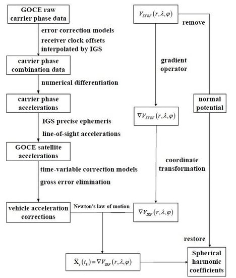Section 2 describes the functional models of satellite acceleration and gravity field determination. Section 3 shows the experimental results. Section 4 discusses the findings of this research, and Section 5 presents our conclusions.

2. Methods

In this paper, the point-wise acceleration approach was applied to recover the gravity field model from the 3D satellite positions, which were computed based on either the carrier phase differentiation method or orbit differentiation algorithm. The functional models for the satellite acceleration determination are given in Section 2.1, and the point-wise acceleration approach for recovering the gravity field model is briefly summarized in Section 2.2.

2.1. Functional Models for the Determination of the Satellite Acceleration

2.1.1. Numerical Differentiation Method

The numerical differentiation approach is often used to derive the second order derivative from the time series {z(t)}; a functional model with constant coefficients is fitted to the time series and is subsequently differentiated analytically to obtain its derivatives. There are numerous numerical differentiators that could be used in this approach, including polynomial interpolation, Newton–Gregory differentiation, and Taylor–MacLaurin differentiation [26]. With reference to the analysis of the computational efficiency and performance in Baur et al. [8], we adopted the sixth-order seven-point polynomial fitting in this article. The basic formula for polynomial interpolation depending on the time difference $\tau$ is expressed as [26]:

$$z{\left(t_0+{\tau }_i\right)}_N={\displaystyle \sum _{j=0}^N{c}_j{\tau }_i^j},{\tau }_i=\left(i-\left[\frac{M}{2}\right]\right)\Delta t$$

(1)

where $z\left(t_0+{\tau }_i\right)$ is the arbitrary time series; i is the index of interpolated points; $t_0$ is the time at which the polynomial is evaluated; ${\tau }_i$ is the time difference between $t_0$ and the actual data point; $M$ is the total number of data points used for the interpolation; $N$ is the degree of the polynomial; $\Delta t$ is the sampling interval; and $c_j$ is the polynomial coefficient.

The polynomial was fitted to numbers of neighboring points along the satellite track and then the polynomial coefficients were estimated through a classical least squares [18,26]. Due to polynomial oscillations at the interval boundaries, the polynomial was evaluated at the central point. Finally, we respectively differentiated Equation (1) once and twice, which provided the following formula:

$$\begin{array}{l}\dot{z}\left(t_0\right)={\mathrm{g}}_{}^T·z\\ \ddot{z}\left(t_0\right)=h_{}^T·z\end{array}$$

(2)

where $\dot{z}\left(t_0\right),\ddot{z}\left(t_0\right)$ are the first and second derivatives of the time series; g and h are the differentiation operator with the constant coefficients corresponding to the sixth-order seven-point polynomial, which are shown in the following:

$$\begin{array}{l}{g}^T=\left[\begin{array}{ccccccc}\frac{-1}{60\Delta t}& \frac{3}{20\Delta t}& \frac{-3}{4\Delta t}& 0& \frac{3}{4\Delta t}& \frac{-3}{20\Delta t}& \frac{1}{60\Delta t}\end{array}\right]\\ h^T=\left[\begin{array}{ccccccc}\frac{1}{90\Delta t^2}& \frac{-3}{20\Delta t^2}& \frac{3}{2\Delta t^2}& \frac{-49}{18\Delta t^2}& \frac{3}{2\Delta t^2}& \frac{-3}{20\Delta t^2}& \frac{1}{90\Delta t^2}\end{array}\right]\end{array}$$

(3)

2.1.2. Carrier Phase Differentiation Method

The ionosphere-free carrier phase combination observation between the GPS satellite and LEO satellite receiver is given as follows [21]:

$${\phi }_r^S={\rho }_r^S+c\left(d{t}_r-d{t}^S\right)+re{l}_r^S+N_r^S+{\omega }_r^S+{\epsilon }_r^S$$

(4)

where ${\phi }_r^S$ is the ionosphere-free carrier phase combination measurement; ${\rho }_r^S$ is the geometric range between the GPS satellite and the LEO satellite receiver antenna; $d{t}_r$ and $d{t}^S$ are the LEO satellite and GPS satellite clock offsets, respectively; $re{l}_r^S$ is the relativistic correction; $N_r^S$ is the carrier phase ambiguity; ${\omega }_r^S$ is the wind-up effect; and ${\epsilon }_r^S$ is the remaining unidentifiable noise.

The data pre-processing of raw carrier phase observations focused on the error corrections in Equation (4). The accurate error corrections ($re{l}_r^S$ and ${\omega }_r^S$) terms were modeled referring to Montenbruck et al. [27] and the satellite receiver clock offsets $d{t}^S$ were interpolated with GPS precise clock products released by International GNSS Service(IGS) [28]. After pre-processing the data, we could construct an item ${\widehat{\phi }}_r^S={\phi }_r^S+cd{t}^S-re{l}_r^S-{\omega }_r^S$, and introduce it into Equation (4). We have:

$${\widehat{\phi }}_r^S={\rho }_r^S+cd{t}_r+N_r^S+{\epsilon }_r^S$$

(5)

Differentiating Equation (5) yields [24]:

$${\dot{\widehat{\phi }}}_r^S={\dot{\rho }}_r^S+cd{\dot{t}}_r+{\dot{N}}_r^S+{\dot{\epsilon }}_r^S$$

(6)

Given that ${\dot{N}}_r^S=0$ when no cycle slip occurs with ${\dot{\epsilon }}_r^S$ omitted, we have:

$${\dot{\widehat{\phi }}}_r^S={\dot{\rho }}_r^S+cd{\dot{t}}_r$$

(7)

Differentiating Equation (7) then gives:

$${\ddot{\widehat{\phi }}}_r^S={\ddot{\rho }}_r^S+cd{\ddot{t}}_r$$

(8)

According to the inter-satellite geometric relationship between the GPS satellite and LEO satellite [29], the equations of the LEO’s satellite velocity and acceleration are represented as [24]:

$$\{\begin{array}{l}{\dot{\rho }}_r^S-{\mathit{e}}_{\mathit{r}}^{\mathit{S}}·{\dot{\mathit{x}}}^{\mathit{S}}=-{\mathit{e}}_{\mathit{r}}^{\mathit{S}}·{\dot{\mathit{x}}}_{\mathit{r}}\\ {\ddot{\rho }}_r^S-{\mathit{e}}_{\mathit{r}}^{\mathit{S}}·{\ddot{\mathit{x}}}^{\mathit{S}}-\frac{1}{{\rho }_r^S}\left[{\left|{\dot{\mathit{x}}}_{\mathit{r}}^{\mathit{S}}\right|}^2-{\left({\dot{\rho }}_r^S\right)}^2\right]=-{\mathit{e}}_{\mathit{r}}^{\mathit{S}}·{\ddot{\mathit{x}}}_{\mathit{r}}\end{array}$$

(9)

where ${\mathit{e}}_{\mathit{r}}^{\mathit{S}}$ is the unit direction vector between the GPS satellite and LEO satellite receiver; ${\dot{\mathit{x}}}^{\mathit{S}}$ and ${\ddot{\mathit{x}}}^{\mathit{S}}$ are the GPS satellite velocity and acceleration; and ${\dot{\mathit{x}}}_{\mathit{r}}$ and ${\ddot{\mathit{x}}}_{\mathit{r}}$ are the LEO satellite velocity and acceleration, respectively, which are considered unknown parameters to be determined.

Introducing Equation (7) and Equation (8) into Equation (9), the expression of the carrier phase-based acceleration is derived as follows:

$$\{\begin{array}{l}-{\mathit{e}}_{\mathit{r}}^{\mathit{S}}·{\dot{\mathit{x}}}_{\mathit{r}}+cd{\dot{t}}_r={\dot{\widehat{\phi }}}_r^S-{\mathit{e}}_{\mathit{r}}^{\mathit{S}}·{\dot{\mathit{x}}}^{\mathit{S}}\\ -{\mathit{e}}_{\mathit{r}}^{\mathit{S}}·{\ddot{\mathit{x}}}_{\mathit{r}}+cd{\ddot{t}}_r={\ddot{\widehat{\phi }}}_r^S-{\mathit{e}}_{\mathit{r}}^{\mathit{S}}·{\ddot{\mathit{x}}}^{\mathit{S}}-\frac{1}{{\rho }_r^S}\left[{\left|{\dot{\mathit{x}}}_{\mathit{r}}^{\mathit{S}}\right|}^2-{\left({\dot{\rho }}_r^S\right)}^2\right]\end{array}$$

(10)

where ${\dot{\mathit{x}}}^{\mathit{S}}$ and ${\ddot{\mathit{x}}}^{\mathit{S}}$ are provided by IGS precise ephemeris; ${\rho }_r^S,{\dot{\rho }}_r^S$ and ${\mathit{e}}_{\mathit{r}}^{\mathit{S}}$ are well known from the study of the line-of-sight accelerations [23]; and ${\dot{\widehat{\phi }}}_r^S,{\ddot{\widehat{\phi }}}_r^S$ are derived from the GPS carrier phase observations by the sixth-order seven-point differentiation operator, which are separately listed as follows [26]:

$$\begin{array}{l}{\dot{\widehat{\phi }}}_r^S={\mathrm{g}}_{}^T·{\widehat{\phi }}_r^S\\ {\ddot{\widehat{\phi }}}_r^S=h_{}^T·{\widehat{\phi }}_r^S\end{array}$$

(11)

where ${\dot{\widehat{\phi }}}_r^S,{\ddot{\widehat{\phi }}}_r^S$ are the first and second derivatives of the ionosphere-free carrier phase combination measurement; g and h are the corresponding impulse response as mentioned above.

2.1.3. Orbit Differentiation Method

For the time series of satellite positions $r\left(t\right)$, the polynomial is expressed as:

$$r{\left(t_0+{\tau }_i\right)}_N={\displaystyle \sum _{j=0}^N{c}_j{\tau }_i^j}$$

(12)

where $r\left(t_0+{\tau }_i\right)$ is the satellite position; other symbols are mentioned above.

Satellite accelerations can be represented as a linear combination of the satellite positions for the constant sampling interval. The degree of the polynomial should be even and the points for the interpolation should be odd, which guarantees a symmetrical distribution around the central time at which the polynomial is evaluated [26]. In fact, the sampling interval Δt of the PKI orbit and the carrier phase observations is not constant. There are two main reasons for choosing the sixth-order seven-point differentiation operator with constant coefficients. First, the differentiation with the constant coefficients is more efficient than the differentiation with non-constant sampling interval, which must estimate the coefficients individually for the seven input points. Second, the percentage of the carrier phase observations with the maximum adjacent epoch difference of continuous seven points greater than 6 × 10⁻⁶ s is less than 1%, which can be ignored. Accordingly, we only used the data with the adjacent epoch difference less than 6 × 10⁻⁶ s. Further, we tested the accuracy of the unequally sampled differential accelerations derived with constant differentiation coefficients in inertial reference frame (IRF), as seen in

Table 1. Accuracy analysis of equally sampled and unequally sampled differential accelerations in IRF (unit: m/s²).

Component	Min	Max	Mean	RMS
X	−3.968 × 10−5	3.809 × 10−5	4.522 × 10−10	3.039 × 10−7
Y	−1.612 × 10−5	1.563 × 10−5	−1.649 × 10−10	1.105 × 10−7
Z	−1.457 × 10−5	1.313 × 10−5	1.978 × 10−10	1.204 × 10−7

. The data used for the test is from November 1 2009 to January 11 2010 (71 days). According to the Table 1, the accuracy of the differential accelerations is less than 3.039 × 10⁻⁷, which satisfies the requirement of the gravity field modeling.

2.2. Point-Wise Acceleration Approach for Recovering Gravity Field Model

The point-wise acceleration approach for recovering the gravity field model is based on Newton’s equation of motion in the inertial reference frame [18]:

$$\ddot{\mathit{r}}-{\mathit{a}}_{cf}^{}-{\mathit{a}}_{ncf}^{}=R_E^I\nabla V\left(r,\theta ,\lambda \right)$$

(13)

where $\ddot{\mathit{r}}$ is the satellite acceleration; ${\mathit{a}}_{cf}^{}$ denotes the time-variable gravity field signals; ${\mathit{a}}_{ncf}^{}$ is the non-gravitational acceleration; $R_E^I$ denotes the rotation matrix from the Earth-fixed reference frame to the inertial reference frame; ▽ is regarded as the gradient symbol; and V is the static gravitational potential.

Although the GOCE satellite makes use of a drag-free control system in the flight direction that has largely compensated for the non-gravitational perturbation (mainly air-drag), it is indispensable to accommodate for the systematic errors caused by satellite attitude control, the resulting movement of center-of-mass, and the inconsistent derivation scale factors of each accelerometers. 1-cpr empirical acceleration parameters were often used to absorb the remaining non-gravitational accelerations [30]. We also estimated SH coefficients by estimating the 1 cpr empirical parameters. There was not a significant difference in the solution without estimating the empirical parameters. Accordingly, we preferred to determine SH coefficients without estimating the empirical parameters. All time-variable gravity field signals that include third-body accelerations, tidal accelerations, and relativistic effects were computed according to background models [31,32,33,34].

As described in Heiskanen and Moritz [35], the gravitational potential V is usually represented in spherical harmonic series expansion:

$$V\left(r,\theta ,\lambda \right)=\frac{GM}{R}{\displaystyle \sum _{n=0}^N{\left(\frac{R}{r}\right)}^{n+1}{\displaystyle \sum _{m=0}^n\left({\overline{C}}_{nm}\cos m\lambda +{\overline{S}}_{nm}\sin m\lambda \right){\overline{P}}_{nm}\left(\cos \theta \right)}}$$

(14)

where $\left(r,\theta ,\lambda \right)$ denotes the spherical polar coordinates with radius, co-latitude, and longitude; $GM$ is the geocentric gravitational constant; $R$ is the Earth’s mean radius; ${\overline{P}}_{nm}$ denotes the fully normalized associated Legendre functions of degree n and order m; $N$ is the maximum spherical harmonic degree; and ${\overline{C}}_{nm}$ and ${\overline{S}}_{nm}$ are the geopotential coefficients. Combining Equations (13) and (14), a regression model can be formed:

$$\mathbf{y}=B\mathit{x}+\Delta$$

(15)

Therein, $\mathbf{y}$ denotes the observation vectors; $\Delta$ denotes the error vectors; $B$ is the design matrix; and $\mathit{x}$ is the unknown geopotential coefficient.

Using Equation (15), the geopotential coefficients can be estimated based on the least-squares method from the satellite accelerations. To guarantee an unbiased estimate, we did not use a regularization technique in the least squares.

3. Results

This section presents the experimental results including the GOCE real data description and preprocessing in Section 3.1, the noise analysis of satellite accelerations obtained from both the orbit differentiation method and carrier phase differentiation method in Section 3.2, and the accuracy assessment of the derived gravity field models in Section 3.3.

3.1. Experimental Data and its Preprocessing

To verify the feasibility of the proposed carrier phase differentiation method, the officially released GOCE Level 1b and SST_PSO_2 products [36,37] for 71 days (from November 1 2009 to January 11 2010) with a 1 s sampling interval were used first for testing. The data period was in accordance with the period used for the computation of the first-generation gravity field model released by the GOCE High-Level Processing Facility [38]. The SST_PSO_2 product contains the kinematic orbits (SST_PKI_2), reduced-dynamic orbits (SST_PRD_2), and the Earth’s orientation quaternions (SST_PRM_2). The SST_PRM_2 data are used to transform accelerations from an Earth-fixed reference frame to an inertial reference frame. The accuracy of the GOCE satellite official scientific orbit data over the entire mission was up to 2 cm in each direction, i.e., nearly 3.5 cm in three dimensions [39]. For the carrier phase differentiation method, the time of all of the used data was synchronized by interpolation to coincide with the time of the original carrier phase observations. For the orbit differentiation method, the time of all data used for gravity field modeling was synchronized by interpolation to coincide with the time of raw kinematic orbits.

For the orbit differentiation method, three kinematic orbits were used for gravity field modeling. One was the released SST-PKI-2 product by ESA, hereafter denoted as the ESA-orbit. The other was provided by the Institute of Theoretical Geodesy and Satellite Geodesy, Graz University of Technology [40], hereafter denoted as the Graz-orbit. The third was the kinematic orbit estimated by our own product, hereafter denoted as the SGG-orbit. In addition, the background force models used for computing the time-variable accelerations (e.g., third-body accelerations, tidal accelerations, and relativistic effects) are listed in

Table 2. Background force models.

Category	Description
Third-body perturbations	DE405 [31]
Solid Earth tides	IERS Conventions 2010 [32]
Ocean tides	EOT11a [33]
Solid Earth pole tides	IERS Conventions 2010
Ocean pole tides	Desai [34]
General relativistic effects	IERS Conventions 2010

.

PKI orbits are normally used to recover the Earth’s gravity field because they are independent of a priori gravity field models [39]. However, due to the geometric conditions of GPS satellites, some data gaps or lower quality data always exists in the PKI orbits. The number of the data gaps for the three PKI orbits and carrier phase derived accelerations for 71 days is shown in

Table 3. Orbit data gap ratio and gross error elimination ratio of the residual accelerations of 71 days.

	Method
	Carrier Phase	ESA-Orbit	Graz-Orbit	SGG-Orbit
Data gap	9.712‰	5.702‰	3.533‰	5.667‰
Gross error elimination	9.529%	12.257%	11.963%	10.679%

. The data derived by the carrier phase differentiation method included more data gaps than other methods. In addition, we subtracted reference accelerations computed with the model DGM-1S [41] from the differential accelerations to obtain residual accelerations. Then, the residual accelerations exceeding three times the corresponding standard deviations were identified as outliers and discarded according to the method used in Guo et al. [25]. The corresponding standard deviations were estimated based on the method with five iterations, and they were 1.12, 0.81 and 1.90 mGal, respectively, for the three components of the carrier phase-derived accelerations. These values were also used for the gross error detection for the other three methods. The gross error ratios of the accelerations derived from four different methods are shown in Table 3. According to Table 3, the least number of gross errors in accelerations was obtained from the carrier phase method.

Figure 1 shows the spatial distribution of gross errors in the residual accelerations in three directions (radial, along-track, and cross-track) derived by the carrier phase differentiation method and the orbit differentiation method. More gross errors and large errors were located close to the geomagnetic poles in the case of both the carrier phase differentiation method and the orbit differentiation method. Furthermore, the radial residual accelerations were noisier than the other two components, which is consistent with the results presented in

Table 4. Error statistics of the residual accelerations of 71 days (unit: m/s²).

Method	Component	Min	Max	Mean	RMS	3D-RMS
Carrier phase	Along-track	−2.962 × 10−5	2.962 × 10−5	1.656 × 10−9	1.115 × 10−5	1.241 × 10−5
	Cross-track	−2.508 × 10−5	2.508 × 10−5	3.775 × 10−10	8.104 × 10−6
	Radial	−6.405 × 10−5	6.405 × 10−5	2.842 × 10−9	1.909 × 10−5
ESA-orbit	Along-track	−3.921 × 10−5	3.921 × 10−5	−2.706 × 10−9	1.231 × 10−5	1.557 × 10−5
	Cross-track	−3.699 × 10−5	3.699 × 10−5	7.520 × 10−10	9.675 × 10−6
	Radial	−8.975 × 10−5	8.975 × 10−5	2.410 × 10−9	2.408 × 10−5
Graz-orbit	Along-track	−3.664 × 10−5	3.664 × 10−5	2.471 × 10−9	1.221 × 10−5	1.319 × 10−5
	Cross-track	−3.634 × 10−5	3.634 × 10−5	−3.226 × 10−9	1.211 × 10−6
	Radial	−7.023 × 10−5	7.023 × 10−5	8.513 × 10−9	2.341 × 10−5
SGG-orbit	Along-track	−3.692 × 10−5	3.692 × 10−5	4.038 × 10−9	1.123 × 10−5	1.422 × 10−5
	Cross-track	−3.669 × 10−5	3.669 × 10−5	4.498 × 10−9	1.223 × 10−5
	Radial	−6.664 × 10−5	6.664 × 10−5	6.468 × 10−9	2.221 × 10−5

.

3.2. Accuracy Analysis of Residual Accelerations

Using the carrier phase/orbit differentiation method, we derived four acceleration sets with gross error elimination applied from the datasets described in the previous section. To analyze the accuracy of the derived accelerations, residual accelerations were obtained by subtracting the prior accelerations derived from the DGM-1S model from the differentiated accelerations. Statistics of the residual accelerations derived by the four different methods are listed in Table 4. According to the root mean square (RMS) in Table 4, the accelerations obtained by the carrier phase differentiation method had a slightly higher precision than the others in the three directions. In consideration of the 3D-RMS in the Table 4, the accuracy of the results obtained by the carrier phase differentiation method were 20%, 6%, and 12% higher than those obtained by the ESA-orbit differentiation, the Graz-orbit differentiation, and the SGG-orbit differentiation, respectively. Our results derived by the two different methods were close to each other. The main reason for this is that the same carrier phase data and similar processing strategies were adopted for the carrier phase differentiation method and the orbit differentiation method. Furthermore, the RMS of the residuals revealed that the precision of the radial was worse than those of the other two components, which is similar to the case of gross error detection in the derived accelerations.

We also plotted the square root of the power spectral density (PSD) of 1 day residual accelerations derived by four different methods, which are shown in Figure 2. As seen in the Figure 2, the PSD curves of the residual accelerations of the four cases were similar, especially for the carrier phase and SGG-orbit differentiated accelerations, which showed that the errors increased with an increase in the frequency when f < 0.015 Hz. This character is consistent with the inherent property of the numerical differentiation, i.e., the time series signal will be multiplied by ${\omega }^2$ in the frequency domain after applying numerical differentiation, where $\omega$ is the frequency. In addition, the errors of the radial component were about twice that of the other two components. Simultaneously, the magnitudes of the square-root PSDs derived from the different methods were slightly different. For all three components, the magnitude in the case of the carrier phase method was slightly lower than those in the case of the SGG-orbit method in the high frequency part (~ f > 0.003 Hz).

3.3. Gravity Field Solutions

3.3.1. Solutions estimated from 71 days of observations

We estimated four satellite gravity field models up to d/o 130 using the point-wise acceleration method from the accelerations derived in the previous section. The EIGEN-6C4 model up to d/o 130 was used as the reference model to validate the estimated gravity field models. This model was characterized by a higher accuracy because it was constructed by a combination of multi-source gravity data such as GOCE, GRACE, and LAGEOS satellite observations, satellite altimetry, and ground gravity data [42]. Note that the empirical variance-covariance matrices used here were constructed directly by using residual accelerations.

From the perspective of gravity spectroscopy, Figure 3 depicts the residual spherical harmonic spectra with a log10 scale of the estimated solutions when compared with the EIGEN-6C4 model. According to Figure 3, the distribution of all of the residual harmonic coefficient spectra were similar. The noise in the spherical harmonic coefficients increased with the spherical harmonic degree and the sectorial and near sectorial harmonic coefficients had better accuracy, which is an inherent feature of the SST-hl observations used for gravity field modeling [29]. The near sectorial harmonic coefficients based on the Graz-orbit differentiated accelerations performed best, and the accuracy of the zonal and near zonal coefficients was worse. Furthermore, the high degree harmonic coefficients estimated by the carrier phase method performed the best.

To assess the performance of the recovered gravity field models in the spectral domain, the Degree-Error Root Mean Square (DE-RMS) values and cumulative geoid height differences (${\sigma }_{N_n}^{\left(C\right)}$) were computed according to the following formula [18]:

$$DE-RM{S}_n=\sqrt{\frac{1}{2n-8}{\displaystyle \sum _{m=5}^n\left[{\left({\overline{C}}_{nm}^{est}-{\overline{C}}_{nm}^{ref}\right)}^2+{\left({\overline{S}}_{nm}^{est}-{\overline{S}}_{nm}^{ref}\right)}^2\right]}}$$

(16)

$${\sigma }_{N_n}^{\left(C\right)}=R\sqrt{{\displaystyle \sum _n^{}\frac{1}{2n-8}{\displaystyle \sum _{m=5}^n\left[{\left({\overline{C}}_{nm}^{est}-{\overline{C}}_{nm}^{ref}\right)}^2+{\left({\overline{S}}_{nm}^{est}-{\overline{S}}_{nm}^{ref}\right)}^2\right]}}}$$

(17)

where $\left({\overline{C}}_{nm}^{est},{\overline{S}}_{nm}^{est}\right)$ are the estimated spherical harmonic coefficients, and $\left({\overline{C}}_{nm}^{ref},{\overline{S}}_{nm}^{ref}\right)$ denote the coefficients of the reference gravity field model; R denotes the Earth’s mean radius. Additionally, to account for the polar gap problem, neglecting m < 5 is applicable for the computation of the DE-RMS and cumulative geoid height differences.

Figure 4 shows the DE-RMS of the four recovered models.

Table 5. Cumulative geoid height differences (unit: cm) w.r.t. EIGEN-6C4 up to different degrees.

Degree	Carrier Phase Solution	ESA-Orbit Solution	Graz-Orbit Solution	SGG-Orbit Solution
10	0.09	0.08	0.07	0.08
30	0.67	0.65	0.48	0.71
50	2.28	1.88	1.51	2.54
70	5.50	4.43	4.70	6.32
90	11.71	10.34	13.97	14.09
110	21.98	21.30	26.68	26.28
130	37.02	39.19	46.72	46.96

presents the cumulative geoid height differences for the degrees from 10 to 130. From Figure 4 and Table 5, for the whole frequency band of the recovered model, the carrier phase differentiation method had a comparable performance with the orbit differentiation method. The cumulative geoid height difference of the carrier phase solution up to 130 was the smallest, which was 37.02 cm. The geoid height differences of the recovered gravity field solutions are shown in

Table 6. Statistics of the geoid height differences (unit: m) w.r.t. EIGEN-6C4 with the 500 km Gaussian smoothing applied.

Method	Min	Max	Mean	RMS
Carrier phase solution	−0.469	0.201	3.531 × 10−3	0.068
ESA-orbit solution	−0.360	0.331	1.001 × 10−2	0.060
Graz-orbit solution	−0.728	0.261	5.091 × 10−3	0.096
SGG-orbit solution	−0.365	0.187	1.251 × 10−3	0.063

, and their spatial distributions are shown in Figure 5. We applied a 500-km Gaussian filter to suppress the high-frequency noise of the gravity field [43]. Table 6 demonstrates the errors of the geoid heights derived by the carrier phase differentiation method, which were close to those obtained by the ESA-orbit differentiation method and is consistent with the results seen in Table 5. According to Figure 5, the large errors were located near the geomagnetic equator and polar region in the solutions, which is consistent with the situation of the residual accelerations shown in Section 3.2.

3.3.2. Solutions estimated from 2.5 years of observations

Finally, we extend GOCE data span to the period from November 2009 to July 2012 to compile the carrier phase, ESA-orbit, and Graz-orbit solutions up to degree and order 130. This data period is comparable with the one used in Guo et al. [25], and the gravity field model DGM-1S was also used as a reference model to access the quality of the obtained three gravity field solutions similar to Guo et al. [25]. The model DGM-1S is based on data from the GRACE and GOCE satellite gravity missions [41]. Figure 6 depicts the DE-RMS of three solutions.

Table 7. Cumulative geoid height differences (unit: cm) w.r.t. DGM-1S up to different degrees.

Degree	Carrier Phase Solution	ESA-Orbit Solution	Graz-Orbit Solution
10	0.07	0.05	0.03
30	0.38	0.36	0.28
50	1.08	1.01	0.97
70	2.60	2.64	2.76
90	5.58	6.02	6.57
110	10.36	11.76	12.71
130	17.70	21.43	22.11

shows the cumulative geoid height differences w.r.t. DGM-1S for the degrees up to d/o 130. Figure 7 presents the spatial distribution of the recovered gravity field solutions with the 500-km Gaussian smoothing filter applied. There are obvious systematic errors along the geomagnetic equator, especially for the solutions obtained from the orbit differentiation method, which is the same situation in Guo et al. [25].

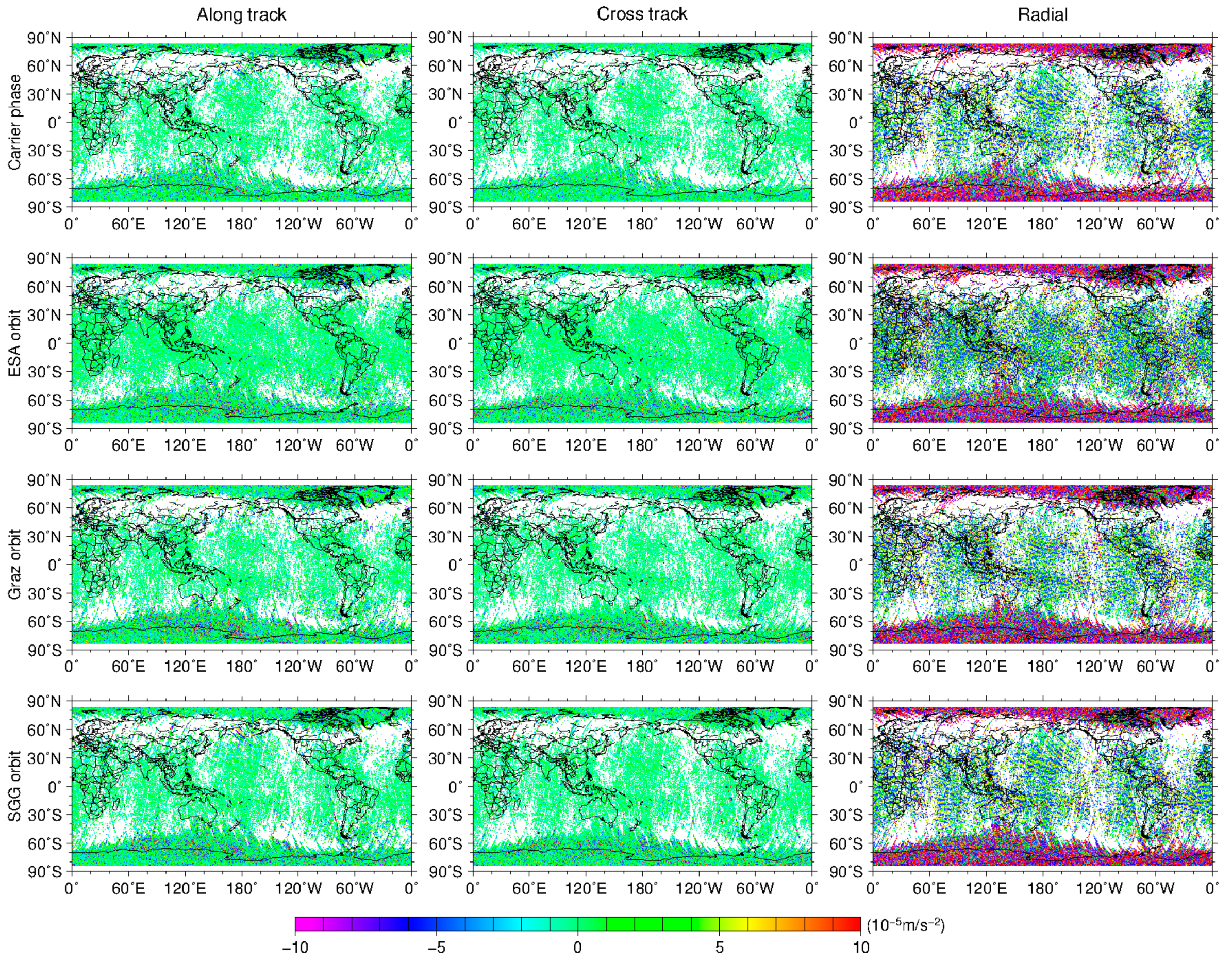
4. Discussion

According to Figure 1 and Figure 2 as well as Table 4, the derived radial accelerations were noisier than the other two components. This can be explained by a relatively low accuracy of the GPS positioning in the radial direction, which is caused by the geometric configuration of the satellite constellation [44,45,46]. Additionally, the along-track accelerations performed weaker than the cross-track component, which was caused by an increase or decrease in the number of visible satellites because geometry changes can inevitably degrade the position solution and create large acceleration errors [46]. Therefore, stringent position accuracies and poor tolerance of geometry changes are the main drawbacks of the orbit differentiation method. However, the carrier phase differentiation method is more robust because no ambiguity resolution is required. 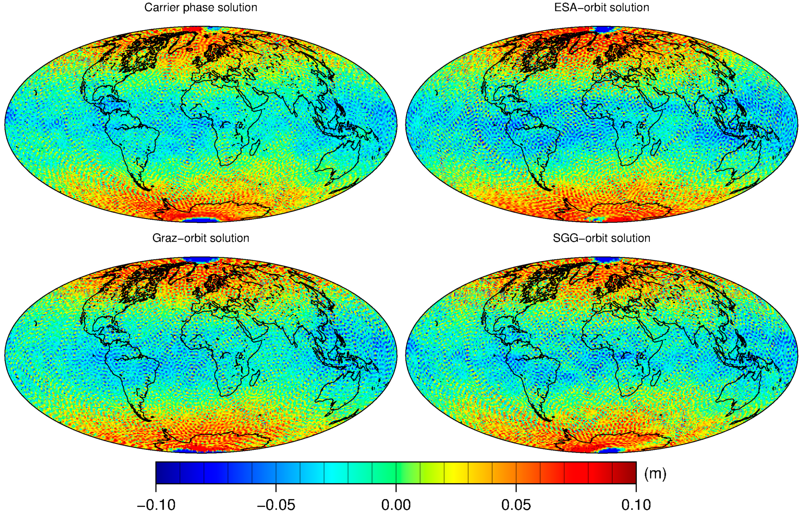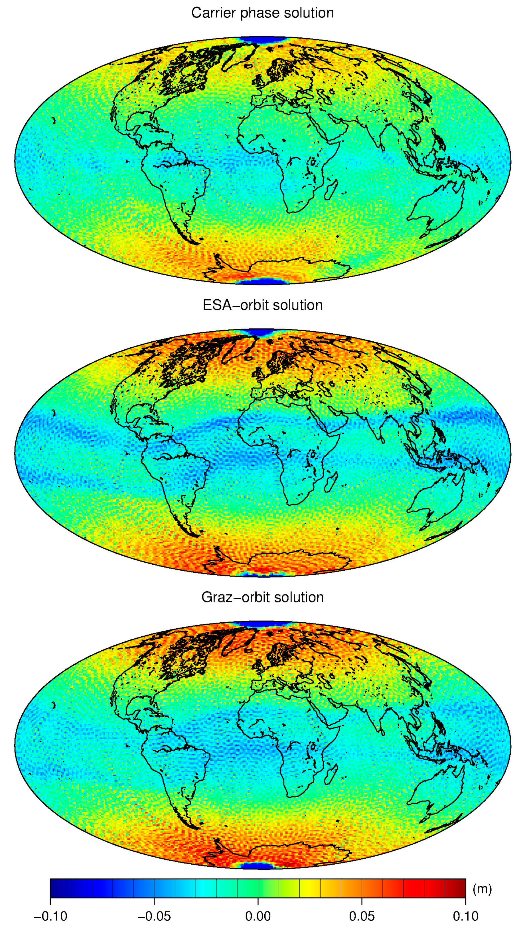In addition, the distribution of gross errors in Figure 1 and geoidal errors in Figure 5 and Figure 7 were geographically correlated and highly inhomogeneous; large errors were mainly located close to the geomagnetic poles. There are two reasons for this situation: the poor observation geometry in geographical polar region, which is very close to the geomagnetic polar region; and the ionospheric scintillation effects, which cause short-period irregular changes in the phase and amplitude of signal [44].

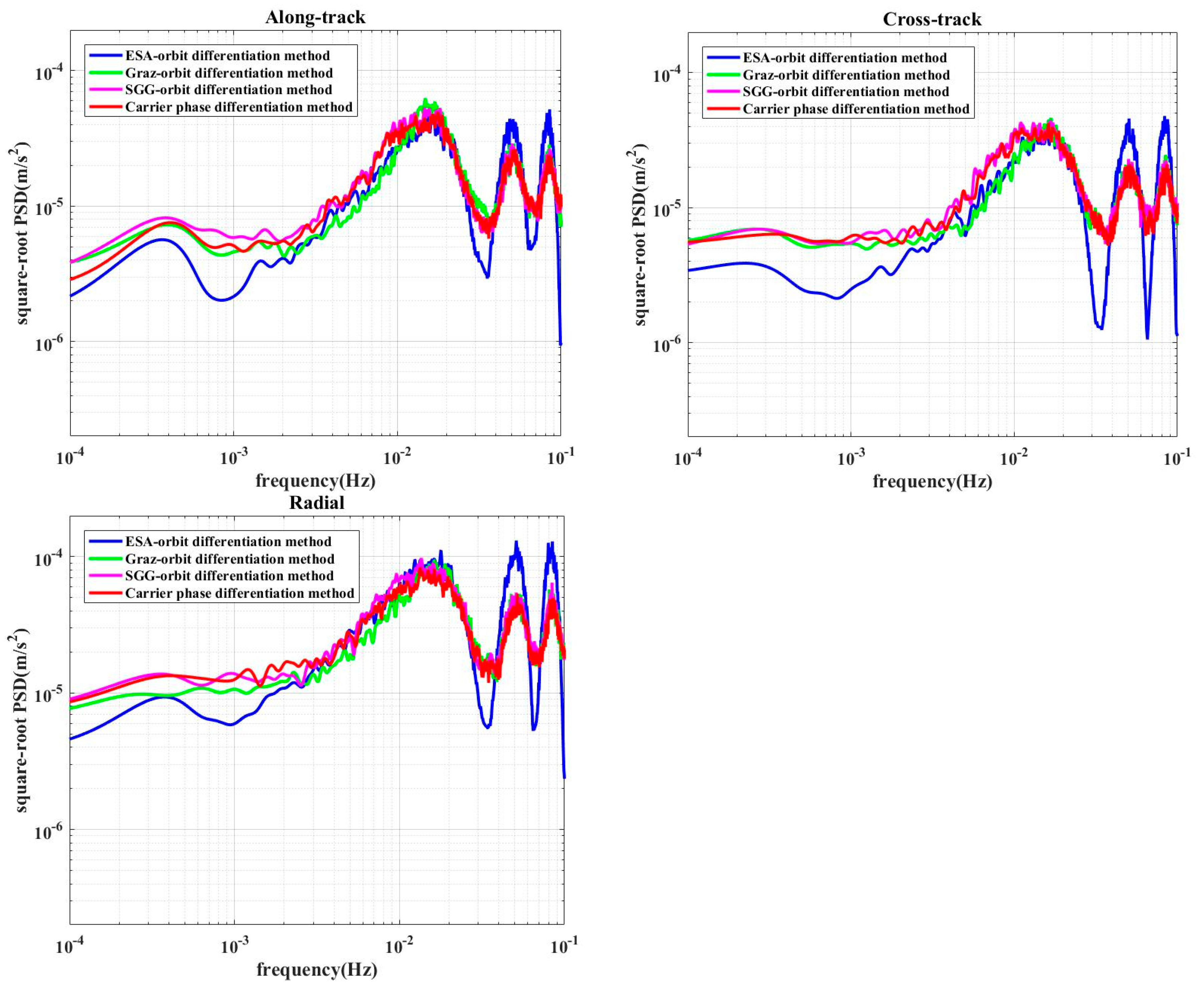
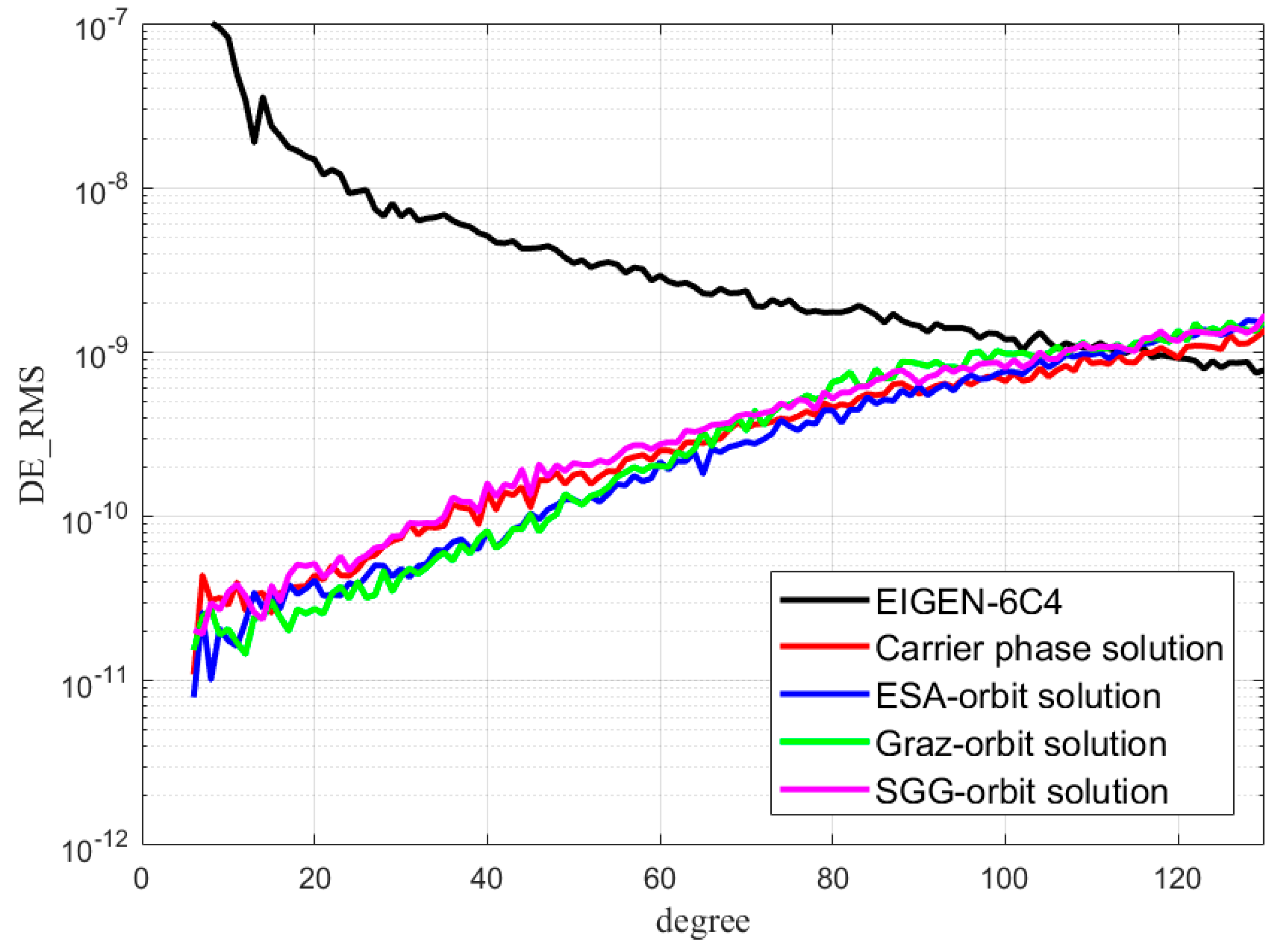
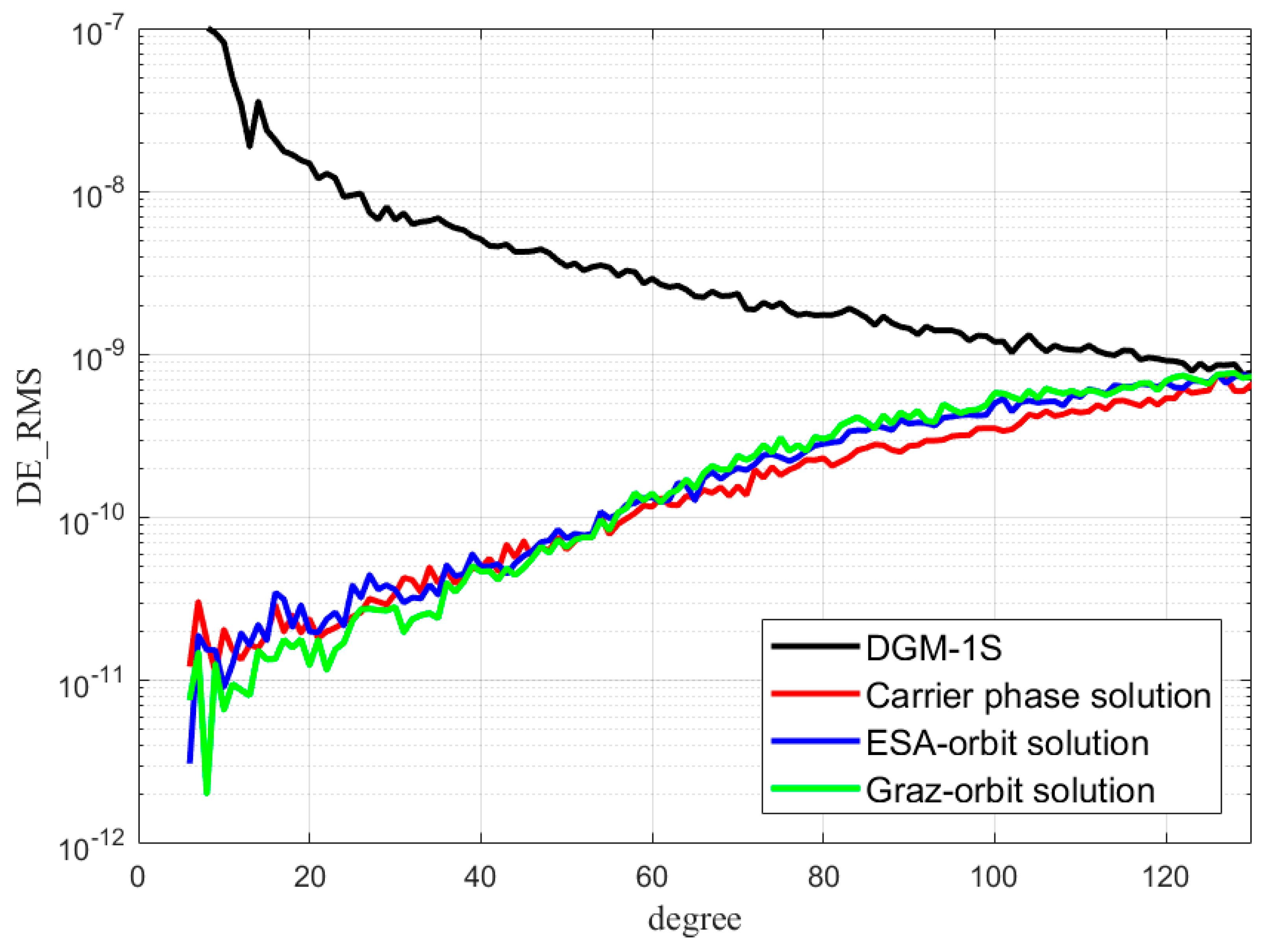
According to Figure 4 and Figure 6 as well as Table 5 and Table 7, the carrier phase solution showed a slightly better performance than the other solutions derived from the orbits only in the high-frequency portion; the 71-day solution corresponds to degree n > 100 and 2.5-year solution corresponds to degree n > 70. In this frequency band, the acceleration noise of the carrier phase solution was lower than the others, as shown in Figure 2. The degrees 100 and 70 approximately correspond to the frequency 0.019 and 0.013 Hz. In comparison with the Graz-orbit solution, the carrier phase solution had a lower accuracy for the degree n < 70 and a higher accuracy for n > 70, which is consistent with frequencies less than 0.013 Hz (approximately corresponding to the degree 70). Moreover, the cumulative geoid height differences of the Graz-orbit, ESA-orbit, and carrier phase solutions up to degree 50 were 0.97, 1.01, and 1.08 cm, respectively, as seen in in Table 7, which shows that the Graz-orbit solution had the highest precision for the degrees lower than 50. In Table 5, the carrier phase solution was better than the SGG-orbit solution for almost all degrees (n > 30), and the accuracy improvement of geoid height up to d/o 130 was 21%, which is similar to that in Guo et al. [25]. A comparison of Figure 4 and Figure 6 as well as Table 5 and Table 7 indicates that the longer data period has improved the solutions significantly along the entire frequency band. In addition, as depicted in Figure 5 and Figure 7, the pronounced errors along the geomagnetic equator were observed in all solutions. This is a result of the high electron density in addition to large short-term variations in the ionosphere near the geomagnetic equator [47,48].

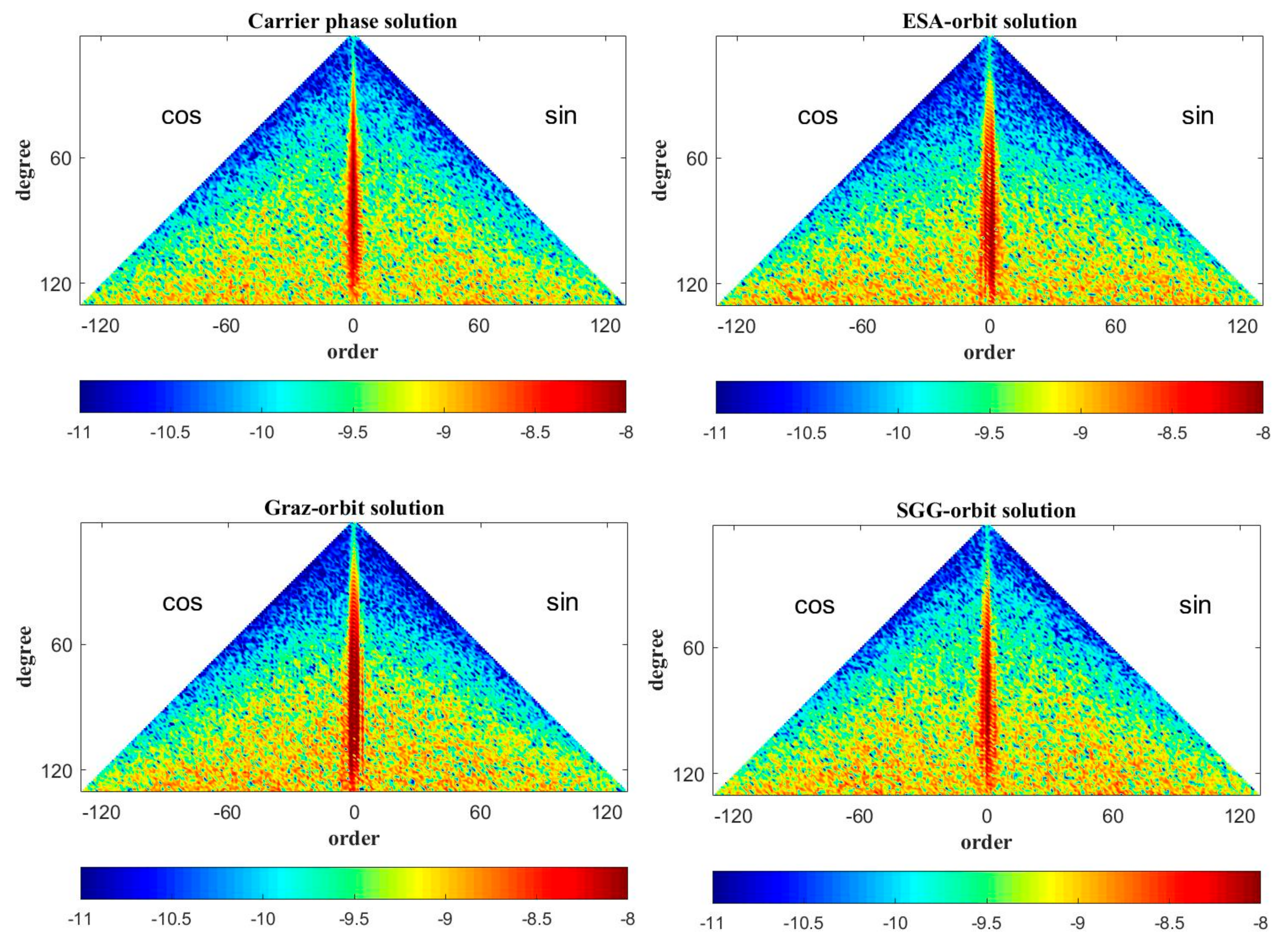
As shown in Figure 3, the zonal and near-zonal spherical harmonics coefficients of the recovered models were worse than the other coefficients due to the fact that the GOCE satellite flies in a sun synchronous orbit with an inclination of 96.7°, which causes the ill-posed problem of the least squares used for recovering the gravity field model [49,50]. However, zonal harmonic coefficients estimated by the carrier phase differentiation method were slightly better than those from the orbit differentiation method.

5. Conclusions

The point-wise acceleration approach was proposed to recover the gravity field model based on satellite accelerations directly estimated from the GOCE’s onboard carrier phase observations. The satellite accelerations derived by the carrier phase differentiation method had a slightly better quality in terms of time-domain than those derived by the kinematic orbit differentiation method, respectively. A static gravity field model up to degree and order 130 was compiled from 71 days and 2.5 years of GOCE SST-hl data by the carrier phase differentiation method. Additionally, the gravity models were estimated based on the conventional orbit differentiation method from the ESA’s, Graz’s, and SGG’s PKI orbits. In comparison with the reference models (EIGEN-6C4 and DGM-1S) in accordance with DE-RMS, the 71-day carrier phase solution was slightly better than the SGG-orbit solution in the entire frequency band; however, it showed a worse performance in the low frequency part than the ESA-orbit solution and Graz-orbit solution. Furthermore, the 2.5-year carrier phase solution had the best accuracy for the degrees greater than 70, and its cumulative geoid height error up to d/o 130 was the lowest, which indicates that the proposed approach in this paper shows very good performance for gravity field modeling from the SST-hl observations.

The empirical variance-covariance matrices used in this paper were constructed directly by using the residual accelerations. In the future, the variance-covariance matrix can be derived by using the error propagation method from the prior carrier phase and orbital variance-covariance information.