Article

End-to-End Instrument Performance Simulation System (EIPS) Framework: Application to Satellite Microwave Atmospheric Sounding Systems

1
Astronomy Instrumentation Group (AIG), School of Physics and Astronomy, Cardiff University, Queen’s Buildings, The Parade, Cardiff CF24 3AA, Wales, UK
2
Met Office, FitzRoy Road, Exeter, Devon EX1 3PB, UK
3
Quantum Sensors Group, Cavendish Laboratory, University of Cambridge, JJ Thomson Avenue, Cambridge CB3 0HE, UK
*
Author to whom correspondence should be addressed.
Remote Sens. 2019, 11(12), 1412; https://doi.org/10.3390/rs11121412
Submission received: 23 April 2019 / Revised: 31 May 2019 / Accepted: 12 June 2019 / Published: 14 June 2019
(This article belongs to the Section Atmospheric Remote Sensing)

Abstract

:
This article presents a generic flexible framework for an End-to-end Instrument Performance Simulation System (EIPS) for satellite atmospheric remote sensing instruments. A systematic process for developing an end-to-end simulation system based on Rodgers’ atmospheric observing system design process has been visualised. The EIPS has been developed to support the quantitative evaluation of new satellite instrument concepts in terms of performance simulations, design optimisation, and trade-off analysis. Important features of this framework include: fast radiative transfer simulation capabilities (fast computation and line-by-line like simulations), applicability across the whole electromagnetic (EM) spectrum and a number of integrated retrieval diagnostics. Because of its applicability across the whole EM spectrum, the framework can be usefully applied to synergistic atmospheric retrieval studies. The framework is continually developing and evolving, and finding applications to support and evaluate emerging instrument and mission concepts. To demonstrate the framework’s flexibility in relation to advanced sensor technologies in the microwave range, a novel superconducting transition edge sensor (TES) -based multi-spectral microwave instrument has been presented as an example. As a case study, the performance of existing multi-spectral-type microwave instruments and a TES-technology-based multi-spectral microwave instrument has been simulated and compared using the developed end-to-end simulation framework.

Graphical Abstract

1. Introduction

Satellite remote sensing instruments operating in the infrared (IR) and microwave (MW) regions of the electromagnetic (EM) spectrum provide key information for global numerical weather prediction (NWP) models. Currently, more than 90% of all observational data assimilated in global NWP systems comes from satellites. When considering satellite observations only, the MW and IR sounders together make up about 79% of the positive impact of all satellite observations; 45% is from MW soundings and the other 34% from IR soundings [1,2]. Major contributors to the reduction of forecast errors from temperature soundings are the Advanced Microwave Sounding Unit-A (AMSU-A - on board several platforms) and the Infrared Atmospheric Sounding Interferometer (IASI) hyperspectral instrument on board Meteorological Operational (MetOp) satellites [3,4,5,6,7,8,9]. For water vapour retrieval, currently one of the most informative satellite radiometers for humidity soundings is the Advanced Microwave Sounding Unit-B/Microwave Humidity Sounder (AMSU-B/MHS). The remote sensing data from these IR and MW instruments are useful for the retrieval of atmospheric temperature and water vapour vertical profiles [10,11] and other atmospheric parameters.
However, all of these instruments have drawbacks. Retrievals from IR hyperspectral instruments such as the IASI are considered to be of high quality. But these observations are restricted to clear sky conditions. The MW instruments can see down into clouds, and therefore provide important information about the atmospheric state and hydrometeors (rain, ice etc.), and they are also used for the retrieval of sea surface parameters (e.g. sea surface temperature [12]). But the vertical resolution is very poor, due to the very limited number of sounding channels. The radiometric noise in these channels is also a limitation on performance. In future, it can be expected that there will be an increase in the number of satellite microwave sounding instruments, covering a wide range of applications including NWP (MicroWave Sounder (MWS) [13], MicroWave Imager (MWI) [13,14]), climatology (Ice Cloud Imager (ICI) [13,14]), precipitation monitoring and severe weather events (Geostationary Observatory for Microwave Atmospheric Sounding (GOMAS) [15]). Furthermore, recent technological advancements in MW sensors and instrumentation has paved the way for the development of new and advanced satellite MW remote sensing instrument concepts.
An example of one such technology advancement is the development of on-chip superconducting filterbank spectrometers. This state-of-the-art technology will enable hundreds of spectral channels in the MW region, with individually tailored bandwidths, and resolution (ν/Δν) greater than ~1000, sensed down to the photon-noise limit [16]. Superconducting filterbank spectrometers differ from “conventional” heterodyne-based solutions in three main ways. Firstly, there is no down conversion stage; both the filters and power detectors operate at the signal frequency. Secondly, both the filterbank and detectors are implemented using superconducting technologies. Thirdly and importantly, the filterbanks and detectors are integrated together on the same device chip. The basic concept is illustrated in Figure 1.
The signal from the observed scene is coupled via a broadband antenna to a mm-wave microstrip feed line. Half-wave resonator filters are capacitively coupled to the microstrip feed line and to a transition edge superconducting (TES) detector. The spectral characteristics of each filter are determined by the resonant behaviour of filter line section and by the strength of coupling to the feed and detector. The superconducting filterbank approach delivers a large number of narrow and very low noise spectral channels in a small and rugged package. The design of the filters gives great control over channel placement and shape, and these need not be regular. This combination is near ideal for a hyperspectral sounding instrument: close-packed arrays of narrow channels can be provided to cover key lines in a wide bandwidth, along with broad channels for background subtraction.
Technology advancements naturally lead to promising new instrument concepts for applications in different types of atmospheric monitoring areas, above and beyond temperature and humidity sounding and cloud sensing, etc. The development and definition of instrument concepts requires consideration of many interlinked design factors, such as observational requirements (geophysical variables to be measured), technology requirements and limitations, mission requirements etc. Trade-off analysis between these parameters is necessary to identify the instrument design that provides the optimum performance [17]. To quantitatively analyse the performance of an instrument and to optimise its concept design via trade-off analysis, the implementation of an end-to-end simulation process is required. An end-to-end simulation is an important part of the atmospheric observing system design process [18]. To support studies related to new instrument concepts and their evaluation for atmospheric remote sensing and NWP applications, we have developed a generic end-to-end instrument performance simulation system (EIPS) framework for satellite atmospheric sounding instruments. The radiative transfer forward model which is incorporated as one of the component of EIPS framework is the Havemann-Taylor Fast Radiative Transfer Code (HT-FRTC) [19]. The HT-FRTC has been applied across the EM spectrum in a number of previous studies, both in the infrared [20,21,22,23] and in the short-wave and part of the ultraviolet [24,25]. The HT-FRTC has been used to evaluate different configurations of an infrared satellite radiometer concept based on laser heterodyne technology [26]. Using the HT-FRTC, the EIPS framework becomes applicable to any passive spectral sensor from the ultraviolet (UV) to the microwave (MW). This paper is focused on the application of EIPS framework to satellite sensors in the MW spectral range.
The purpose of this paper is to give an overview of the EIPS framework and to describe the framework design, the component models and their organisation. To demonstrate the framework’s flexibility in relation to advanced sensor technologies in the MW, a novel superconducting transition edge sensor (TES) based multi-spectral MW instrument has been presented as an example. Furthermore, as an example of the framework’s application, we have applied it by conducting a case study, in which we analysed and compared the relative performance of existing multi-spectral type MW instruments with a TES technology based multi-spectral MW instrument.
In Section 2 of this paper, we present a useful overview and a visualisation of a general atmospheric observing system design process using which the EIPS framework has been derived. The description of the EIPS framework, its building blocks, and their organisation are presented in Section 3. And in Section 4 we present the application of EIPS framework through a case study of comparative performance analysis between existing and emerging technology-based satellite MW remote sensing instruments (as described in above paragraph).

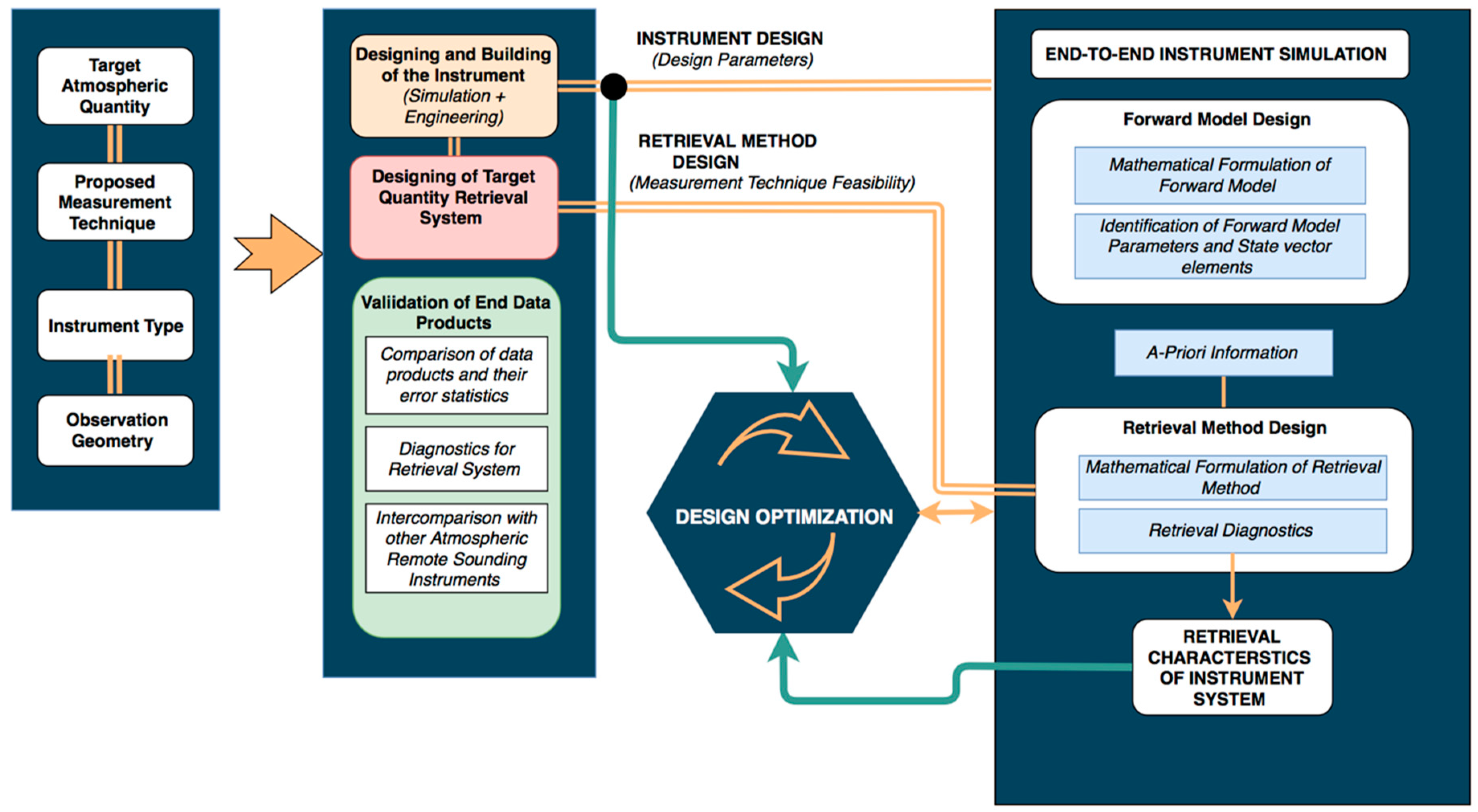
2. Satellite Atmospheric Observing System Design

We developed our end-to-end simulation framework for designing an atmospheric observing system, using a systematic approach given in Rodgers [18]. We first present a simple visualisation of this atmospheric observing system design (AOSD) process in the form of a schematic block diagram in Figure 2; then, we use this as a guideline to build our EIPS framework. It is very important that any end-to-end simulation system should encompass all the physical processes and factors related to the design of a satellite instrument.
A generic end-to-end atmospheric remote sensing simulation system should comprise at least three main components:
  • Sensor modelling: this should take account of all the instrument system parameters that can affect the measurement of the signal such as: spectral response function (SRF), detector noise etc.,
  • Atmospheric radiative transfer modelling: modelling of the propagation of EM radiation through the earth’s atmosphere,
  • Inversion algorithm: an algorithm is required to retrieve the geophysical variables of interest and to test their accuracy and sensitivity to other factors.

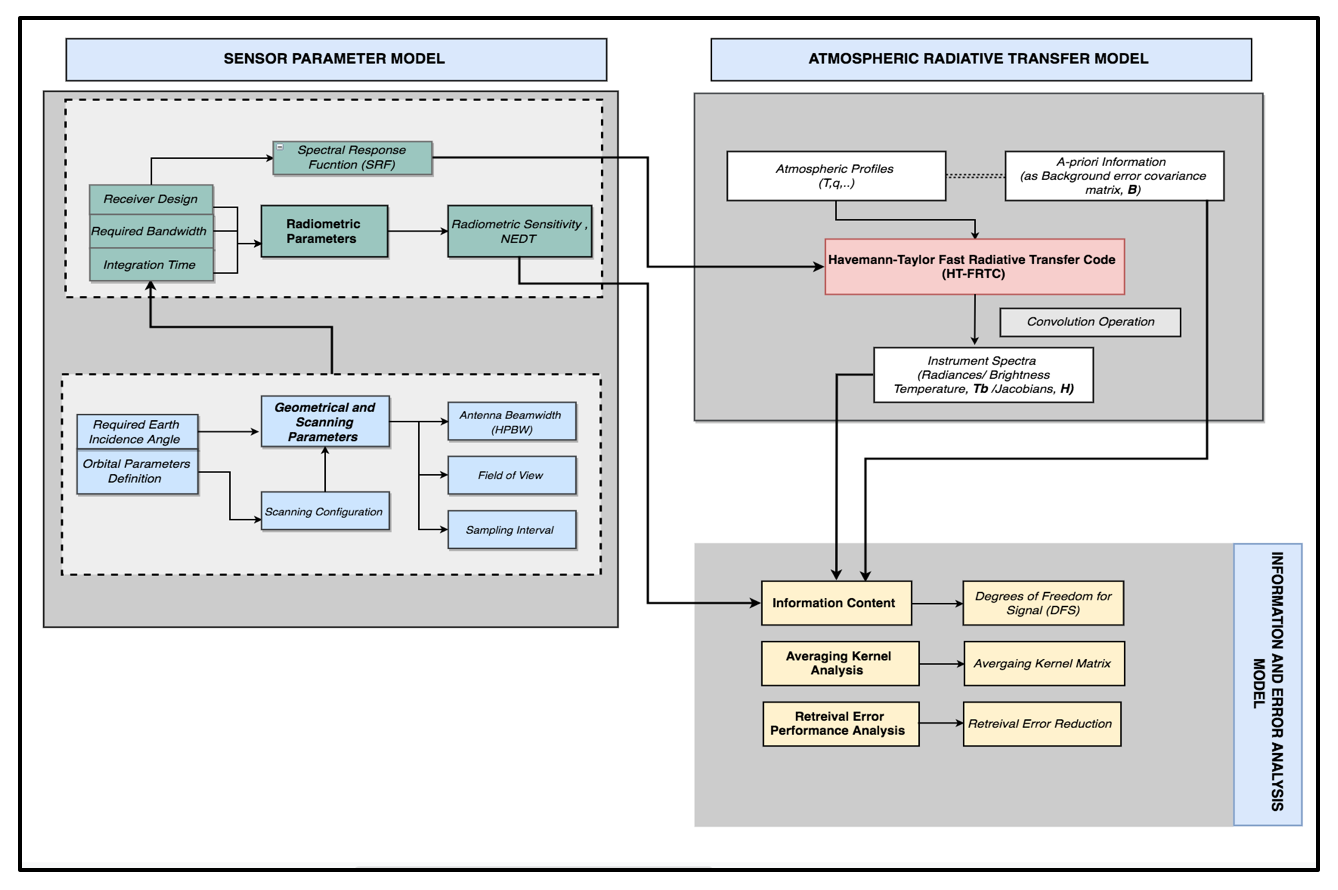
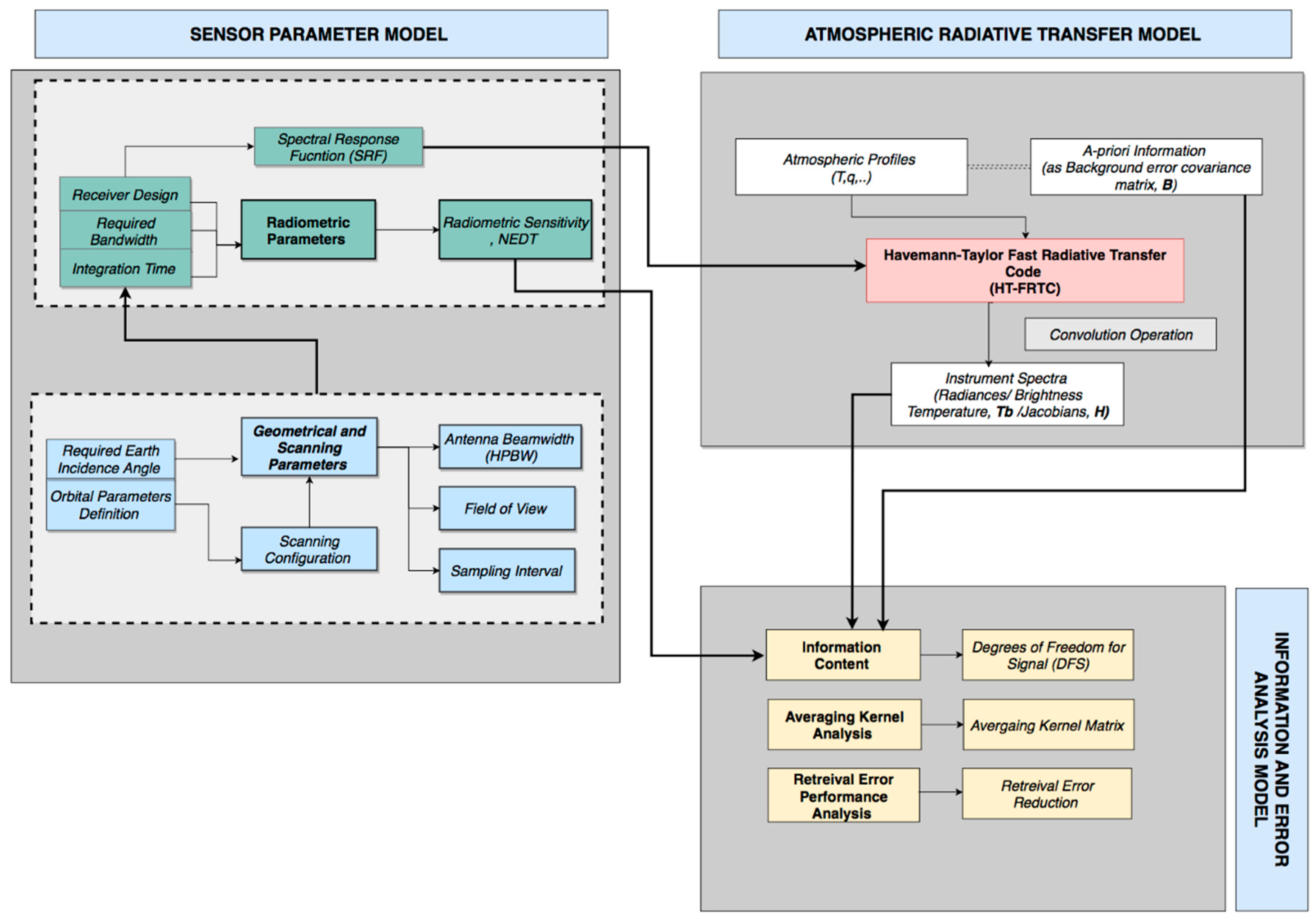
3. The End-to-End Instrument Performance Simulation System (EIPS) Framework

The EIPS framework has been designed following the process discussed in Section 2 (as shown in Figure 2). It incorporates a sensor model, an atmospheric radiative transfer model and an inversion algorithm. To make the framework applicable to whole EM spectrum, we decided to incorporate a state-of-the-art radiative transfer model, the Havemann-Taylor Fast Radiative Transfer Code (HT-FRTC) [19] for fast radiative transfer simulation capabilities (see Section 3.2.2 for details). The basic aim behind EIPS was to design a framework around the HT-FRTC model to obtain a complete and flexible end-to-end simulation tool for instrument performance analysis purposes. For sensor related computational simulations, a sensor parameter model has been developed (see Section 3.2.1), and for atmospheric retrievals, an information and error analysis model has been developed (see Section 3.2.4).
In this way, the EIPS will provide combined functionality of sensor parameter modelling, fast radiative transfer simulation (by the HT-FRTC), and geophysical parameter retrievals. Since the HT-FRTC is applicable to whole EM spectrum, the EIPS can be applied to any remote sensing instrument operating in any spectral range (UV, IR and MW) with appropriate tuning in the component models.

3.1. EIPS Block Design and Organisation

Here we discuss the component models of the EIPS. In the top-level, the EIPS framework can be decomposed into: (1) the sensor parameter model, (2) the atmospheric radiative transfer model, and (3) the information and error analysis model. These component models will provide the three main elements of our end-to-end simulation system (as discussed in Section 2). The organisation of these component models to form the EIPS framework is represented with the help of a schematic block diagram in Figure 3.

3.2. EIPS Components

3.2.1. Sensor Parameter Model

A sensor parameter model has been developed for modelling of sensor characteristics. The sensor model simulates the instrument and mission profile, taking into account key instrument design factors such as observation geometry, scan strategy, detector type, instrument configuration, channel characteristics, and calculates the radiometric sensitivity of the instrument in terms of noise equivalent temperature difference (NETD) per spectral band and the SRF (and the SRF files essentially contains the list of sounding spectral channels, with their associated bandwidths). Here, we define NETD as the temperature difference that would produce a detected signal-to-noise ratio of 1 in a 0.5 second integration time, or a post-detection bandwidth of 1Hz.

3.2.2. Atmospheric Radiative Transfer Model: The HT-FRTC

The theoretical background and development of the HT-FRTC is given in detail in [19]; here, we will give a brief description of important functionalities of HT-FRTC in the context of development of our EIPS framework. The HT-FRTC is a principal component (PC) based model and can be used for calculating transmittance(s), radiance(s) and Jacobian(s) across the EM spectrum from UV to MW represented by their principal components [19]. The code can be run for any user-defined vertical atmospheric pressure grid [19]. Absorption properties of atmospheric trace gases and it’s treatment in the HT-FRTC is given and explained in [19].
The simulations using the HT-FRTC model can be performed in two modes: line-by-line and fast. But in the EIPS, only the fast mode of the HT-FRTC has been incorporated, with which many thousands of atmospheric profiles can be easily processed and a full line-by-line like resolution output can be produced. The HT-FRTC is, to our knowledge, unique in allowing fast simulations at a full line-by-line resolution which are sensor independent and therefore simplify studies of different instrument configurations. Thousands of profiles can be easily processed. In a future operational NWP data assimilation systems, setting a fast code will have to be used in order to be able to process the expected large data volumes in a timely manner. The accuracy of the fast code has been evaluated by comparing its results with line-by-line code results for the profiles used in this study. These profiles are independent from the profiles used for the training of the fast code, which are sampled from a database of ECMWF atmospheric profiles as explained in more detail in [19]. As can be seen in Figure 4a, the fast code is nearly unbiased against the line code with maximum biases of around 1 millikelvin. The standard deviation between the two codes is larger, but does not exceed 20 millikelvin (see Figure 4b). We consider this level of accuracy to be acceptable for the purposes of the studies within the EIPS framework. The accuracy of the line-by-line code will itself be limited in turn by the uncertainties in the knowledge of the spectroscopy, which is difficult to quantify and beyond the scope of this paper.

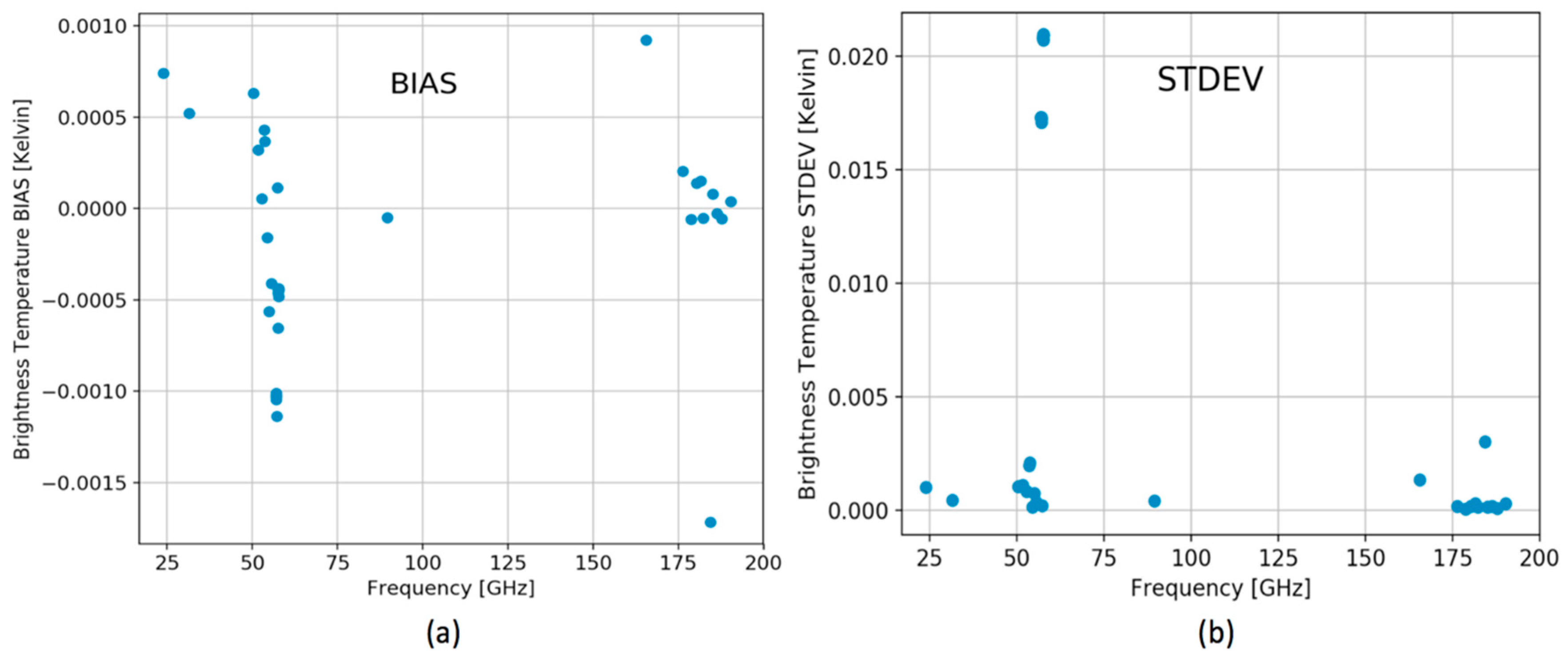
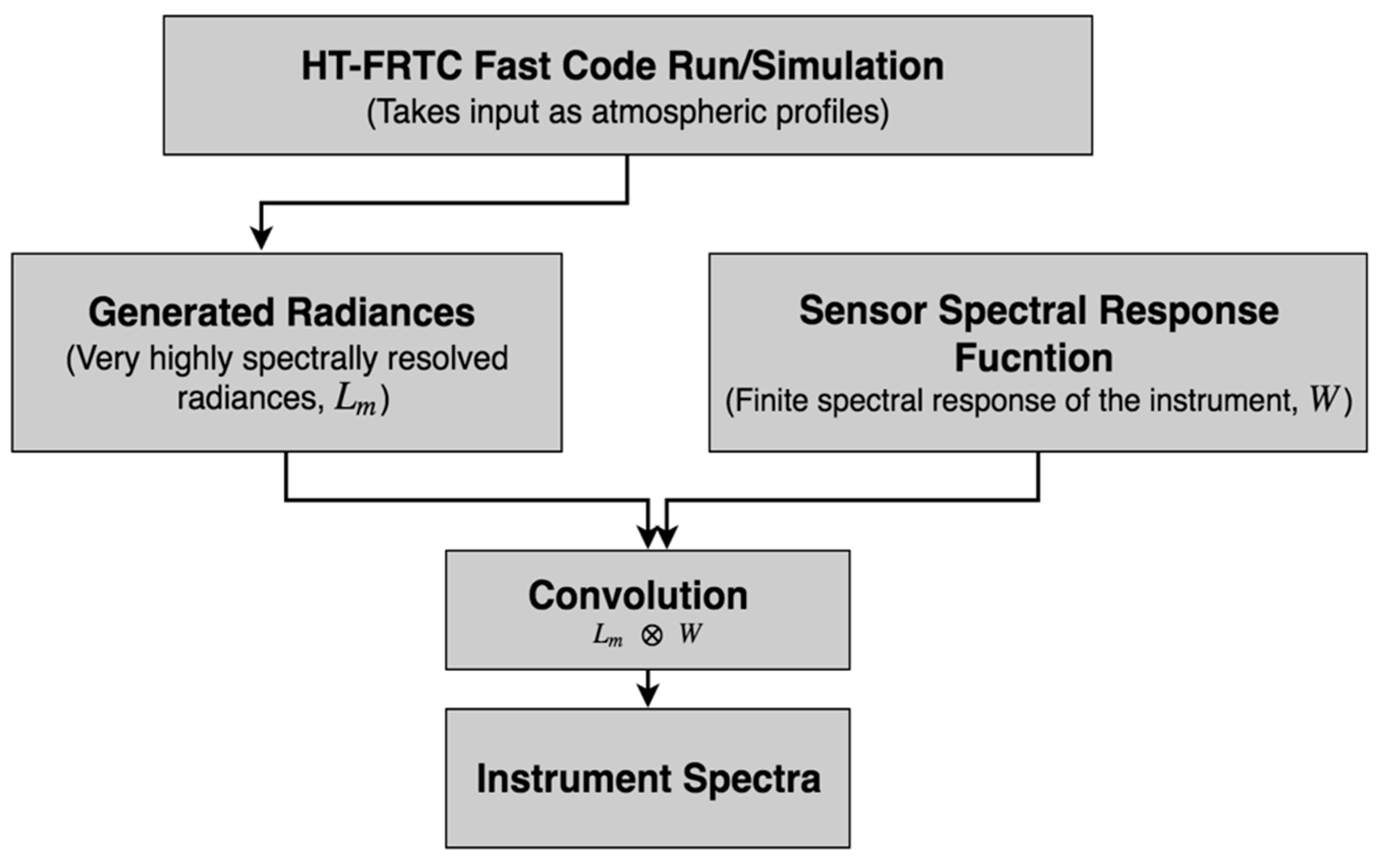
3.2.3. Sensor Component of the HT-FRTC

The advantage of using a fast mode of the HT-FRTC within the EIPS framework is that it does not require instrument-specific coefficients, in comparison to conventional fast radiative transfer models like the Radiative Transfer for TOVS (RTTOV; TOVS stands for TIROS Operational Vertical Sounder and TIROS for Television InfraRed Observation Satellite) [27]. The fast mode uses a small number of about 300 monochromatic frequencies as predictors for the PC scores. The PCs themselves are derived during the training at a very high spectral resolution (HT-FRTC calculations were done at a spectral resolution of 3 MHz) and are independent of any instrument parameters. Simulated spectra for any particular instrument can be constructed by the convolution with the sensor SRF either on the level of radiances or on the level of PCs. Convolution of highly spectrally radiances with instrument specific SRFs offers the flexibility of taking any type of instrument line shape only at the last step of the process. This process of construction of instrument simulated spectra using convolution of highly spectrally resolved radiances with sensor SRFs is represented in the flow diagram in Figure 5. This specific property of HT-FRTC makes it very useful for studies related to new instruments and for investigating large number of instrument configurations.

3.2.4. Information and Error Analysis Model

An important objective of an end-to-end simulation is to quantify the performance of the instrument and to optimise the instrument parameters with respect to retrieval parameters [18]. To obtain that functionality, an information and error analysis model has been developed (in the EIPS framework) based on the principles of optimal estimation (OE) [18].

3.2.4.1. Theory of Optimal Estimation

This section briefly describes the theory of OE applied in context of atmospheric sounding for developing the information and error analysis model. There are at least two notations used, but we adopt the standard data assimilation notation of [28] to briefly to explain the OE theory. We start with the mathematical notations for the forward model, which is a radiative transfer model in the context of atmospheric sounding.
A forward model (F) can be mathematically written as:
y = F ( x ) + ϵ
where y is the measured signal spectrum, x is the true state of the atmosphere to be estimated and ϵ is the error in the measurements. Solutions to the Equation (1) can be estimated in the maximum a-posteriori (MAP) framework, from which the equation for the retrieved atmospheric state ( x ^ ) can be derived as:
x ^ = x a + ( H T R 1 H + B 1 ) 1 H T R 1 ( y F ( x a ) )
x ^ = x a + G ( y F ( x a ) )
where H is the Jacobian matrix, R is the observation error covariance matrix, and G is the gain matrix and A is the analysis error covariance matrix. With proper specification of an a priori error covariance matrix B (which often comes from the short numerical range forecast), the retrieval errors can be estimated by the A matrix which is given by the following Equation (4):
A = ( B 1 + H T R 1 H ) 1
This analysis error covariance matrix is very useful for estimating the retrieval error without exactly calculating the retrievals and for comparing the retrieval error performance of different instrument configurations.

3.2.4.2. Retrievals and performance diagnostics

For testing and analysing the performance of an atmospheric remote sensing instrument, the information and error analysis model has been integrated with various useful OE-based retrieval diagnostics:
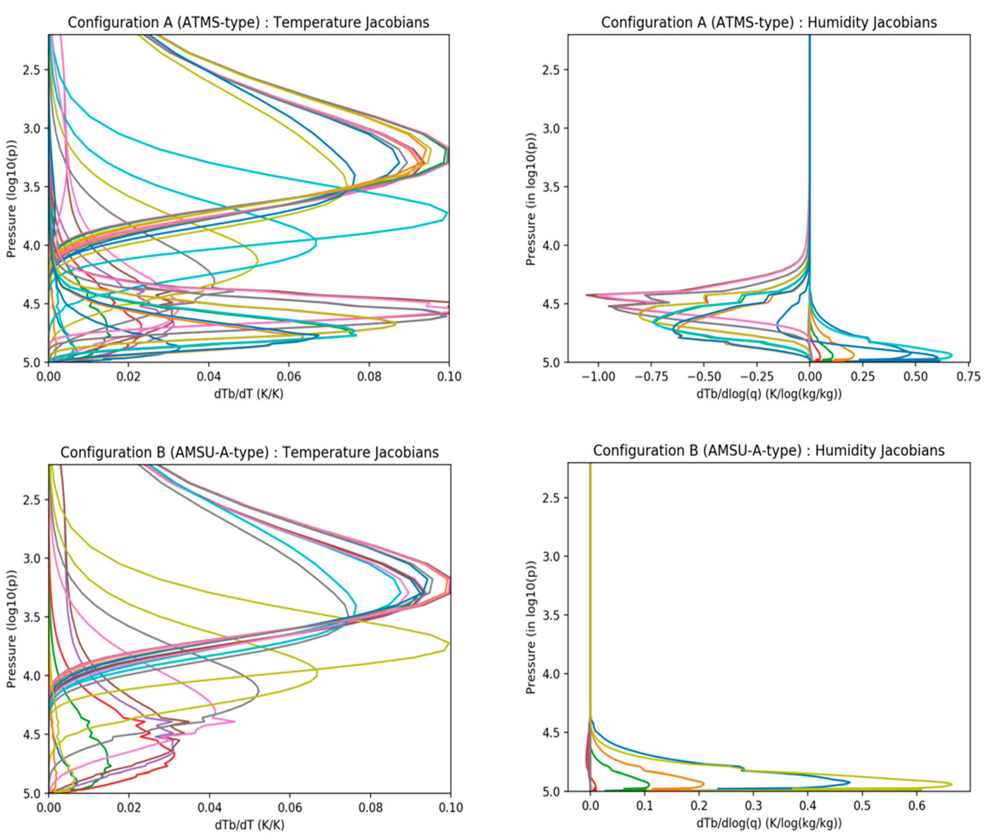
  • Jacobian Matrix: The elements of the Jacobian matrix provides the sensitivity of the satellite measurements with respect to the target atmospheric parameters. These Jacobians play an important role in the spectral channels design and placement in the EM spectrum. The mathematical expression for the Jacobian matrix is given by the following Equation (5):
    H = y x
  • Retrieval Errors: Retrieval errors are given by the square root of diagonal elements of analysis error covariance matrix A . Comparison of analysis errors with the background errors gives the reduction in the retrieval error, and which is also a measure of retrieval error performance of an instrument. Retrieval and background errors can be calculated by the mathematical expressions (6) and (7) respectively:
    a ii = diag ( A )
    b ii = diag ( B )
    where a ii and b ii are the elements on the ith row and ith column of A and B matrix respectively and diag ( . ) denotes the leading diagonal of the matrix.
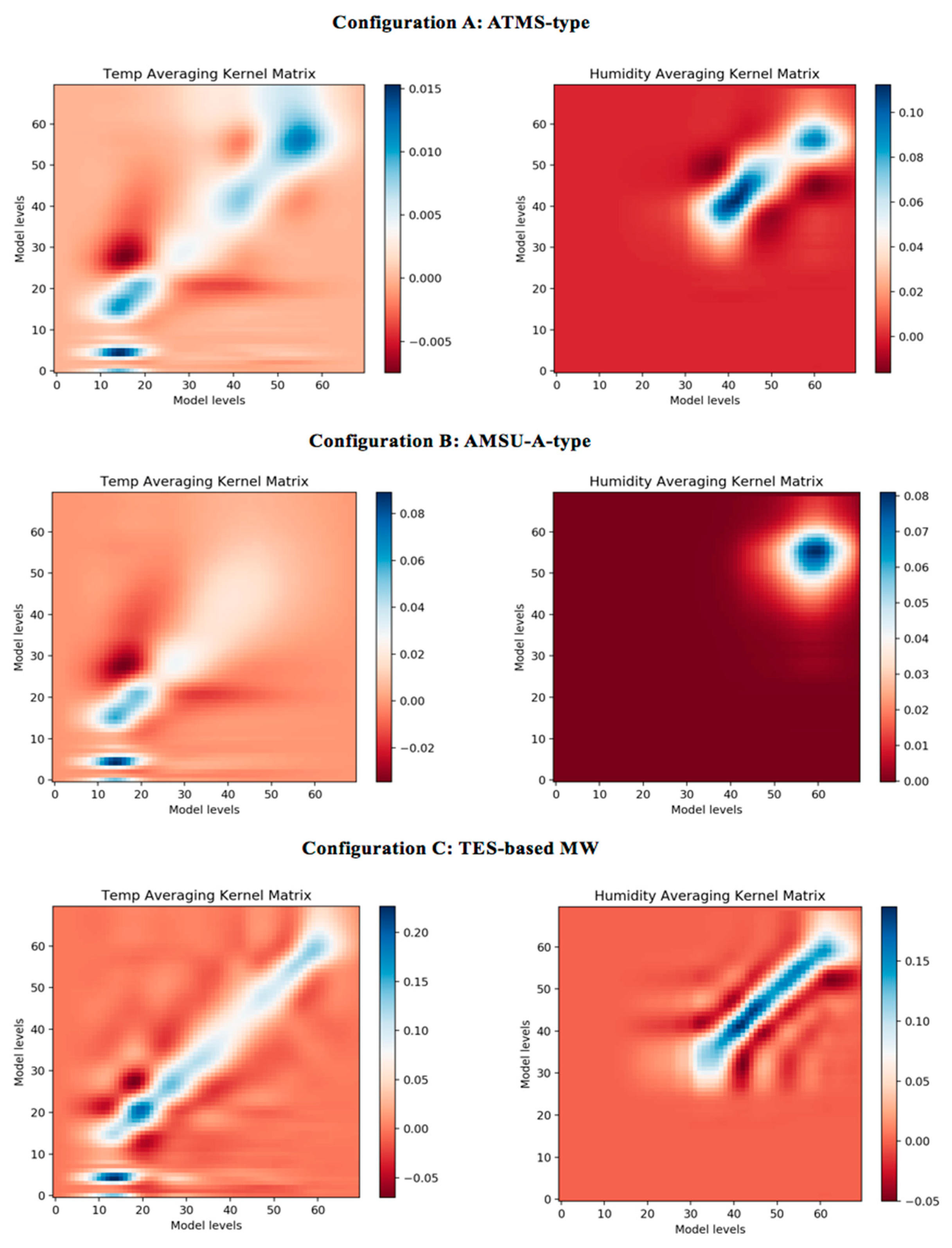
  • Averaging Kernels: Averaging kernels are defined as the sensitivity of the retrieval state with respect to the true state of the atmosphere. Mathematically, these averaging kernels can be formulated as:
    U = x ^ x = ( H T R 1 H + B 1 ) 1 H T R 1 H
    where U is the averaging kernel matrix, x ^ is the retrieved atmospheric parameter and x is true state of the atmospheric parameter.
  • Degrees of Freedom for Signal (DFS): Information content is another important diagnostic for measuring the performance of an atmospheric observing system. Information content of satellite measurements can be estimated by comparing retrieval error covariance matrix A with the background error covariance matrix B . In the context of EIPS framework, the Degrees of Freedom for Signal (DFS) has been incorporated as the measure of information content, and it is given by the Equation (9):
    d s = tr ( I A B 1 )
    where d s is the degrees of freedom for signal, and tr (.) denotes the trace of a matrix.

4. Example of Application: Performance Simulations using the EIPS framework

In this section, our aim is to apply the EIPS framework for performance simulations by conducting a study of analysis of relative information content of current and emerging multi-spectral MW remote sensing systems for temperature and humidity sounding applications.

4.1. End-to-End Simualtion Settings and Inputs

We first start by setting up three hypothetical MW instrument configurations namely A, B and C. Configuration A and B are based on existing multi-spectral MW instrument technology and C is based on recently developed technology (see Section 4.2.2). Some of the parameters for all the three instrument configurations have been taken as common to avoid any complexity in comparing the simulated results in context of this paper. These common parameters were set up in the EIPS, and are shown in the Table 1. EIPS component models require different inputs to start the end-to-end simulation process such as: atmospheric profiles (as an input to the HT-FRTC model) and a background error covariance matrix (as an input to the information and error analysis model).
For input to the HT-FRTC model, a set of eight atmospheric profiles have been taken for calculating Jacobians. These atmospheric profiles are on the 70 Met Office Unified Model (UM) levels and spanning range of latitudes and atmospheric conditions. Out of the eight profiles, profile 1 is the US standard atmosphere and seven of these profiles (Profile 2 to 8) have been extracted directly from the Met Office UM in March 2012. These profiles have been used in recent studies in [26,29]. The background error-covariance matrix was constructed using a randomisation method. The matrix is a 1D representation of the temperature-based component of the 4D-Var error covariance which was in operational use at the Met Office in March 2012. The B matrix used here was described in detail and used in experimental simulations in [26] and in [30].

4.2. Microwave System Configurations

4.2.1. Configuration A: ATMS-Type and Configuration B: AMSU-A-Type

Configuration A corresponds to an existing MW instrument, the Advanced Technology Microwave Sounder (ATMS) (“ATMS-type”) and configuration B corresponds to Advanced Microwave Sounding Unit-A (“AMSU-A-type”). The spectral and radiometric characteristics of configuration A and B has been kept exactly the same as the ATMS and AMSU-A instruments respectively (see Table 2).

4.2.2. Configuration C: TES-Based MW Instrument

Superconducting transition edge sensor (TES)-based filterbank spectrometer technology has recently been developed for enabling a future ultra-low-noise hyperspectral MW instrument for atmospheric remote sensing applications [16]. For the purposes of this illustration only, we simulate a proposed multi-spectral instrument based on this superconducting filterbank technology, but with a channel configuration that exactly replicates those of ATMS. In this way, we can directly compare the impact of instrument noise on the information content for each instrument. The channel characteristics of configuration C (a TES technology-based MW Sounder) have been kept same as those in configuration A. The sensor parameter model for this new technology-based instrument has been used to estimate the radiometric sensitivities, as shown in Table 2.

4.3. Performance Simulations Analysis Using EIPS Framework

After fixing all the inputs and settings (as described in Section 4.1 and in Table 1) needed for performance simulations, we run the EIPS framework for all three MW system configurations in an end-to-end manner. The output of these simulations is then used to analyse the performance of these instrument configurations; this analysis is described in the following Section 4.3.1, Section 4.3.2 and Section 4.3.3.

4.3.1. Channel Jacobians Simulations

Jacobians, i.e., the sensitivity of instrument channel frequencies with respect to temperature and humidity, has been calculated for all MW instrument configurations (A, B and C) using the HT-FRTC model of EIPS, but Jacobians for only two configurations A (ATMS-type) and B (AMSU-A-type) is shown in Figure 6. Temperature Jacobians have been calculated ( d T b / d T l , where T b is the brightness temperature and T l is the temperature of level l ) and are in the units of K/K and humidity Jacobians ( d T b / d l o g ( q ) , where q is the humidity in Kg/Kg) are calculated in the units of K/log(kg/kg).

4.3.2. Averaging Kernels and Information Content Estimation

To analyse the performance of MW system configurations (A, B and C) considered in this case study, three performance metrics have been estimated (these metrics are described in Section 3.2.4.2) using the EIPS information and error and analysis model and these are: Averaging kernels, Information content and Retrieval errors. Averaging kernels for temperature and humidity for all the MW system configurations (A, B and C) have been estimated and are shown in Figure 7.
To analyse the relative information content provided by all three MW system configurations, DFS values as information content have been estimated and are presented in Table 3.
Note that, by the definition given in Rodgers [18], the DFS is the number of independent pieces of information in the measurement. Therefore, the estimated DFS values in Table 3 are unit-less numbers. Also, note that the impact of the fast code error as compare to the line code on the DFS values is less than 0.1 percent. Results in Table 3 shows that when comparing configurations A and B, configuration B (an AMSU-A type instrument) provides relatively high temperature information as compared to configuration A (an ATMS-type instrument). This can be mainly attributed to the lower radiometric noise of the AMSU-A-type instrument (see NETD values in Table 2). In the case of humidity, configuration A provide more information content (DFS = 2.24) on humidity as compared to configuration B (DFS = 0.67). This improvement is mainly because configuration A contains five extra humidity sounding channels around the 183.31 GHz water vapour absorption line (see Table 2 for channels). While comparing all three configurations, we observe that configuration C (a TES-based MW instrument) provides the highest information content on temperature and humidity (see Table 3) among all the configurations. As configuration C has exactly the same channel configuration as that of configuration A, this improvement in information content over configuration A can be directly attributed to the much lower radiometric noise in each channel of configuration C.

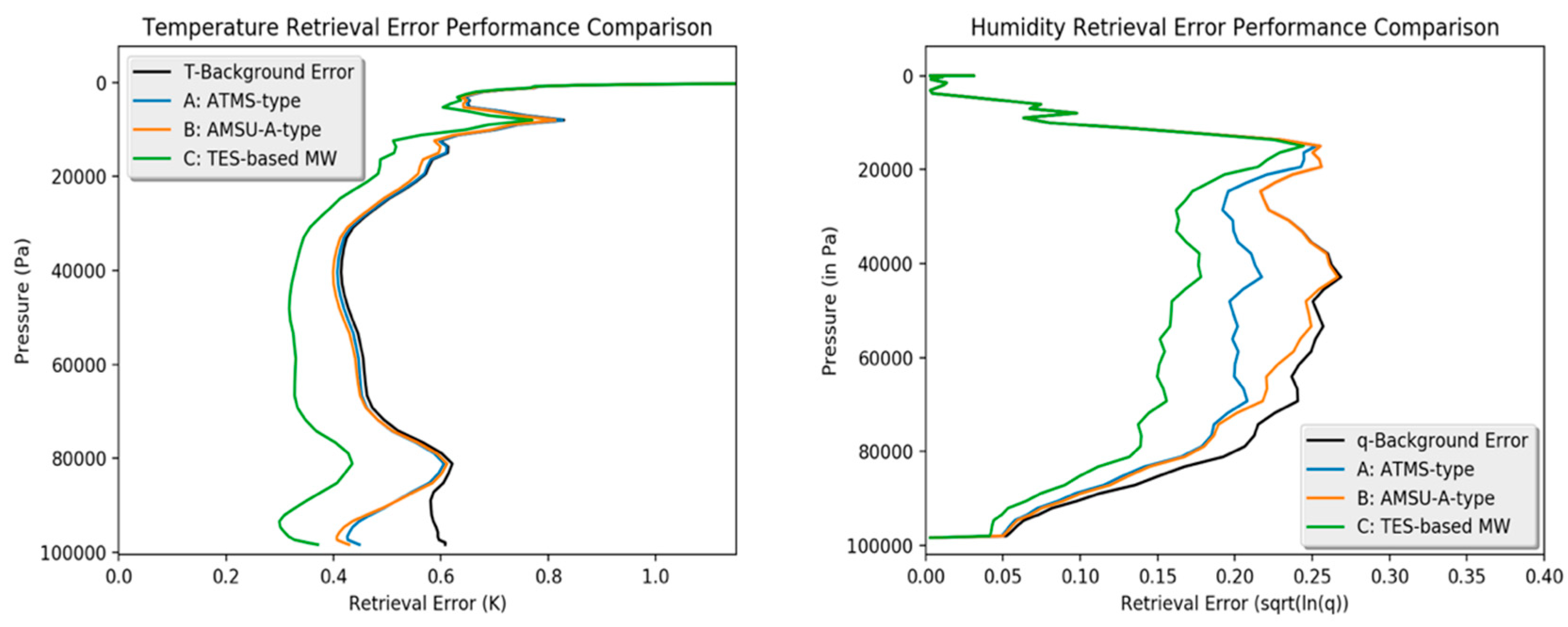
4.3.3. Retrieval Error Performance Simulations

The retrieval error performance of all the MW system configurations (A, B and C) was estimated using the information and error analysis model and these are presented in Figure 8. This shows the improvements of the ATMS-type, AMSU-A-type and TES-based MW instruments over the background errors for temperature and humidity. The results in Figure 8 show that a TES-based MW sounding instrument (configuration C) outperforms the other two configurations (A: ATMS-type and B: AMSU-A-type) for both temperature and humidity profiling.
The aforementioned improvements (as in Section 4.3.2) are mainly attributed to the TES-based MW instrument’s (configuration C) excellent NEDT performance. We have also observed that in the case of humidity retrieval, the ATMS-type instrument provides noticeable improvements compared to the AMSU-A-type instrument, due to the five additional 183 GHz humidity sounding channels. These results show the direct impact of instrument noise on the information content for each instrument. This also demonstrates the importance of achieving better instrument noise performance for improving the temperature and humidity retrievals.

5. Conclusions

A generic framework for an End-to-end Instrument Performance Simulation System (EIPS) for the satellite atmospheric remote sensing instruments has been developed and presented in this paper. The EIPS framework was derived from a systematic atmospheric observing system design (AOSD) process, as described in Rodgers [18]. This useful AOSD process was first visualised (as a schematic block diagram) in the paper and then taken as a reference guideline to build the framework. The EIPS has been built around the HT-FRTC (an atmospheric radiative transfer model) to form a complete simulation framework that can be used for instrument performance analysis and simulation tasks (such as trade-off analysis and design parameter optimisation). The design and the organisation of EIPS components (sensor parameter model, HT-FRTC model and the information and error analysis model) have been described. The EIPS framework offers fast radiative transfer simulation capability, any number of satellite remote sensing instruments can be simulated, and it is flexible to new and emerging technology-based sensors. To demonstrate the flexibility of the framework, a novel superconducting TES-based multi-spectral MW instrument has been presented as an example. In the last section of this paper, we further applied the EIPS framework by conducting a case study (as an example of framework’s application), in which we analysed the relative performance of three MW instrument configurations (A, B and C). The results on the relative performance of these three MW instrument configurations (two configurations (A and B) are based on existing multi-spectral MW instruments and the third configuration (C) is based on emerging technology) have been presented.
Configuration A and B were based on the existing ATMS and AMSU-A instruments respectively. Configuration C in this paper is based around recently emerging superconducting TES-based filterbank spectrometer technology. For the purposes of this paper, we modelled a relatively simple instrument with the same channel configuration as ATMS-type instrument (Configuration A), but with the greatly improved noise performance offered by this technology. EIPS experimental simulations have shown that when comparing configuration A and B, configuration B (an AMSU-A-type instrument) provided a relatively high information content on temperature as compared to configuration A (an ATMS-type instrument). This improvement can be mainly attributed to the low instrument noise in the temperature sounding channels of AMSU-A-type instrument. But, in the case of humidity, configuration A (ATMS-type) provided relatively more information compared to configuration B; this improvement is mainly because configuration A contains five extra humidity sounding channels around 183.31 GHz water vapour absorption line. While comparing all three configurations, we observed that configuration C (a TES-based MW instrument) provides the highest information content on temperature and humidity. As configuration C has exactly the same channel configuration as configuration A, this improvement in information content can be directly attributed to the much lower radiometric noise in each channels of configuration C. This demonstrates that the radiometric noise (NEDT) is an important factor in improving the retrieval error performance of the instrument.
The technology (on which the configuration C is based) offers greatly improved noise performance, and it allows the implementation of potentially thousands of sounding channels ranging from ~30 GHz up to ~850 GHz with very narrow spectral bandwidths. This opens up some very exciting new instrument concepts and sounding capabilities. The developed EIPS framework in this paper will be used for performance simulations and trade-off studies to find an optimal configuration for a hyperspectral MW instrument based on this emerging superconducting TES-based filterbank spectrometer technology, which will be the subject of our next paper. The EIPS framework will also be useful in trade studies where comparative assessments of large numbers of instrument configurations (with different system parameters such as: channels, bandwidth, spectral resolution, observation geometry etc.) are required. Furthermore, because of the EIPS framework’s applicability across the EM spectrum, it will be a useful tool for studies investigating the potential synergy between satellite atmospheric remote sensing instruments working in different parts of EM spectrum. An example of such a study is by Sato [31], in which the synergy between satellite remote sensing measurements at UV, IR and MW spectral ranges for the retrieval of vertical profiles of ozone have been investigated.
The EIPS framework is under continuous development to incorporate more functionalities. Some anticipated future developments include: radio frequency interference (RFI) mitigation algorithms, satellite data dimensionality reduction techniques such as the principal component analysis (PCA) and metrics for measuring instrument synergy studies are planned for integration into the framework.

Author Contributions

Conceptualisation P.K.D; Formal Analysis, P.K.D, S.H. and P.H.; Investigation, P.K.D, S.H. and P.H., Supervision, S.H., P.H., A.O., R.S., C.T., D.G., and S.W., Writing-original draft, P.K.D and Writing-review and editing, all the authors (P.K.D.,S.H., P.H., A.O., R.S., C.T., D.G. and S.W).

Acknowledgments

We are sincerely thankful to The Commonwealth Scholarship Commission in the UK (CSC) for Prateek Kumar Dongre’s research funding (CSC Reference Number: INCS-2016-214).

Conflicts of Interest

The authors declare no conflict of interest.

Abbreviations

The following abbreviations are used in this paper:
AMSU-AAdvanced Microwave Sounding Unit-A
AMSU-BAdvanced Microwave Sounding Unit-B
AOSDAtmospheric Observing System Design
ATMSAdvanced Technology Microwave Sounder
DFSDegrees of Freedom for Signal
ECMWFEuropean Centre for Medium-Range Weather Forecasts
EIPSEnd-to-End Instrument Performance Simulation System
EMElectromagnetic
HT-FRTCHavemann-Taylor Fast Radiative Transfer Code
IASIInfrared Atmospheric Sounding Interferometer
ICIIce Cloud Imager
IRInfraRed
MAPMaximum-a-posteriori
MetOpMeteorological Operational
MHSMicrowave Humidity Sounder
MWMicrowave
MWIMicroWave Imager
MWSMicroWave Sounder
NETDNoise Equivalent Temperature Difference
NWPNumerical Weather Prediction
OEOptimal Estimation
PCPrincipal Component
PCAPrincipal Component Analysis
SRFSpectral Response Function
TESTransition Edge Sensor
UMUnified Model
UVUltraviolet

References

  1. Joo, S.; Eyre, J.; Marriott, R. The Impact of MetOp and Other Satellite Data within the Met Office Global NWP System Using an Adjoint-Based Sensitivity Method. Mon. Weather Rev. 2013, 141, 3331–3342. [Google Scholar] [CrossRef]
  2. Geer, A.J.; Bauer, P. Observation errors in all-sky data assimilation. Q. J. R. Meteorol. Soc. 2011, 137, 2024–2037. [Google Scholar] [CrossRef]
  3. Zhu, Y.; Gelaro, R. Observation Sensitivity Calculations Using the Adjoint of the Gridpoint Statistical Interpolation (GSI) Analysis System. Mon. Weather Rev. 2008, 136, 335–351. [Google Scholar] [CrossRef]
  4. Cardinali, C. Monitoring the observation impact on the short-range forecast. Q. J. R. Meteorol. Soc. 2009, 135, 239–250. [Google Scholar] [CrossRef]
  5. Collard, A.D.; McNally, A.P. The assimilation of Infrared Atmospheric Sounding Interferometer radiances at ECMWF. Q. J. R. Meteorol. Soc. 2009, 135, 1044–1058. [Google Scholar] [CrossRef]
  6. Radnóti, G.; Bauer, P.; McNally, A.; Cardinali, C.; Healy, S.; de Rosnay, P. ECMWF Study on the Impact of Future Developments of the Space-Based Observing System on Numerical Weather Prediction. ECMWF. December 2010. Available online: https://www.ecmwf.int/en/elibrary/11815-ecmwf-study-impact-future-developments-space-based-observing-system-numerical (accessed on 26 March 2019).
  7. McNally, A. Observing System Experiments to Assess the Impact of Possible Future Degradation of the Global Satellite Observing Network. ECMWF. March 2012. Available online: https://www.ecmwf.int/en/elibrary/11085-observing-system-experiments-assess-impact-possible-future-degradation-global (accessed on 26 March 2019).
  8. McNally, T.; Bonavita, M.; Thépaut, J.-N. The Role of Satellite Data in the Forecasting of Hurricane Sandy. Mon. Weather Rev. 2014, 142, 634–646. [Google Scholar] [CrossRef]
  9. English, S.J.; McNally, A.; Bormann, N.; Salonen, K.; Matricardi, M.; Horányi, A.; Rennie, M.; Janiskova, M.; Di Michele, S.; Geer, A.; et al. Impact of Satellite Data. ECMWF. October 2013. Available online: https://www.ecmwf.int/en/elibrary/9301-impact-satellite-data (accessed on 26 March 2019).
  10. Lerner, J.A. Temperature and humidity retrieval from simulated Infrared Atmospheric Sounding Interferometer (IASI) measurements. J. Geophys. Res. 2002, 107. [Google Scholar] [CrossRef] [Green Version]
  11. Rosenkranz, P.W. Retrieval of temperature and moisture profiles from AMSU-A and AMSU-B measurements. IEEE Trans. Geosci. Remote Sens. 2001, 39, 2429–2435. [Google Scholar] [CrossRef]
  12. Pearson, K.; Merchant, C.; Embury, O.; Donlon, C. The Role of Advanced Microwave Scanning Radiometer 2 Channels within an Optimal Estimation Scheme for Sea Surface Temperature. Remote Sens. 2018, 10, 90. [Google Scholar] [CrossRef]
  13. Kangas, V.; D’Addio, S.; Betto, M.; Barre, H.; Mason, G. MetOp Second Generation Microwave radiometers. In Proceedings of the 2012 12th Specialist Meeting on Microwave Radiometry and Remote Sensing of the Environment (MicroRad), Rome, Italy, 5–9 March 2012; pp. 1–4. [Google Scholar]
  14. Alberti, G.; Memoli, A.; Pica, G.; Santovito, M.R.; Buralli, B.; Varchetta, S.; D’addio, S.; Kangas, V. TWO Microwave Imaging radiometers for MetOp Second Generation. In Proceedings of the 2012 Tyrrhenian Workshop on Advances in Radar and Remote Sensing (TyWRRS), Naples, Italy, 12–14 September 2012; pp. 243–246. [Google Scholar]
  15. Bizzarri, B.; Gasiewski, A.; Staelin, D. Initiatives for millimetre/submillimetre-wave sounding from geostationary orbit. In Proceedings of the IEEE International Geoscience and Remote Sensing Symposium, Toronto, ON, Canada, 24–28 June 2002; Volume 1, pp. 548–552. [Google Scholar]
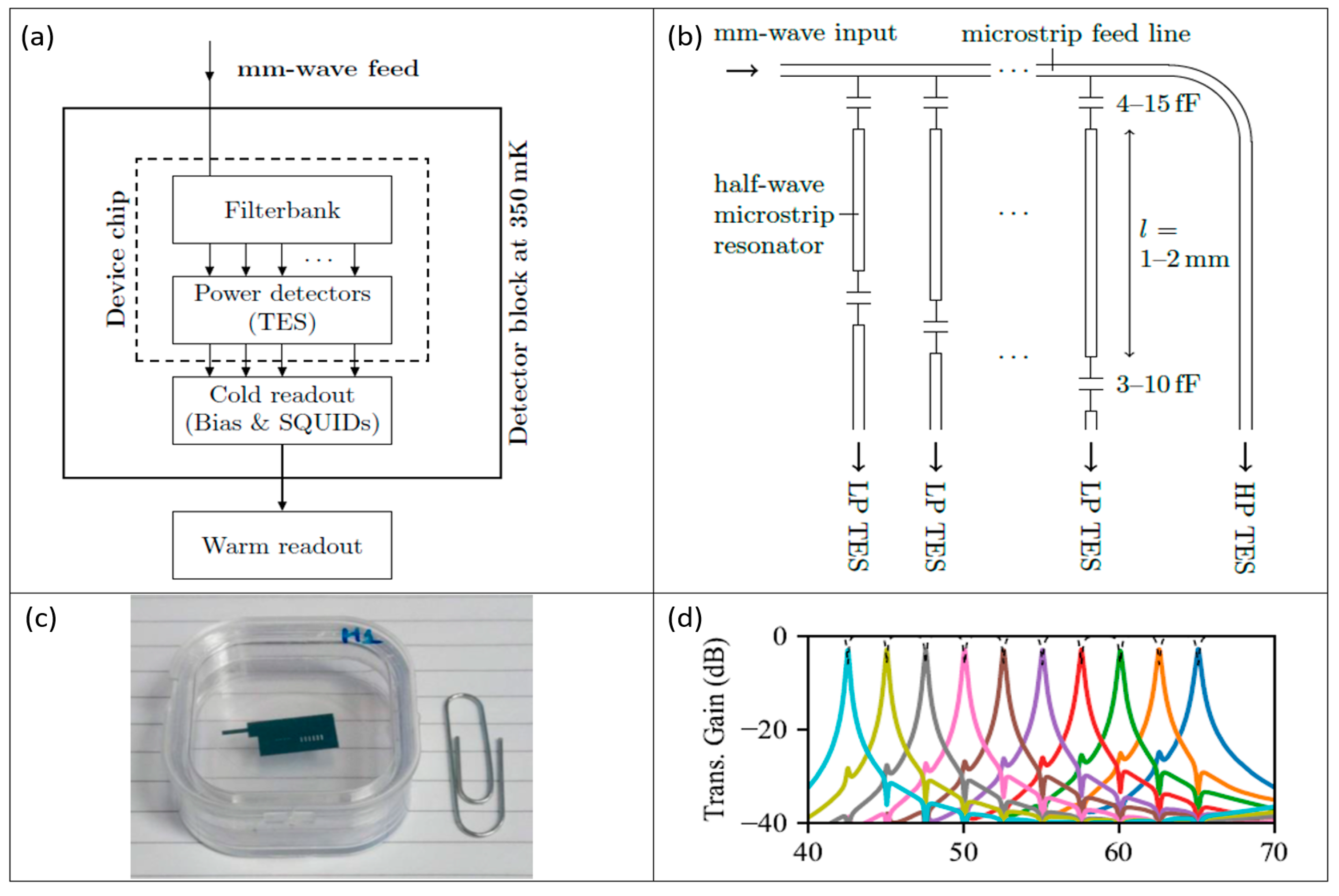
  16. Thomas, C.; Goldie, D.J.; Withington, S.; Hargrave, P.; Orlando, A.; Sudiwala, R.; Dongre, P.K. Transition Edge Sensor Superconducting Filterbank Spectrometers for Hyperspectral Microwave Atmospheric Sounding. In Proceedings of the 8th ESA Workshop on Millimetre-Wave Technology and Applications (in press); ESA-ESTEC, Noordwijk, The Netherlands, 10–12 December 2018; p. Session 5A. [Google Scholar]
  17. McMillin, L.M.; Fleming, H.E. Trade-Offs in the Design of Satellite Sounding Instruments. J. Atmospheric Ocean. Technol. 1985, 2, 278–284. [Google Scholar] [CrossRef] [Green Version]
  18. Rodgers, C.D. Inverse Methods for Atmospheric Sounding: Theory and Practice; Series on Atmospheric, Oceanic and Planetary Physics; World Scientific: Singapore, 2000; Volume 2, ISBN 978-981-02-2740-1. [Google Scholar]
  19. Havemann, S.; Thelen, J.-C.; Taylor, J.P.; Harlow, R.C. The Havemann-Taylor Fast Radiative Transfer Code (HT-FRTC): A multipurpose code based on principal components. J. Quant. Spectrosc. Radiat. Transf. 2018, 220, 180–192. [Google Scholar] [CrossRef]
  20. Newman, S.M.; Clarisse, L.; Hurtmans, D.; Marenco, F.; Johnson, B.; Turnbull, K.; Havemann, S.; Baran, A.J.; O’Sullivan, D.; Haywood, J. A case study of observations of volcanic ash from the Eyjafjallajökull eruption: 2. Airborne and satellite radiative measurements: Eyjafjallajökull radiative case study. J. Geophys. Res. Atmos. 2012, 117. [Google Scholar] [CrossRef]
  21. Athanassiadou, M.; Francis, P.N.; Saunders, R.W.; Atkinson, N.C.; Hort, M.C.; Havemann, S.; Thelen, J.-C.; Bush, M. A case study of sulphur dioxide identification in three different volcanic eruptions, using Infrared satellite observations (IASI): Volcanic SO 2 detection from IASI. Meteorol. Appl. 2016, 23, 477–490. [Google Scholar] [CrossRef]
  22. Aumann, H.H.; Chen, X.; Fishbein, E.; Geer, A.; Havemann, S.; Huang, X.; Liu, X.; Liuzzi, G.; DeSouza-Machado, S.; Manning, E.M.; et al. Evaluation of Radiative Transfer Models with Clouds. J. Geophys. Res. Atmos. 2018, 123, 6142–6157. [Google Scholar] [CrossRef]
  23. Baran, A.J.; Furtado, K.; Labonnote, L.-C.; Havemann, S.; Thelen, J.-C.; Marenco, F. On the relationship between the scattering phase function of cirrus and the atmospheric state. Atmos. Chem. Phys. 2015, 15, 1105–1127. [Google Scholar] [CrossRef] [Green Version]
  24. Thelen, J.-C.; Havemann, S.; Taylor, J.P. Atmospheric Correction of Short-Wave Hyperspectral Imagery Using a Fast, Full-Scattering 1DVar Retrieval Scheme; Shen, S.S., Lewis, P.E., Eds.; SPIE: Baltimore, MD, USA, 2012; p. 839010. [Google Scholar]
  25. Gristey, J.J.; Chiu, J.C.; Gurney, R.J.; Shine, K.P.; Havemann, S.; Thelen, J.-C.; Hill, P.G. Short-wave spectral radiative signatures and their physical controls. J. Clim. 2019. [Google Scholar] [CrossRef]
  26. Smith, F.; Havemann, S.; Hoffmann, A.; Bell, W.; Weidmann, D.; Newman, S. Evaluation of laser heterodyne radiometry for numerical weather prediction applications. Q. J. R. Meteorol. Soc. 2018, 144, 1831–1850. [Google Scholar] [CrossRef] [Green Version]
  27. Matricardi, M. The Generation of RTTOV Regression Coefficients for IASI and AIRS Using a New Profile Training Set and a New Line-by-Line Database. ECMWF. May 2008. Available online: https://www.ecmwf.int/en/elibrary/11040-generation-rttov-regression-coefficients-iasi-and-airs-using-new-profile-training (accessed on 26 March 2019).
  28. Ide, K.; Courtier, P.; Ghil, M.; Lorenc, A.C. Unified Notation for Data Assimilation: Operational, Sequential and Variational (gtSpecial IssueltData Assimilation in Meteology and Oceanography: Theory and Practice). J. Meteorol. Soc. Jpn. Ser. II 1997, 75, 181–189. [Google Scholar] [CrossRef]
  29. Smith, F.I. Improving the Information Content of IASI Assimilation for Numerical Weather Prediction. Ph.D. Thesis, University of Leicester, Leicester, UK, 2015. [Google Scholar]
  30. Eyre, J.R.; Hilton, F.I. Sensitivity of analysis error covariance to the mis-specification of background error covariance. Q. J. R. Meteorol. Soc. 2013, 139, 524–533. [Google Scholar] [CrossRef]
  31. Sato, T.O.; Sato, T.M.; Sagawa, H.; Noguchi, K.; Saitoh, N.; Irie, H.; Kita, K.; Mahani, M.E.; Zettsu, K.; Imasu, R.; et al. Vertical profile of tropospheric ozone derived from synergetic retrieval using three different wavelength ranges, UV, IR, and microwave: Sensitivity study for satellite observation. Atmos. Meas. Tech. 2018, 11, 1653–1668. [Google Scholar] [CrossRef]
Figure 1. Schematic of a superconducting filterbank based on transition-edge superconducting detector technology. (a) Overall filterbank architecture. (b) Schematic of filterbank—half-wave resonator coupled to feedline and TES detector. (c) Prototype 10-channel low spectral resolurion (R=200) device chip. (d) Modelled filter response (R=200). Figures from Thomas et al. [16].
Remotesensing 11 01412 g001
Figure 2. A flow-diagram for the visualisation of the process of design and optimisation of a satellite atmospheric observing system via end-to-end simulation.
Remotesensing 11 01412 g002
Figure 3. A schematic block diagram of the EIPS Framework, showing three important component models of the framework.
Remotesensing 11 01412 g003
Figure 4. Comparison of fast and line mode of the EIPS framework radiative transfer model, the HT-FRTC: (a) Brightness temperature bias (calculated for fast code compared with the line HT-FRTC code). (b) Brightness temperature standard deviation between fast and line HT-FRTC code.
Remotesensing 11 01412 g004
Figure 5. Flow diagram showing the process of reconstruction of instrument simulated spectra by the convolution of very high spectrally resolved radiances with instrument spectral response function.
Remotesensing 11 01412 g005
Figure 6. Simulated temperature and humidity Jacobians for two MW instrument configurations (A and B): Temperature and Humidity Jacobians for configuration A (ATMS-type) (shown in two figures in the top panel) and for configuration B (AMSU-A-type) (shown in side-by-side two figures in the bottom panel).
Remotesensing 11 01412 g006
Figure 7. Estimated averaging kernel matrices (using Equation (8)) for temperature and humidity for all the MW system configurations considered in this case study: A (ATMS-type) (top), B (AMSU-A) (middle) and C (TES-based MW) (bottom) calculated using EIPS information and error analysis model. In these presented contour plots of averaging kernel matrices (for temperature and humidity), the “model levels” refers to the 70 Met Office UM model levels as mentioned in Section 4.1.
Remotesensing 11 01412 g007
Figure 8. Temperature (in left) and Humidity (in right) retrieval error performance estimation and comparison for all three MW instrument system configurations (A (ATMS-type), B (AMSU-A-type) and C (TES-based MW)).
Remotesensing 11 01412 g008
Table 1. End-to-End simulation settings for three MW instrument configurations set up.
System ParametersSettings
Geometrical configurationSensor zenith angle 53 degree,
fixed single field of view is considered
Spectral Range23 GHz- 183 GHz
(for all the configurations A, B and C)
Table 2. Spectral and radiometric specifications of set up MW system configurations A, B and C.
Centre Frequency
(GHz)
Bandwidth (MHz)ApplicationNETD of MW System Configurations (K)
(A)
ATMS-Type
(B)
AMSU-A-Type
(C)
TES-Based MW
23.8 *270Window-Water vapour0.90.30.025
31.4 *180Window-water vapour 0.90.30.038
50.3 *180Window-surface emissivity1.20.40.038
51.7400Window-surface emissivity 0.750.250.017
52.8 *400Temperature0.750.250.017
53.596 ± 0.115 *1700.750.250.041
54.40 *4000.750.250.017
54.94 *4000.750.250.017
55.50 *3300.750.250.021
57.290344 *3300.750.250.021
57.290344 ± 0.217 *781.200.400.089
57.290344 ± 0.3222 ± 0.048 *361.200.400.192
57.290344 ± 0.3222 ± 0.022 *161.500.600.433
57.290344 ± 0.3222 ± 0.010 *82.400.800.865
57.290344 ± 0.3222 ± 0.0045 *33.601.202.308
89.0 *6000Window0.500.50
89.550000.50 0.001
165.53000Water-vapour0.60 0.002
183.31 ± 7.020000.80 0.004
183.31 ± 4.520000.80 0.004
183.31 ± 3.010000.80 0.007
183.31 ± 1.810000.80 0.007
183.31 ± 1.05000.90 0.014
* AMSU-A-type (Configuration B) instrument channels and corresponding bandwidths.
Table 3. Information Content (DFS) Estimations.
MW System ConfigurationAverage DFS
(Over Eight Atmospheric Profiles)
Temperature (T)Humidity (q)
A0.352.24
B1.150.67
C6.275.29

