An Energy-Based SAR Image Segmentation Method with Weighted Feature

Abstract

To extract more structural features, which can contribute to segment a synthetic aperture radar (SAR) image accurately, and explore their roles in the segmentation procedure, this paper presents an energy-based SAR image segmentation method with weighted features. To precisely segment a SAR image, multiple structural features are incorporated into a block- and energy-based segmentation model in weighted way. In this paper, the multiple features of a pixel, involving spectral feature obtained from original SAR image, texture and boundary features extracted by a curvelet transform, form a feature vector. All the pixels’ feature vectors form a feature set of a SAR image. To automatically determine the roles of the multiple features in the segmentation procedure, weight variables are assigned to them. All the weight variables form a weight set. Then the image domain is partitioned into a set of blocks by regular tessellation. Afterwards, an energy function and a non-constrained Gibbs probability distribution are used to combine the feature and weight sets to build a block-based energy segmentation model with feature weighted on the partitioned image domain. Further, a reversible jump Markov Chain Monte Carlo (RJMCMC) algorithm is designed to simulate from the segmentation model. In the RJMCMC algorithm, three move types were designed according to the segmentation model. Finally, the proposed method was tested on the SAR images, and the quantitative and qualitative results demonstrated its effectiveness.

1. Introduction

Image segmentation is a hot topic in the date processing of a synthetic aperture radar (SAR) image [1,2]. In the traditional image segmentation method, homogeneous regions are segmented according to spectral features of pixels [3]. With the rapid development of SAR technology, the resolution of a SAR image is also getting higher and higher. Compared with the middle and low resolution SAR images, the details of high resolution SAR images becomes clearer, but the differences between homogeneous regions becomes larger, and the differences between heterogeneous regions becomes smaller simultaneously [4]. These causes the traditional segmentation method to not reach the segmentation accuracy of a high resolution SAR image [5]. Therefore, high resolution SAR image segmentation becomes a difficult and hot topic. The differences among homogeneous regions in the high resolution SAR image exist not only in spectral features, but also in structural features such as boundary and texture features [6]. To segment a high resolution SAR image well, multiple structural features can be considered in the segmentation algorithm [7,8,9].

For example, Liu et al. [10] presents a SAR image segmentation method using contourlet transform and support vector machine (SVM). This method utilizes contourlet transform to define the energy, standard deviation and information entropy, and these features are used to construct the texture feature vector; Then SVM is used to segment the SAR image based on the texture feature vector. Xue et al. [11] proposes a method of SAR image segmentation based on fuzzy c-means (FCM) and wavelet transform. In this paper, the vector composed by wavelet texture features and the gray level of a SAR image filtered, on the basis, FCM is used to segment a SAR image. Hao et al. [12] presents a SAR segmentation method based on a maximization of posterior marginals (MPM) algorithm with feature extraction and context model. In this method, a Gabor wavelet and texture descriptor are used to extract features, and the MPM of each region combined with the context model is utilized to segment a SAR image. All the above methods use multiple features to segment an image, but in segmentation procedure, the roles of features are considered as the same. However, they are not necessarily the same actually. With the development of deep learning technology, Lv et al. [13] proposes a feature learning method using a stacked contractive autoencoder (sCAE) to extract the temporal change feature for a SAR image. First, an affiliated temporal change image is built by three different metrics; then the simple linear iterative clustering algorithm is utilized to generate superpixels; and a sCAE network is trained with the superpixel samples as an input to learn the change features in semantic; finally, the encoded features by this sCAE model are binary segmented to create the change result map. Although deeper leaning can segment a SAR image better, it needs much time to train before the segmentation, it reduces the efficiency.

To extract more structural features that can contribute to segmenting accurately and explore the roles of features in the segmentation procedure, this paper presents a feature weighted SAR image segmentation method based on the energy function. As spectral, texture and boundary features are three basis features of a SAR image, they are good for segmenting, so these three features of a pixel are used to form a feature vector, and all the feature vectors form a feature set. To automatically determine the roles of the features in the segmentation procedure, weight variables are defined, and all the weight variables form a weight set. Afterwards, the feature and weight sets are combined to build a feature weighted segmentation model by using an energy function and a non-constrained Gibbs probability distribution. Further, a reversible jump Markov Chain Monte Carlo (RJMCMC) algorithm is used to simulate from the segmentation model. Finally, the proposed method is tested on the SAR images to demonstrate its effectiveness. Image segmentation is a prelude for further SAR image processing tasks such as feature extraction [14], object recognition [15] and classification [16], so the proposed method can be used to detect an oil dark spot, extract its features and so on.

This paper is organized as follows. Section 2 presents the proposed algorithm. Section 3 details the results of simulated and real SAR images. Section 4 discusses the test results; Finally, Section 5 contains conclusions and perspectives for further research.

2. Materials and Methods

Given a SAR image f = {f_s = f(r_s, c_s); s = 1, …, S}, where s is pixel index; r_s ∈ {1, …, m₁} is the row of pixel s, c_s ∈ {1, …, m₂} is the column of pixel s, m₁ and m₂ are the number of rows and columns in the SAR image, respectively; (r_s, c_s) is the location of pixel s; f_s is the intensity of pixel s, it represents the spectral feature of pixel s in this paper; S is the total number of pixels in the SAR image, and can be expressed as S = m₁ ’ m₂; P = {(r_s, c_s); s =1, …, S} is a set of locations for all the pixels in the SAR image (short for image domain).

2.1. Curvelet Transform

The second generation curvelet transform is defined in both the continuous and discrete domain, and in image processing the most commonly used one is its discrete representation. The discrete curvelet transform takes a 2D image f as an input in the form of a Cartesian array f(r_s, c_s). As shown in Equation (1), the outputs of the discrete curvelet transform are a collection of digital curvelet coefficients C^D(j, l, k). That is, the digital curvelet coefficients C^D(j, l, k) are simply the inner product between a 2D image f and a digital curvelet ${\varphi }_{j,l,k}^D$ [17].

$$C^D(j,l,k):=\langle f,{\varphi }_{j,l,k}^D\rangle ={\displaystyle \sum _{\begin{array}{l}{r}_s\in \{1,\dots ,m_1\}\\ c_s\in \{1,\dots ,m_2\}\end{array}}f(r_s,c_s){\varphi }_{j,l,k}^D(r_s,c_s)}$$

(1)

where D stands for “digital”; < ⋅ > represents the inner operation; l is orientation (angle) parameter; k = (k₁, k₂) ∈ R² is the sequence of translation parameters; ⌈ ⋅ ⌉ stands for ceil operation; j∈ {1, …, J} is a scale parameter, J is the number of scales; when j = 1, the coarse scale coefficients C^D(1, l, k) are low frequency coefficients, they include the main information of the SAR image; when j = J, the finest coefficients C^D(J, l, k) are high frequency coefficients, they include much detailed information of the SAR image, such as the information of speckle noise; when j ∈ {2, J − 1}, the detail coefficients C^D(j, l, k) are middle-high frequency coefficients, they include much of the boundary information of the SAR image [17].

There are two different digital implementation of the second generation curvelet transforms, this paper uses the wrapping based on the curvelet transform [17], and whose architecture is then roughly as follows.

(1) For a given SAR intensity image f = {f_s = f(r_s, c_s); s = 1, …, S}, the 2D fast Fourier transform (FFT) is applied and Fourier samples $\widehat{f}[n_1,n_2]$ can be obtained, where n₁ and n₂ are frequency domain variables, – r_s /2 ≤ n₁, n₂ ≤ c_s /2;

(2) For each scale j and angle l, the frequency window $\widetilde{U_{j,l}}[n_1,n_2]$ and Fourier samples $\widehat{f}[n_1,n_2]$ are multiplied to form the product $\widetilde{U_{j,l}}[n_1,n_2]\widehat{f}[n_1,n_2]$ is constructed;

(3) Wrapping this product around the origin, the corresponding periodization of this product $W\left(\widetilde{U_j},\widehat{f_{j,l}}\right)[n_1,n_2]$ can be obtained, where (n₁, n₂)∈ρ_j, ρ_j ={(n₁, n₂), n₁∈[0, L_{1, j}], n₂∈[0, L_{2, j}]} is a rectangle with sides of length L_{1, j} × L_2,j near the origin, L_{1, j} ≈ 2^j, L_{2, j} ≈ 2^j/2;

(4) The inverse 2D FFT is applied to obtain the discrete coefficients C^D(j, l, k).

2.2. Feature Extraction

The differences among homogeneous regions of a SAR image exist not only in spectral features, but also in structural features, such as boundary, texture features and so on. In order to accurately segment homogeneous regions, spectral, texture and boundary features are used in the proposed segmentation method. In this paper, a spectral feature is the original SAR image f, and texture and boundary features are extracted by curvelet transform.

Texture feature is a basic image feature and good for segmentation. In this paper, curvelet transform and L₁ norm are used to define energy, which is considered as a texture feature. The larger the energy is, the more the texture information is [18]. The operation is as follows. First, the curvelet transform is used to decompose a sub-image with c_t × c_t pixels centered on pixel s to obtain a series of curvelet coefficients. Then L₁ norm is used to define the energy of pixel s can be computed [18],

$$x_{ts}=\frac{1}{N_t}{\displaystyle \sum _{j,l,k}|C^D(j,l,k){|}^2}$$

(2)

where N_t is the total number of curvelet coefficients. In accordance with the above procedure, the texture feature of the SAR image x_t = {x_ts; s = 1, …, S} is obtained.

Boundary is another basic feature, which is also an important factor to divide different homogeneous regions. As a common boundary detection algorithm, a Canny operator [19] can better extract the boundary features in an optical image. However, a Canny operator can not accurately extract the boundary features of a SAR image, it drives from the effect of speckle noise. In this paper, curvelet transform and a Canny operator are used to define the feature. The operation is as follows. Firstly, the curvelet transform is used to decompose the SAR image f to obtain a series of curvelet coefficients. As the detail coefficients C^D(j, l, k) (j ∈ {2, J − 1}) are middle-high frequency coefficients, they include much of the boundary information of the SAR image. Therefore, the detail coefficients are unchanged, a Canny operator is just used for extracting the boundary of curvelet coefficients on the coarse and finest scales, and their non-boundary curvelet coefficients are changed to 0. That is, all the boundary curvelet coefficients are unchanged and all the non-boundary curvelet coefficients are changed to 0. Finally, all the curvelet coefficients are reconstructed to obtain the boundary feature of the SAR image x_b = {x_bs; s = 1, …, S},

$$x_b={\displaystyle \sum _{j,l,k}{C}^D(j,l,k){\varphi }_{j,l,k}^D}$$

(3)

In summary, a feature set of the SAR image is composed by the original spectral, extracted texture and boundary features, that is, x = {f, x_t, x_b} = {x_s; s = 1, …, S} = {x_gs; g = 1, …, G, s = 1, …, S}, where x_s is the feature vector values of pixel s, g is feature index, x_gs is g^th feature value of pixel s. x can be considered as a realization of a random feature filed X = {X_s; s = 1, …, S} defined on the image domain P, where X_s is the feature vector of pixel s, that is, X_s = {X_gs; g = 1, …, G}, X_gs is g^th feature variable of pixel s.

2.3. Energy-based Segmentation Model with Feature Weighted

In order to automatically determine the roles of the multiple features in the segmentation procedure, a weight variable ${\omega }_{g{y}_s}$ is assigned to a variable of a pixel’s feature vector X_gs in the X_s. All the weight variables form a weight set, that is, ω = {${\omega }_{g{y}_s}$; g = 1, …, G, s = 1, …, S}, where y_s is the label of pixel s.

As the effect of speckle noise in the SAR image, the traditional segmentation method based on pixel can not segment well in the homogeneous regions. To improve the segmentation accuracy in the homogeneous regions, the sub-region is considered as a processing unit, that is, an image domain is partitioned by the geometric partitioning technique, and region-based statistic models are built on the partitioned image domain. As the principle of regular tessellation is simple and easy to be realized, it is explored for partitioning P into a set of rectangle regular blocks (short for blocks), that is, P = {P_i; i = 1, …, I}, where i is the index of block; I is the total number of blocks, and considered as a random variable; P_i is the ith block, the number of pixels in P_i is the multiple of two and the minimum block is 2 × 2. The initial image domain can be partitioned by S/m² blocks, where the initial value of I = S/m², the number of pixels in every block is m × m, where m is greater than or equal to two, and m can split r_s and c_s. It has been selected by many experiments that the initial value of m = 8 in this paper. The number of blocks and the sizes of blocks will be changed by the following move of sampling the number of blocks.

On the partitioned image domain, the partitioned blocks are considered as processing units, it means that the labels of pixels in a block are the same, and their weights are also the same. Therefore, the weight set can be rewritten as ω = {${\omega }_{g{y}_i}$; g = 1, …, G, i = 1, …, I} = {ω_go; g = 1, …, G, o = 1, …, O}, where ω_go is the weight variable of label o on the g^th feature, O is the total number of classes and regarded as known, y_i is the label of block P_i.

All the labels form a realization of a label field, that is, y = {y_i; i = 1, …, I}, which represents attributes of blocks to different classes, and corresponds to a segmentation of the feature set x. This paper uses the energy function of a neighborhood relationship to build the model of label field [20], it can be expressed as:

$$U_y(y,I)={\displaystyle \sum _{i=1}^I\left\{-\gamma \left[{\displaystyle \sum _{P_r\in N{P}_i}2\delta (y_i,y_r)-1}\right]\right\}}$$

(4)

where γ is a constant to control the neighborhood dependences between a pair of neighbor blocks; NP_i ={ P_r; P_i ~ P_r} is the set of P_i’s neighbor blocks, i, r ∈ {1, …, I} and i ≠ r, P_i ~ P_r are neighbors if and only if they have a mutual boundary; if y_i = y_r, the indictor function δ(y_i, y_r) = 1, otherwise, δ(y_i, y_r) = 0.

The model of weighted feature U_x(x, ω) can be written as:

$$U_x(x,\omega ,I)={\displaystyle \sum _{i=1}^I{U}_x(x_i,{\omega }_i)={\displaystyle \sum _{i=1}^I{\displaystyle \sum _{g=1}^G{U}_x(x_{gi},{\omega }_{gi})}}}$$

(5)

where

$$U_x(x_{gi},{\omega }_{gi})=V(x_{gi},x_{g{y}_i})-\log ({\omega }_{g{y}_i})$$

(6)

where x_gyi = {x_gi; i ∈ P_yi}; P_yi is the set of the blocks belonging to the label y_i; V(x_gi, x_gyi) is heterogeneous energy function and defined by K-S distance [18], it can be expressed as

$$V(x_{gi},x_{g{y}_i})=d_{KS}(x_{gi},x_{g{y}_i})=\underset{h}{\max }\left|{\widehat{F}}_{x_{gi}}(h)-{\widehat{F}}_{x_{g{y}_i}}(h)\right|$$

(7)

where d_KS is K-S distance, that is, the maximum distance between ${\widehat{F}}_{x_{gi}}$ and ${\widehat{F}}_{x_{g{y}_i}}$, ${\widehat{F}}_{x_{gi}}$ and ${\widehat{F}}_{x_{g{y}_i}}$ are cumulative sampling distribution of x_gi and x_gyi, respectively. ${\widehat{F}}_{x_{gi}}$ and ${\widehat{F}}_{x_{g{y}_i}}$ can be written as [21]:

$${\widehat{F}}_{x_{gi}}(h)=\frac{1}{n_1}\#\{s|x_{gs}\le h\}$$

(8)

$${\widehat{F}}_{x_{g{y}_i}}(h)=\frac{1}{n_2}\#\{s|x_{g{y}_i}\le h\}$$

(9)

where # is an operation that returns the number of elements in the set, n₁ and n₂ are the total number of elements x_gi and x_gyi, respectively; h is the index of feature values; For a H bit image, h ∈ {0, 2^H − 1}.

In the statistic segmentation, a complete segmentation model not only models the features of the image, but also describes the attributes of pixels to different classes [22]. To fully utilize the roles of the label field, the feature field and weight set in the segmentation procedure, a global energy function of image segmentation is defined by the label model and feature weighted model, it can be expressed as:

$$\begin{array}{l}U(x,\omega ,y,I)=U_y(y,I)+U_x(x,\omega ,I)\\ ={\displaystyle \sum _{i=1}^I\left\{-\gamma \left[{\displaystyle \sum _{P_r\in N{P}_i}2\delta (y_i,y_r)-1}\right]\right\}}+{\displaystyle \sum _{i=1}^I{\displaystyle \sum _{g=1}^G\left[V(x_{gi},x_{g{y}_i})-\log ({\omega }_{g{y}_i})\right]}}\end{array}$$

(10)

In summary, the process of solving ω, y, I given x can be computed as:

$$(\widehat{\omega },\widehat{y},\widehat{I})=\min U(x,\omega ,y,I)$$

(11)

To incorporate the solving process of Equation (11) into the Bayesian statistical framework, non-constrained Gibbs probability distribution is used to describe the global energy function,

$$\begin{array}{l}G(x,\omega ,y,I)=\frac{1}{Z}\exp \{-U(x,\omega ,y,I)\}\\ =\frac{1}{Z}{\displaystyle \prod _{i=1}^I\left\{\exp \left\{\gamma \left[{\displaystyle \sum _{P_r\in N{P}_i}2\delta (y_i,y_r)-1}\right]\right\}\times {\displaystyle \prod _{g=1}^G\left\{{\omega }_{g{y}_i}\exp \left[-V(x_{gi},x_{g{y}_i})\right]\right\}}\right\}}\end{array}$$

(12)

where Z is a normalization constant.

2.4. Simulation

According to Equation (12), Let the total parameter vector Θ = (Y, I, ω). To solve their values, it is necessary to simulate from the energy-based segmentation model with the feature weighted. A RJMCMC algorithm is designed to generate samplers from Θ. In each iteration, a new candidate Θ^* for Θ is drawn from a proposal distribution with density q(Θ,Θ^*) (assume that the dimension of Θ^* is higher than that of Θ). u is a random vector defined for accomplishing a transition from (Θ, u) to Θ^* with dimension matching, that is, |Θ| + |u| = |Θ*|. The probability of accepting the candidate Θ^* can be computed as [23]:

$$a(\Theta ,{\Theta }^{*})=\min \left\{1,\frac{p({\Theta }^{*}|X)r({\Theta }^{*})}{p(\Theta |X)r(\Theta )q(u)}\left|\frac{\partial ({\Theta }^{*})}{\partial (\Theta ,u)}\right|\right\}$$

(13)

where q(u) is the density function of u, r(Θ) and r(Θ^*) are the probabilities of a given move type in the states Θ and Θ^*, respectively. The Jacobian | ∂(Θ^*) /∂(Θ, u)| derives from the change of variable from (Θ, u) to Θ^*.

(1) Sampling label field. A block P_i with the corresponding label y_i is randomly chosen. To update the label, a new label y_i^* is randomly drawn from {1, …, O} and y_i^* ≠ y_i. The acceptance probability can be written as:

$$a_o(y_i,y_i^{*})=\min \{1,R_o\}$$

(14)

where

$$R_o=\frac{{\displaystyle \prod _{g=1}^G\left\{{\omega }_{g{y}_i}\exp \left[-V(x_{gi},x_{g{y_i}^{*}})\right]\right\}}}{{\displaystyle \prod _{g=1}^G\left\{{\omega }_{g{y}_i}\exp \left[-V(x_{gi},x_{g{y}_i})\right]\right\}}}\times \frac{{\displaystyle \prod _{i=1}^I\exp \left\{\gamma \left[{\displaystyle \sum _{P_r\in N{P}_i}2\delta (y_i^{*},y_r)-1}\right]\right\}}}{{\displaystyle \prod _{i=1}^I\exp \left\{\gamma \left[{\displaystyle \sum _{P_r\in N{P}_i}2\delta (y_i,y_r)-1}\right]\right\}}}$$

(15)

Random number z is uniformly drawn from [0,1], that is, z ~ U[0,1]; if z ≤ a_o(y_i, y_i ^*), the result of the move is accepted, and y_i becomes y_i ^*; otherwise, the result of the move is rejected, and y_i is unchanged.

(2) Sampling the number of blocks. The operation is achieved by splitting or merging blocks, where the splitting move is an operation in which a block is split into two blocks with different class labels. The operation includes: (i) A block P_i is randomly chosen in the current partition of image domain P = {P₁, …, P_i, …, P_I}, and its corresponding label is o; (ii) If the pixel number of P_i is more than four and the number of its row or column is the multiple of two, P_i can be split. Under the constraint of minimum blocks, splitting types can be determined. (iii) One splitting is randomly chosen and splits P_i into P_i^* and P_I+1^*, and their corresponding labels are re-allocated y_i and y_i ^*, y_i ≠ y_i ^*, respectively. The new partition of the image domain becomes P^* = {P₁, …, P_i^*, …, P_I, P_I+1^*}, the acceptance probability of the splitting move can be expressed as:

$$a_{f_I}(P,P^{*})=\min \left\{1,R_{f_I}\right\}$$

(16)

where

$$\begin{array}{l}{R}_{f_I}=\\ \frac{{\displaystyle \prod _{i=1}^{I+1}{\displaystyle \prod _{g=1}^G\left\{{\omega }_{g{y}_i}\exp \left[-V(x_{gi},x_{g{y_i}^{*}})\right]\right\}}}}{{\displaystyle \prod _{i=1}^I{\displaystyle \prod _{g=1}^G\left\{{\omega }_{g{y}_i}\exp \left[-V(x_{gi},x_{g{y}_i})\right]\right\}}}}\times \frac{{\displaystyle \prod _{i=1}^{I+1}\exp \left\{\gamma \left[{\displaystyle \sum _{P_r\in N{P}_i}2\delta (y_i^{*},y_r)-1}\right]\right\}}}{{\displaystyle \prod _{i=1}^I\exp \left\{\gamma \left[{\displaystyle \sum _{P_r\in N{P}_i}2\delta (y_i,y_r)-1}\right]\right\}}}\times \frac{r_{h_{I+1}}({\Theta }^{*})}{r_{f_I}(\Theta )q(u)}\left|\frac{\partial {\Theta }^{*}}{\partial (\Theta ,u)}\right|\end{array}$$

(17)

where $r_{f_I}$= f_I /I, f_I is the probability of choosing a split proposal; $r_{h_{I+1}}$= h_I+1/(I+1), h_I+1 is the probability of choosing a merge proposal; Θ^* = (Y*, I+1, ω), and Θ = (Y, I+1, ω); Y^* = {Y₁, …, Y_i^*, …, Y_I, Y_I+1^*}, and Y = {Y₁, …, Y_i, …, Y_I}; u = Y_I+1^*; The Jacobian term in Equation (17) is equal to 1.

Random number z is uniformly drawn from [0,1]; if z ≤ $a_{f_I}(P,P^{*})$, the result of move is accepted, and P becomes P^*; otherwise, the result of move is rejected, and P is unchanged.

A merging is designed in tandem with a splitting, so the acceptance probability of the merging move can be expressed as:

$$a_{h_{I+1}}(P,P^{*})=\min \left\{1,1/R_{f_I}\right\}$$

(18)

(3) Sampling weight. Two blocks P_i and P_ii are randomly chosen. Their corresponding labels respectively are y_i = o and y_ii = o^*, and o ≠ o^*. Then the feature g is randomly drawn from {1, …, G}, and weight variables ω_go and ω_go* are sampled. The new weight variable ω_go^* is randomly drawn from [0, ω_go], another new weight variable ω_go*^* = ω_go + ω_go* − ω_go^*, and other weight variables are unchanged. The acceptance probability can be written as:

$$a_{\omega }(\omega ,{\omega }^{*})=\min \left\{1,R_{\omega }\right\}$$

(19)

where

$$R_{\omega }=\frac{{\displaystyle \prod _{P_i\in P_o}\left\{{\omega }_{go}^{*}\exp \left[-V(x_{gi},x_{go})\right]\right\}}}{{\displaystyle \prod _{P_i\in P_o}\left\{{\omega }_{go}\exp \left[-V(x_{gi},x_{go})\right]\right\}}}\times \frac{{\displaystyle \prod _{P_i\in P_{o^{*}}}\left\{{{\omega }_{g{o}^{*}}}^{*}\exp \left[-V(x_{gi},x_{g{o}^{*}})\right]\right\}}}{{\displaystyle \prod _{P_i\in P_{o^{*}}}\left\{{\omega }_{g{o}^{*}}\exp \left[-V(x_{gi},x_{g{o}^{*}})\right]\right\}}}$$

(20)

where P_o = {P_i, x_i = o}, P_ω* = {P_i, x_i = o^*}.

Random number z is uniformly drawn from [0,1]; if z ≤ a_ω(ω, ω^*), the result of the move is accepted, and ω becomes ω^*; otherwise, the result of the move is rejected, and ω is unchanged.

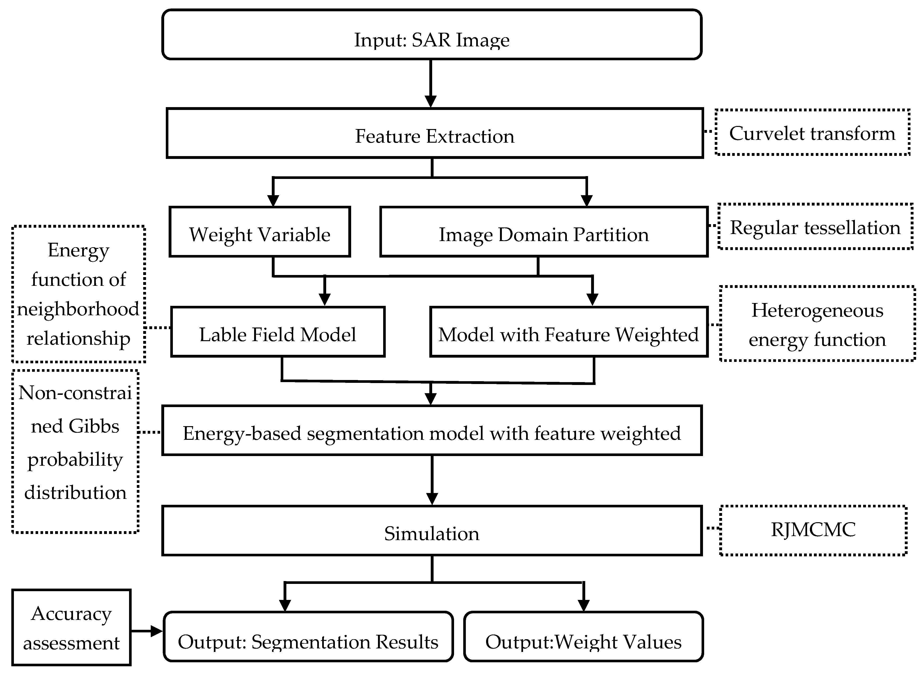
In summary, Figure 1 shows the flowchart of the proposed segmentation framework.

3. Results

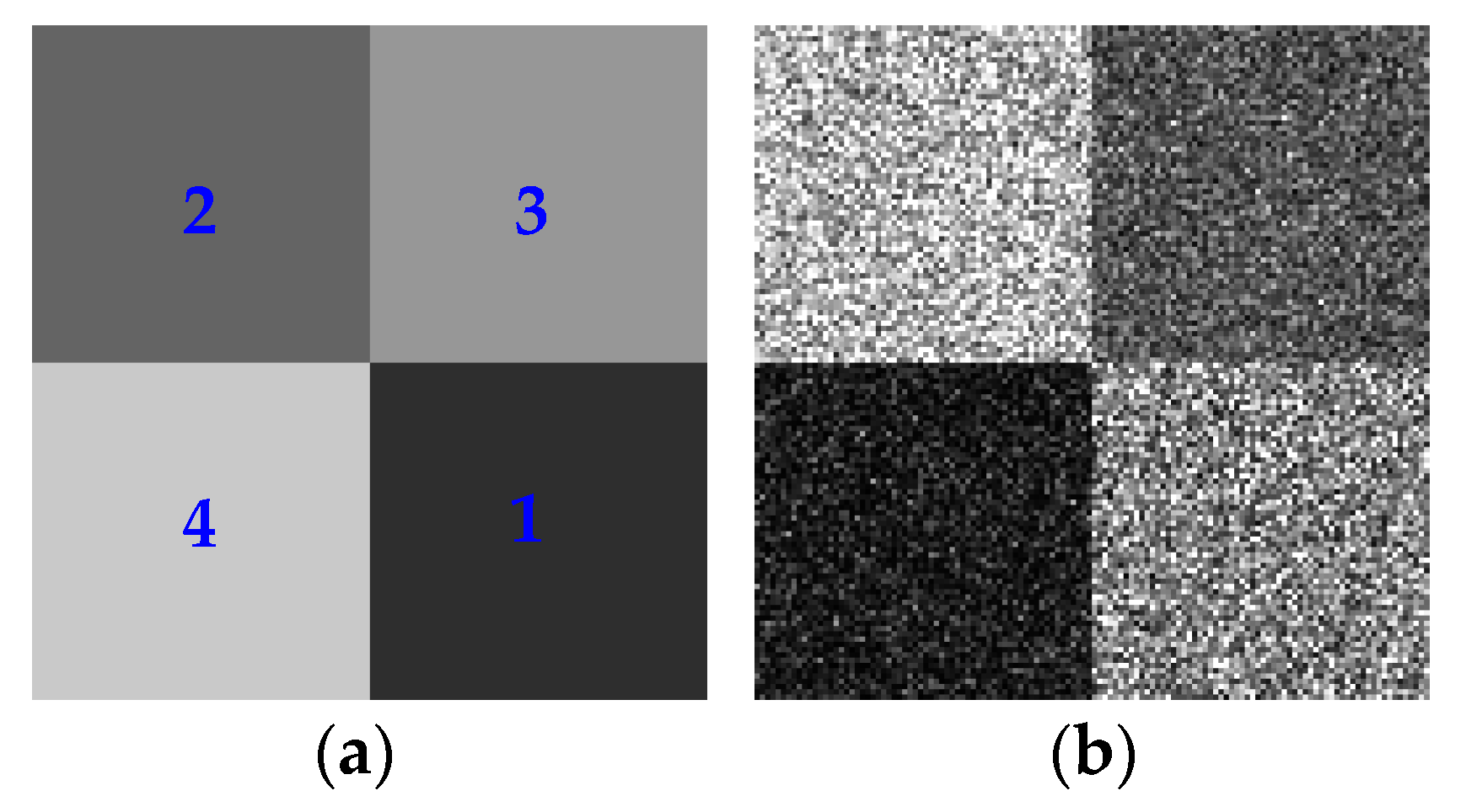
Given a multi-look SAR image in which the intensities of pixels are characterized by a Gamma distribution [24], α is equal to the number of its looks. In this paper, since α was considered as a random variable, the value µ_α was set as the number of looks. For Gamma distribution with parameters α and β, the product of the two parameters, α × β, was equal to its mean. Then the value µ_α × µ_β= E(α)E(β) = E(α × β) (the last equation is true, since α and β are independent, where E(·) is the mean operator) was taken as 128 = 256/2 (i.e., the midpoint of 256 grey levels) since the pixel intensities in a grey-scale image vary in the range of 0 and 255. Therefore, the shape parameter α and scale parameter β listed in

Table 1. Gamma parameters of a simulated SAR image.

Parameter	1	2	3	4
α	4.0664	7.6891	6.3832	2.2705
β	33.7712	24.1027	13.5704	48.3081

are assumed to respectively satisfy Gaussian distributions with means and standard deviations (μ_a, σ_α) and (μ_β, σ_β), where µ_α = 4, σ_α = 2, µ_β = 32 and σ_β = 24. Figure 2 shows an image temple and a simulated SAR image, where the simulated SAR image (see Figure 2b) is generated based on the image temple (shown in Figure 2a) and parameters listed in Table 1.

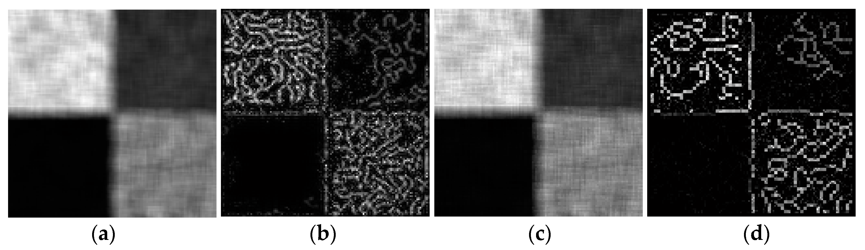
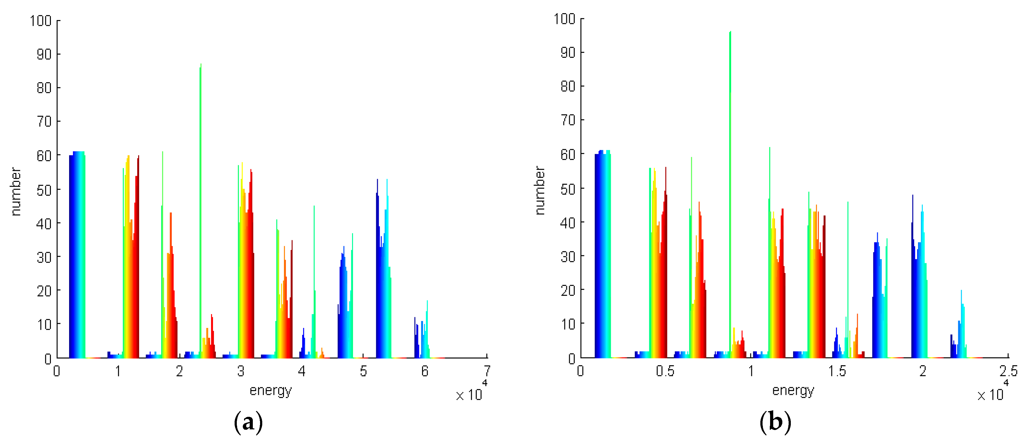
Figure 3a,b respectively show texture and boundary features extracted by using the curvelet transform. To verify the advantage of curvelet transform in extracting features, 2D harr wavelet transform is considered as a comparison algorithm to extract texture and boundary features using the same principle. These extraction results are shown in Figure 3c,d. Comparing with these texture features (see Figure 3a,c), it could be seen that they were very similar. To further compare with them, energy histograms of two transform are shown in Figure 4. From Figure 4, it could be seen that the shapes of the energy histograms distribution were similar, but the ranges of energy were different. The energy range of the curvelet transform was 0.25 × 10⁴–6 × 10⁴, and the energy range of the wavelet transform was 0.15 × 10⁴–2.25 × 10⁴. The larger the energy is, the more the image information is. Therefore, it can be found that curvelet texture feature contained more information, and curvelet transform could extract texture features more effectively. Comparing Figure 3b,d, it could be found that the boundary features extracted by the curvelet transform were more complete. From Figure 3 and Figure 4, it can be demonstrated that the information of the curvelet extracted features was more abundant and complete, and the curvelet transform could extract texture and boundary features better.

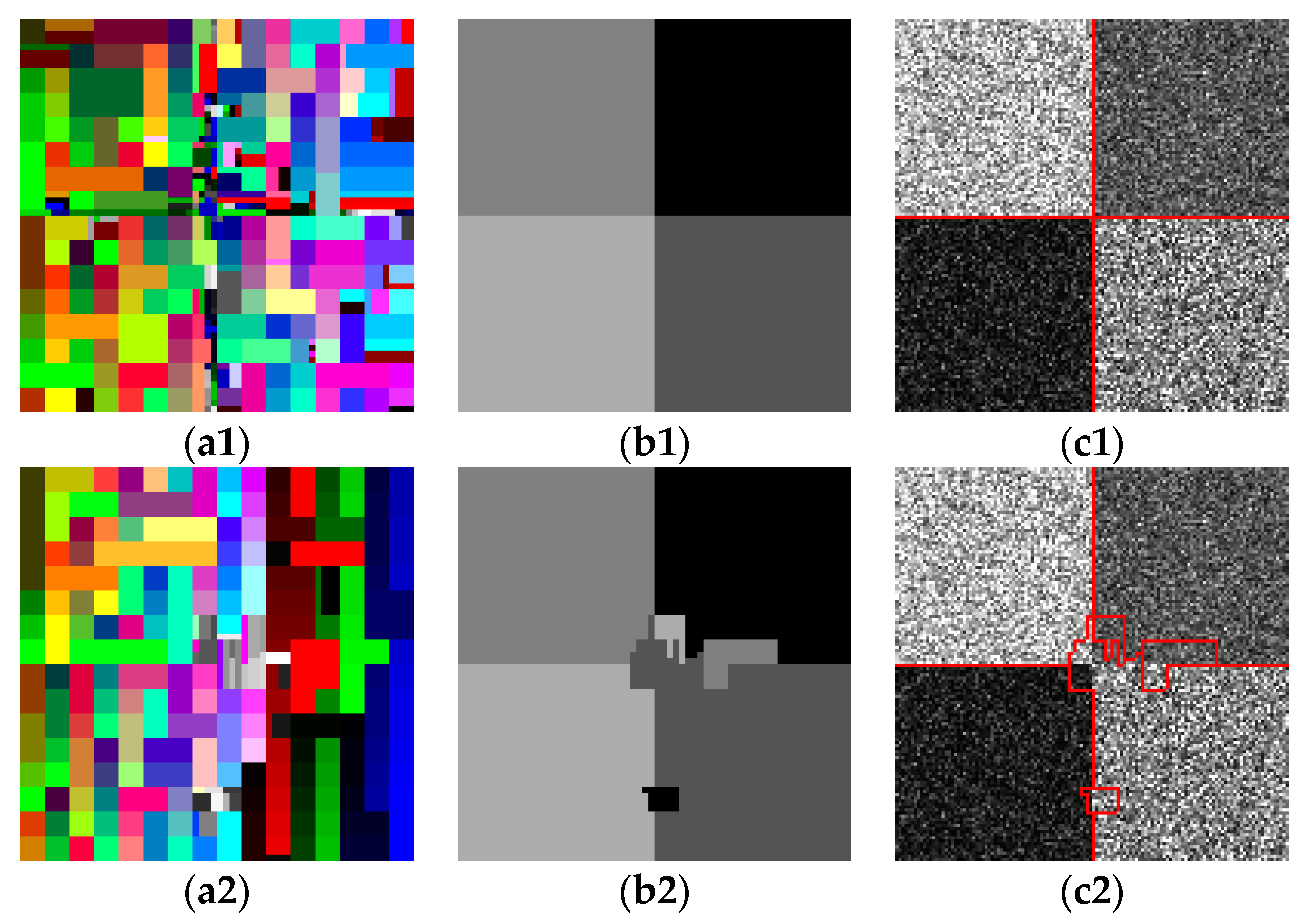
For the simulated SAR image, every pixel shows its intensity information. In this paper, the intensity information of a pixel is considered as its spectral feature, so the spectral features of all the pixels form the original spectral feature. The above extracted features and the original spectral feature form a curvelet feature set and wavelet feature set, respectively. The energy segmentation method with feature weighted was used to test on these feature sets, Figure 5a1–c1 show the visual evaluation results based on curvelet features, and Figure 5a2–c2 show the visual evaluation results by wavelet features. Figure 5a1,a2 are the results of regular tessellation, their every partitioned block is shown in a random color, and the colors of partitioned blocks in Figure 5a1 or a2 are different. Figure 5b1,b2 show the segmentation results. The outlines are extracted and overlaid on the original images, shown in Figure 5c1,c2. From Figure 5, it can be seen that there are some blocks crossing the boundaries in Figure 5b2, and the extracted outlines can not match the real boundaries precisely shown in Figure 5c2. Further, it could be illustrated that the proposed approach based on curvelet features could segment the simulated SAR image better.

To quantitatively evaluate the segmentation results of a simulated SAR image (see Figure 5b1,b2), their confusion matrixes, which are square arrays of numbers set out in rows and columns, which express the numbers of pixels assigned to a particular class in the segmentation results relative to the number of pixels assigned to a particular class in the reference image (see Figure 2a), were obtained, respectively. Then the producer’s accuracy, user’s accuracy, overall accuracy and Kappa coefficient can be computed as [25]:

$$\mathrm{Pr}{\mathrm{oducer}’\mathrm{s}\mathrm{accuracy}}_q=\frac{n_{qq}}{n_{+q}}$$

(21)

$${\mathrm{User}’\mathrm{s}\mathrm{accuracy}}_b=\frac{n_{oo}}{n_{o+}}$$

(22)

$${\mathrm{Overall}\mathrm{accuracy}}_q=\frac{{\displaystyle \sum _{o=1}^O{n}_{oo}}}{S}$$

(23)

$$\mathrm{Kappa}\mathrm{coefficient}=\frac{S{\displaystyle \sum _{o=1}^O{n}_{oo}}-{\displaystyle \sum _{o=1}^O{n}_{o+}{n}_{+o}}}{S^2-{\displaystyle \sum _{o=1}^O{n}_{o+}{n}_{+o}}}$$

(24)

where n_o+ is the sum of n_oq (q∈{1, …, O}); n_+q is the sum of n_oq (o∈{1, …, O}), denotes the number of pixels classified into class o in the segmentation result and class q in the reference image. The producer’s and user’s accuracies are used to determine individual class accuracies, overall accuracy and Kappa coefficient are used to determine the global class accuracy [25].

Table 2. Quantitative evaluation of a simulated SAR image.

Feature	Producer’s Accuracy (%)				User’s Accuracy (%)				Overall Accuracy (%)	Kappa Coefficient
	1	2	3	4	1	2	3	4
Curvelet	100	100	100	100	100	100	100	100	100	1.000
Wavelet	96.9	98.2	91.0	98.0	95.1	94.0	97.8	97.4	96.0	0.947

lists the quantitative evaluation of two segmentation results. From Table 2, it can be seen that all the segmentation accuracies of Figure 5b1 were 100%, and its Kappa coefficient was 1.000; the producer’s accuracy of 3 class and the user’s accuracy of 2 class were below 95.0%, and Kappa coefficient was 0.947 in the quantitative evaluation of Figure 5b2. Comparing with the results of two quantitative evaluations, it could be found that all the segmentation accuracies and Kappa coefficient of Figure 5b1 were higher. From the above quantitatively and qualitatively evaluation results, it could be demonstrated that the proposed method based on curvelet features could segment a simulated SAR image better.

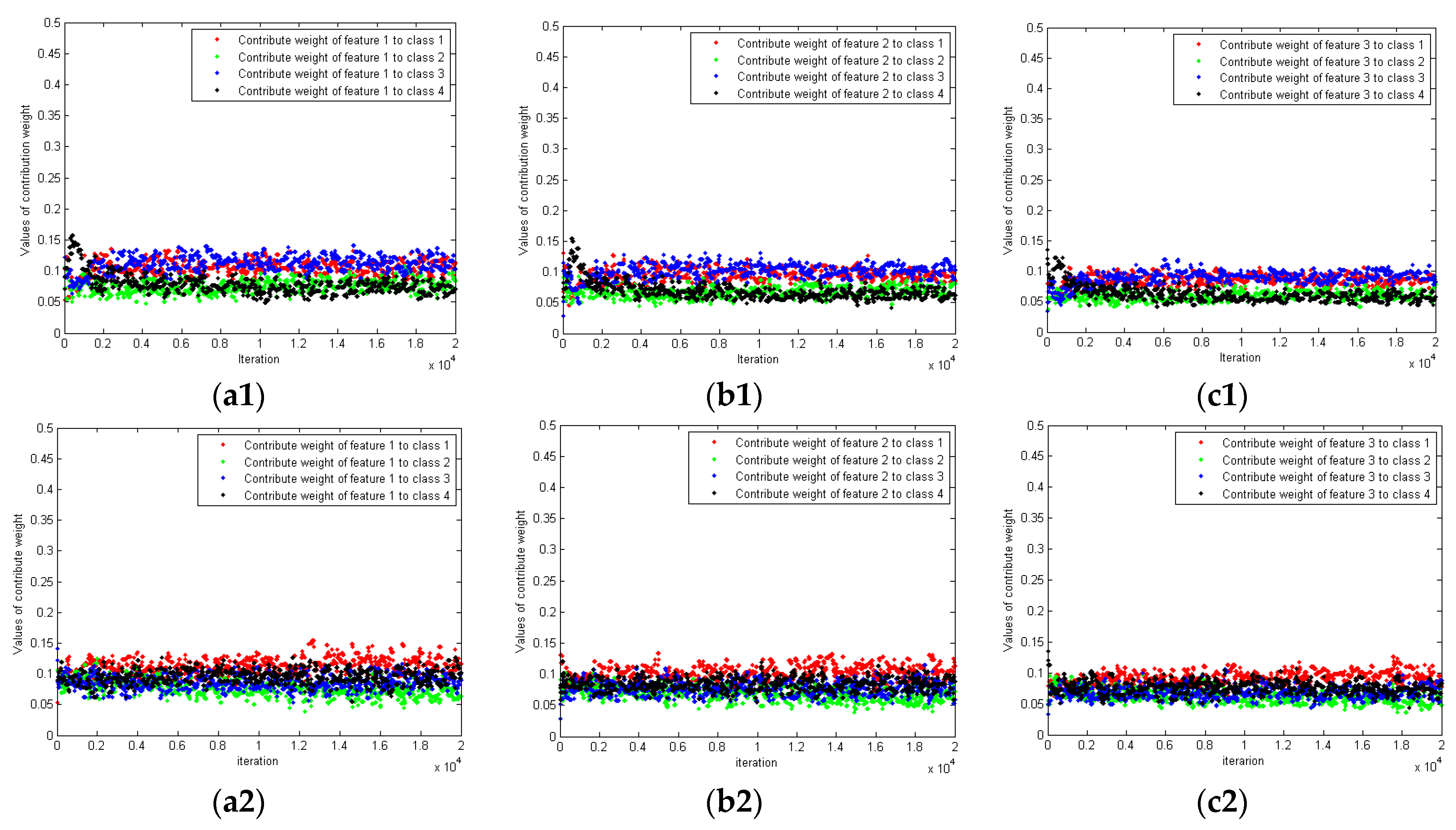
To explore the roles of multiple features in the segmentation procedure, weight variables of all the classes on the multiple features are defined. Their values are solved by the iteration processing. Figure 6 shows the changes of features’ weight values for all the classes, where Figure 6a1 and Figure 5a2 show the changes of spectral feature’s weight values for four classes, Figure 6b1,b2 show the changes of texture feature’s weight values for four classes and Figure 6c1,c2 show the change of boundary feature’s weight values of four classes. In Figure 6, a red point represents the weight value of features for class 1, a green point represents the weight value of every feature for class 2, a blue point represents the weight value of every feature for class 3 and a black point represents the weight value of every feature for class 4. From Figure 6, it can be seen that all the weight values quickly drive their approximate values listed in

Table 3. Approximate feature weight values for a simulated SAR image.

Feature	Spectral				Texture				Boundary
	1	2	3	4	1	2	3	4	1	2	3	4
Curvelet	0.12	0.07	0.12	0.06	0.10	0.06	0.11	0.05	0.10	0.06	0.10	0.05
Wavelet	0.12	0.06	0.08	0.10	0.11	0.05	0.08	0.09	0.11	0.05	0.07	0.08

. In Table 3, numbers 1–4 represent four classes of a simulated SAR image, and they correspond to numbers 1–4 shown in Figure 2b. The greater the weight value is, the more important the role of its feature is. Therefore, it could be demonstrated that the proposed method could automatically determine the roles of features in the segmentation procedure. From Table 3, it could be computed that the total weight values of three curvelet features were 0.37, 0.32 and 0.31, and the total weight values of three wavelet features were 0.36, 0.33 and 0.31. The greater total weight value of a feature, the more important its role is. Therefore, it could be found that the same rule that the role of spectral is the most important, and the role of boundary feature is the least important. However, their total weight values were slightly different, and these weight values of four classes for the same feature were slightly different. For example, two total weight values of spectral feature were 0.37 and 0.36, and their weight values of classes 2–4 were assigned differently. Another example, two total weight values of the boundary feature were the same, but their weight values of all the classes were different. The weight values can directly affect the segmentation results. It is known that the segmentation result by using the proposed method based on curvelet features is better. Therefore, it can be illustrated that the proposed method based on curvelet features can more reasonably assign the weights of all the class on the three features from Figure 3, Figure 4, Figure 5 and Figure 6 and Table 2 and Table 3.

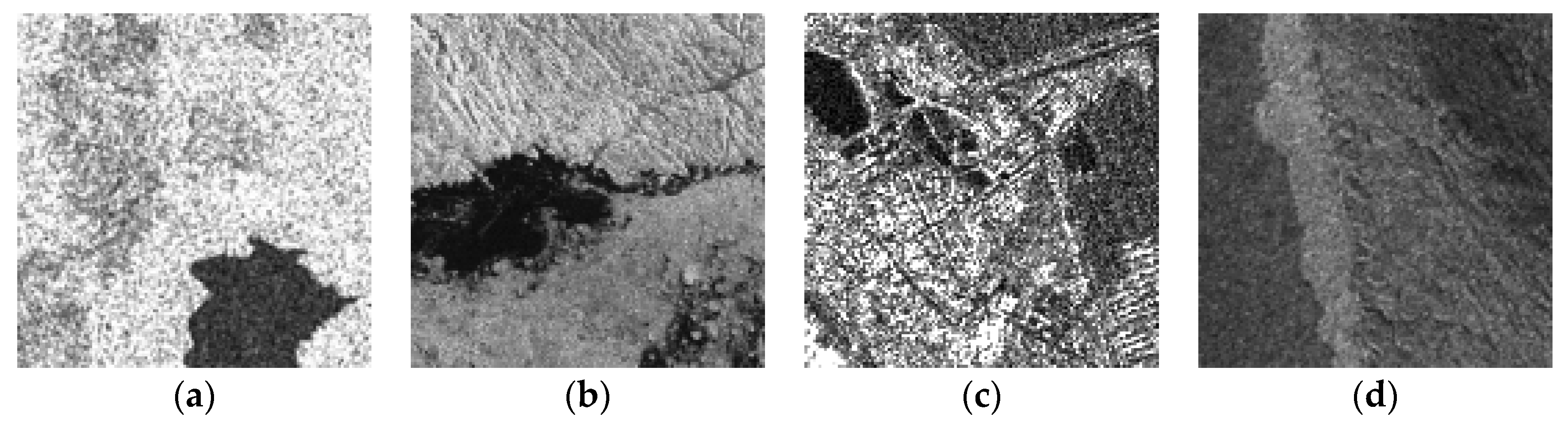
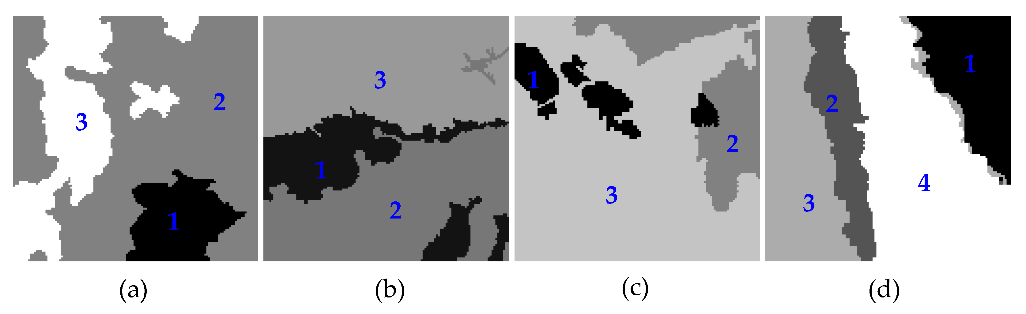
In summary, curvelet features are used in the segmentation tests of four RADARSAT-I/II images with 128 pixels × 128 pixels (shown in Figure 7). Figure 7a presents a RADARSAT-I image of a coastal scene with VV polarization and spatial resolution of 30 m, its scene is about 14.75 km², which reveals three types of sea ice structures, from bright to dark, respectively representing hard ice, melt ice and water; Figure 7b presents RADARSAT-II 4look image with HH polarization and spatial resolution of 25 m, the scene is 10.24 km², which reveals three types of areas, from bright to dark, respectively representing hard ice, melt ice and water; Figure 7c shows a RADARSAT-II image with HV polarization and spatial resolution of 25 m, its scene is 10.24 km², which reveals three types of areas, from bright to dark, respectively representing living area, field area and water area; Figure 7d presents a RADARSAT-I 4look image with VV polarization and spatial resolution of 50 m, the scene is 40.96 km², which reveals four types of sea ice structures (from left to right, representing melt ice, melt-hard ice, hard ice and an ice-water mixture) in Ungava Bay, Quebec, Canada.

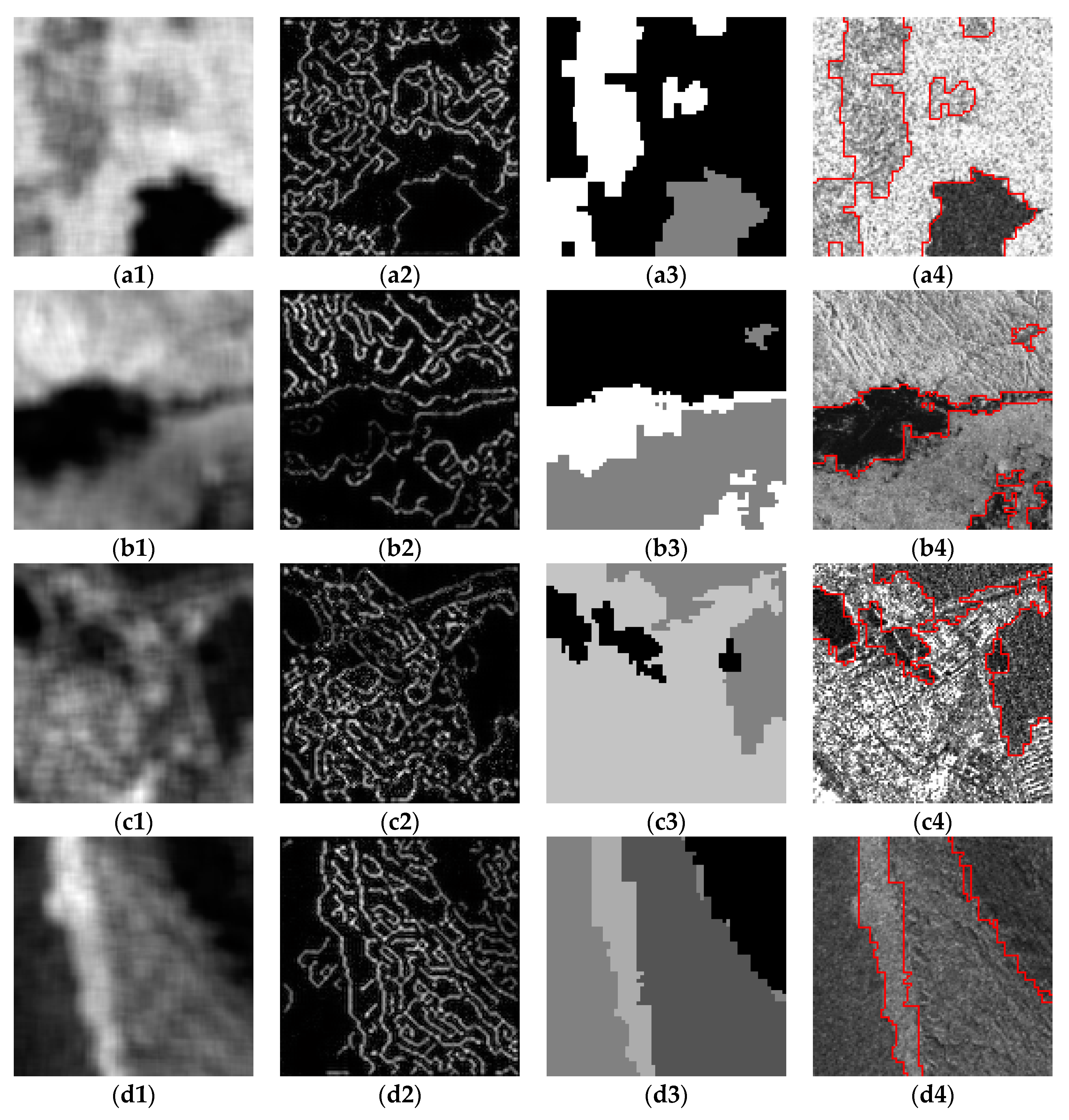
The proposed extraction methods are used to extract their texture and boundary features, Figure 8a1–d1 show texture features and Figure 8a2–d2 show boundary features. From them, it can be seen that the extracted boundary features were complete, and the extracted texture features were well. Further, it could be verified that curvelet transform could extract the texture and boundaries features of the real SAR images well. The extracted texture, boundary features and the original spectral feature form their own feature sets. The proposed method was tested on these feature sets of real SAR images. Figure 8a3–d3 show segmentation results, and their outlines were extracted to overlay on the original images, shown in Figure 8a4–d4. From Figure 8a4–d4, it can be seen that the extracted outlines match real boundaries of four real SAR images well. Further, it can be verified that the proposed method can segment four real SAR images well.

In order to assess the segmented results obtained by the proposed approach quantitatively, some common measures, including the producer’s accuracy, user’s accuracy, overall accuracy and Kappa coefficient, were computed by the temples of real SAR images (see Figure 9).

Table 4. Quantitative evaluation of a simulated SAR image.

Image	Producer’s Accuracy (%)				User’s Accuracy (%)				Overall Accuracy (%)	Kappa Coefficient
	1	2	3	4	1	2	3	4
7(a)	95.3	96.3	94.2		96.1	96.8	92.9		95.7	0.918
7(b)	91.7	94.4	98.0		87.3	95.9	98.8		95.4	0.928
7(c)	94.1	98.5	96.0		87.2	89.9	99.3		96.3	0.916
7(d)	97.7	86.5	95.5	98.0	93.9	95.5	96.3	98.6	96.1	0.938

lists them. From Table 4, it can be seen that only four accuracies were below 91.7%, overall accuracies were up to 95.0% and Kappa coefficients were higher than or equal to 0.916. Further, it could be demonstrated that the proposed method was feasible and effective.

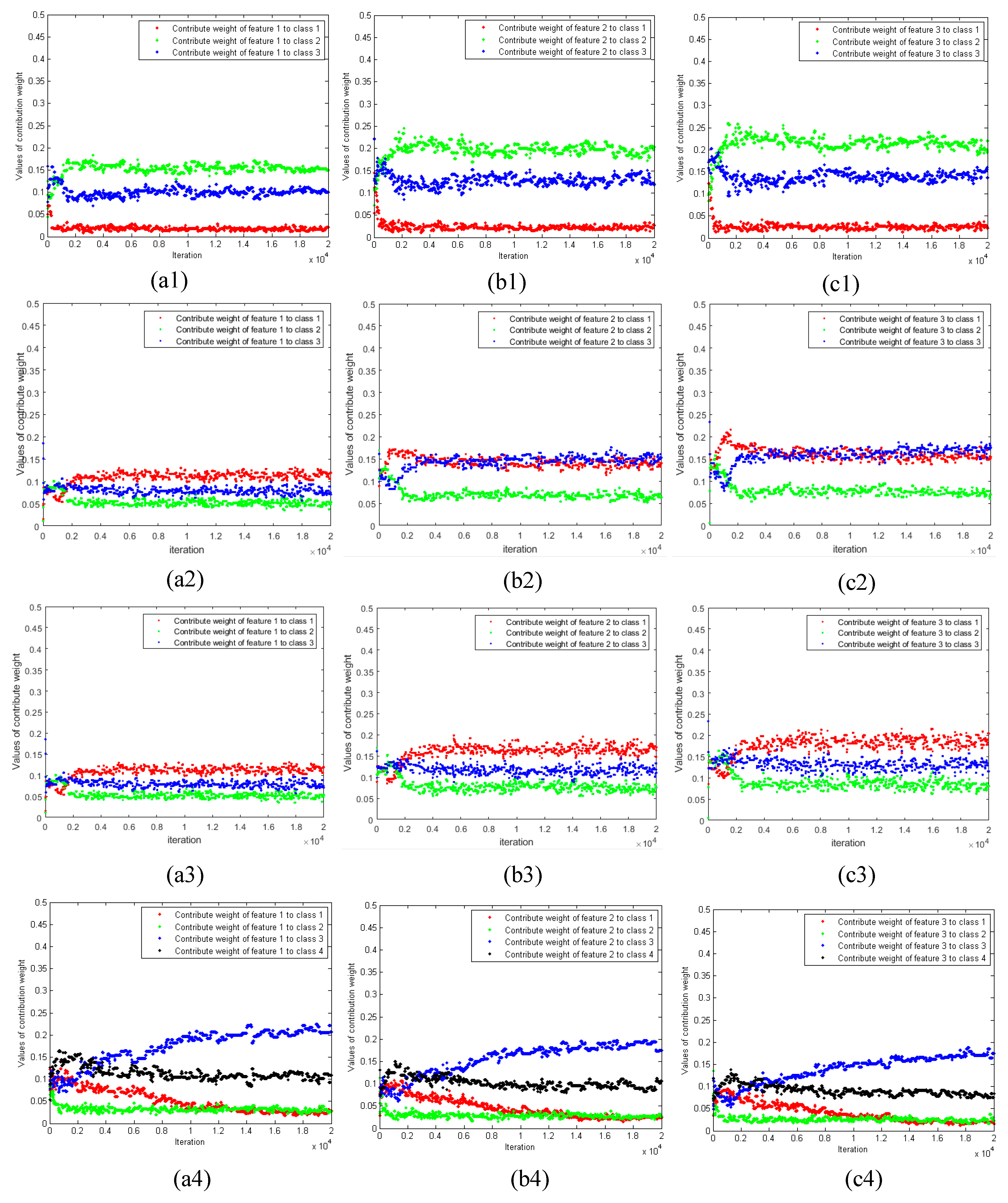
Figure 10 shows the changes of features’ weight values for all the classes in real SAR images, where Figure 10a1–a4 show the changes of spectral feature’s weight values for all the classes, Figure 10b1–b4 show the changes of texture feature’s weight values for all the classes and Figure 10c1–c4 show the change of boundary feature’s weight values for all the classes. In Figure 10, a red point represents the weight value of every feature for class 1, a green point represents the weight value of every feature for class 2, a blue point represents the weight value of every feature for class 3 and a black point represents the weight value of every feature for class 4. From Figure 10, it can be seen that the weight values quickly drive their approximate values listed in

Table 5. Approximate feature weight values for real SAR images.

Images	Spectral				Texture				Boundary
	1	2	3	4	1	2	3	4	1	2	3	4
6(a)	0.01	0.16	0.11		0.01	0.22	0.13		0.01	0.22	0.13
6(b)	0.12	0.05	0.08		0.14	0.07	0.15		0.15	0.07	0.17
6(c)	0.12	0.05	0.07		0.17	0.08	0.11		0.20	0.08	0.12
6(d)	0.02	0.03	0.11	0.20	0.02	0.03	0.10	0.19	0.02	0.03	0.08	0.17

. From Table 5, it can be computed that the total weight values of Figure 7a‘s three features were 0.28, 0.36 and 0.36; the total weight values of Figure 7b‘s three features were 0.25, 0.36 and 0.39; the total weight values of Figure 7c’s three features were 0.24, 0.36 and 0.40 and the total weight values of Figure 7d’s three features were 0.36, 0.34 and 0.30. Therefore, it can be found that the role of Figure 7a’s texture and boundary features were same, and the role of its spectral feature was the least important; the role of Figure 7b’s boundary was the most important, and the role of its spectral feature was the least important; and the role of Figure 7c’s boundary feature was the most important, and the role of its spectral feature was the least important; and the role of Figure 7d’s spectral feature was the most important, and the role of its boundary feature was the least important. From Figure 8 and Figure 10 and Table 4 and Table 5, it can be illustrated that the proposed method can not only explore the roles of multiple features in the segmentation procedure, but also segment the real SAR images well.

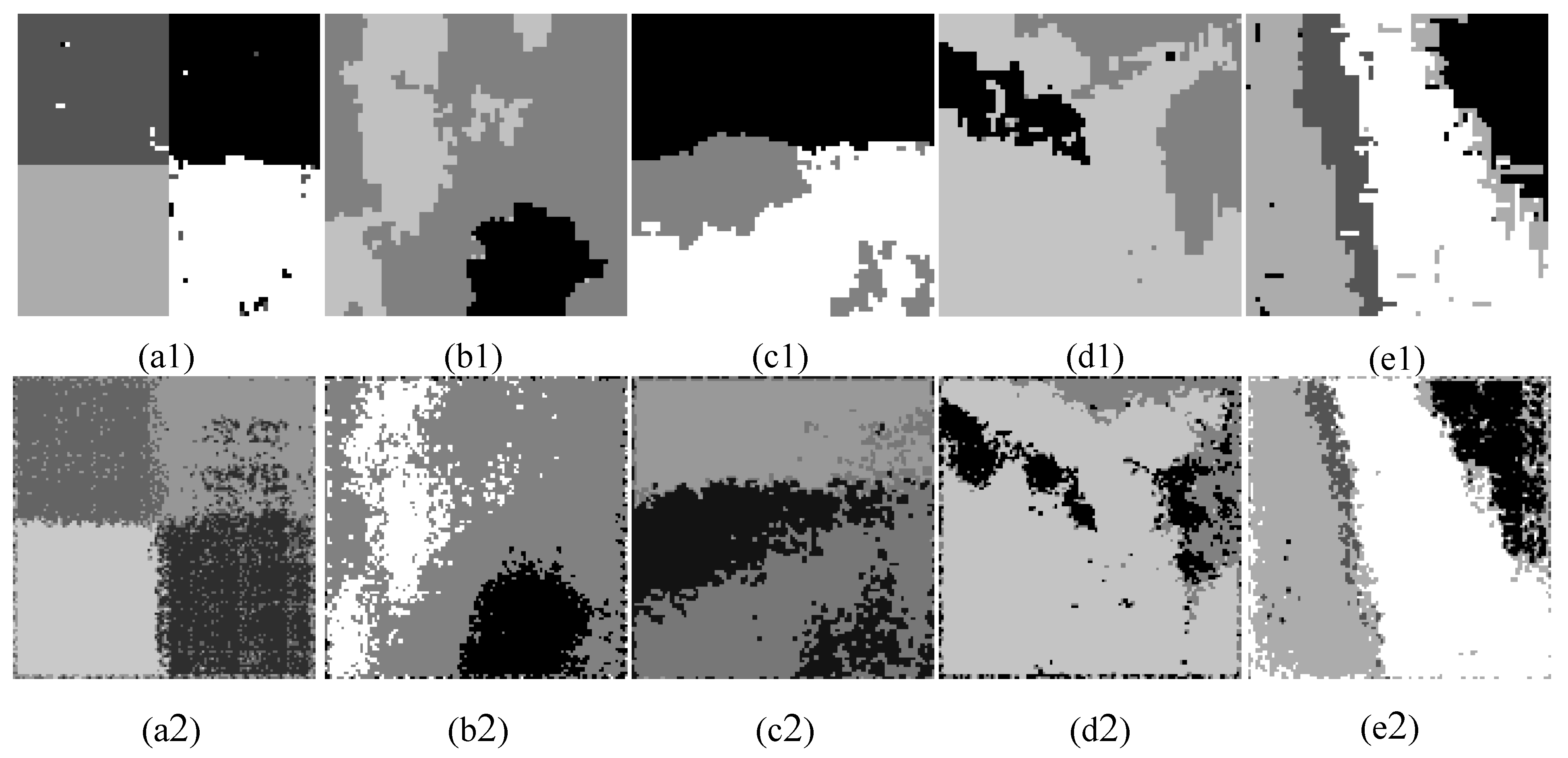
To illustrate the advantage of the proposed method, two methods were chosen as comparison methods. Method 1 was the proposed method without weight. In this method, the roles of the three same features (spectral, texture and boundary features) were the same in the segmentation procedure, it may reduce the segmentation accuracy, because of feature redundancy. Another method was a VGG16 net-based fully convolutional network (FCN) [26]. The method changes the full connection layer of VGG16 net to a full convolution layer, and incorporates multilayer high and low dimensional feature information; but this method is a pixel-based method, it does not consider the relations among pixels. Figure 11 shows the segmentation results of the comparison of methods, Figure 11a1–e1 are the segmentation results by using the proposed method without weight, Figure 11a2–e2 are the segmentation results by using FCNs. From Figure 11a1–e1, it can be seen that some incorrect segmentation pixels existed in the homogeneous regions and crossing the boundaries. In particular, the phenomenon existed in Figure 11a1,e1. Comparing the segmentation results of the proposed method and the segmentation results of the proposed method without weight, it could be seen that the proposed method could segment the SAR image better.

Table 5 illustrated that the proposed method, which researches on the roles of features in the segmentation procedure, could improve the segmentation results. From Figure 11a2–e2, it can be seen that the boundaries between regions and outer boundaries of images were very blurry. For example, the segmented boundaries between regions in Figure 11a2 were very blurry, and the outer boundaries shown in Figure 11d2,e2 were blurry. In addition, incorrect segmentation pixels existed in the regions, especially in the right of Figure 11a2, the phenomenon was very obvious. Further, it can be illustrated that the segmentation results of FCN may be influenced by the speckle noise of the SAR image, as it is a pixel-based method. Comparing with these segmentation results, it can be seen that the proposed method’s segmentation results were better. Further, the superiority of the proposed method could be demonstrated.

To further demonstrate the advantage of the proposed method, the segmentation results of the comparison methods were evaluated quantitatively.

Table 6. Quantitative evaluation of the comparison of methods.

Method	Image	Producer’s Accuracy(%)				User’s Accuracy(%)				Overall Accuracy(%)	Kappa Coefficient
		1	2	3	4	1	2	3	4
Method 1	2(b)	95.9	97.1	97.1	100	95.8	97.5	96.8	100	97.5	0.966
	7(a)	95.5	93.7	92.8		93.2	96.2	88.2		93.7	0.882
	7(b)	85.0	90.7	98.0		84.2	91.4	97.8		92.8	0.886
	7(c)	84.2	97.7	93.6		74.3	84.1	99.1		93.6	0.857
	7(d)	92.8	89.0	97.2	91.4	95.0	94.2	84.3	98.3	92.9	0.898
Method 2	2(b)	77.9	85.0	75.1	90.8	84.9	72.1	78.0	96.6	82.2	0.763
	7(a)	91.3	88.2	63.9		75.4	84.7	79.8		82.4	0.661
	7(b)	81.3	80.1	70.2		51.9	76.6	98.2		76.1	0.637
	7(c)	68.4	58.6	90.7		42.3	72.2	92.6		82.9	0.608
	7(d)	64.9	25.6	87.9	96.3	96.8	60.2	65.5	87.6	79.0	0.690

lists their producer’s accuracies, user’s accuracies, overall accuracies and Kappa coefficients. Comparing with the quantitative results of the proposed method and comparison methods, it could be obviously found that the overall accuracies and Kappa coefficients of the proposed method were higher.

4. Discussion

In this paper, a feature weighted SAR image segmentation method based on energy function is presented.

In exploring the law of all the features’ roles in the segmentation procedure, a series of experiments were conducted (see Figure 6 and Figure 9). From them, it could be found that the weight values quickly drove their approximate values and remained unchanged during the iteration processing. Furthermore, it could be proved that the proposed approach could automatically determine the roles of all the features in the segmentation procedure.

From Figure 5 and Figure 8, it can be found that the proposed approach could segment a simulated and a real SAR image well, especially a simulated SAR, its segmentation result did not have existing incorrect segmentation blocks. From Figure 3 and Figure 4, it could be found that the image information of the extracted features by using the curvelet transform was more abundant and complete, and then the advantage of the curvelet transform in feature extraction could be demonstrated. According to the comparison with the segmentation results of a simulated SAR image by using the proposed approach based on curvelet and wavelet features, it could be found that the more image information the feature contains, the better the segmentation result will be. It could be proved that the extracted features could affect the segmentation results. Comparing Figure 5, Figure 8 and Figure 11, it can be found that the proposed method could segment SAR images better. Further, it could be demonstrated the superiority of the proposed method.

5. Conclusions

To extract more structural features that can contribute to segmenting a SAR image accurately, and explore the roles of the features in the segmentation procedure, this paper proposed a block- and energy-based segmentation method with feature weighted for the SAR image. In this paper, the curvelet transform was used to construct boundary and texture features, and they were incorporated into the statistical segmentation models in a weighted way, that is, an energy segmentation model with a weighted feature. The proposed method was tested on simulated and real SAR images, the results showed that the proposed method could not only automatically determine the roles of all the features in the segmentation procedure, but also segment SAR images well. This method needs to give the number of classes a priori. For a SAR image, it is difficult to artificially determine the number of classes. The difficulty drives from the speckle noise of a SAR image. In future work, the unknown number of classes in a SAR image will be assumed as a variable, and a move of sampling the number of the classes can be designed to solve its value in the RJMCMC algorithm.

References

- Jensen, J.R. Introductory Digital Image Processing: A Remote Sensing Perspective, 3rd ed.; Prentice Hall: Upper Saddle River, NJ, USA, 2006. [Google Scholar]
- Richards, J.A.; Jia, X. Remote Sensing Digital Image Analysis: An Introduction, 4th ed.; Springer: Berlin, Germany, 2006. [Google Scholar]
- Cao, Y.F.; Sun, H.; Xu, X. An unsupervised segmentation method based on MPM for SAR images. IEEE Geosci. Remote Sens. Lett. 2005, 2, 55–58. [Google Scholar] [CrossRef]
- Zhang, J.T.; Zhang, L.M. A watershed algorithm combining spectral and texture information for high resolution remote sensing image segmentation. Geomat. Inf. Sci.Wuhan Univer. 2017, 42, 449–455. [Google Scholar]
- Acqua, D.F.; Gamba, P.; Ferrariet, A.; Palmason, J.A.; Benediktsson, J.A.; Arnason, K. Exploiting spectral and spatial information in hyperspectral urban data with high resolution. IEEE Geosci. Remote Sens. Lett. 2004, 1, 322–326. [Google Scholar] [CrossRef]
- Chen, Y.X.; Qin, K.; Gan, S.Z.; Wu, T. Structural feature modeling of high resolution remote sensing images using directional spatial correlation. IEEE Geosci. Remote Sens. Lett. 2014, 11, 1727–1731. [Google Scholar] [CrossRef]
- Xue, X.R.; Wang, H.F.; Xiang, F.; Wang, J.P. A new method of SAR image segmentation based on FCM and wavelet transform. In Proceedings of the 2012 5th International Congress on Image and Signal Processing, Chongqing, China, 16–18 October 2012. [Google Scholar]
- Dey, S.; Goswami, R.S. A morphological segmentation and curvelet features extraction on text region classification using SVM. In Proceedings of the 2015 IEEE International Conference on Computational Intelligence and Computing Research (ICCIC), Madurai, India, 10–12 December 2015. [Google Scholar]
- Rahmani, M.; Akbarizadeh, G. Unsupervised feature learning based on sparse coding and spectral clustering for segmentation of synthetic aperture radar images. IET Comput. Vis. 2015, 9, 629–638. [Google Scholar] [CrossRef]
- Liu, Z.; Fan, X.W.; Lv, F.Y. SAR Image Segmentation using contourlet and Support Vector Machine. In Proceedings of the 2009 Fifth International Conference on Natural Computation, Tianjin, China, 14–16 August 2009. [Google Scholar]
- Wang, M.; Zhou, S.D.; Bai, H.; Ma, N.; Ye, S. SAR water image segmentation based on GLCM and wavelet textures. In Proceedings of the 2010 6th International Conference on Wireless Communications Networking and Mobile Computing (WiCOM), Chengdu, China, 23–25 September 2010. [Google Scholar]
- Hao, B.; Zhang, X.R.; Li, N. MPM SAR Image Segmentation Using Feature Extraction and Context Model. IEEE Geosci. Remote Sens. Lett. 2012, 9, 1041–1045. [Google Scholar]
- Lv, N.; Chen, C.; Qiu, T.; Sangaiah, A.K. Deep learning and superpixel feature extraction based on Contractive Autoencoder for change detection in SAR images. IEEE Trans. Ind. Inform. 2018, 14, 5530–5538. [Google Scholar] [CrossRef]
- Zhao, Q.H.; Li, Y.; Liu, Z.G. SAR image segmentation using Voronoi tessellation and Bayesian inference applied to dark spot feature extraction. Sensors 2013, 13, 14484–14499. [Google Scholar] [CrossRef] [PubMed]
- Chen, Y.H.; Zhu, L.; Yuille, A.; Zhang, H.J. Unsupervised learning of Probabilistic Object Models (POMs) for object classification, segmentation, and recognition using knowledge propagation. IEEE Trans. Pattern Anal. 2009, 31, 1747–1761. [Google Scholar] [CrossRef] [PubMed]
- Wu, Y.H.; Ji, K.F.; Yu, W.X.; Su, Y. Region-based classification of Polarimetric SAR images using Wishart MRF. IEEE Geosci. Remote Sens. Lett. 2008, 5, 668–672. [Google Scholar] [CrossRef]
- Candes, E.; Demanet, L.; Donoho, D.; Ying, L.X. Fast discrete curvelet transform. Multiscale Model. Sim. 2006, 5, 861–899. [Google Scholar] [CrossRef]
- Rahulkar, A.D.; Jadhav, D.V.; Holambe, R.S. Fast discrete curvelet transform based anisotropic feature extraction for IRIS recognition. ICTACT J. Image Video Process 2010, 11, 69–75. [Google Scholar] [CrossRef]
- Zhang, Y.; Rockett, P.I. The Bayesian operating point of the Canny edge detector. IEEE Trans. Image Process. 2006, 15, 3409–3416. [Google Scholar] [CrossRef]
- Duan, Y.P.; Liu, F.; Jiao, L.C. Skecching model and higher order neighborhood markov random field-based SAR image segmentation. IEEE Geosci. Remote Sens. Lett. 2016, 13, 1686–1690. [Google Scholar] [CrossRef]
- Kervrrann, C.; Heitz, F. A markov random field model-based approach to unsupervised texture segmentation using local and global spatial statistics. IEEE Trans. Image Process. 1995, 4, 856–862. [Google Scholar] [CrossRef] [PubMed]
- Zhao, Q.H.; Zhang, H.Y.; Li, Y. Regionalized image segmentation using Kolmogorov-Smirnov statistics. J. Image Graph. 2015, 20, 678–686. [Google Scholar]
- Green, P.J. Reversible jump markov chain monte carlo computation and Bayesian model determination. Biometrika 1995, 82, 711–732. [Google Scholar] [CrossRef]
- Li, Y.; Li, J.; Chapman, M.A. Segmentation of SAR intensity imagery with a Voronoi tessellation, Bayesian inference, and Reversible Jump MCMC algorithm. IEEE Trans. Geosci. Remote Sens. 2010, 48, 1872–1881. [Google Scholar] [CrossRef]
- Congalton, R.G.; Green, K. Assessing the Accuracy of Remotely Sensed Data: Principles and Practices; CRC Press: Boca Raton, FL, USA, 2008. [Google Scholar]
- Long, J.; Shelhamer, E.; Darrell, T. Fully Convolutional Networks for semantic segmentation. IEEE T Pattern Anal. 2014, 39, 640–651. [Google Scholar]
Figure 1.
Flowchart of the proposed segmentation framework.
Figure 2.
Temple and simulated synthetic aperture radar (SAR) images: (a) Temple image, (b) simulated SAR image.
Figure 3.
Texture and boundary features of a simulated SAR image: (a) Texture feature by using the curvelet transform, (b) boundary feature by using the curvelet transform, (c) texture feature by using the wavelet transform, (d) boundary feature by using the wavelet transform.
Figure 4.
Energy histograms of a simulated SAR image: (a) Curvelet, (b) wavelet.
Figure 5.
Visual evaluation results of a simulated SAR image: (a1,a2) Regular tessellation, (b1,b2) segmentation result, (c1,c2) extracted outlines on the original image.
Figure 6.
Changes of features’ weight values for all the classes by using curvelet and wavelet feature sets: (a1,a2) Feature 1, (b1,b2) feature 2, (c1,c2) feature 3.
Figure 7.
Four real SAR images (a–d).
Figure 8.
Results of real SAR images: (a1–d1) Texture features, (a2–d2) boundary features, (a3–d3) segmentation results, (a4–d4) overlaying the extracted outlines on the original images.
Figure 9.
Temples of real SAR images: (a–d) Temple images.
Figure 10.
Changes of features’ weight values for all the classes: (a1–a4) Feature 1, (b1–b4) feature 2, (c1–c4) feature 3.
Figure 11.
Segmentation results of comparison methods: (a1–e1) The proposed method without weight, (a2–e2) FCN-based method.