Mapping Mangrove Extent and Change: A Globally Applicable Approach

Abstract

This study demonstrates a globally applicable method for monitoring mangrove forest extent at high spatial resolution. A 2010 mangrove baseline was classified for 16 study areas using a combination of ALOS PALSAR and Landsat composite imagery within a random forests classifier. A novel map-to-image change method was used to detect annual and decadal changes in extent using ALOS PALSAR/JERS-1 imagery. The map-to-image method presented makes fewer assumptions of the data than existing methods, is less sensitive to variation between scenes due to environmental factors (e.g., tide or soil moisture) and is able to automatically identify a change threshold. Change maps were derived from the 2010 baseline to 1996 using JERS-1 SAR and to 2007, 2008 and 2009 using ALOS PALSAR. This study demonstrated results for 16 known hotspots of mangrove change distributed globally, with a total mangrove area of 2,529,760 ha. The method was demonstrated to have accuracies consistently in excess of 90% (overall accuracy: 92.2–93.3%, kappa: 0.86) for mapping baseline extent. The accuracies of the change maps were more variable and were dependent upon the time period between images and number of change features. Total change from 1996 to 2010 was 204,850 ha (127,990 ha gain, 76,860 ha loss), with the highest gains observed in French Guiana (15,570 ha) and the highest losses observed in East Kalimantan, Indonesia (23,003 ha). Changes in mangrove extent were the consequence of both natural and anthropogenic drivers, yielding net increases or decreases in extent dependent upon the study site. These updated maps are of importance to the mangrove research community, particularly as the continual updating of the baseline with currently available and anticipated spaceborne sensors. It is recommended that mangrove baselines are updated on at least a 5-year interval to suit the requirements of policy makers.

1. Introduction

Mangrove forests are tropical woody vegetation located along tropical coastlines in 118 countries and territories [1]. They are at the interface between the land and ocean and provide a range of ecosystem services at local through to the global scale. Mangroves are among Earth’s most highly productive aquatic ecosystems with a primary productivity of 2.5 g C m⁻² day⁻¹ [2], despite occupying regularly inundated saline environments where anoxic conditions are inhibitive to growth to most terrestrial species. Recent studies have shown that mangroves can store up to an average 1023 Mg C ha⁻¹ [3], sequestering up to four times as much carbon as terrestrial tropical forests [4]. Globally, mangrove forests store 4.19 Pg of Carbon within their vegetation and first 1 m of soils [5]. As a result mangrove forests have the potential to play an important role within carbon accrediting and Payment for Ecosystem Services (PES) schemes [6].

Mangrove forests also harbor a wide range of biodiversity as they straddle the terrestrial and aquatic biomes. They are an important habitat for a range of aquatic [7,8,9,10] and terrestrial species [11,12,13], including niche species such as the Royal Bengal Tiger [14]. Mangrove forests also have a socio-economic importance for local populations, ranging from the provision of construction materials and fuel [15,16,17] to a range of indirect products and services such as protection from storm surges and maintaining water quality [18,19,20,21]. In total, the economic benefits of mangrove forests are estimated at US $30.50 ha⁻¹ yr⁻¹ [22,23]. Knowledge on the status of mangrove forests is of critical importance for their conservation and the provision of the ecosystem services that they provide.

Despite their importance, mangrove forests are threatened across their entire range. Their extent is estimated to have decreased by 3.6 million ha between 1980 and 2005 [24] at a rate of up to 0.39% yr⁻¹ over 2000–2012 [25]. An estimated one third of mangrove forest has been lost over the past half-century [26]. The largest driver of this loss has been the conversion of mangrove forest to aquaculture [27], the fastest growing animal-food sector in the world [28]. This activity has been the most frequent cause of land cover change in mangrove forests over the period 1996–2010, particularly in Southeast Asia where two thirds of mangrove forest is located [29,30]. Knowledge on the status of mangrove forests is therefore of critical importance yet the mapped data products required to achieve this are not currently available on a regular basis and are difficult to repeat on an annual basis.

Most studies of mangrove forest extent have focused upon specific regions [31,32]. These use methods that are optimized to a specific study site, sometimes using local ancillary datasets, that may not be applicable to continental nor global scales. Attempts to make global scale assessments of mangrove extent have consolidated numerous national or regional scale inventories with varying degrees of precision and accuracy [24,33,34] due to differences in the time-period and methods used for adjacent maps [35,36,37]. Data from remote sensing satellites offers the potential for mapping mangrove extent over large areas using standardized approaches with a quantifiable assessment of accuracy. The first global map of mangrove forests that utilized remotely sensed data was the map of Giri et al. [1]. This work used over 1000 Landsat scenes acquired over the period 1997–2000, estimating a total mangrove extent of 13,776,000 ha. Although successful in determining a global extent map, this approach is limited in its ability to provide an operational monitoring system through successive annual baselines, due to attenuation of optical data by cloud cover and atmospheric conditions. Furthermore, single studies like these provide snapshots in time with no coherent method of updating the baseline, quickly rendering the dataset outdated in regions of rapid change.

Existing mangrove maps [1,33] have provided valuable estimates of global mangrove extent but they do not represent viable approaches for the routine monitoring of changes in extent over time. More recently, the CGMFC-21 (Global Database of Continuous Mangrove Forest Cover for the 21st Century) study [25] quantified changes in extent and carbon stocks using the intersection of a mangrove baseline [1], mangrove biome extent [38] and global forest change for 2000 to 2012 [39], thereby estimating global mangrove change. This represented the first study to estimate global mangrove change in a consistent and repeatable manner using a single methodology but was limited in terms of its ability to detect changes outside of established mangrove extent and outside of the Global Forest Cover definition of forests due to its reliance on existing datasets. This dependence limits the monitoring of mangroves despite the continued provision of remotely sensed data, due to its reliance on data products rather than raw data.

Synthetic Aperture Radar (SAR) data is not affected by cloud conditions and has been used to map mangrove extent and change [29] but has yet to be used for monitoring mangrove extent over very large regions, particularly at the global scale. This is despite cloud free global radar data being available from 1996 (JERS-1) to the present day (ALOS-2 PALSAR-2, Sentinel-1). The aim of this paper is to present a new approach for mapping and monitoring mangrove extent, that is repeatable, globally applicable, automated and specifically focused on mangroves. This is achieved by creating a new mangrove baseline from globally available datasets and implementing a novel map-to-image change detection technique to JERS-1 and ALOS PALSAR SAR imagery. The approach, which forms the basis of the methodology used for global mangrove monitoring within the Global Mangrove Watch project [40], is demonstrated using 16 sites located across the global extent of mangroves.

2. Study Sites

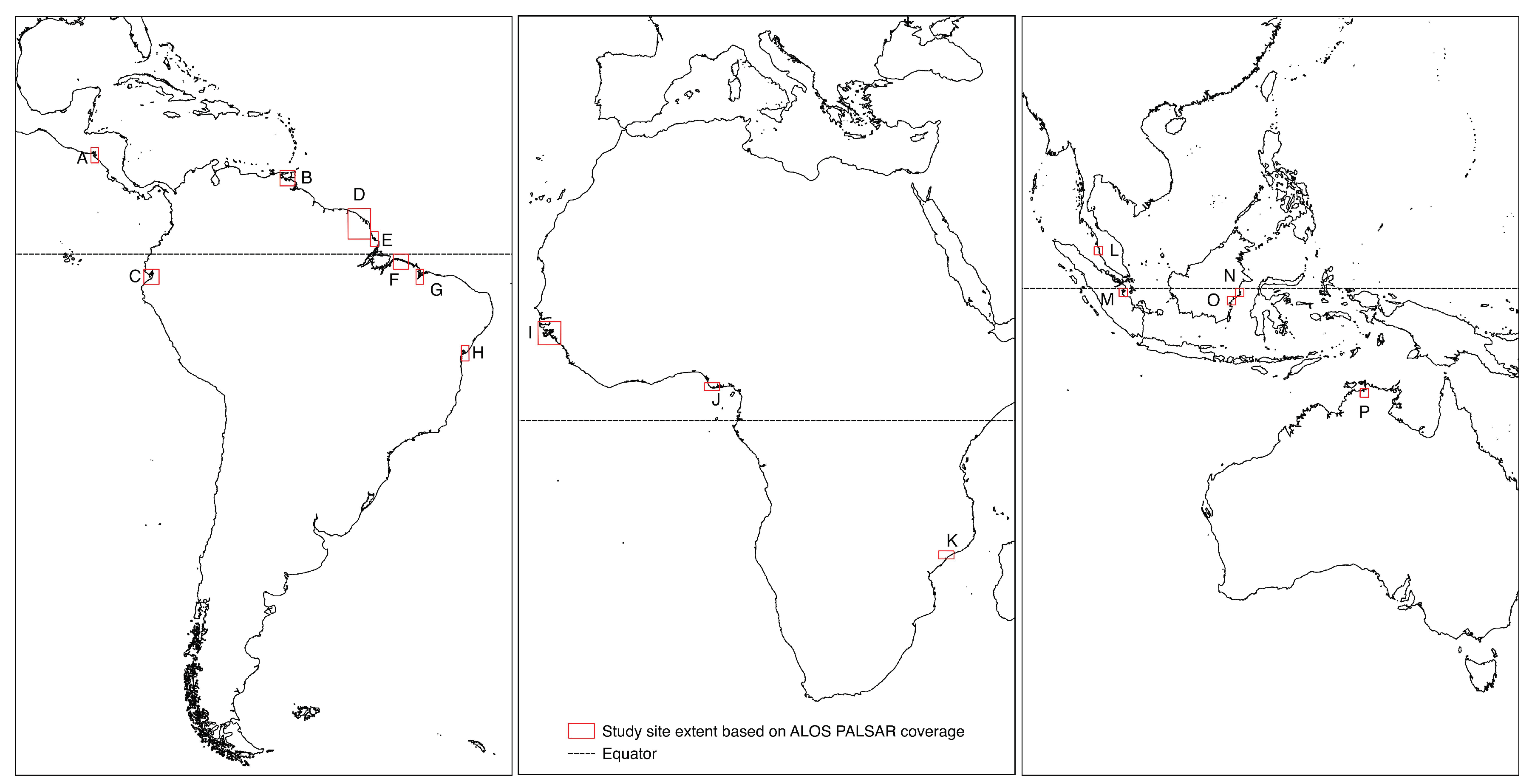
The novel approach for mapping and monitoring mangrove extent was developed and tested using 16 study areas representing the global range of mangrove forests (

Table 1. Selection criteria for study sites, based on a range of different mangrove environments, composition and characteristics. Two study sites were processed separately at East Kalimantan but are presented together in the table due to their similarity.

Study Site	Surrounding Environment	Dominant Species	Forest Extent	Forest Setting	Fragmentation	Condition
Gulf of Fonseca	Open mudflats	Rhizophora mangle, Avicennia germinans	coastal fringes	Estuarine	Continuous stands	Anthropogenic
Honduras	and agri/aquaculture	Laguncularia racemosa			fragmented in places	disturbance
Bragança (Pará),	Tropical Savannah	Rhizophora mangle, Avicennia germinans	Limited on peninsulas within	Coastal	Continuous stands	Small natural
Brazil			close proximity to the coast			change
Sáo Luis, (Maranhäo) Brazil	Arid/Tropical Savannah	Rhizophora mangle, Avicennia germinans	Large and small fringes	Riverine/	Continuous stands	Large natural
	and wetlands		along a river estuary	estuarine		change
			and islands
Amapá,	Savannah and riparian	Rhizophora mangle, Rhizophora harisonni	large stands and	Coastal	Continuous stands and fringes	Pristine
Brazil	tropical forest	Avicennia germinans, Laguncularia racemosa	small fringes
Baia de Todos os Santos	Tropical vegetation on	Laguncularia racemosa	Fine fringes that	Estuarine	Isolated fragmented	Small natural
(Bahia) Brazil	elevated slopes		line river banks		extents	change
Guayaquil,	Arid Savannah and	Avicennia germinans, Rhizophora mangle	Large stands with	Estuarine	Fragmented by	Anthropogenic
Ecuador	agriculture		Limited fringes		aquaculture	disturbance
French Guiana	Tropical rainforest	Laguncularia racemosa, Avicennia germinans,	coastal fringes	Coastal	Continuous stands	Large natural
		Rhizophora mangle, Rhizophora racemosa				change
Gulf of Paria, Venezuela	Tropical	Not available	Coastal fringes	Coastal	Continuous stands	Large natural
and Trinidad and Tobago	rainforest					change
Guinea Bissau	Arid Savannah	Rhizophora mangle, Laguncalaria racemosa,	Large and small	Coastal/	Continuous and	Large natural
		Avicennia germinans	riverside fringes	riverine	fragmented stands	change
				and islands
Zambezia, Mozambique	Tropical savannah	Avicennia racemosa, Rhizophora mangle	Riverine fringes	Riverine	Naturally	Pristine
	vegetation	Bruguiera gymnorrhiza, Heritiera littoralis			fragmented
Niger delta,	Tropical savannah	Avicennia africana, Rhizophora racemosa	Large forest stand	Deltaic/	Continuous	Pristine
Nigeria	vegetation	Rhizophora mangle, Rhizophora harrisonii		coastal	forest
Riau, Indonesia	Plantation and	Not Available	Coastal island and	Coastal/	Continuous	Large natural
	peatland		riverine fringes	riverine	stands	change
Mahakam delta and Balikpapan	Agriculture and	Avicennia sonneratia, Rhizophora Bruguiera,	Large forest stands	Deltaic	Heavily	Anthropogenic
East Kalimantan	tropical savannah	Xylocarpus sp., Nypa sp.			fragmented	disturbance
Indonesia
Perak, Malaysia	Urban and	Rhizophora apiculata, R. apiculata Blume.,	Large forest stands	Coastal	Fragmented by	Anthropogenic
	agriculture	Bruguiera gymnorrhiza, B. parviflora			logging	disturbance
Kakadu National Park	Arid Savannah/	Sonneratia alba, Rhizophra stylosa,	Coastal and	Coastal/	Naturally	Pristine
(NT) Australia	saltpan	Avicennia Marina	riverine fringes	Riverine	fragmented
			and islands

). The sites were selected using recent analysis of mangrove change [29] to identify hotspots of change whilst also stratifying for surrounding environment, dominant species, forest extent, forest setting and condition. This ensured that a wide range of mangrove ecosystems were represented so that the method could maintain global applicability. The study sites selected were composed of 42 ALOS PALSAR 1${}^{\circ }\times 1^{\circ }$ scenes. Their locations were distributed across the tropics with one located in Central America, eight in South America, three in Africa, three in Southeast Asia and one in Australia (Figure 1).

2.1. Datasets

JAXA L-band Synthetic Aperture Radar (SAR) mosaics from JERS-1 for 1996 (prior to public release) and ALOS PALSAR for 2007, 2008, 2009 and 2010 data were downloaded from JAXA (JAXA EORC mosaic: http://www.eorc.jaxa.jp/ALOS/en/palsar_fnf/fnf_index.htm). A total of 42 1${}^{\circ }\times 1^{\circ }$ tiles per sensor per year were downloaded at 16 study site locations at 25 m resolution. Adjacent scenes were mosaicked and reprojected to UTM. ALOS PALSAR was acquired with HH and HV polarizations whilst the JERS-1 was HH polarization alone. The data was downloaded in digital number and converted to sigma nought backscattering coefficient using Equation (1), with a calibration factor (CF) of -83 for ALOS PALSAR and -84.66 for JERS-1.

$${\sigma }^o=10\times {log}_{10}\left(D{N}^2\right)-CF$$

(1)

Cloud free composite Landsat mosaics [39] (2010–2013) were used to supplement the SAR data. This alleviates the challenges of acquiring cloud-free optical data in the tropics for mangrove mapping that has inhibited previous studies [1]. The Landsat data was downloaded as top of atmosphere (TOA) reflectance and resampled to a 25 m pixel resolution using a nearest neighbor interpolation to match the SAR data. The Normalized Difference Vegetation Index (NDVI) and Normalized Difference Waterband Index (NDWI) were generated from this data. Normalized indices alone were used as the Landsat data was not atmospherically corrected, which is required to use additional indices (e.g., SAVI). For Kakadu national park in Northern Australia and East Kalimantan, Indonesia, the mosaic imagery was deemed to be of insufficient quality with parts of the coastline missing. Therefore, individual Landsat TM images from 2010 were downloaded and cloud masked and corrected to TOA using the open source Atmospheric and Radiometric Calibration of Satellite Imagery (ARCSI) Software [41]. The ALOS HH and HV bands were combined with the NDWI and NDVI Landsat indices into layer stacks for each study site.

In addition, we used the SRTM (Shurtle Radar Topography Mission) Digital Surface Model (SRTM) providing 90 m elevation data. This data was subsequently resampled to 25 m to match the resolution of SAR data. The Giri et al. [1] mangrove map was also used as an input to develop a mask to collect training data. The SRTM and mangrove map were used to generate ancillary datasets and were not used directly in the classification of mangroves.

2.2. 2010 Mangrove Baseline Classification

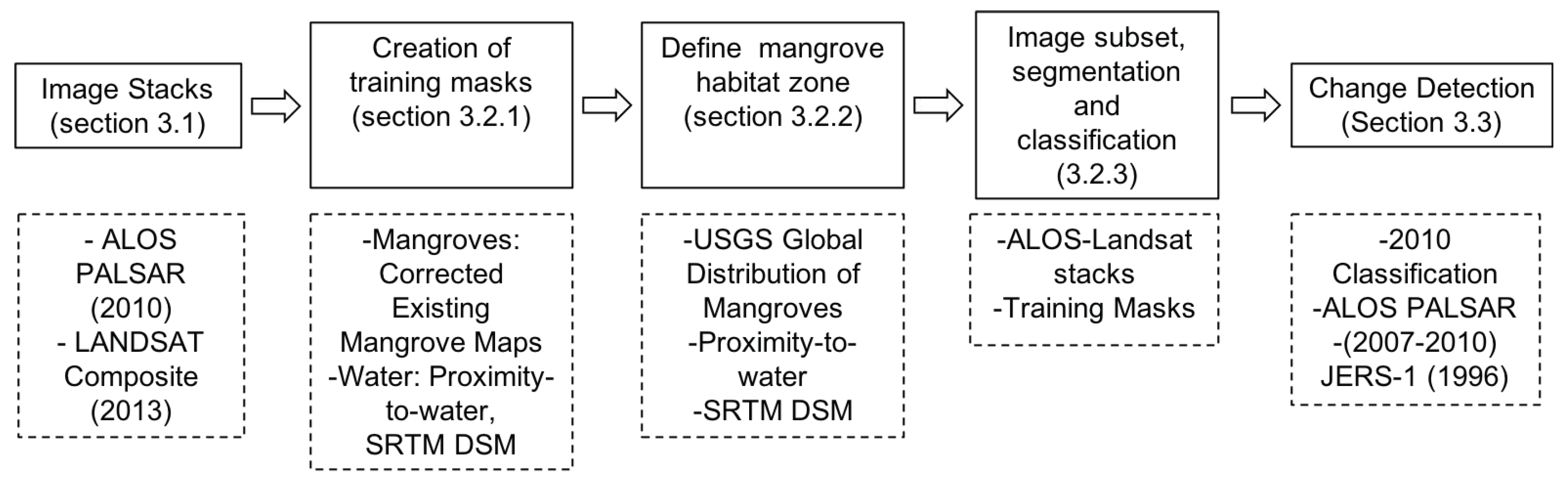
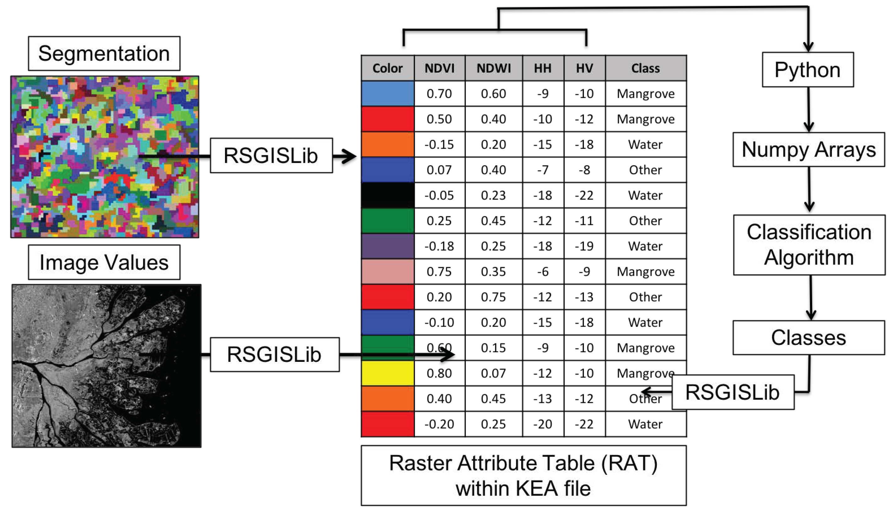
The methodology is composed of numerous interconnected steps. A high level overview of the methodology is provided in Figure 2. We used an open source Geographic Object-Oriented Image Analysis (GEOBIA) approach (Figure 3) using the Python scripting language (Python Software Foundation, https://www.python.org/). We implemented image segmentation using the Shepherd segmentation [42] and image objects were stored within a Raster Attribute Table (RAT), supported by the KEA image file format [43]. Mean statistics per object from an input image (e.g., ALOS PALSAR HV-polarization data) were populated into the image objects using commands within the Remote Sensing and GIS Library (RSGISLib) python package [44]. The statistics populated into the RAT were accessed and manipulated as a numpy array. An overview of the method is provided in Figure 2.

2.2.1. Training Data Mask

Existing maps of mangrove extent (e.g., Giri et al. [1]) were used as masks to collect training data for a new mangrove baseline. However, some of these datasets are in excess of a decade old and losses and gains in mangrove extent were removed and added to the training mask, respectively. The Giri et al. [1] (2011), WCMC updated map of mangroves (2011) [1] and World Atlas of Mangroves [34] (2010) datasets, were combined and edited at each location to form a comprehensive training library for mangroves representing all species and types. The world atlas of mangroves [33] was not incorporated due to the inaccuracy of the mangrove extent at the study site locations.

A water training mask was generated using the Geospatial Data Abstraction Library (GDAL) and RSGISLib. At each study site a threshold was set on the ALOS PALSAR HH backscatter images (<−15 dB) and on a corresponding SRTM DSM (<5 m) to identify the open water extent. A HH backscatter value greater than −15 dB erroneously included vegetation in the watermask whilst a lower value than this excluded rough water surfaces due to ocean waves. An elevation threshold of 5 m allowed inland rivers connected to the ocean to be included in the watermask. These thresholds resulted in a binary image of sea extent that also included some low lying inland water bodies (i.e., aquaculture) and flat bare regions inland, that had a low backscatter. Inland water bodies and bare ground were separated from the ocean by aggregating adjacent pixels into individual objects (clumps). The intersection of the objects with an existing lower resolution sea extent mask separated the ocean from inland water bodies and bare ground.

2.2.2. Local Mangrove Habitat Regions

Mangroves have a defined geo-spatial habitat within the intertidal zone, which, by definition is close to water and low in elevation. Here we defined the regions capable of supporting mangrove forests at each study site using elevation and proximity-to-water values derived from the SRTM DEM and a GDAL distance-to-water raster. Using Giri et al. [1], we extracted elevation and distance-to-water values specific to mangroves. To define the maximum distance-to-water value, we chose the 90th percentile of the distribution and doubled the value to generate a distance buffer that would account for the presence of mangroves outside of the known extent. All land cover from the coast (0 m inland) to this maximum value would be included in the habitat region. We defined the maximum elevation using the 99th percentile of the elevation distribution, capped at 50 m, based on previous use of the SRTM to map mangrove forests by [45]. Site specific values for maximum elevation and distance to water are available in

Table 2. The thresholds used to define the mangrove habitats for each site.

Number	Study Site	Dist to Water (m)	Max Elevation (m)
1.	Gulf of Fonesca, Honduras	10,468	50
2.	Bragança (Pará), Brazil	4928	29
3.	Sáo Luis (marahháo), Brazil	6252	35
4.	Amapá State, Brazil	42,388	30
5.	Todos os Santos, Brazil	5100	25
6.	Guayaquil, Ecuador	4996	50
7.	French Guiana	16,160	39
8.	Gulf of Paria Venezuela/Trinidad and Tobago	8918	50
9.	Guinea Bissau	9670	19
10.	Zambezia, Mozambique	31,260	18
11.	Niger delta, Nigeria	9736	23
12.	Riau, Indonesia	4702	19
13.	East Kalimantan, Indonesia	3752	17
14.	Balikpapan, Indonesia	3752	17
15.	Perak, Malaysia	4334	23
16.	Kakadu NP (NT), Australia	13,874	15

.

2.2.3. Random Forests Classifier

At each study site the Landsat-ALOS stack was subset using the local region of interest and the ALSO PALSAR HH and HV bands were segmented using the segmentation algorithm within RSGISLib [42]. A Lee filter [46] with a 3 × 3 window was used to filter the ALOS PALSAR bands prior to segmentation but non-filtered ALOS PALSAR bands were populated into the RAT to avoid over-smoothing the data. Image objects were populated with the mean value of the pixels contained within each object, for each of the four bands (HH, HV, NDVI, NDWI). These were used as input variables in a random forests classifier. The mangrove training mask and watermask were populated into the RAT to define training objects for these classes, whilst all other classes were defined as the ’other’ class. Although the imagery was subset to eliminate large numbers of objects, the quantity of training data, especially for the ‘other’ non-mangrove class, was large. We used a histogram sampling method to sub-sample the training data. All objects within the mangrove habitat region of interest were classified. We used 1000 estimators selected via sensitivity analysis, demonstrating a high out-of-bag score with little loss in processing time. A measure of variable importance within the Random Forest classifier revealed all bands to be approximately equally important across the study areas.

2.3. Change Detection

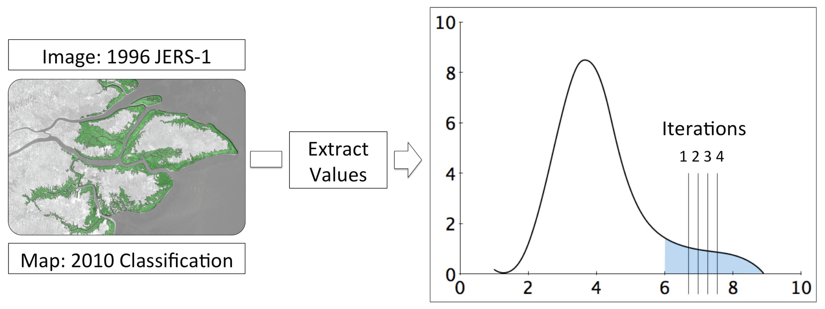
Existing approaches to change detection have used map-to-map [47] or image-to-image techniques [48,49]. Map-to-map approaches rely on the acquisition of independent classifications and therefore suffer from error propagation, whilst image-to-image approaches do not identify class level change and can be affected by differences in image calibration between scenes. To overcome these limitations, we propose a new map-to-image method of change detection whereby a map derived from one dataset is used to detect changes in a second independent image. This map-to-image approach relies upon locating anomalies in the distribution of pixel/object values within the spatial extent of a given class. The distribution of values extracted for a land cover class is assumed to be normal with deviations away from this identified as change features. The class distribution and change features are therefore separable and not both contained within one normal distribution. The majority of values that represent the class are subsequently close to the median of the dataset and the values that represent the change features are far from the median, within the tail of the distribution. Consequently, the change features compose a proportionately smaller quantity of the class than the unchanged features and separation of the tail from the distribution will identify the change features.

In this method, the selection of a threshold to locate the change features within the class distribution is critical and will vary by scene, dataset and class. As the class is normally distributed, with change features located in a tail away from the class median, the removal of the tail will normalize the class distribution. Iteratively removing the tail of a distribution in increments from the tail-end towards the median until the distribution is normal, will separate the change from the non-change objects. The normality of the distribution is calculated based upon measures of skewness and kurtosis. The tail of the distribution is iteratively removed over a user defined range using a user defined increment. The combined lowest skewness and kurtosis values identify the iteration at which the distribution is most normal and is selected as the threshold. This process is shown in Figure 4.

Annual and Decadal Changes

To detect changes between two images the values of both were populated into common image objects. For this, a segmentation that represented both images was achieved by intersecting two independent segmentations. The segments were populated with the 2010 baseline mangrove extent and water class using the mode value for each object, alongside the mean pixel value of the change-year image. ALOS PALSAR (2007–2009) and JERS-1 mosaic data (1996) were used as change-year images.

The automated detection of changes from the 2010 baseline to the JERS-1 (1996–2010) and 2010 baseline to earliest ALOS PALSAR (2007–2010) imagery was achieved, but the detection of changes between annual ALOS PALSAR imagery (2007–2008, 2008–2009, 2009–2010) was initially unsuccessful. This was due to the narrow class distribution derived from the ALOS PALSAR imagery exacerbated by the change objects typically composing <1% of the objects between consecutive ALOS years. To enhance the separability of the annual change features from the distribution, we normalized the object values between images by taking the ratio of the two scenes. The ratio of images divides one image by another, normalizing the imagery and providing a wider distribution over which to detect anomalies. This combined an image-to-image technique within a map-to-image approach. The ratio threshold was subsequently selected automatically by iteratively removing the tail of the distribution and testing its normality, but due to the consistency of the annual ALOS data [50] a value of 2.5 was selected for each class at each study site.

This defined potential change features only and were subsequently differentiated from true class changes using a number of logical contextual rules. Initially a minimum mapping unit of 1 ha and was applied to both the JERS-1 and ALOS PALSAR change features. Additional contextual rules included thresholds excluding >−20 dB backscatter on water and <−20 dB on mangrove, respectively. A 1000 m threshold on proximity between classes, for each class was also defined. This limited the anomalous detection of changes such as mangrove gain occurring far inland.

2.4. Accuracy Assessment

2.4.1. Baseline Accuracy Assessment

The baseline accuracy assessment was two-fold, composed of a combination of stratified random sampling and transects across class boundaries. A two-fold approach such as this provided a means of assessing not only the accuracy of the proportion of the image correctly classified but also provided a method of assessing the accuracy of the class boundaries. Within each of the 3 classification classes (i.e., mangrove, non-mangrove and water), a minimum of 200 points per class (600 per study site) was chosen for a total of 10,500 points. The across class tangents were manually drawn and converted to points at a 100 m interval. The number of points along a tangent varied at each site but ranged from 152 in Perak, Malaysia, to 607 in Guinea Bissau. The number of points varied by the mangrove area and complexity of the mangroves, where borders between adjacent classes were more frequent. The total number of tangent points was 5027, providing a total of 15,527 points when combined with the stratified randomly sampled points. Each of the points was buffered by 50 m to account for the difference in the classification resolution and high resolution Google Earth reference data. The accuracy of the classification is provided in

Table 3. Classification results and accuracy of classified mangrove at 16 locations across the tropics using the Random Forests algorithm.

Study Site	Area (ha)	Giri Area (ha)	Giri Difference (%)	Stratified Random Accuracy (%)	Border Accuracy (%)	Overall Accuracy (%)	Kappa	Wilson Range (%)	p-Value
Amapá state	130,870	92,900	29.0	94.3	97.4	95.5		0.90	93.9–97.0	0.019
Bragança	251,420	234,730	6.6	92.1	95.4	93.2	0.86	91.3–95.2	0.048
Sáo Luis	172,820	169,670	1.8	93.5	90.5	90.1	0.79	87.5–92.6	0.099
Biai de Todos os Santos	55,270	35,920	35.0	89.8	71.8	86.5	0.71	83.6–89.5	0.147
Guayaquil	134,130	152,100	11.3	98.0	99.6	98.5	0.97	97.4–99.6	<0.001
French Guiana	142,100	150,000	5.3	90.7	89.9	90.4	0.79	88.0–92.7	0.100
Guinea Bissau	592,990	740,430	19.9	93.9	93.3	93.7	0.86	92.1–95.2	0.046
Honduras	104,030	89,360	14.1	94.2	90.0	92.7	0.84	90.5–94.9	0.062
Mozambique	24,230	41,710	41.7	89.7	76.0	85.4	0.68	82.3–88.5	0.169
Riau	150,570	111,590	25.9	91.8	87.7	90.5	0.79	87.9–93.0	0.095
Mahakam Delta	69,980	76,980	9.1	93.7	98.1	94.6	0.88	92.5–96.7	0.032
Balikpapan	58,770	51,250	12.8	91.3	89.3	90.6	0.79	88.2–93.1	0.013
Perak	44,050	43,930	0.3	95.5	98.0	96.0	0.92	94.2–97.9	0.012
Niger delta	372,440	317,670	14.7	95.7	96.2	95.8	0.92	94.1–97.6	0.093
Kakadu	9800	21,350	54.1	97.3	95.8	97.0	0.93	95.4–98.6	0.006
Gulf of Paria	216,290	288,260	25.0	94.0	91.5	93.4	0.85	91.6–95.3	0.055
Combined	2,529,760	2,517,850	0.5	93.5	91.2	92.8	0.84	92.2–93.3	0.059

.

2.4.2. Change Detection Accuracy Assessment

The accuracy of the change detection was determined twice using two different assessments. The assessments were determined independently and the results of each are presented separately.

• The first approach assessed the accuracy of the output maps, determining their reliability for use within mangrove monitoring and determined whether a detected change was a real-world change in mangrove extent. This is referred to as the “map” accuracy assessment.
• The second approach assessed the performance of the change detection method and its ability to detect differences in time-series imagery, irrespective of the cause of the change between the two images. This is referred to as the “algorithm” accuracy assessment. This differs from the “map” accuracy assessment by not punishing the method for detecting a difference between images, even if it was not a change in mangrove extent.

The accuracy assessments were carried out by manually validating every change feature detected over the annual periods of the ALOS PALSAR imagery. Both mangrove loss and mangrove gain were assessed for the periods 2007–2010, 2007–2008, 2008–2009 and 2009–2010. In order to capture potential change features that were not detected by the method, a series of ‘no-change’ points were also validated. These no-change points were selected at random within a buffer surrounding the location where change was most likely to occur. This was within the mangrove class, in the water class within 1000 m of land, in the other class within 1000 m of the mangrove class and in the other class within 1000 m of water. This created a coastal buffer zone that included the mangrove and extended into the water and other class. Each of the validation points was buffed by 50 m to account for the difference in resolution between the ALOS PALSAR and high resolution validation imagery. This process was repeated for the JERS-1 change features but due to the larger quantity of features detected, a sample size of 300 was randomly chosen at each study site. A total of 4800 features were validated for the period 1996–2010.

3. Results

3.1. 2010 Baseline Classification

The mangrove baseline was classified at each of the 16 study sites, updating the existing extent at these locations by a decade. A total of 2,529,760 ha of mangrove forest was classified across 16 study sites, ranging from 24,230 ha in Mozambique to 592,990 ha in Guinea Bissau (Table 3). The accuracies for the individual baseline classifications were between 85.1% (Mozambique) and 98.5% (Guayaquil, Ecuador). The overall accuracy was 92.8%, with a 99% likelihood of a confidence interval between 6.7% and 7.8% using the Wilson score interval [51]. The overall accuracy was therefore in the range 92.2–93.3 with high kappa value of 0.84 and z-score p-value significant at p < 0.1. The p-value for the classification at each study site was p < 0.1 for all sites except Baia de Todos os Santos (Brazil), French Guiana and Zambezia (Mozambique).

The difference between the total area of mangrove mapped in this study and that of Giri et al. [1] was 0.5%, although there were some large discrepancies in the mangrove area at individual study sites. The difference was <10% at the Bragança coastline and Sáo Luis (Brazil), French Guiana, Guinea Bissau, the Mahakam delta (East Kalimantan, Indonesia) and Perak (Malaysia), despite a difference of at least a decade between the imagery used. Despite small differences in the mangrove forest area classified in both studies this did not mean that the extent had not changed. The difference between the mangrove areas at French Guiana was 5%, yet large areas of gain and loss in extent were mapped. Conversely, there was a large difference in the mangrove area at Amapá State (Brazil, 29%), Baia de Todos os Santos (Brazil, 39%), Mozambique (41.9%), Kakadu National Park (Australia, 54.1%) and Gulf of Paria, Venezuela (25%). Given the high accuracy of the classification, these large differences provide an accurate updated baseline at these locations, whether due to the use of an improved method or the mapping of changes in extent that had since occurred.

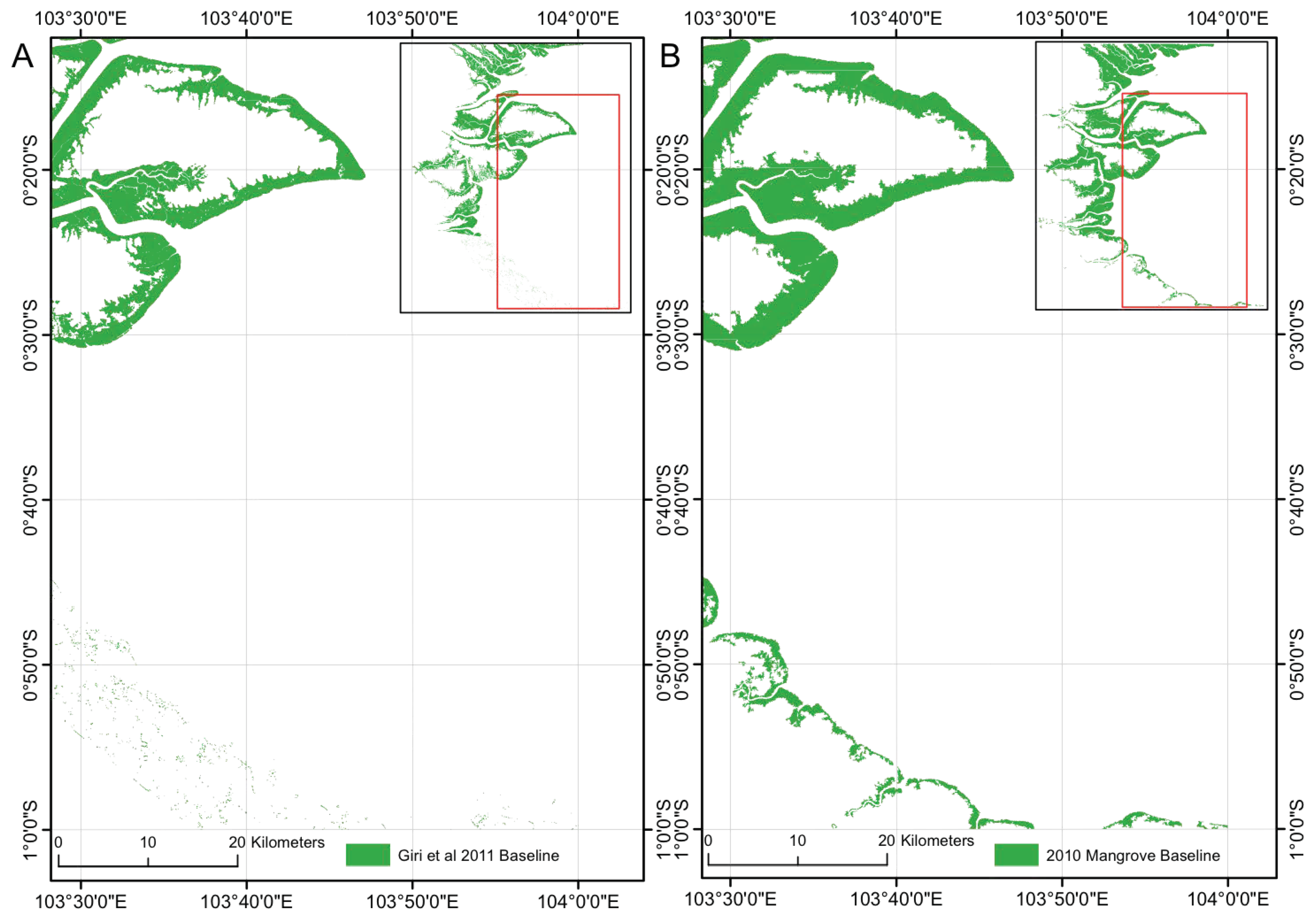
The classified extent successfully identified areas of mangrove that were omitted in the map of Giri et al. [1]. For example, at Riau, Indonesia (Figure 5) a number of false negative errors were present along the coastline accompanied by a series of false positives inland, likely to be due to cloud cover in the Landsat imagery. Despite the lack of training data for the southern portion of this region provided by the existing mask, we successfully classified all mangroves, including mangrove fringes along the coast and inland along the banks of rivers. The total mangrove area mapped for the Riau region was 25.9% larger than that classified in Giri et al. [1], with our study classifying a greater quantity of mangrove on the landward margin of the mangrove. The larger area of mangrove classified is also attributed to mangrove gain at the study site between 2000 and 2010.

3.2. Change detection

3.2.1. ALOS PALSAR 2007–2010

Over the period 2007–2010 mangrove forests at the 16 study sites experienced a combined net loss (

Table 4. Changes detected in mangrove forest extent over the period 1996–2010, 2007–2010, 2007–2008 2008–2009 and 2009–2010.

Study Site	1996–2010	1996–2010	2007–2010	2007–2010	2007–2008	2007–2008	2008–2009	2008–2009	2009–2010	2009–2010
	Gain (ha)	Loss (ha)	Gain (ha)	Loss (ha)	Gain (ha)	Loss (ha)	Gain (ha)	Loss (ha)	Gain (ha)	Loss (ha)
Amapá State	4360	7560	180	1300	10	0	30	1	1	0
Bragança	5370	3920	330	5	1	0	5	0	5	0
Sáo Luis	3260	5770	160	1280	3	4	2	0	8	2
Baia de Todos os Santos	4580	3340	3	2	2	0	1	0	4	0
Guayaquil	10,170	5280	600	870	1	0	4	0	7	0
French Guiana	15,570	8570	3250	3120	8	0	70	0	60	20
Guinea Bissau	47,930	28,420	2090	1510	9	20	50	2	120	0
Honduras	8560	2620	540	490	10	20	10	4	20	0
Mozambique	740	820	20	240	0	0	1	0	7	0
Riau	5060	950	390	240	0	0	30	0	20	1
Mahakam delta	1490	23,003	990	920	2	0	70	0	4	0
Balikpapan	2820	3950	5	320	3	0	6	0	7	0
Perak	1050	240	50	70	0	0	3	0	2	0
Niger delta	9660	1170	980	70	3	0	2	0	10	0
Kakadu	2210	570	30	40	1	0	10	0	7	0
Gulf of Paria	5160	3360	580	620	0	0	7	0	7	0
Total	127,990	76,860	10,198	11,097	53	44	301	7	289	41

), in keeping with observed trends in mangrove extent [27]. The gains and losses in extent were small in comparison to the total mangrove area (2,529,760 ha) mapped, but accounted for a substantially large proportion of mangrove area in some regions (i.e., the Mahakam delta, East Kalimantan, Indonesia). The largest change observed was in French Guiana where 3250 ha of mangrove gain occurred between 2007 and 2010. The largest loss of mangrove counterbalanced this at French Guiana where 3120 ha of mangrove was lost over the same period. The smallest changes were observed at Baia de Todos os Santos, Brazil, where 3 ha of mangrove gain and 2 ha of mangrove loss were observed between 2007 and 2010. The “map” accuracy (

Table 5. “Map” accuracy of changes detected in mangrove forest extent over the period 1996–2010, 2007–2010, 2007–2008 2008–2009 and 2009–2010.

Study Site	1996–2010	1996–2010	2007–2010	2007–2010	2007–2008	2007–2008	2008–2009	2008–2009	2009–2010	2009–2010
	Gain (%)	Loss (%)	Gain (%)	Loss (%)	Gain (%)	Loss (%)	Gain (%)	Loss (%)	Gain (%)	Loss (%)
Amapá State	78.0	71.8	88.5	73.8	100	96.8	98.9	96.8	100	96.8
Bragança	66.4	70.2	79.6	74.3	100	98.0	100	98.0	99.6	98.0
Sáo Luis	61.0	69.6	96.8	68.2	100	96.0	98.8	96.8	99.2	96.5
Baia de Todos os Santos	64.0	47.4	93.8	91.8	100	92.4	99.6	92.4	99.6	92.4
Guayaquil	61.9	84.0	69.1	76.4	99.7	96.8	98.1	96.8	99.0	96.8
French Guiana	69.6	79.2	85.4	96.2	100	100	99.3	100	98.5	98.8
Guinea Bissau	67.8	50.0	84.5	74.5	99.3	91.8	98.3	93.6	95.8	93.6
Honduras	66.5	93.2	70.5	88.0	100	96.1	100	96.8	97.8	96.8
Mozambique	58.9	58.3	95.6	89.7	100	94.4	100	94.4	98.4	94.4
Riau	57.6	52.0	84.5	69.6	100	95.2	98.5	95.2	99.6	94.8
Mahakam delta	68.0	83.2	94.2	88.2	100	98.4	94.4	98.4	99.7	98.4
Balikpapan	57.4	85.8	80.1	93.9	100	98.4	99.6	98.4	100	98.4
Perak	52.8	79.1	97.7	88.2	100	94.0	100	94.0	100	94.0
Niger delta	50.4	54.3	55.8	52.9	99.2	99.7	100	99.7	100	99.7
Kakadu	59.6	66.9	87.5	94.7	99.6	96.0	100	96.0	99.2	96.0
Gulf of Paria	62.0	53.0	67.4	67.2	100	98.8	100	98.8	100	98.8
Total	62.7	68.3	81.5	78.3	99.9	96.5	99	96.7	99.1	96.5
Kappa	0.24	0.35	0.53	0.45	0.89	NA	0.86	NA	0.84	NA
Wilson Range (%)	61.3–64.0	66.9–69.7	80.2–82.7	77.0–79.7	99.7–100	96.7–97.2	98.6–99.4	95.9–97.4	98.8–99.5	95.8–97.3

) of the detected changes varied from 50% (Guinea Bissau) to 100% (Balikpapan, Perak) although the “algorithm” accuracies (

Table 6. “Algorithm” accuracy of changes detected in mangrove forest extent over the period 1996–2010, 2007–2010, 2007–2008 2008–2009 and 2009–2010.

Study Site	1996–2010	1996–2010	2007–2010	2007–2010	2007–2008	2007–2008	2008–2009	2008–2009	2009–2010	2009–2010
	Gain (%)	Loss (%)	Gain (%)	Loss (%)	Gain (%)	Loss (%)	Gain (%)	Loss (%)	Gain (%)	Loss (%)
Amapá State	94.6	93.0	93.9	96.3	100	96.8	97.4	96.8	100	96.8
Bragança	95.4	72.8	91.0	96.6	100	98.0	100	98.0	100	98.0
Sáo Luis	95.0	96.0	99.6	96.3	100	96.8	98.1	96.8	99.2	96.5
Baia de Todos os Santos	90.0	94.4	96.7	92.6	100	92.4	100	92.4	99.6	92.4
Guayaquil	95.0	85.2	95.5	96.6	100	96.8	99.7	96.8	99.3	96.8
French Guiana	88.8	96.6	97.9	99.5	100	100	99.3	100	98.2	98.2
Guinea Bissau	97.5	95.4	91.5	93.4	99.3	92.2	97.7	93.6	95.2	93.6
Honduras	95.5	94.4	92.9	97.6	100	96.1	100	96.8	97.8	96.8
Mozambique	93.9	95.3	98.6	93.8	100	94.4	100	94.4	98.8	94.4
Riau	91.4	95.6	92.0	95.1	100	95.2	98.5	95.2	99.6	95.2
Mahakam delta	98.3	97.2	95.9	97.8	100	98.4	94.5	98.4	99.7	98.4
Balikpapan	95.4	95.7	94.4	98.2	100	98.4	99.2	98.4	100	98.4
Perak	81.6	94.7	100	92.9	100	94.0	99.6	94.0	100	94.0
Niger delta	99.8	99.8	90.0	98.8	100	99.7	100	99.7	98.1	99.7
Kakadu	97.6	96.0	97.4	96.2	99.6	96.0	100	96.0	100	96.0
Gulf of Paria	93.8	97.0	96.5	98.3	100	98.8	99.6	98.8	99.6	98.8
Total	94.0	93.7	94.9	96.5	99.9	96.5	98.9	96.7	99	96.6
Kappa	0.88	0.87	0.88	0.92	0.95	NA	0.84	NA	0.81	NA
Wilson Range (%)	93.3–94.7	92.9–94.4	94.2–95.6	95.9–97.1	99.8–100	95.8–97.3	98.5–99.3	95.9–97.4	98.6–99.4	95.8–97.3

) were all in excess of 80%, with confidence intervals at 99% likelihood. This demonstrated that the method was successfully able to detect differences in image objects over a given period but that the change detected was not always due to a change in mangrove extent. Image misresgistration or rough water surfaces caused by waves could be the cause of the lower ‘map’ accuracies observed. This was exacerbated when these false positives made up a significant proportion of the total change features. The combined accuracy of the detected changes was evaluated per year, where changes in excess of a minimum threshold of 50 ha occurred. Change areas below this were not able to provide a representative quantity sufficient to derive a robust statistics. This highlighted an inadequacy of the system to monitor change over a very short period, with 0 ha of change regularly detected over an annual period. Over an annual period, the sum of the changes between 2007–2008, 2008–2009 and 2009–2010 did not match the total gain and loss observed between 2007–2010.

3.2.2. JERS-1 SAR/ALOS PALSAR 1996–2010

Mangrove forests over the period 1996–2010 experienced a net gain in extent at the study sites (Table 4). The total mangrove gain detected over the period was 127,990 ha with the greatest gain occurring at French Guiana whereby 15,570 ha of mangrove was gained and was offset by 8570 ha of loss, caused by natural changes in extent along the coastline. Larger changes in extent were observed at Guinea Bissau but misregistration caused ’map’ errors to be as large as 50%. The greatest loss in extent measured over the period was at the Mahakam delta, East Kalimantan, where 32,003 ha of loss was mapped. The success of the method enabled change detection to be carried out over a large temporal range at high spatial resolution with a difference between the JERS-1 imagery and the mangrove baseline classification of 14 years.

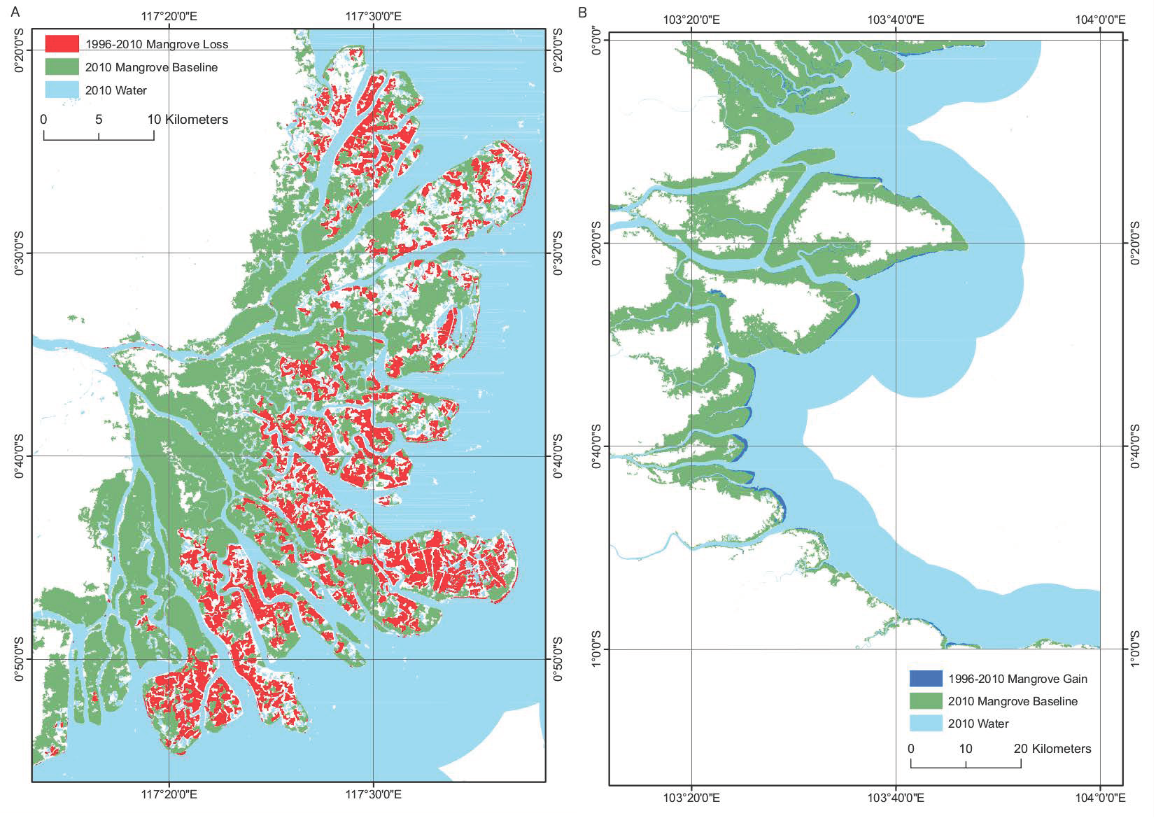
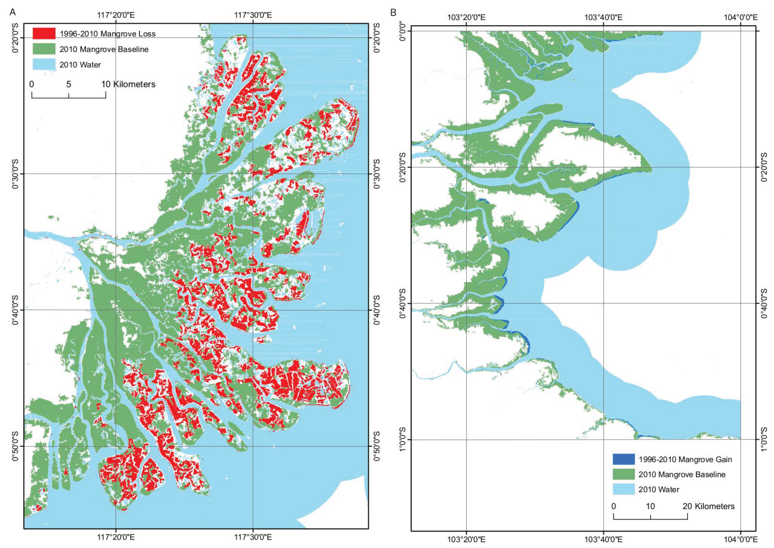
The mangroves of the Mahakam delta, East Kalimantan, have been historically heavily disturbed due to the installation of aquaculture, causing the removal of large areas of mangrove [29,52]. The proposed method was able to successfully detect this loss of mangrove due to the contrast in backscatter between the mangrove forest and the surface of the aquaculture pond. This is because the water surface of an aquaculture pond promotes specular backscatter whilst a mangrove forest promotes diffuse backscatter, causing large differences in the backscatter of the two land cover types in radar imagery. This demonstrates the ability of the method to highlight changes in mangrove extent as a direct consequence of anthropogenic activity and the ability of the method to provide users with knowledge on human induced forest loss. The mangrove loss at the Kalimantan delta over the period 1996–2010 was 23,003 ha with a small quantity of gain of 1490 ha (Figure 6). Conversely, the method was also able to successfully detect increases in the mangrove forest extent. Advances in mangrove forest extent were previously detected at Riau, Indonesia [53] and were successfully detected in this study (Figure 6). The method was capable of achieving results with overall “map” accuracies (Table 5) for the mangrove gain of 62.7% and mangrove loss of 68.3% and high “algorithm” accuracies (Table 6) for mangrove gain and loss of 94.0% and 93.7%, respectively. As with the ALOS PALSAR change detection the low ’map’ accuracies were caused by image registration error and anomalous changes in object values (e.g., rough water).

4. Discussion

This paper demonstrates a method for updating mangrove baseline extents across the tropics. An object-oriented machine learning approach was able to successfully classify mangrove forest extent across a variety of mangrove environments, ranging from large continuous forests (Riau) to small extents (Baia de Todos os Santos) and fragmented stands (Mahakam delta). A novel map-to-image change detection approach was demonstrated to be capable of updating these baselines over multi-year (2007–2010) to decadal (1996–2010) periods, by successfully detecting both large and small changes in extent whilst being robust against false positives. This combined system provides a means of implementing a mangrove monitoring system, applicable at the global scale.

4.1. Baseline Classification

Mangrove baselines were updated from the existing global extent by over a decade using a globally applicable approach. The method successfully mapped mangrove extent without the requirement for modification at each study site, representing a single holistic and globally applicable approach to mangrove mapping. This method was able to achieve accuracies in excess of 90% and was able to improve upon the existing mangrove dataset [1], by successfully mapping previously omitted portions of extent (Figure 5). The method was not limited to the extent of existing datasets and was able to demonstrate this by classifying mangrove extent outside of currently mapped baselines. This offers an advantage over existing monitoring systems [25] whist simultaneously improving the mangrove baseline at those discrete locations, at a comparable resolution to existing maps [1]. The accuracy of the mangrove baseline at Baia de Todos os Santos, French Guiana and Mozambique were not significant due to the lower accuracies of the baselines. These baselines are not as reliable as those significant at p < 0.1, but with accuracies all in excess of 80% represent maps of sufficient quality for use within the research community and policy making. The cause of this lower accuracy was a similarity in backscatter and reflectance between mangrove and non-mangrove land cover types, resulting in either an over- or underestimation of the mangrove baseline. Despite this, the classification accuracy at each study site was high (>80%) and the overall classification accuracy of 92.8% maintains that the method was robust for mapping mangrove extent at the global scale. The accuracy and scale (1 ha) of the generated maps ensure that they are suitable for informing both local and regional management strategies, whilst satisfying the requirements for global initiatives, including Payment for Ecosystem Services (PES) schemes [6]. The baseline year (2010) was chosen as to coincide with the best available data, subsequently yielding an updated but not up-to-date baseline. The baseline should therefore be considered as the initial stage (t0) of a monitoring system and as the most recent but not final product. The development of an automated processing chain positions this work as the primary method for use in generating an updated global mangrove baseline map, such as within the Global Mangrove Watch project [40] required by the research community, stakeholders and local mangrove initiatives.

The high accuracies of the baselines were quantifiable despite covering very large geographical areas. Existing large scale maps [1,39] do not provide estimates of accuracy, at the local nor global scale. This was achieved at each of the study sites mapped, providing both local and global estimates of accuracy. This is an important improvement in the field of large scale extent mapping through the provision of a robust accuracy assessment which has been demonstrated across very large geographical areas and is therefore applicable for use at a global scale. The successful classification and differentiation of mangroves from other land cover classes, demonstrated that mangrove extent could be accurately classified using four image bands (two optical, two radar) and did not require the full range of multispectral optical imagery. The use of normalized indices offered an advantage of using top of atmosphere (TOA) imagery, negating the requirement for atmospheric correction. The causes of error within the baseline maps were limited. The spectral similarity of vegetation classes was a source of error, particularly where wetland forests adjoined mangroves. The similarity in spectral response and backscatter was unable to differentiate these classes. This was exacerbated in regions where the Landsat mosaic was inhibited by excessive cloud cover and a fragmented composite image was created.

The combination of optical and radar data enabled the different modalities to complement one another and provide the classifier with different information. Optical data was able to provide information on the chemical and biophysical composition of the land cover classes whilst radar data provided information on their structure. This has been been previously observed to yield an increase in accuracy in excess of 20% by using a combination of optical and radar datasets than when used independently [54,55]. Fusing data of different modalities has been demonstrated to improve accuracy [56,57,58,59], although the combination of optical and SAR has received little attention for mangrove mapping, especially at large scales. Nevertheless, this has been previously achieved over large areas with accuracies of 93.91%, and 83% reported for estimates of height, biomass and carbon [45,60]. Additional studies [61,62,63,64,65] that utilise a combination of radar data with optical data or another radar dataset do not provide quantitative assessments of accuracy. This further reflects the lack of data available in this field for conducting rigorous accuracy assessments of mangroves over large geographical areas and highlights the advance made in this work to provide this confidence in the baseline and change maps.

The Random Forests algorithm was able to adequately and accurately classify mangrove extent and differentiate it from other land cover classes at a variety of locations, with no modification of the algorithm parameters required furthering the global applicability of the method [66]. The use of the Random Forests algorithm was advantageous given that the training data was contained within a small number of classes composed of a number of sub-classes. The mangrove class contained mangrove of different growth stages and species whilst the ‘other’ class was composed of a large number of classes with a broad range of spectral and backscatter object values. This markedly improved the efficiency of the collection of training data for the classifier whilst resulting in high accuracies that have been observed for random forests and decision tree classifiers [67,68,69]. A GEOBIA framework has not been widely used for mangrove mapping [70] yet offers a variety of benefits over per-pixel classifications [71] and has been observed to achieve higher accuracies [72,73]. This was demonstrated in this work by reducing the noise associated with radar imagery due to speckle and providing the mangrove forests with context within their environment (e.g., distance to water). The segmentation was able to use the radar to form image objects that represented real world features, that had common HH and HV backscatter values. This reduced the granularity of the classification that is present in per-pixel classifications.

4.2. Change Detection

Changes in mangrove forest extent were mapped using a novel map-to-image approach that was demonstrated to be capable of mapping change features from both the same and different sensors from which the classification was derived. This offered a number of advantages over existing methods that include map-to-map and image-to-image methods [74,75]. The map-to-image change detection utilized an image-to-image technique to enhance the detection of change features between images acquired by the same sensor. This provides the method with additional flexibility and applicability and demonstrates that a range of inputs can be used for the detection of change features. As the change threshold is calculated automatically, this provides an additional advantage of the map-to-image approach over existing methods [48,49]. Furthermore, the map-to-image method is not limited to a specific land cover class and thus has a wide applicability in the field of change detection.

Inventories and extent maps are quickly outdated when driven by the loss of mangrove on the magnitude observed over the past half century [26] and require a method of being readily updated. The baseline map forms the basis of a monitoring system from which gains and losses in mangrove extent can be mapped. The map-to-image method subsequently enables baselines to be updated using available current data in an automated method applicable at the global scale. It is able to facilitate this through its ability to detect changes irrespective of the input dataset type (e.g., optical, radar, lidar), guaranteeing constantly available datasets for monitoring mangrove extents and updating mangrove baselines. This is particularly pertinent with the forthcoming radar (e.g., NISAR, ALOS4) and current and near future optical satellites (e.g., Sentinel-2, Landsat 8/9) planned by a variety of international space agencies and collaborations. An integrated change detection approach like this enabled the baseline to be derived for the period when the best data, and not most recent data, was available. This benefited this study by allowing a baseline for 2010 to be generated, from which changes could be mapped, forming a new baseline. Our study maps historical changes, but can be updated to form a baseline for any year at any scale (local, regional, global) as required. Consequently, we present a globally applicable approach to mangrove extent and change mapping suitable for use as a global monitoring system.

The mangrove forests at several of the selected study sites were shown to have an overall increase in extent over the period 1996-2010, which defies the trends observed in global mangrove forests [76]. The study sites were selected as they represented a range of static and dynamic systems with variable mangrove ecosystems, therefore providing locations in which the change detection system could be tested. As such, they represent a biased sample that do not necessarily reflect the global trends in mangrove change. The map-to-image approach was shown to adequately (>90%) detect changes in image classes, irrespective of the type of the driver or geographical setting. The detection of changes was limited to the seaward margin or where large contrasts between images were present. As such, smaller scale changes at the landward margin, such as the conversion of mangroves by terrestrial land cover types, were not detected as they did not produce a sufficient backscatter response to be detected as change from mangrove forest land cover type. The map-to-image approach could target such changes provided other modes of data (multi-, hyperspectral) that are sensitive to changes in spectral response [77] are utilized. The accuracy of the mangrove change maps (“map” accuracies) were lower than that of the “algorithm” accuracies. This was primarily a consequence of poor image registration at some locations which would need to be rectified in order to use ALOS PALSAR/JERS-1 for assessments of change in mangrove extent. Similarly, the map-to-image method was not able to generate reliable annual maps of change. Due to the minimum mapping unit (1 ha), changes occurring on this scale annually were not common and the detection of false positives were more common. To address the needs of policy, change maps covering 5-year periods could satisfy the requirements of a number of international targets and treaties. These include the Ramsar Convention, the UNFCCC, Convention of Biological Diversity (CBD) and Aichi targets 5, 7, 11, 14 and 15 [6]. Changes in extent were detected using archival radar data and can be continued with existing (i.e., ALOS-2 PALSAR-2) and forthcoming (e.g., NISAR) missions. This has an advantage over previous methods of change detection that required existing mapped products (e.g., forest change maps) were available [25]. As such, the map-to-image approach represents an important development in field of land cover change detection.

This approach has outlined the basis of the methodology used by the Global Mangrove Watch to achieve an updated global mangrove forest baseline for the year 2010 [40] available via the Global Forest Watch (https://www.globalforestwatch.org). This will deliver annual maps of mangrove forest extent and change using ALOS PALSAR and ALOS-2 PALSAR-2 data for 2018 and into the future. These products could be used in conjunction with currently available biomass data [45,78] to map and monitor the spatial distribution of biomass currently held within these ecosystems. A continued monitoring system is recommended given the importance of these ecosystems on an at least 5-year monitoring period.

5. Conclusions

This study provides the first holistic approach to large scale mangrove mapping, capable of achieving a global baseline classification and monitoring system. The existing mangrove baseline was updated at a selection of study sites, mapping 2,529,760 ha of mangrove with an accuracy >90% using a Random Forests classifier. A novel map-to-image approach was used to map decadal changes in mangrove extent at accuracies in excess of 90% using globally available radar data. The approach outlines a method that is capable of using a suite of currently available and projected spaceborne sensors, at high temporal resolution, ensuring its continued capability into the future. It is important that mangrove change products are tied closely with additional ancillary data on the provision of ecosystem services and that emphasis is placed on quantifying the important ecosystem services that mangrove forests provide in monetary terms, thereby forging an economic counterbalance to the heavy pressures from a lucrative aquaculture industry. It is recommended that a mangrove monitoring system is established with global change products made available on a 5-year basis.

References

- Giri, C.; Ochieng, E.; Tieszen, L.L.; Zhu, Z.; Singh, A.; Loveland, T.; Masek, J.; Duke, N. Status and distribution of mangrove forests of the world using earth observation satellite data. Glob. Ecol. Biogeogr. 2011, 20, 154–159. [Google Scholar] [CrossRef]
- Jennerjahn, T.C.; Ittekkot, V. Relevance of mangroves for the production and deposition of organic matter along tropical continental margins. Naturwissenschaften 2002, 89, 23–30. [Google Scholar] [CrossRef] [PubMed]
- Donato, D.C.; Kauffman, J.B.; Murdiyarso, D.; Kurnianto, S.; Stidham, M.; Kanninen, M. Mangroves among the most carbon-rich forests in the tropics. Nat. Geosci. 2011, 4, 293–297. [Google Scholar] [CrossRef]
- Murray, B.C.; Pendleton, L.; Jenkins, W.A.; Sifleet, S. Green Payments for Blue Carbon: Economic Incentives for Protecting Threatened Coastal Habitats; Nicholas Institute for Environmental Policy Solutions, Duke University: Durham, NC, USA, 2011; NI R 11-04. [Google Scholar]
- Hamilton, S.E.; Friess, D.A. Global carbon stocks and potential emissions due to mangrove deforestation from 2000 to 2012. Nat. Clim. Chang. 2018, 8, 240. [Google Scholar] [CrossRef]
- Lucas, R.; Robelo, L.; Fatoyinbo, L.; Rosenqvist, A.; Itoh, T.; Shimada, M.; Simard, M.; Souza-Filho, P.; Thomas, N.; Trettin, C.; et al. Contribution of L-band SAR to Systematic Global Mangrove Monitoring. Mar. Freshw. Res. 2014, 65, 589–603. [Google Scholar] [CrossRef]
- Blaber, S.J.M.; Milton, D.A. Species composition, community structure and zoogeography of fishes of mangrove estuaries in the Solomon Islands. Mar. Biol. 1990, 105, 259–267. [Google Scholar] [CrossRef]
- Frusher, S.D.; Giddins, R.L.; Smith, T.J. Distribution and abundance of grapsid crabs (Grapsidae) in a mangrove estuary: Effects of sediment characteristics, salinity tolerances, and osmoregulatory ability. Estuaries 1994, 17, 647–654. [Google Scholar] [CrossRef]
- Rasmussen, A.R.; Murphy, J.C.; Ompi, M.; Gibbons, J.W.; Uetz, P. Marine reptiles. PLoS ONE 2011, 6, e27373. [Google Scholar] [CrossRef] [PubMed]
- Platt, S.G.; Thorbjarnarson, J.B. Population status and conservation of Morelet’s crocodile, Crocodylus moreletii, in northern Belize. Biol. Conserv. 2000, 96, 21–29. [Google Scholar] [CrossRef]
- Angelici, F.M.; Politano, E.; Bogudue, A.J.; Luiselli, L. Distribution and habitat of otters (Aonyx capensis and Lutre maculicollis) in souuthern Nigeria. Ital. J. Zool. 2005, 72, 223–227. [Google Scholar] [CrossRef]
- Nowak, K. Frequent water drinking by zanzibar red colobus (Procolobus kirkii) in a mangrove forest refuge. Am. J. Primatol. 2008, 70, 1081–1092. [Google Scholar] [CrossRef] [PubMed]
- Dahdouh-Guebas, F.; Jayatissa, L.P.; Di Nitto, D.; Bosire, J.O.; Lo Seen, D.; Koedam, N. How effective were mangroves as a defence against the recent tsunami? Curr. Biol. 2005, 15, R443–R447. [Google Scholar] [CrossRef] [PubMed]
- Gopal, B.; Chauhan, M. Biodiversity and its conservation in the Sundarban mangrove ecosystem. Aquatic Sci. 2006, 68, 338–354. [Google Scholar] [CrossRef]
- Field, C.D. Impact of expected climate change on mangroves. Hydrobiologia 1995, 295, 75–81. [Google Scholar] [CrossRef]
- Bandaranayake, W.M. Traditional and medicinal uses of mangroves. Mangroves Salt Marshes 1998, 2, 133–148. [Google Scholar] [CrossRef]
- Nfotabong-Atheull, A.; Din, N.; Koum, L.G.E.; Satyanarayana, B.; Koedam, N.; Dahdouh-Guebas, F. Assessing forest products usage and local residents’ perception of environmental changes in peri-urban and rural mangroves of Cameroon, Central Africa. J. Ethnobiol. Ethnomed. 2011, 7, 41–53. [Google Scholar] [CrossRef] [PubMed]
- Ewel, K.C.; Twilley, R.R.; Eong, J.I.N.; Usda, O.N.G.; Service, F. Different kinds of mangrove forests provide different goods and services AMONG among mangrove forests. Glob. Ecol. Biogeogr. Lett. 1998, 7, 83–94. [Google Scholar] [CrossRef]
- Walton, M.; Samonte-Tan, G.; Primavera, J.; Edwards-Jones, G.; Le Vay, L. Are mangroves worth replanting? The direct economic benefits of a community-based reforestation project. Environ. Conserv. 2006, 33, 335–343. [Google Scholar] [CrossRef]
- Alongi, D.M. Mangrove forests: Resilience, protection from tsunamis, and responses to global climate change. Estuar. Coast. Shelf Sci. 2008, 76, 1–13. [Google Scholar] [CrossRef]
- Danielsen, F.; Sørensen, M.K.; Olwig, M.F.; Selvam, V.; Parish, F.; Burgess, N.D.; Hiraishi, T.; Karunagaran, V.M.; Rasmussen, M.S.; Hansen, L.B.; et al. The Asian tsunami: A protective role for coastal vegetation. Science 2005, 310, 643. [Google Scholar] [CrossRef] [PubMed]
- Barbier, E.B.; Hacker, S.D.; Kennedy, C.; Koch, E.W.; Stier, A.C.; Silliman, B.R. The value of estuarine and coastal ecosystem services. Ecol. Monogr. 2011, 81, 169–193. [Google Scholar] [CrossRef] [Green Version]
- Barbier, E.B. Valuing the storm protection service of estuarine and coastal ecosystems. Ecosyst. Serv. 2015, 11, 32–38. [Google Scholar] [CrossRef]
- FAO. The world’s mangroves 1980–2005; Technical Report; Food and Agriculture Organization of the United Nations: Rome, Italy, 2007. [Google Scholar]
- Hamilton, S.E.; Casey, D. Creation of a high spatio-temporal resolution global database of continuous mangrove forest cover for the 21st century (CGMFC-21). Glob. Ecol. Biogeogr. 2016, 25, 729–738. [Google Scholar] [CrossRef] [Green Version]
- Alongi, D.M. Present state and future of the world’s mangrove forests. Environ. Conserv. 2002, 29, 331–349. [Google Scholar] [CrossRef]
- Valiela, I.; Bowen, J.L.; York, J.K. Mangrove Forests: One of the World’s Threatened Major Tropical Environments. BioScience 2001, 51, 807–815. [Google Scholar] [CrossRef]
- FAO. The State of World Fisheries and Aquaculture 2016. Contributing to Food Security and Nutrition for All; FAO: Rome, Italy, 2016; 200p. [Google Scholar]
- Thomas, N.; Lucas, R.; Bunting, P.; Hardy, A.; Rosenqvist, A.; Simard, M. Distribution and drivers of global mangrove forest change, 1996–2010. PLoS ONE 2017, 12, e0179302. [Google Scholar] [CrossRef] [PubMed]
- Richards, D.R.; Friess, D.A. Rates and drivers of mangrove deforestation in Southeast Asia, 2000–2012. Proc. Natl. Acad. Sci. USA 2016, 113, 344–349. [Google Scholar] [CrossRef] [PubMed]
- Souza Filho, P.W.M.; Farias Martins, E.D.S.; da Costa, F.R. Using mangroves as a geological indicator of coastal changes in the Bragança macrotidal flat, Brazilian Amazon: A remote sensing data approach. Ocean Coast. Manag. 2006, 49, 462–475. [Google Scholar] [CrossRef]
- Mitchell, A.L.; Lucas, R.M.; Donnelly, B.E.; Pfitzner, K.; Milne, A.K.; Finlayson, M. A new map of mangroves for Kakadu National Park, Northern Australia, based on stereo aerial photography. Aquatic Conserv. Mar. Freshw. Ecosyst. 2007, 17, 446–467. [Google Scholar] [CrossRef]
- Spalding, M.; Blasco, F.; Field, C. World Mangrove Atlas; International Society for Mangrove Ecosystems: Okinawa, Japan, 1997. [Google Scholar]
- Spalding, M. World Atlas of Mangroves; Routledge: Abingdon, Oxon, UK, 2010. [Google Scholar]
- Friess, D.A.; Webb, E.L. Variability in mangrove change estimates and implications for the assessment of ecosystem service provision. Glob. Ecol. Biogeogr. 2014, 23, 715–725. [Google Scholar] [CrossRef]
- Ruiz-Luna, A.; Acosta-Velázquez, J.; Berlanga-Robles, C.A. On the reliability of the data of the extent of mangroves: A case study in Mexico. Ocean Coast. Manag. 2008, 51, 342–351. [Google Scholar] [CrossRef]
- Mejía-Rentería, J.C.; Castellanos-Galindo, G.A.; Cantera-Kintz, J.R.; Hamilton, S.E. A comparison of Colombian Pacific mangrove extent estimations: Implications for the conservation of a unique Neotropical tidal forest. Estuar. Coast. Shelf Sci. 2018, 212, 233–240. [Google Scholar] [CrossRef]
- Olson, D.M.; Dinerstein, E.; Wikramanayake, E.D.; Burgess, N.D.; Powell, G.V.N.; Underwood, E.C.; D’amico, J.A.; Itoua, I.; Strand, H.E.; Morrison, J.C. Terrestrial Ecoregions of the World: A New Map of Life on Earth A new global map of terrestrial ecoregions provides an innovative tool for conserving biodiversity. BioScience 2001, 51, 933–938. [Google Scholar] [CrossRef]
- Hansen, M.C.; Potapov, P.V.; Moore, R.; Hancher, M.; Turubanova, S.A.; Tyukavina, A.; Thau, D.; Stehman, S.V.; Goetz, S.J.; Loveland, T.R. High-resolution global maps of 21st-century forest cover change. Science 2013, 342, 850–853. [Google Scholar] [CrossRef] [PubMed]
- Bunting, P.; Rosenqvist, A.; Lucas, R.; Rebelo, L.; Hilarides, L.; Thomas, N.; Hardy, A.; Itoh, T.; Shimada, M.; Finlayson, M. The Global Mangrove Watch—A New 2010 Global Baseline of Mangrove Extent. Remote Sens. 2018. In submission. [Google Scholar]
- Pre-Processing of Landsat and RapidEye Data. Available online: https://arcsi.remotesensing.info (accessed on 13 September 2018).
- Clewley, D.; Bunting, P.; Shepherd, J.; Gillingham, S.; Flood, N.; Dymond, J.; Lucas, R.; Armston, J.; Moghaddam, M. A python-based open source system for geographic object-based image analysis (GEOBIA) utilizing raster attribute tables. Remote Sens. 2014, 6, 6111–6135. [Google Scholar] [CrossRef]
- Bunting, P.; Gillingham, S. The KEA image file format. Comput. Geosci. 2013, 57, 54–58. [Google Scholar] [CrossRef]
- Bunting, P.; Clewley, D.; Lucas, R.M.; Gillingham, S. The Remote Sensing and GIS Software Library (RSGISLib). Comput. Geosci. 2014, 62, 216–226. [Google Scholar] [CrossRef]
- Fatoyinbo, T.E.; Simard, M. Height and biomass of mangroves in Africa from ICESat/GLAS and SRTM. Int. J. Remote Sens. 2013, 34, 668–681. [Google Scholar] [CrossRef]
- Lee, J.S. Digital image enhancement and noise filtering by use of local statistics. Pattern Anal. Mach. Intell. IEEE Trans. 1980, PAMI-2, 165–168. [Google Scholar] [CrossRef]
- Dingle Robertson, L.; King, D.J. Comparison of pixel- and object-based classification in land cover change mapping. Int. J. Remote Sens. 2011, 32, 1505–1529. [Google Scholar] [CrossRef]
- Bruzzone, L.; Prieto, D.F. Automatic analysis of the difference image for unsupervised change detection. Geosci. Remote Sens. IEEE Trans. 2000, 38, 1171–1182. [Google Scholar] [CrossRef]
- Bruzzone, L.; Prieto, D.F. An adaptive semiparametric and context-based approach to unsupervised change detection in multitemporal remote-sensing images. Image Proc. IEEE Trans. 2002, 11, 452–466. [Google Scholar] [CrossRef] [PubMed] [Green Version]
- Shimada, M.; Itoh, T.; Motooka, T.; Watanabe, M.; Shiraishi, T.; Thapa, R.; Lucas, R. New global forest/non-forest maps from ALOS PALSAR data (2007–2010). Remote Sens. Environ. 2014, 155, 13–31. [Google Scholar] [CrossRef]
- Wilson, E.B. Probable Inference, the Law of Succession, and Statistical Inference. J. Am. Stat. Assoc. 1927, 22, 209–212. [Google Scholar] [CrossRef]
- Rahman, A.F.; Dragoni, D.; Didan, K.; Barreto-Munoz, A.; Hutabarat, J.A. Detecting large scale conversion of mangroves to aquaculture with change point and mixed-pixel analyses of high-fidelity MODIS data. Remote Sens. Environ. 2013, 130, 96–107. [Google Scholar] [CrossRef]
- Thomas, N.; Lucas, R.; Itoh, T.; Simard, M.; Fatoyinbo, L.; Bunting, P.; Rosenqvist, A. An approach to monitoring mangrove extents through time-series comparison of JERS-1 SAR and ALOS PALSAR data. Wetl. Ecol. Manag. 2015, 23, 3–17. [Google Scholar] [CrossRef]
- Held, A.; Ticehurst, C.; Lymburner, L.; Williams, N. High resolution mapping of tropical mangrove ecosystems using hyperspectral and radar remote sensing. Int. J. Remote Sens. 2003, 24, 2739–2759. [Google Scholar] [CrossRef]
- Ramsey, E.W., III; Nelson, G.A.; Sapkota, S.K. Classifying coastal resources by integrating optical and radar imagery and color infrared photography. Mangroves Salt Marshes 1998, 2, 109–119. [Google Scholar] [CrossRef]
- Abdel-Hamid, A.; Dubovyk, O.; Abou El-Magd, I.; Menz, G. Mapping Mangroves Extents on the Red Sea Coastline in Egypt using Polarimetric SAR and High Resolution Optical Remote Sensing Data. Sustainability 2018, 10, 646. [Google Scholar] [CrossRef]
- Zhang, H.; Wang, T.; Liu, M.; Jia, M.; Lin, H.; Chu, L.M.; Devlin, T.A. Potential of Combining Optical and Dual Polarimetric SAR Data for Improving Mangrove Species Discrimination Using Rotation Forest. Remote Sens. 2018, 10, 467. [Google Scholar] [CrossRef]
- Forkuor, G.; Conrad, C.; Thiel, M.; Ullmann, T.; Zoungrana, E. Integration of Optical and Synthetic Aperture Radar Imagery for Improving Crop Mapping in Northwestern Benin, West Africa. Remote Sens. 2014, 6, 6472–6499. [Google Scholar] [CrossRef] [Green Version]
- Van Beijma, S.; Comber, A.; Lamb, A. Random forest classification of salt marsh vegetation habitats using quad-polarimetric airborne SAR, elevation and optical RS data. Remote Sens. Environ. 2014, 149, 118–129. [Google Scholar] [CrossRef]
- Fatoyinbo, T.E.; Simard, M.; Washington-Allen, R.A.; Shugart, H.H. Landscape-scale extent, height, biomass, and carbon estimation of Mozambique’s mangrove forests with Landsat ETM+ and Shuttle Radar Topography Mission elevation data. J. Geophys. Res. Biogeosci. 2008, 113. [Google Scholar] [CrossRef]
- Hashim, M.; Hazli, W.; Kadir, W.; Yong, L.K. Global Rain Forest Mapping Activities in Malaysia: Radar Remote Sensing for Forest Survey and Biomass Indicators; Final Report JERS-1 Science Program; JAXA: Tokyo, Japan, 1999; Volume 6. [Google Scholar]
- Cornforth, W.A.; Fatoyinbo, T.E.; Freemantle, T.P.; Pettorelli, N. Advanced land observing satellite phased array type L-Band SAR (ALOS PALSAR) to inform the conservation of mangroves: Sundarbans as a case study. Remote Sens. 2013, 5, 224–237. [Google Scholar] [CrossRef]
- Kumar, T.; Patnaik, C. Discrimination of mangrove forests and characterization of adjoining land cover classes using temporal C-band Synthetic Aperture Radar data: A case study of Sundarbans. Int. J. Appl. Earth Obs. Geoinform. 2013, 23, 119–131. [Google Scholar] [CrossRef]
- Rao, B.R.M.; Dwivedi, R.S.; Kushwaha, S.P.S.; Bhattacharya, S.N.; Anand, J.B.; Dasgupta, S. Monitoring the spatial extent of coastal wetlands using ERS-1 SAR data. Int. J. Remote Sens. 1999, 20, 2509–2517. [Google Scholar] [CrossRef]
- Lucas, R.M.; Mitchell, A.L.; Rosenqvist, A.; Proisy, C.; Melius, A.; Ticehurst, C. The potential of L-band SAR for quantifying mangrove characteristics and change: case studies from the tropics. Aquatic Conserv. Mar. Freshw. Ecosyst. 2007, 17, 245–264. [Google Scholar] [CrossRef]
- Breiman, L. Random Forests. Mach. Learn. 2001, 45, 5–32. [Google Scholar] [CrossRef] [Green Version]
- Simard, M.; Grandi, G.D.; Saatchi, S.; Mayaux, P. Mapping tropical coastal vegetation using JERS-1 and ERS-1 radar data with a decision tree classifier. Int. J. Remote Sens. 2002, 23, 1461–1474. [Google Scholar] [CrossRef]
- Liu, K.; Li, X.; Shi, X.; Wang, S. Monitoring mangrove forest changes using remote sensing and GIS data with decision-tree learning. Wetlands 2008, 28, 336–346. [Google Scholar] [CrossRef]
- Clewley, D.; Whitcomb, J.; Moghaddam, M.; McDonald, K.; Chapman, B.; Bunting, P. Evaluation of ALOS PALSAR data for high-resolution mapping of vegetated wetlands in Alaska. Remote Sens. 2015, 7, 7272–7297. [Google Scholar] [CrossRef]
- Conchedda, G.; Durieux, L.; Mayaux, P. An object-based method for mapping and change analysis in mangrove ecosystems. ISPRS J. Photogramm. Remote Sens. 2008, 63, 578–589. [Google Scholar] [CrossRef]
- Nascimento, W.R.; Souza-Filho, P.W.M.; Proisy, C.; Lucas, R.M.; Rosenqvist, A. Mapping changes in the largest continuous Amazonian mangrove belt using object-based classification of multisensor satellite imagery. Estuar. Coast. Shelf Sci. 2013, 117, 83–93. [Google Scholar] [CrossRef]
- Kamal, M.; Phinn, S. Hyperspectral data for mangrove species mapping: A comparison of pixel-based and object-based approach. Remote Sens. 2011, 3, 2222–2242. [Google Scholar] [CrossRef]
- Myint, S.W.; Giri, C.P.; Wang, L.; Zhu, Z.; Gillette, S.C. Identifying mangrove species and their surrounding land use and land cover classes using an object-oriented approach with a lacunarity spatial measure. GISci. Remote Sens. 2008, 45, 188–208. [Google Scholar] [CrossRef]
- Alesheikh, A.A.; Ghorbanali, A.; Nouri, N. Coastline change detection using remote sensing. Int. J. Environ. Sci. Technol. 2007, 4, 61–66. [Google Scholar] [CrossRef] [Green Version]
- Walter, V. Object-based classification of remote sensing data for change detection. ISPRS J. Photogramm. Remote Sens. 2004, 58, 225–238. [Google Scholar] [CrossRef]
- Duke, N.C.; Meynecke, J.O.; Dittmann, S.; Ellison, A.M.; Anger, K.; Berger, U.; Cannicci, S.; Diele, K.; Ewel, K.C.; Field, C.D.; et al. A World Without Mangroves? Science 2007, 317, 41–43. [Google Scholar] [CrossRef] [PubMed] [Green Version]
- Nielsen, A.A. The regularized iteratively reweighted MAD method for change detection in multi-and hyperspectral data. IEEE Trans. Image Process. 2007, 16, 463–478. [Google Scholar] [CrossRef] [PubMed]
- Hutchison, J.; Manica, A.; Swetnam, R.; Balmford, A.; Spalding, M. Predicting global patterns in mangrove forest biomass. Conserv. Lett. 2014, 7, 233–240. [Google Scholar] [CrossRef]
Figure 1.
The distribution of the study sites based on the extent of the ALOS 1 tiles. (A) Gulf of Fonseca, Honduras (B) Gulf of Paria, Venezuela (C) Guayaquil, Ecuador (D) French Guiana (E) Amapá, Brazil (F) Bragança (Pará), Brazil (G) Sáo Luis, (Maranhäo), Brazil (H) Baia de Todos os Santos, Brazil (I) Guinea Bissau (J) Niger Delta, Nigeria (K) Zambezia, Mozambique (L) Perak, Malaysia (M) Riau, Indonesia (N) Mahakam Delta, East Kalimantan (O) Balikpapan, East Kalimantan (P) Kakadu National Park, Australia.
Figure 2.
An overview of the methodology with relevant sections and datasets used.
Figure 3.
An overview of the segmentation and classification process facilitated by RSGISLib and the KEA file format with supported Raster Attribute Table (RAT). Input imagery is segmented and image values are populated into the RAT using descriptive statistics (i.e., mean) using RSGISLib. Each row is an image object and each column is an image attribute. Columns are read as Numpy arrays and can be manipulated (e.g., classified) as desired using python. Subsequent arrays can be populated back into the RAT and can be exported as an image.
Figure 4.
The map-to-image change detection method. An input mask (map) was used to extract values from an independent image. The tail of the distribution extracted was iteratively removed until the distribution was most normal based on measures of skewness and kurtosis. The change features are identified as those in the tail, separated from the distribution.
Figure 5.
(A) Existing Giri et al. [1] extent with missing/erroneously classified mangrove in the southern portion of the region, interpreted as a consequence of cloud cover. (B) An improvement over the existing map of Giri et al. [1] by the accurate classification of mangrove in the southern portion of the region in this study.
Figure 6.
(A) Mangrove loss as a consequence of aquaculture at the Mahakam delta (B) Mangrove gain at Riau driven by the advance of mangrove seawards. Both changes were detected from 1996–2010 using 1996 JERS-1 imagery.