A Geographically Weighted Regression Analysis of the Underlying Factors Related to the Surface Urban Heat Island Phenomenon


1
Department of Geography, Texas State University, San Marcos, TX 78666, USA
2
Swiss Federal Research Institute WSL, Land Change Science Research Unit, Zürcherstrasse 111, CH-8903 Birmensdorf, Switzerland
3
Center for Urban and Environmental Change, Department of Earth and Environmental Systems, Indiana State University, Terre Haute, IN 47809, USA
*
Author to whom correspondence should be addressed.
Remote Sens. 2018, 10(9), 1428; https://doi.org/10.3390/rs10091428
Submission received: 24 July 2018
/
Revised: 19 August 2018
/
Accepted: 28 August 2018
/
Published: 7 September 2018
(This article belongs to the Special Issue Urban Heat Island Remote Sensing)
Abstract
:This study investigated how underlying biophysical attributes affect the characterization of the Surface Urban Heat Island (SUHI) phenomenon using (and comparing) two statistical techniques: global regression and geographically weighted regression (GWR). Land surface temperature (LST) was calculated from Landsat 8 imagery for 20 July 2015 for the metropolitan areas of Austin and San Antonio, Texas. We sought to examine SUHI by relating LST to Lidar-derived terrain factors, land cover composition, and landscape pattern metrics developed using the National Land Cover Database (NLCD) 2011. The results indicate that (1) land cover composition is closely related to the SUHI effect for both metropolitan areas, as indicated by the global regression coefficients of building fraction and NDVI, with values of 0.29 and −0.74 for Austin, and 0.19 and −0.38 for San Antonio, respectively. The terrain morphology was also an indicator of the SUHI phenomenon, implied by the elevation (0.20 for Austin and 0.09 for San Antonio) and northness (0.20 for Austin and 0.09 for San Antonio); (2) the SUHI phenomenon of Austin on 20 July 2015 was affected by the spatial pattern of the land use and land cover (LULC), which was not detected for San Antonio; and (3) with a local determination coefficient higher than 0.8, GWR had higher explanatory power of the underlying factors compared to global regression. By accommodating spatial non-stationarity and allowing the model parameters to vary in space, GWR illustrated the spatial heterogeneity of the relationships between different land surface properties and the LST. The GWR analysis of SUHI phenomenon can provide unique information for site-specific land planning and policy implementation for SUHI mitigation.
1. Introduction
Although urban land covers only 2–3% of the total area of the Earth [1,2], urban areas draw ample attention due to the rapid pace of urbanization across the world. Indeed, whereas the global fraction of population living in the urban areas was just 30% in 1950, by 2014, that figure had passed 54% [3]. Urbanization involves increases in both population and developed space, and certain planning and management strategies significantly influence the landscape pattern and the environment [4,5,6,7]. The Urban Heat Island (UHI) effect, which refers to the phenomenon of an urban area’s atmosphere exhibiting higher temperatures than surrounding rural areas [8], has become a well-researched topic due to a series of adverse effects on vegetation phenology [9], air pollution [10], meteorology [11], climatic warming [12], and health risks for urban residents [13].
Traditional UHI investigation has focused on atmosphere UHI where the air temperature is measured in situ at isolated stations. Although some modern devices can capture additional parameters to investigate the UHI (e.g., velocity, turbulence, and even pollutant concentration), the stationary networks are still limited in most of urban areas worldwide. Meanwhile, due to the air mixes and advection effect, the study of the atmosphere UHI is not capable of capturing the heterogeneous thermal pattern caused by land use and land cover (LULC) composition and configuration. In contrast, remote sensing data have been used to estimate the land surface temperature (LST), which is time-synchronized and grid-based for a considerable areal extent [14,15]. Surface UHI (SUHI), which is characterized by the analysis of remotely-sensed LST, has enabled the evaluation of the relationships between LST and microscale geophysical variables on the landscape. Different from the traditional UHI analysis, LST data contributes to a broader understanding of spatial thermal patterns and the influence of surface properties on SUHI formation [16].
The examination of how underlying surface characteristics affect SUHI formation has become one of the major applications of remote sensing for urban climate studies. Remote sensing-derived spectral indices have been used to examine SUHI formation, including the Normalized Difference Vegetation Index (NDVI) [17], the Normalized Difference Built-up Index (NDBI) [18], and the Normalized Difference Water Index (NDWI) [19], among others. Moreover, several studies have reported that green spaces or water bodies mitigate high LSTs [20,21,22,23]. On the other hand, built-up or impervious land cover increases LST and exacerbates SUHI effects [23,24,25]. Furthermore, research has also demonstrated the impacts of spatial composition and configurations of detailed LULC on the LST [21,22,23,26,27]. These studies indicate that empirical estimation models are effective tools for characterizing SUHI formation with less computational intensity compared to simulation models. In addition, empirical estimation outputs are relatively easy to interpret. Conventional statistics (e.g., ordinary least squares (OLS)) are the primary tools for researchers in most studies that investigate the impacts of underlying factors on SUHI formation. However, the prominent limitation of conventional statistics in geoscience is spatial non-stationarity which refers to the spatially varying relationships between dependent and independent variables [28]. Moreover, OLS has been shown to be of limited utility when spatial data are coupled with highly correlated independent variables [29]. An alternative to conventional regression is Geographically Weighted Regression (GWR) which can model spatial variation in the relationship between dependent and independent variables. Li et al. [30] first indicated that GWR provides a better fit and more localized information than a global model when exploring the landscape drivers of LST. Additional assessments of GWR have been compared to global regression (e.g., OLS) with respect to residual spatial autocorrelation, and a goodness-of-fit model has also been explored [31,32,33].
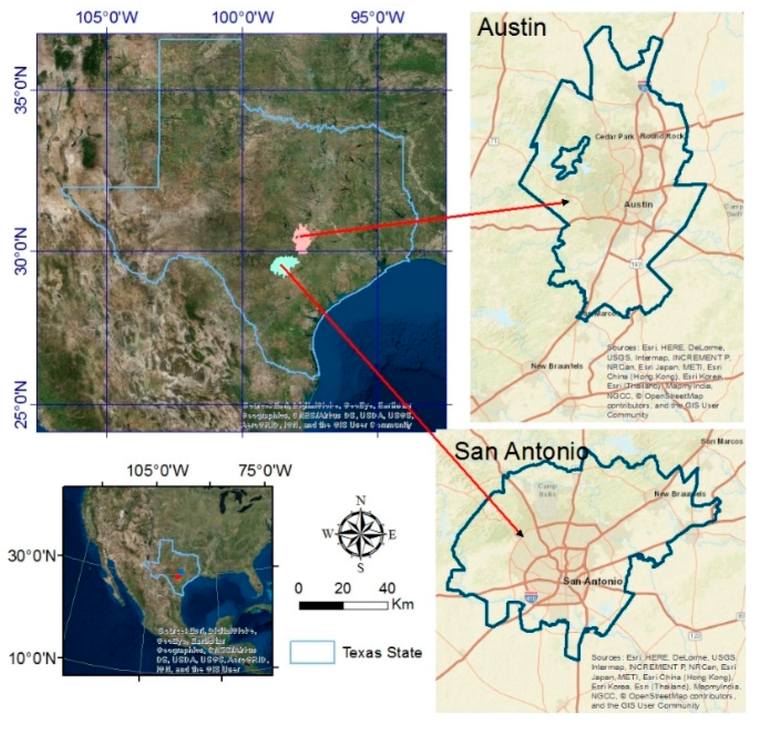
Previous studies have focused on analyzing SUHI for single cities, while SUHI research on broader metropolitan areas of multiple cities is far less common. This larger extent analysis warrants further investigation since the underlying factors are likely to be more complex and variable over space. The Austin and San Antonio metropolitan areas in Texas, USA were selected for our LST mapping because of their hot and humid summers and population concentrations (Figure 1 and Table 1). However, there have been few UHI studies within these two metropolitan areas, and comparisons of UHI results are difficult because of variations in mapping units and land cover characteristics. Under that backdrop, the main objectives of this study are to answer the following questions: (1) Which underlying landscape properties (e.g., land cover and terrain morphology) are significantly related to the SUHI phenomena for Austin and San Antonio, Texas, and (2) compared to a global regression approach, does GWR provide improved insight about the landscape drivers of LST?
2. Materials and Methods
2.1. Study Areas
As two of the four major metropolitan areas of Texas, the Austin–Round Rock (Austin) and the San Antonio–New Braunfels (San Antonio) metropolitan areas are located in the central south region of Texas, USA (Figure 1). The Interstate highway I-35, a major transportation corridor, passes north-south through these two metropolitan areas. Both areas are characterized by relatively flat terrain to the east, grading to more complex topography along the Western edge of the Balcones Escarpment. Based on the Köppen climate classification scheme, the region is considered humid subtropical with long and hot summers, short and mild winters, and warm and rainy spring and fall seasons [34] (Table 1). Both the Austin–Round Rock and San Antonio–New Braunfels metropolitan areas are located in a unique and narrow transitional zone that ranges from semi-arid vegetation cover dominated by trees and shrubs in the west, to humid and more densely vegetated prairie/grassland to the east.
2.2. Data Collection and Preprocessing
2.2.1. Landsat 8 OLI/TIRS Imagery
The moderate spatial resolution and spectral bands of Landsat data are amenable to modeling SUHI variation and underlying landscape patterns at the extent of a metropolitan area. Because of the harmful impact of high temperature on human health in our study areas, summer (June, July, and August) and day-time SUHI phenomena were considered in this SUHI study. Meanwhile, at least two Landsat images are needed to cover the entire San Antonio area. In this sense, two cloud-free Landsat 8 OLI/TIRS images acquired on 20 July 2015 were obtained from the United States Geological Survey (USGS) Earth Explorer for LST calculation and derivation of related spectral indices (e.g., NDVI). Image preprocessing was implemented using ERDAS Imagine 2015 and included stacking individual bands and clipping the image stack of the study areas. Digital numbers for all reflective bands were converted to top-of-atmosphere (TOA) reflectance using scaling coefficients provided in the image metadata.
2.2.2. Lidar Dataset Processing
Lidar data were used to calculate a series of morphological properties closely related to SUHI variation, including topography and building morphology. Lidar datasets were obtained from the Texas Natural Resources Information System (TNRIS) and downloaded using an online interface. Table 2 provides the relevant metadata information about the different airborne Lidar survey project between 2007 and 2012 that were used to calculate the Lidar-derived model covariates. Lidar data processing included the generation of digital terrain models (DTM) and building footprint extraction. Five-meter DTMs were generated using the “LAS Dataset to Raster” tool in ArcGIS 10.5 for individual Lidar projects, using the 3D Analyst Conversion Toolbox and “Average Cell Assignment Type” for ground classified returns. The DTMs from the different source projects were merged together after being re-projected to the same spatial reference (NAD UTM Zone 14N). Similarly, 5 m digital surface models (DSMs) were generated with the same tool but using the “Maximum Cell Assignment Type” for all Lidar returns. The DSMs represented the ground surface combined with built-up areas, vegetation, and other features on the landscape. The same reprojection and data merging procedures were applied to the DSMs. Figure 2 shows the spatial pattern of DSMs for the study areas and a detailed illustration of DSMs for a selected area in San Antonio.
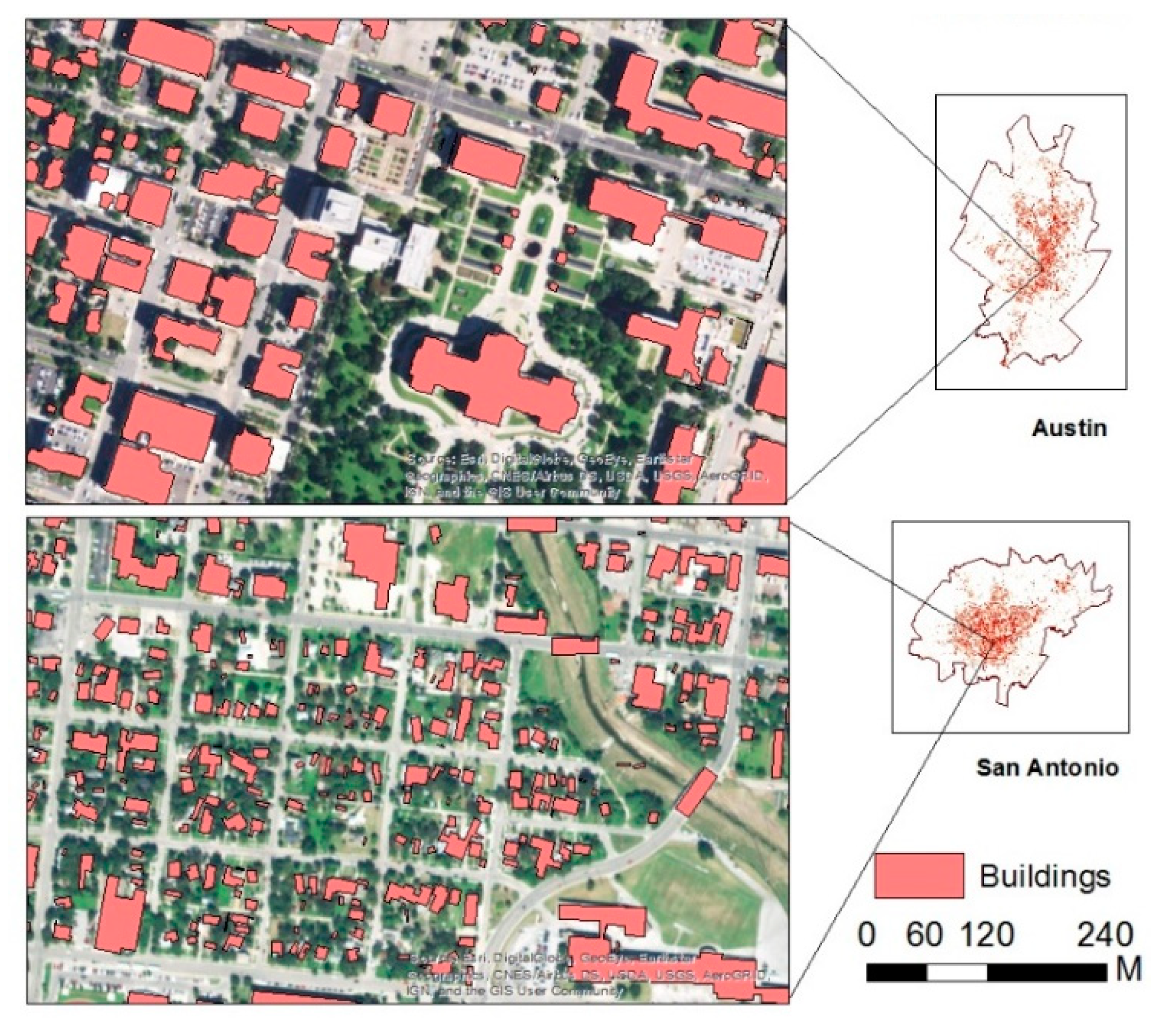
Buildings are an essential component of SUHI formation, both in terms of building height and fractional cover on the landscape. Building footprints for portions of central and south Austin were created by the City of Austin Enterprise Geospatial Services; however, they did not cover the entire metropolitan area. Consequently, we extracted building footprints using the dataset of Lidar points in LP360, a type of software for Lidar data management and post-processing. Buildings were first classified using the point cloud task tool “Planar Point Filter”, in which the parameters were set after several trial and error runs. Subsequently, building outlines were extracted as polygons from the Lidar data in LP360 with the automated point cloud task tool “Point Group Tracing and Squaring” for the developed areas. To further improve the accuracy of the building extraction, we manually interpreted and deleted erroneous building outlines with the aid of high-resolution current and historical images from Google Earth and base maps in ArcGIS. Figure 3 provides examples of detailed building extraction results for selected intensively developed areas.
2.3. SUHI Measurement
Top-of-atmosphere (TOA) radiance (i.e., radiance measured by the sensor) was converted to brightness temperature according to the following formula:
where is the temperature in Kelvin (K), and K1 and K2 are calibration constants specific to the Landsat TIRS sensor which can be obtained from the image metadata.
The brightness temperature was further adjusted using land surface emissivity (LSE) which is essential for LST inversion due to the noteworthy thermal variation of different land surface properties at a large spatial extent. The variation of vegetation coverage, surface moisture, roughness, and viewing angles leads to different LSEs for different cover types [35]. The Normalized Difference Vegetation Index (NDVI) threshold emissivity estimation algorithm [36,37], a common method for LSE estimates, was applied in this study. The NDVI values were used to distinguish between soil and vegetated pixels before LSE calculation. The radiance-corrected values of band 4 (Red) and band 5 (NIR) from Landsat OLI were used for the corresponding NDVI calculation to mitigate the effects of vegetation phenology.
Specifically, following instructive literature, an NDVI threshold for rocks/soil () was assigned a value of 0.2, and the NDVI threshold for vegetation () was assigned a value of 0.5 [23,35]. Thus, any pixel for which NDVI < was assumed to be bare soil or rock with an (emissivity) value of 0.966. If NDVI > , a pixel was considered to be fully vegetated and assigned an value of 0.986 [35]. If the NDVI was between and , then the pixels were considered to be a combination of vegetation and rocks/soil. Equations (2)–(4) were used to represent the relationship between NDVI and LSE to calculate the LSE for corresponding pixels.
is a geometrical factor, assigned a value of 0.55, by assuming different geographical distributions [37], while is the vegetation fraction.
The Planck’s function was used to perform LSE correction of the substance compared to the blackbody. Thus, brightness temperatures were converted to LST [38,39].
2.4. OLS and GWR Analysis
Unlike a conventional (global) regression model, GWR is able to model spatial variation in the relationship between dependent and independent variables. A GWR model takes the following form:
where , , and are the dependent variable, the k independent variable (subscripted as k), and the random error at point i (subscripted as subscript i), respectively. The location is denoted by the coordinates of a given point (i). The coefficients are varying weights on the location, and is the geographically varying intercept. Thus, the GWR extends the global regression model by adding the geographical location parameter to generate the local coefficients to account for spatial non-stationarity. The estimates of and are based on the unbiased estimation of a set of observations, in which the weight matrix is used to weight the observations differently [40]. The variation in at different locations makes the GWR different from the OLS. The distance to the given point (i) is an important factor that affects the weight matrix:
Generally, the Gaussian function is used to generate the weight matrix with the following form:
Here, an adaptive Gaussian kernel function was adopted for the analysis, where optimal the bandwidth was detected through a golden search algorithm in GWR 4. Here, by incorporating the weight into the pooled observations, the GWR yielded more precise estimates compared to the OLS.
Global regression models were also developed and compared to the GWR results. The coefficient of determination (R2), the global Moran’s I of the residuals, the Akaike Information Criterion (AIC), and the corrected AICc were used to compare the performances of global regression models versus the GWR model with respect to the goodness-of-fit and residual spatial autocorrelation. In this paper, both the GWR and global regression models were built using the open source platform GWR 4 [41].
2.5. Derivation and Selection of Explanatory Variables
Based on knowledge from prior SUHI studies [21,22,23,24,25,26,27], a suite of potential explanatory variables was selected for two models, one each for the metropolitan areas under consideration. Considering the variable type, the explanatory variables were categorized into three groups, as summarized in Table 3.
2.5.1. Land Use/Land Cover Composition (LULC) Variables
The Buildings Fraction (BF), Impervious Surfaces Fraction (ISF), NDVI, and Canopy were considered for SUHI explanatory variables in terms of the LULC composition. ISF and Canopy were downloaded as independent layers from National Land Cover Database (NLCD) 2011 [42], the thematic accuracy of which has been established in the literature [43]. BF was derived using the building footprint features based on the Lidar datasets.
2.5.2. Landscape Pattern Metrics
The 30 m NLCD 2011 data was used to compute landscape metrics at the landscape level to quantify the general characteristics of the overall mosaic of LULC patches [42]. The LULC types of the study area included open water, developed land (in four intensity levels), forest (deciduous, evergreen, and mixed), shrub/scrub, grassland/herbaceous, pasture/hay, cultivated land, and wetlands (woody, herbaceous).
The Contagion Index (CONTAG) and Patch Density (PD) were applied to describe aggregation. CONTAG is inversely related to the edge density. For instance, when a single class occupies a very large percentage of the landscape (low edge density), contagion is high and vice versa. It is affected by both the dispersion and interspersion of land types. PD is the number of patches on the landscape and describes the aggregation and subdivision characteristics of the various land covers. The Shannon's Diversity Index (SHDI) considers the proportional abundance of each patch type across all patch types and the Patch Richness (PR) quantifies the number of different patch types. These metrics were selected to measure the diversity characteristics on the landscape. In regard to optimal sampling scale selection, our previous study of Local Climate Zones (LCZs) indicated that 270 m is an optimal scale for an urban climate study as a uniform measure of land cover and surface structure [44]. Based on this finding, 1000 m × 1000 m grids cells were used as observations to mitigate the spatial dependence and spatial autocorrelation. For consistency, all landscape metrics were calculated in FRAGSTATS using a radius of 1000 m centered on sampling points distributed throughout the study areas.
2.5.3. Terrain Factors: Elevation and Northness
Air temperatures are influenced by the elevation [45] and variation in elevation results in spatial patterns of LST on the landscape [30]. Additionally, the landform aspect strongly affects the intensity of solar radiation and has been included in several SUHI studies [30,31]. Aspect (the compass direction of a slope) was transformed to northness to mitigate the circular property of the data using Equation (9):
All of the explanatory variables were aggregated or resampled to a resolution of 90 m to match the dependent variable (LST). Furthermore, to mitigate spatial autocorrelation and to ensure that the sampling dataset represented the study area with sufficient information to understand SUHI patterns, a systematic sampling scheme was designed to obtain sampling points for the regression models. We referred to the previous SUHI explanatory studies at the megacity level and used 1000 m as the sampling interval for further exploration [30]. The center points of the cells which were completely within the boundaries of the study areas were selected as independent observations. Finally, 3887 and 4113 samples were generated for the Austin and San Antonio metropolitans, respectively.
3. Results
3.1. LST Spatial Distribution
The spatial distribution of LSTs revealed the formation of an SUHI on 20 July 2015 for the two metropolitan areas (Figure 4). As expected, extreme values of LST (>35 °C) were often associated with the distribution of major transportation lines (e.g., I 35) and high-density buildings. The high LST (>30 °C) areas for each study area were mainly in both downtown centers and isolated urbanized areas (e.g., Georgetown, New Braunfels). In contrast, low LSTs (<25 °C) were distributed in central to Western Austin and Northern San Antonio, where forested areas and water bodies are located. The remaining areas exhibited relatively cool LSTs.
3.2. Diagnostics of the Regression Models
Prior to modeling, correlation analyses were conducted among the explanatory variables to assess multicollinearity. Variance inflation factors higher than 10 were considered highly correlated. Of the all candidate variables, five were used for analysis in the following global and local regression analysis: the Shannon’s Diversity Index (SHDI), the Buildings Fraction (BF), NDVI, northness, and elevation. For the sake of comparability and interpretation, all of the dependent and independent variables for each were transformed to a range of values spanning from 1 to 100 as the inputs for the global and GWR model.
The global regression models for each of the two study areas estimated statistically significant (p < 0.001) relationships between the LST and all explanatory variables (Table 4). For Austin, the coefficient of determination (R2) for the global regression model was estimated to be 0.53. Among the explanatory variables, the SHDI, BF, and elevation were found to vary positively with LST, while the NDVI and northness were negatively correlated with LST. The global model for San Antonio resulted in an R2 of 0.45 and revealed the same tendencies regarding the explanatory variables and LST with one exception—the relationship between SHDI and LST was not statistically significant in the San Antonio model.
Compared to these global regressions, GWR models seem better suited to the investigation of the SUHI and the underlying influencing factors for both study areas. Specifically, in the case of the Austin metropolitan area, the higher R2 (0.85) for the GWR model suggests that the relationships between LST and the modeled underlying physical factors may exhibit spatial non-stationarity. Such circumstances are one reason why the GWR model seems to outperform the global regressions (Table 4). While the AICc (the corrected Akaike Information Criterion) is not an absolute measurement of goodness of fit, it contributes to the model comparison. Taking the Austin area as an example, the difference between AICc and GWR (e.g., 25,271.62) is much lower (4468.63) than that of the global model, which indicates the benefits of moving from the OLS to the GWR. Additionally, a full comparison of other diagnostic measures further suggests improved performance for GWR compared to the global regression model, including F-tests of GWR model improvement (34.42, Austin), and the Global Moran's I of the residuals (e.g., 0.44 for GWR vs 0.058 for the global model in Austin).
3.3. The Global and Spatial Non-Stationarity Relationship
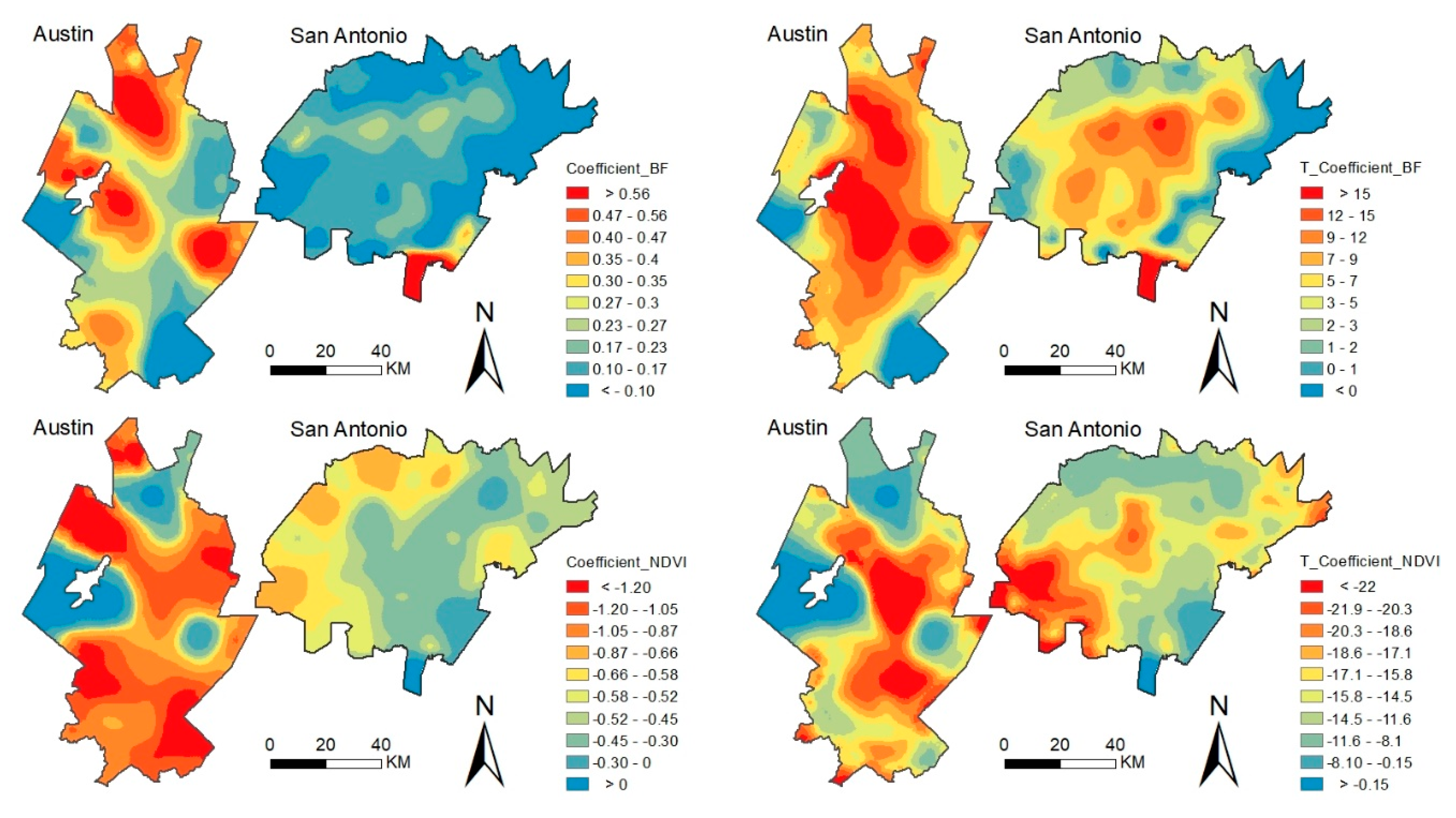
Ordinary kriging interpolation using the Spatial Analyst Toolbox in ArcGIS 10.5 was applied to interpret the samples using a resolution of 300 m for the sake of visualization. First, both the global and GWR analyses indicated that LULC affected the LST variation on 20 July 2015, as indicated by the BF (Buildings Fraction) and NDVI (Table 4). GWR further revealed strong spatial heterogeneity in their relationships based on the coefficient values and t statistics. These covariate relationships were similar for Austin and San Antonio in the same range of estimates of BF coefficients (ranging from 0 to 0.6). Additionally, the t statistics of BF coefficients for both Austin and San Antonio indicated that the relationship between the LST and BF was significant for most of the study areas, especially urban areas. Nevertheless, the effect of BF was more prevalent for Austin than for San Antonio, as evidenced from the higher estimates of BF coefficients indicated by the global and local models. While the highest values of the local estimates of BF coefficients (displayed in red) were located in the isolated natural areas (Figure 5), the effect of the BF was prevalent and most of the high values were distributed in areas with compact human settlements (displayed in yellow and slight blue).
As expected, an increase in NDVI reduced the SUHI effect, as suggested by the significantly negative relationship between LST and NDVI across the study areas. The estimated coefficient from the global regression was −0.74 for Austin and −0.38 for San Antonio, revealing a stronger relationship for LST and NDVI for Austin than San Antonio (Table 4). This fact was further proved by the GWR analysis, the values of local absolute coefficients were higher overall in Austin (e.g., displayed in red for majority of the region) than in San Antonio, indicating a higher capacity to mitigate the SUHI. However, attention should also be paid to the area around the Lake Travis in Austin and nearby the Calaveras Lake in San Antonio, where LST was notably positively related to NDVI, and the relationship was not significant in some part of this area, as indicated by t statistics (Figure 5).
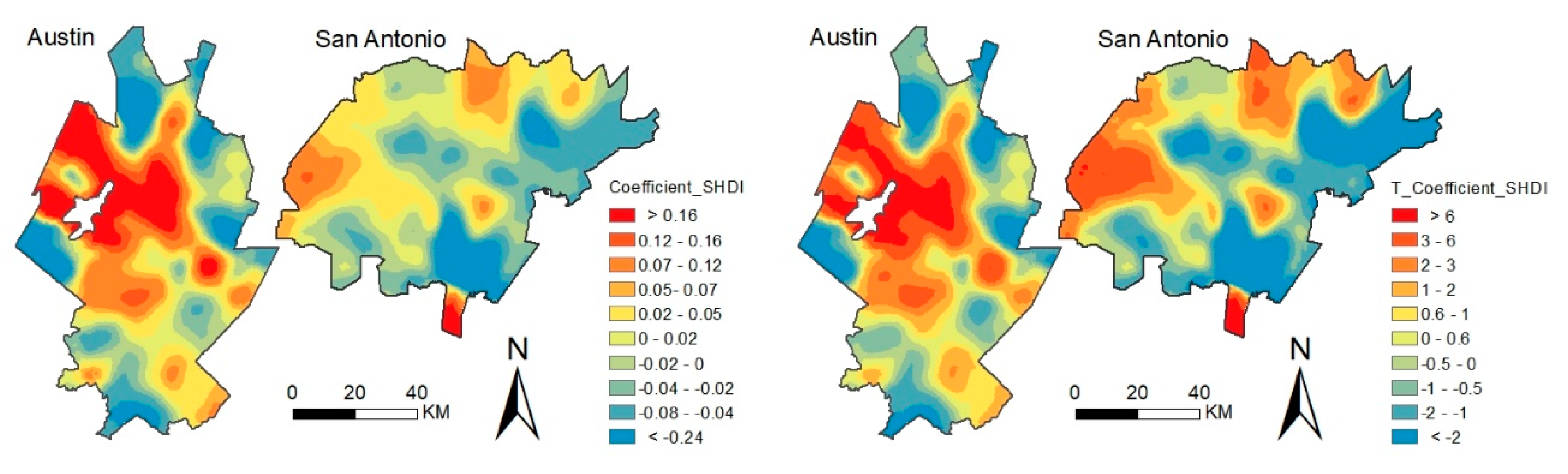
SHDI, as the indicator of the diversity of landscape spatial arrangement, had an overall positive effect on the LST intensity, as explained by the global regression for Austin (Table 4). It indicated that the fragmented landscape (e.g., the interaction of different land patches) would lead to a decrease in the capacity to mitigate SUHI. This effect was further proved by the GWR analysis, from which the regression coefficient was positive for most of the area. However, it is notable that the situation was contrary in the area around the Lake Travis in Austin, as indicated by the slightly negative local regression coefficients (Figure 6). Additionally, the global regression revealed a non-relationship between SHDI and LST for the San Antonio metropolitan area, and GWR further found that the effects of SHDI on LST variation were not significant for most of the area, as indicted by t statistics (e.g., −1.5 to 1.2, Figure 6). Nevertheless, the GWR analysis did find some exceptions where the SHDI was a strong predictor for LST variations (e.g., the small areas in the Southern and Northeastern parts of San Antonio metropolitan area colored in red, Figure 6). By linking with Google Earth imagery and the NLCD 2011, we found that Southern part displayed in red is covered by forest, pasture, and shrub with high complexity. Also, this area demonstrated low DSM, as indicated by Figure 2.
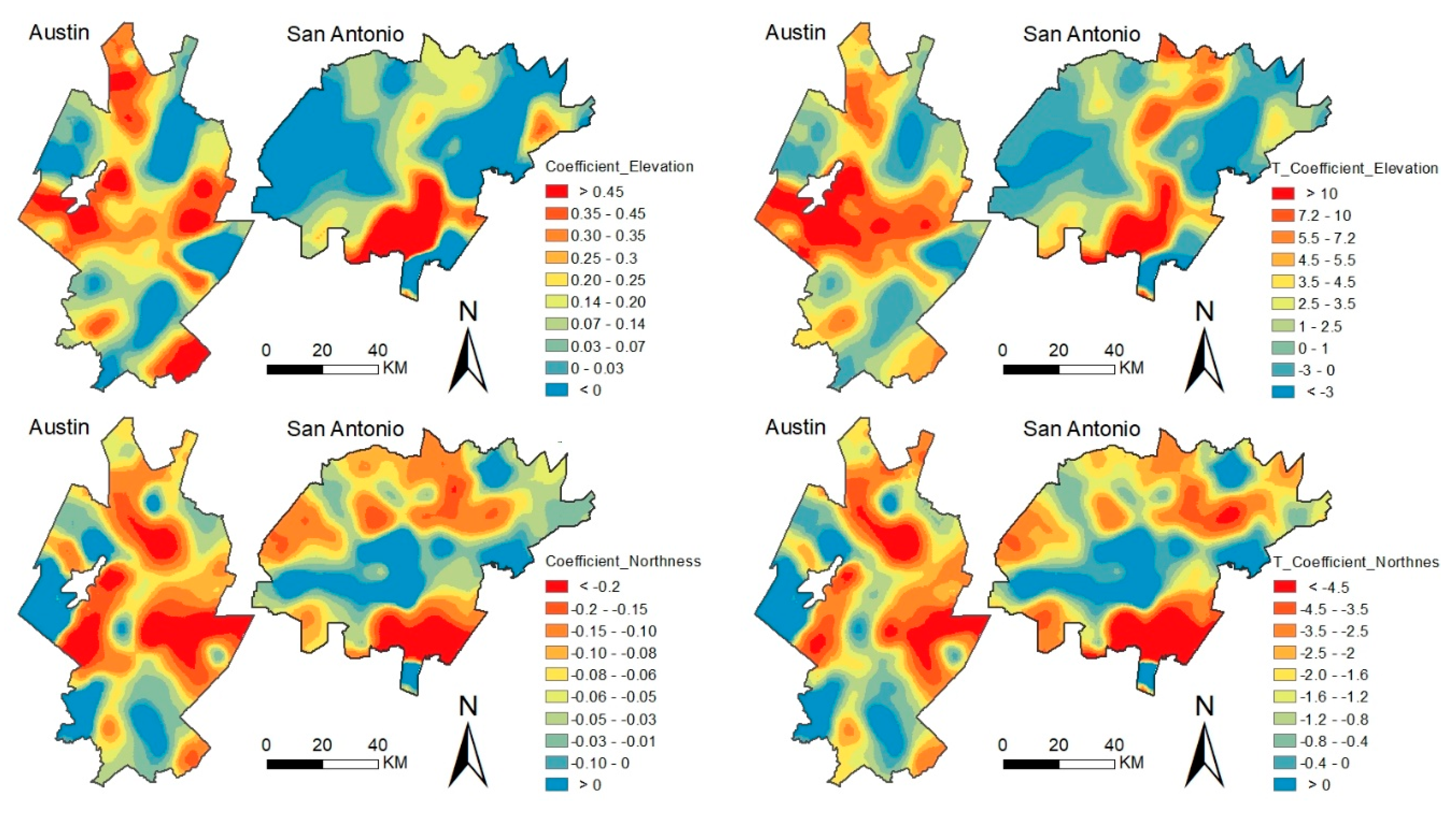
Terrain factors affected the LST variation on 20 July 2015, as indicated by the elevation and northness. For both Austin and San Antonio, the elevation exhibited an overall slight positive effect in the global regression (e.g., 0.20 and 0.09 of coefficients, Table 4). GWR further helped to explore this unexpected finding by indicating that negative coefficients indeed exist in the rural areas for both Austin and San Antonio, especially in the areas with low vegetation cover (e.g., the Northeastern part of Austin and Eastern San Antonio colored with blue, Figure 7). On the other hand, both the global and local regressions yielded the significantly negative coefficient (average coefficient) of northness, which indicated that the northness is a strong predictor of the LST (Table 4). Again, the effect of northness varied spatially, and it had a stronger effect on San Antonio (−5.34 vs. −2.07 indicated by the global regression, Table 4), especially in the Northern part (a larger area colored with red indicated by the GWR, Figure 7).
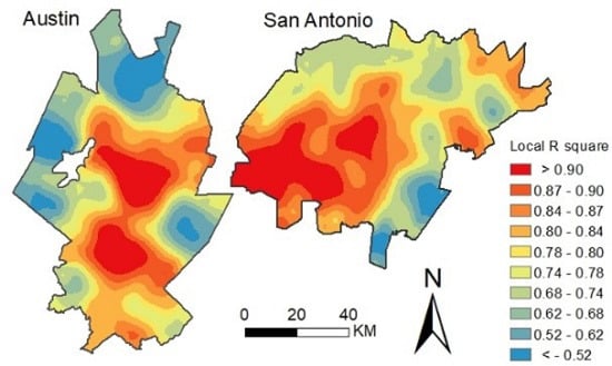
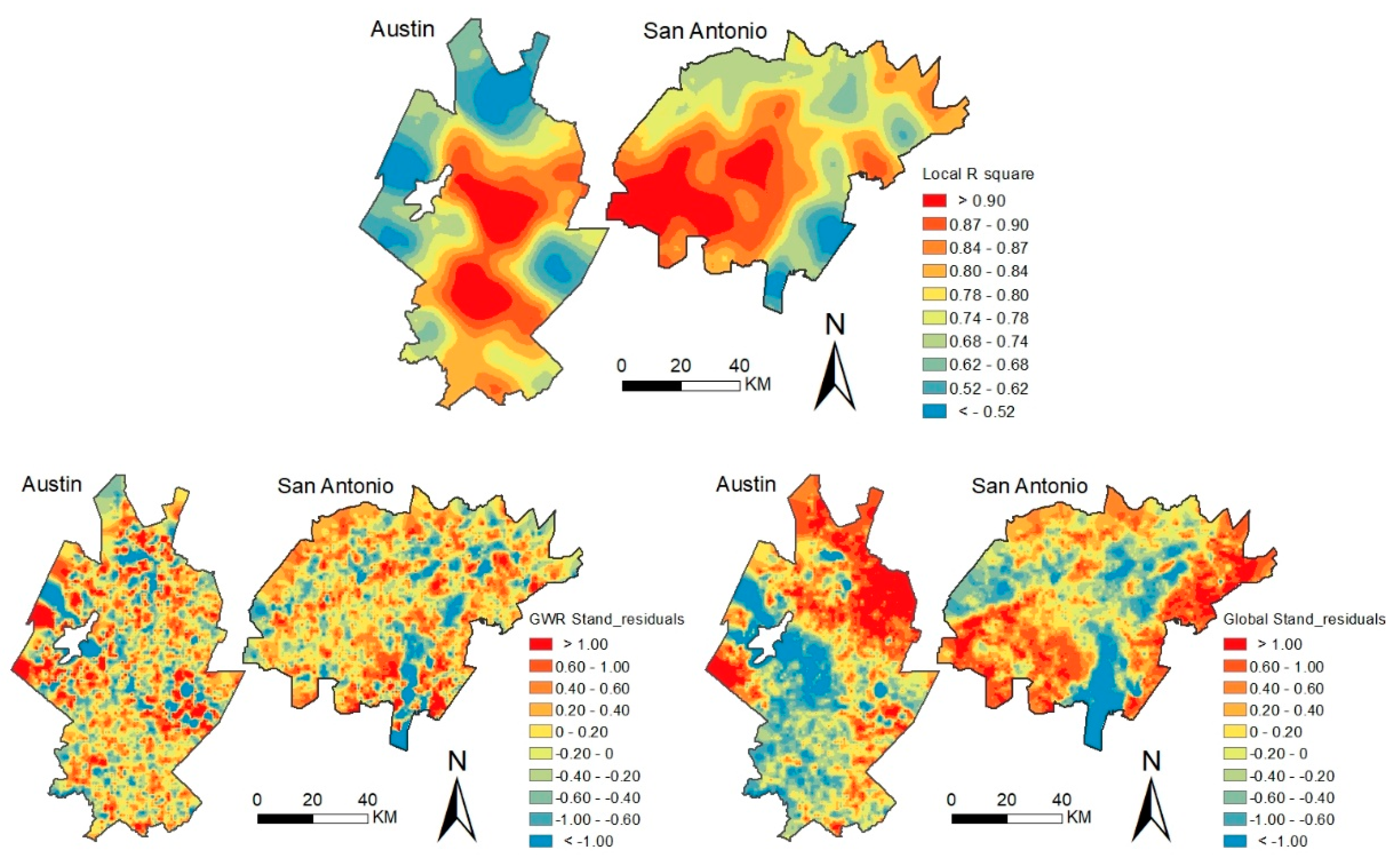
The spatial patterns of the local determination coefficients (R2) of the GWR model highlighted a marked regional heterogeneity. Overall, GWR outperformed the global regression with local R2 values larger than 0.5 across both study areas (Figure 8). GWR modeling was also characterized by higher local R2 values in the city centers (>0.8) while relatively lower values were observed (0.5–0.65) in the surrounding areas. Standardized residuals, indicating the under or overprediction of LST, were distributed with significant spatial autocorrelation as tested by the Global Moran’s I test in ArcGIS. As shown in Figure 8, the standardized residuals from both global and local regression were distributed in clusters, while the spatial clustering effect resulting from the global regressions was much more apparent than those resulting from the GWR.
4. Discussion
4.1. Which Underlying Properties Are Significantly Related to the SUHI for Austin and San Antonio?
Overall, the regression analyses revealed that LULC composition and terrain morphology are closely related to SUHI effects for both metropolitan areas. Similarities in climate and topography for these metropolitan areas facilitates the comparison of their respective SUHIs. First, the composition of land cover was shown to be an essential factor that influences the LST pattern for both study areas. Our study confirmed previous findings that an increase in the building density (e.g., Buildings Fraction; BF) tends to exacerbate the SUHI effect, while an increase in the vegetation cover intensity tends to mitigate the SUHI effect [24,33,46,47,48,49]. Regarding the regional differences, although the effects tended to be similar, building density and vegetation cover intensity were more strongly correlated with the SUHI phenomenon in San Antonio than in Austin, as indicated by global BF coefficient (0.29 vs. 0.19) and NDVI coefficient (−0.74 vs. −0.38) (Table 4). Furthermore, it is notable that the situation was contrary in the area near a water body (e.g., Lake Travis in Austin) as indicated by the slightly negative local regression coefficients. The unique characteristics of water bodies regarding thermal characteristics were also consistent with previous studies [17,47].
Both global and local regressions provided unexpected results for elevation. Our results show that an increase in elevation is associated with an overall increase of LST. It is different with the common knowledge that air temperature decreases with an increase in altitude. In fact, it was DTM (e.g., bare earth digital terrain model) that was used as the potential explanatory factor for LST variation, while the actual surface temperature of the property was being remotely sensed. Air temperature varies between about 0.6 and 1.0 K per 100 m elevation change. Given its small variation in the study area, the effect of elevation may not be substantial. Thus, in the areas with dense building or forest cover, the effect of elevation would be not as severe as other factors when incorporating them simultaneously in the modeling. Also, most areas of Austin and San Antonio exhibit flat terrains; thus, the effect of elevation was not apparent. Furthermore, the Lidar-derived DSM proved to be an effective way to characterize the terrain morphology at the microscale (e.g., 5 m × 5 m) to understand the relationship between northness and SUHI variation. Consistent with previous studies, this research indicated that the alleviating effect of northness was more apparent for floodplain areas with low and flat terrains for both the Austin and San Antonio metropolitan areas (e.g., Refs. [31,32,33]).
The effect of landscape configuration on SUHI formulation has drawn attention in recent years by incorporating the landscape matrix at the patch, class, or landscape level [21,22,23,26,27,46]. For example, a recent study by Kim, et al. [50] found that larger and better-connected landscape patches have the effect of mitigating high LST at the neighborhood scale, while fragmented and isolated patches showed the opposite effect in the city of Austin. Similarly, this study found that the SUHI of Austin on 20 July 2015 was also affected by the spatial pattern of LULC, measured by SHDI, which was not detected in San Antonio.
These contrasting findings may be explained by the fact that the landscape of San Antonio is more aggregated and less diverse as indicated by the statistics of potential explanatory variables (Table 3). In this study, to balance the spatially detailed characterization of SUHI and the size of samples in the modeling, 1000 m was set as the sampling interval as well as the window size for landscape matrix calculation for both study areas. Since both landscape patterns and LST distributions are scale dependent, previous studies have drawn different conclusions on the suitable scale for investigation of the relationship (e.g., 700 m for Beijing, China [51]; 600 m for Wuhan, China [52]). In addition, the appropriate scale also depends on landscape matrix selection. For instance, the SHDI showed the strongest correlation with LST at the 700 m scale which was not the optimal solution if other landscape matrices were taken into account, as indicated by a case study of Wuhan, China [53]. In this sense, further research is warranted to examine the scale sensitivity of their relationships in the future to lead to more comprehensive understanding.
4.2. Compared to the Conventional Regression Model, Does the GWR Provide Fresh Insight into the SUHI Phenomenon?
As a natural process, SUHI exhibits high spatial heterogeneity which is difficult to characterize with conventional regression methods. However, most previous studies derived the spatial relationship by focusing on individual cities, especially for cities in Asia [24,33,46,47,48,49], while varying heterogeneous impacts have been rarely studied and compared. The results reported in this paper suggest significant spatial non-stationarity in the relationship between the LST and explanatory variables for the two metropolitan areas. Here, GWR modeling was confirmed as an effective method to detect non-stationarity, especially for the urban cores of Austin and San Antonio as well as Western San Antonio with local R2 values of higher than 0.8.
Furthermore, locally detailed differentiation of the underlying mechanisms of SUHI provided by non-stationarity GWR modeling is necessary for partitioned regional landscape planning. With the implementation of GWR, studies have suggested site-specific policies designed for effective SUHI mitigation, including land use planning that considers the distance to roads to alleviate the high LST effect [30] and the location and configuration of green spaces in urban areas [31]. Considering natural and socioeconomic factors, Li, Cao, Lang and Wu [33] mapped the potential heat sources and sinks of a megacity and performed GWR analysis based on the heat source and sink regions, where the partitioned policies were provided.
Whereas a classic regression method would provide an estimate of the mean value for an entire region regardless of the spatial pattern, GWR can infer a more dynamic approach to parameter estimations by using data from neighborhoods to determine the model parameters. In the case of identifying whether the SUHI phenomenon is influenced by local underlying physical factors, this dynamic model approach is desirable, as a “one size fits all” approach may not accurately identify the LST variation across a heterogeneous metropolitan landscape. In short, compared to conventional regression, GWR has the inherent potential to enable a better understanding of SUHI phenomenon and associated biophysical factors across the metropolitan area.
5. Conclusions
In this study, we used Landsat imagery from 20 July 2015, a Lidar dataset and derived products, NLCD 2011 land cover, and associated fractional cover products as the main data sources to investigate SUHI spatial distribution in the Austin and San Antonio metropolitan areas. This study further explored how the underlying surface characteristics affect SUHI phenomenon by using global regression and GWR analysis.
The results indicate that the GWR is in overall agreement with the global regression, and that both help to address the contributions of a set of specific underlying physical factors related to the SUHI phenomenon. The composition of land cover is an essential factor that influences the LST pattern for both study areas. Furthermore, the Lidar-derived DSM was proved to be an effective way to characterize the terrain morphology at the microscale (e.g., 5 m × 5 m) to aid in the understanding of the relationship between northness and SUHI variation. This study further found that the SUHI of Austin on 20 July 2015 was also affected by the spatial pattern of LULC, measured by SHDI, which was not detected in the San Antonio metropolitan area. Overall, this study contributed to obtaining a better understanding of SUHI phenomenon.
By accommodating spatial non-stationarity and allowing the model parameters to vary in space, GWR illustrated the spatial heterogeneity of the relationship between different land surface properties and the LST. In particular, the GWR analysis revealed considerably stronger relationships in some areas. Thus, together with the mapping result, the GWR analysis of the SUHI phenomenon can provide unique information for site-specific land planning and policy implementation for SUHI mitigation.
In this paper, the LST was calculated from a Landsat sensor, and the effect of urban facets was not considered in this SUHI study. For instance, in a dense built-up neighborhood, the uneven solar heating on different building surfaces can lead to the anisotropy of surface thermal emission [54,55]. The LST on 20 July 2015 was calculated as the dependent variable, while the variation in the SUHI pattern at different times may affect the regression result. Uncertainties also come from the inconstancy of the acquisition time among input and output data for modeling. NLCD was built in the year 2011, whereas Lidar projects were conducted by different agencies with different accuracy standards and different time periods (Table 2). Hence, further work on the complete surface temperature acquisition and SUHI spatiotemporal variation is warranted. Then, a robust analysis of underlying properties related to the SUHI phenomenon can be performed.
Author Contributions
Conceptualization, C.Z.; Data curation, C.Z.; Formal analysis, C.Z. and R.W.; Funding acquisition, J.J.; Investigation, C.Z.; Methodology, C.Z.; Project administration, J.J.; Resources, J.J.; Software, J.J.; Supervision, J.J. and Q.W.; Validation, Q.W. and R.W.; Visualization, J.J.; Writing, review & editing, Q.W. and R.W.; Final check and submission, Q.W.
Acknowledgments
A special thank you goes to the assistant from the Texas Natural Resources Information System (TNRIS), who shared the Lidar point data in an efficient way. Appreciation also goes to Nathan Currit from Texas State University, who provided essential feedback and suggestions that significantly improved the manuscript.
Conflicts of Interest
The authors declare no conflict of interest.
References
- Lambin, E.F.; Turner, B.L.; Geist, H.J.; Agbola, S.B.; Angelsen, A.; Bruce, J.W.; Coomes, O.T.; Dirzo, R.; Fischer, G.; Folke, C. The causes of land-use and land-cover change: Moving beyond the myths. Glob. Environ. Chang. 2001, 11, 261–269. [Google Scholar] [CrossRef]
- Liu, Z.; He, C.; Zhou, Y.; Wu, J. How much of the world’s land has been urbanized, really? A hierarchical framework for avoiding confusion. Landsc. Ecol. 2014, 29, 763–771. [Google Scholar] [CrossRef]
- United Nations. World Urbanization Prospects: The 2014 Revision. Erscheinungsort Nicht Ermittelbar United Nations s.l.; United Nations: New York, NY, USA, 2014; Available online: http://www.worldcat.org/title/world-urbanization-prospects-the-2014-revision-highlights/oclc/993940509 (accessed on 28 August 2018).
- Chen, Y.-C.; Chiu, H.-W.; Su, Y.-F.; Wu, Y.-C.; Cheng, K.-S. Does urbanization increase diurnal land surface temperature variation? Evidence and implications. Landsc. Urban Plan. 2017, 157, 247–258. [Google Scholar] [CrossRef]
- Oliveira, E.; Tobias, S.; Hersperger, A. Can strategic spatial planning contribute to land degradation reduction in urban regions? State of the art and future research. Sustainability 2018, 10, 949. [Google Scholar] [CrossRef]
- Zhao, C.; Jensen, J.; Zhan, B. A comparison of urban growth and their influencing factors of two border cities: Laredo in the US and Nuevo Laredo in Mexico. Appl. Geogr. 2017, 79, 223–234. [Google Scholar] [CrossRef]
- Hersperger, A.M.; Oliveira, E.; Pagliarin, S.; Palka, G.; Verburg, P.; Bolliger, J.; Grădinaru, S. Urban land-use change: The role of strategic spatial planning. Glob. Environ. Chang. 2018, 51, 32–42. [Google Scholar] [CrossRef]
- Howard, L. The Climate of London: Deduced from Meteorological Observations, Made at Different Places in The Neighbourhood of the Metropolis: 1818; Volume. 1. Available online: https://archive.org/details/climatelondon00howagoog (accessed on 6 September 2018).
- Zhou, D.; Zhao, S.; Zhang, L.; Liu, S. Remotely sensed assessment of urbanization effects on vegetation phenology in China’s 32 major cities. Remote Sens. Environ. 2016, 176, 272–281. [Google Scholar] [CrossRef]
- Sarrat, C.; Lemonsu, A.; Masson, V.; Guedalia, D. Impact of urban heat island on regional atmospheric pollution. Atmos. Environ. 2006, 40, 1743–1758. [Google Scholar] [CrossRef]
- Taha, H. Urban climates and heat islands: Albedo, evapotranspiration, and anthropogenic heat. Energy Build. 1997, 25, 99–103. [Google Scholar] [CrossRef]
- Huang, Q.; Lu, Y. The effect of urban heat island on climate warming in the Yangtze river delta urban agglomeration in china. Int. J. Environ. Res. Public Health 2015, 12, 8773–8789. [Google Scholar] [CrossRef] [PubMed]
- Harlan, S.L.; Brazel, A.J.; Jenerette, G.D.; Jones, N.S.; Larsen, L.; Prashad, L.; Stefanov, W.L. In the shade of affluence: The inequitable distribution of the urban heat island. Res. Soc. Prob. Public Policy 2007, 15, 173–202. [Google Scholar]
- Nichol, J.E. High-resolution surface temperature patterns related to urban morphology in a tropical city: A satellite-based study. J. Appl. Meteorol. 1996, 35, 135–146. [Google Scholar] [CrossRef]
- Weng, Q. Thermal infrared remote sensing for urban climate and environmental studies: Methods, applications, and trends. ISPRS J. Photogramm. Remote Sens. 2009, 64, 335–344. [Google Scholar] [CrossRef]
- Buyantuyev, A.; Wu, J. Urban heat islands and landscape heterogeneity: Linking spatiotemporal variations in surface temperatures to land-cover and socioeconomic patterns. Landsc. Ecol. 2009, 25, 17–33. [Google Scholar] [CrossRef]
- Weng, Q.; Lu, D.; Schubring, J. Estimation of land surface temperature–vegetation abundance relationship for urban heat island studies. Remote Sens. Environ. 2004, 89, 467–483. [Google Scholar] [CrossRef]
- Chen, X.-L.; Zhao, H.-M.; Li, P.-X.; Yin, Z.-Y. Remote sensing image-based analysis of the relationship between urban heat island and land use/cover changes. Remote Sens. Environ. 2006, 104, 133–146. [Google Scholar] [CrossRef]
- Jiang, Y.; Fu, P.; Weng, Q. Assessing the impacts of urbanization-associated land use/cover change on land surface temperature and surface moisture: A case study in the midwestern United States. Remote Sens. 2015, 7, 4880–4898. [Google Scholar] [CrossRef]
- Connors, J.P.; Galletti, C.S.; Chow, W.T. Landscape configuration and urban heat island effects: Assessing the relationship between landscape characteristics and land surface temperature in phoenix, Arizona. Landsc. Ecol. 2013, 28, 271–283. [Google Scholar] [CrossRef]
- Li, X.; Zhou, W.; Ouyang, Z.; Xu, W.; Zheng, H. Spatial pattern of greenspace affects land surface temperature: Evidence from the heavily urbanized Beijing metropolitan area, china. Landsc. Ecol. 2012, 27, 887–898. [Google Scholar] [CrossRef]
- Zhou, W.; Huang, G.; Cadenasso, M.L. Does spatial configuration matter? Understanding the effects of land cover pattern on land surface temperature in urban landscapes. Landsc. Urban Plan. 2011, 102, 54–63. [Google Scholar] [CrossRef]
- Peng, J.; Xie, P.; Liu, Y.; Ma, J. Urban thermal environment dynamics and associated landscape pattern factors: A case study in the Beijing metropolitan region. Remote Sens. Environ. 2016, 173, 145–155. [Google Scholar] [CrossRef]
- Guo, G.; Wu, Z.; Xiao, R.; Chen, Y.; Liu, X.; Zhang, X. Impacts of urban biophysical composition on land surface temperature in urban heat island clusters. Landsc. Urban Plan. 2015, 135, 1–10. [Google Scholar] [CrossRef]
- Xian, G.; Crane, M. An analysis of urban thermal characteristics and associated land cover in Tampa bay and Las Vegas using landsat satellite data. Remote Sens. Environ. 2006, 104, 147–156. [Google Scholar] [CrossRef]
- Zheng, B.; Myint, S.W.; Fan, C. Spatial configuration of anthropogenic land cover impacts on urban warming. Landsc. Urban Plan. 2014, 130, 104–111. [Google Scholar] [CrossRef]
- Myint, S.W.; Zheng, B.; Talen, E.; Fan, C.; Kaplan, S.; Middel, A.; Smith, M.; Huang, H.-P.; Brazel, A. Does the spatial arrangement of urban landscape matter? Examples of urban warming and cooling in phoenix and Las Vegas. Ecosyst. Health Sustain. 2015, 1, 1–15. [Google Scholar] [CrossRef]
- Deilami, K.; Kamruzzaman, M.; Hayes, J. Correlation or causality between land cover patterns and the urban heat island effect? Evidence from Brisbane, Australia. Remote Sens. 2016, 8, 716. [Google Scholar] [CrossRef]
- Fan, C.; Rey, S.J.; Myint, S.W. Spatially filtered ridge regression (sfrr): A regression framework to understanding impacts of land cover patterns on urban climate. Trans. GIS 2017, 21, 862–879. [Google Scholar] [CrossRef]
- Li, S.; Zhao, Z.; Miaomiao, X.; Wang, Y. Investigating spatial non-stationary and scale-dependent relationships between urban surface temperature and environmental factors using geographically weighted regression. Environ. Model. Softw. 2010, 25, 1789–1800. [Google Scholar] [CrossRef]
- Ivajnšič, D.; Kaligarič, M.; Žiberna, I. Geographically weighted regression of the urban heat island of a small city. Appl. Geogr. 2014, 53, 341–353. [Google Scholar] [CrossRef]
- Luo, X.; Peng, Y. Scale effects of the relationships between urban heat islands and impact factors based on a geographically-weighted regression model. Remote Sens. 2016, 8, 760. [Google Scholar] [CrossRef]
- Li, W.; Cao, Q.; Lang, K.; Wu, J. Linking potential heat source and sink to urban heat island: Heterogeneous effects of landscape pattern on land surface temperature. Sci. Total Environ. 2017, 586, 457–465. [Google Scholar] [CrossRef] [PubMed]
- Peel, M.C.; Finlayson, B.L.; McMahon, T.A. Updated world map of the Köppen-Geiger climate classification. Hydrol. Earth Syst. Sci. 2007, 11, 1633–1644. [Google Scholar] [CrossRef]
- Yu, X.; Guo, X.; Wu, Z. Land surface temperature retrieval from landsat 8 tirs—Comparison between radiative transfer equation-based method, split window algorithm and single channel method. Remote Sens. 2014, 6, 9829–9852. [Google Scholar] [CrossRef]
- Sobrino, J.A.; Jiménez-Muñoz, J.C.; Paolini, L. Land surface temperature retrieval from landsat tm 5. Remote Sens. Environ. 2004, 90, 434–440. [Google Scholar] [CrossRef]
- Sobrino, J.A.; Caselles, V.; Becker, F. Significance of the remotely sensed thermal infrared measurements obtained over a citrus orchard. ISPRS J. Photogramm. Remote Sens. 1990, 44, 343–354. [Google Scholar] [CrossRef]
- Artis, D.A.; Carnahan, W.H. Survey of emissivity variability in thermography of urban areas. Remote Sens. Environ. 1982, 12, 313–329. [Google Scholar] [CrossRef]
- Isaya Ndossi, M.; Avdan, U. Application of open source coding technologies in the production of land surface temperature (lst) maps from landsat: A pyqgis plugin. Remote Sens. 2016, 8, 413. [Google Scholar] [CrossRef]
- Guo, L.; Ma, Z.; Zhang, L. Comparison of bandwidth selection in application of geographically weighted regression: A case study. Can. J. For. Res. 2008, 38, 2526–2534. [Google Scholar] [CrossRef]
- Nakaya, T. Geographically weighted generalised linear modelling. In Geocomputation: A Practical Primer; Chris, B., Alex, S., Eds.; Sage Publication: Thousand Oaks, CA, USA, 2015; pp. 217–220. [Google Scholar]
- Homer, C.; Dewitz, J.; Yang, L.; Jin, S.; Danielson, P.; Xian, G.; Coulston, J.; Herold, N.; Wickham, J.; Megown, K. Completion of the 2011 national land cover database for the conterminous united states–representing a decade of land cover change information. Photogramm. Eng. Remote Sens. 2015, 81, 345–354. [Google Scholar]
- Wickham, J.; Stehman, S.V.; Gass, L.; Dewitz, J.A.; Sorenson, D.G.; Granneman, B.J.; Poss, R.V.; Baer, L.A. Thematic accuracy assessment of the 2011 national land cover database (nlcd). Remote Sens. Environ. 2017, 191, 328–341. [Google Scholar] [CrossRef]
- Zhao, C.; Jensen, J.; Weng, Q.; Currit, N.; Weaver, R. Application of airborne remote sensing data on mapping Local Climate Zones: cases of three metropolitan areas of Texas, U.S. Comput. Environ. Urban Syst. 2018. under review. [Google Scholar]
- Khandelwal, S.; Goyal, R.; Kaul, N.; Mathew, A. Assessment of land surface temperature variation due to change in elevation of area surrounding Jaipur, India. Egypt. J. Remote Sens. Space Sci. 2017, 21, 87–94. [Google Scholar] [CrossRef]
- Li, J.; Song, C.; Cao, L.; Zhu, F.; Meng, X.; Wu, J. Impacts of landscape structure on surface urban heat islands: A case study of Shanghai, China. Remote Sens. Environ. 2011, 115, 3249–3263. [Google Scholar] [CrossRef]
- Yue, W.; Xu, J.; Tan, W.; Xu, L. The relationship between land surface temperature and ndvi with remote sensing: Application to shanghai landsat 7 etm+ data. Int. J. Remote Sens. 2007, 28, 3205–3226. [Google Scholar] [CrossRef]
- Estoque, R.C.; Murayama, Y.; Myint, S.W. Effects of landscape composition and pattern on land surface temperature: An urban heat island study in the megacities of southeast Asia. Sci. Total Environ. 2017, 577, 349–359. [Google Scholar] [CrossRef] [PubMed]
- Du, S.; Xiong, Z.; Wang, Y.-C.; Guo, L. Quantifying the multilevel effects of landscape composition and configuration on land surface temperature. Remote Sens. Environ. 2016, 178, 84–92. [Google Scholar] [CrossRef]
- Kim, J.H.; Gu, D.; Sohn, W.; Kil, S.H.; Kim, H.; Lee, D.K. Neighborhood landscape spatial patterns and land surface temperature: An empirical study on single-family residential areas in Austin, Texas. Int. J. Environ. Res. Public Health 2016, 13, 880. [Google Scholar] [CrossRef] [PubMed]
- Song, J.; Du, S.; Feng, X.; Guo, L. The relationships between landscape compositions and land surface temperature: Quantifying their resolution sensitivity with spatial regression models. Landsc. Urban Plan. 2014, 123, 145–157. [Google Scholar] [CrossRef]
- Wang, J.; Qingming, Z.; Guo, H.; Jin, Z. Characterizing the spatial dynamics of land surface temperature–impervious surface fraction relationship. Int. J. Appl. Earth Obs. Geoinf. 2016, 45, 55–65. [Google Scholar] [CrossRef]
- Wang, Y.; Zhan, Q.; Ouyang, W. Impact of urban climate landscape patterns on land surface temperature in wuhan, china. Sustainability 2017, 9, 1700. [Google Scholar] [CrossRef]
- Krayenhoff, E.S.; Voogt, J.A. Daytime thermal anisotropy of urban neighbourhoods: Morphological causation. Remote Sens. 2016, 8, 108. [Google Scholar] [CrossRef]
- Lagouarde, J.-P.; Hénon, A.; Kurz, B.; Moreau, P.; Irvine, M.; Voogt, J.; Mestayer, P. Modelling daytime thermal infrared directional anisotropy over Toulouse city centre. Remote Sens. Environ. 2010, 114, 87–105. [Google Scholar] [CrossRef]
Figure 1.
The Austin and San Antonio metropolitan areas in Texas, U.S.

Figure 2.
Digital surface models (DSMs) with a 5 m resolution for Austin (left), San Antonio (middle), and a detailed illustration of DSMs for a selected area of San Antonio (right).
Figure 2.
Digital surface models (DSMs) with a 5 m resolution for Austin (left), San Antonio (middle), and a detailed illustration of DSMs for a selected area of San Antonio (right).
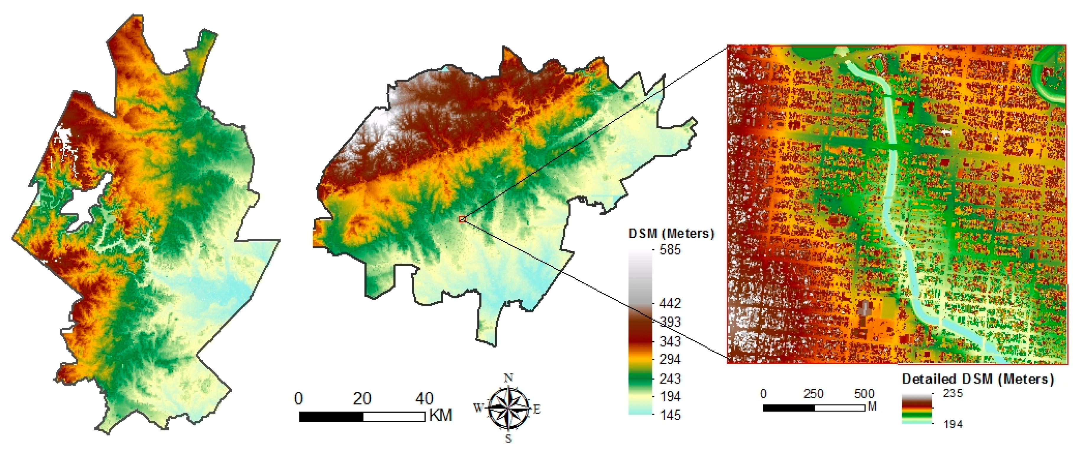
Figure 3.
Detailed illustrations (left) of building extractions from a selected part (right) of the study areas.
Figure 3.
Detailed illustrations (left) of building extractions from a selected part (right) of the study areas.

Figure 4.
Overall spatial variation of the and surface temperature (LST) for the SUHIs of Austin (left) and San Antonio (right) metropolitan areas on 20 July 2015.
Figure 4.
Overall spatial variation of the and surface temperature (LST) for the SUHIs of Austin (left) and San Antonio (right) metropolitan areas on 20 July 2015.
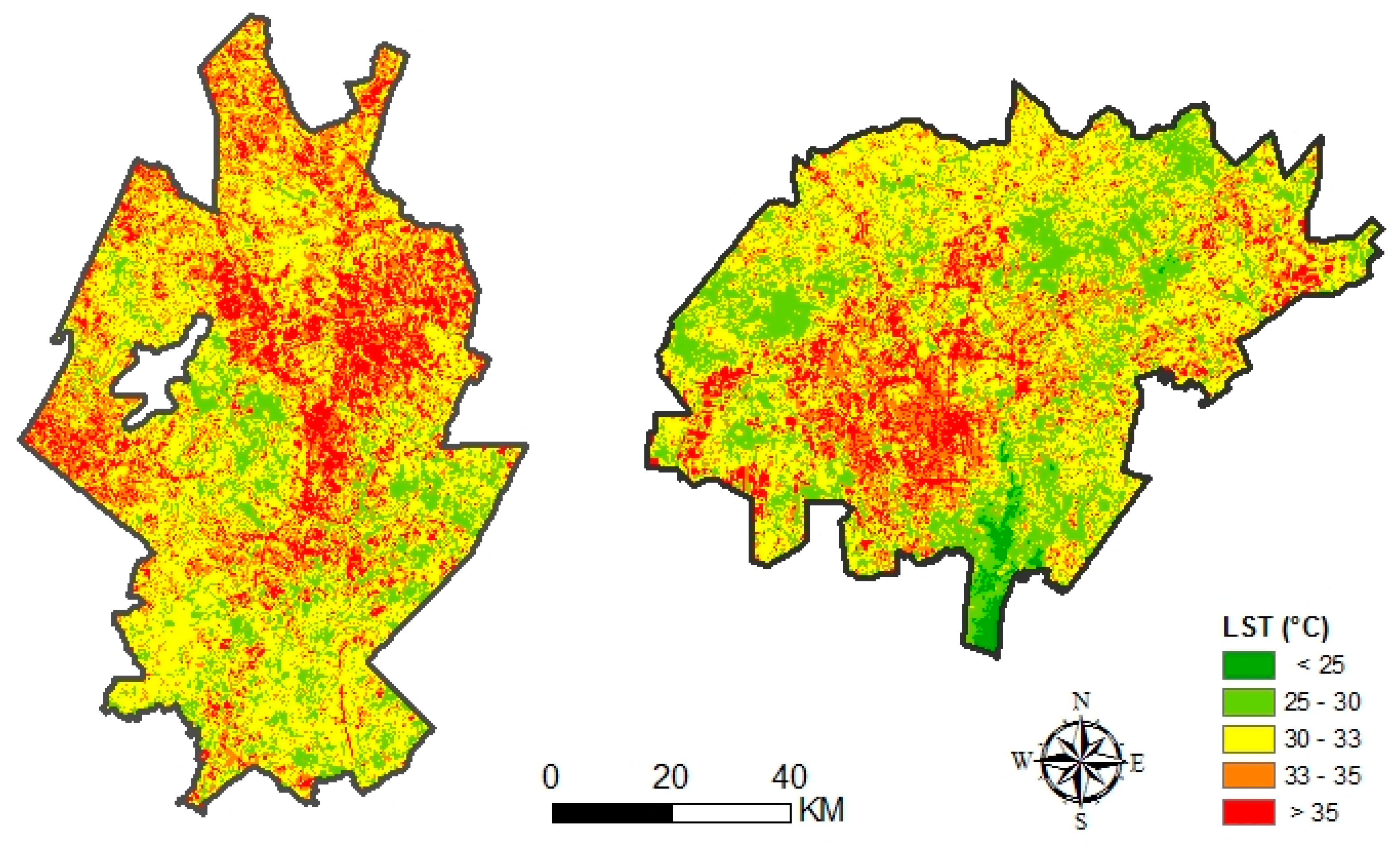
Figure 5.
Overall spatial variation of the coefficients (left) and the t statistics (right): Buildings Fraction (BF) and NDVI.
Figure 5.
Overall spatial variation of the coefficients (left) and the t statistics (right): Buildings Fraction (BF) and NDVI.

Figure 6.
Overall spatial variation of the coefficients (left) and the t statistics (right): Shannon's Diversity Index (SHDI).
Figure 6.
Overall spatial variation of the coefficients (left) and the t statistics (right): Shannon's Diversity Index (SHDI).

Figure 7.
Overall spatial variation of the terrain-related coefficients (left) and the t statistics (right): elevation and northness.
Figure 7.
Overall spatial variation of the terrain-related coefficients (left) and the t statistics (right): elevation and northness.

Figure 8.
Overall spatial distribution of local R2 values (top), standardized residuals of the GWR (bottom left), and global regression (bottom right) as measures of model goodness-of-fit.
Figure 8.
Overall spatial distribution of local R2 values (top), standardized residuals of the GWR (bottom left), and global regression (bottom right) as measures of model goodness-of-fit.


Table 1.
Summary of the geographic, demographic, and climatic characteristics of Austin and San Antonio, Texas.
Table 1.
Summary of the geographic, demographic, and climatic characteristics of Austin and San Antonio, Texas.
| Areas | Location (the Center Point) 1 | Land Area (Square km2) 1 | Estimated Population (1 July 2015) 2 | Bare Earth Elevation (Approximate, meters) 3 | Average Temperature Range (°C), July 4 | Average Precipitation (mm), July 4 |
|---|---|---|---|---|---|---|
| Austin | 30.36°N, 97.78°W | 4587.36 | 931,830 | (107, 405) Mean: 235 | (23.6, 35.3) | 48 |
| San Antonio | 32.76°N, 96.97°W | 4752.04 | 1,469,845 | (116, 579) Mean: 263 | (23.3, 34.8) | 52 |
Sources: (1) Inquired or calculated by the authors in ArcMap based on the projection system “WGS 1984 UTM Zone 14N”. (2) US Census Bureau. (3) Derived from 5 m Digital Terrain Models (DTMs), built by the authors from Lidar data provided by the Texas Natural Resources Information System (TNRIS). (4) US climate data website (www.usclimatedata.com).
Table 2.
Metadata of Lidar projects for the study areas.
| Projects | Point Space and MSE Accuracy (Horizontal/Vertical, cm) | Datum (Horizontal/Vertical) and Projection | Point Classes |
|---|---|---|---|
| CAPCOG 2007 Caldwell, Travis, Williamson | 140; 100/18.5 | NAD83/NAVD88; State Plane Texas Central | Ground/unclassified |
| CAPCOG 2008 Bastrop, Fayette, Hays | 140; 100/18.5–37 | NAD83/NAVD88; State Plane Texas South Central | Ground/unclassified |
| CAPCOG 2012 Travis | 140; N/A | NAD83/NAVD88; State Plane Texas Central | 1, 2, 3, 4, 5, 6, 7, 9, 11, 15, 17 |
| FEMA 2011 Comal, Guadalupe | 100; 60/12.5 | NAD83, NSRS2007/NAVD88, Geoid 09; UTM Zone 14N | 1, 2, 7, 9 ,10, 11 |
| StratMap 2010 Bexar | 50; 100/19 | NAD83/NAVD88, Geoid 09; UTM Zone 14N | 1, 2, 6, 7, 9, 12, 13 |
| StratMap 2011 Caldwell, Gonzales | 50; 75/15 | NAD83/NAVD88, Geoid 09; UTM Zone 14N | 1, 2, 4, 6, 7, 9, 13 |
Notes: 1. Point classes are based on the American Society for Photogrammetry and Remote Sensing (ASPRS) classification system. (1) Unclassified; (2) bare earth; (3) low vegetation; (4) medium vegetation; (5) high vegetation; (6) buildings; (7) low point/noise; (9) water; (10) rail; (11) road surface; (12) overlap; (13) bridges/culverts; (15) transmission tower; and (17) bridge deck. NAD: North American Datum; UTM: Universal Transverse Mercator; MSE: mean squared error.
Table 3.
Potential explanatory variables: derivation sources and statistical summary of the observations.
Table 3.
Potential explanatory variables: derivation sources and statistical summary of the observations.
| Variables | Derivation Sources | Max. | Min. | Mean | SD | |
|---|---|---|---|---|---|---|
| Land use/land cover composition (LULC) variables | ||||||
| Canopy (Tree Canopy Fraction) | 2011 NLCD Tree Canopy dataset | Austin | 87.46 | 1.26 | 32.89 | 19.83 |
| San Antonio | 86.48 | 0.46 | 32.30 | 20.00 | ||
| ISF (Impervious Surfaces Fraction) | 2011 NLCD ISF dataset | Austin | 80.83 | 0.00 | 9.44 | 14.25 |
| San Antonio | 86.42 | 0.00 | 12.12 | 17.10 | ||
| BF (Buildings fraction) | Building footprints | Austin | 43.96 | 0.00 | 5.07 | 8.43 |
| San Antonio | 51.25 | 0.00 | 5.52 | 8.72 | ||
| NDVI (Normalized Difference Vegetation Index) | Landsat 8 OLI, 20 July 2015 | Austin | 0.53 | −0.44 | 0.31 | 0.10 |
| San Antonio | 0.57 | −0.38 | 0.30 | 0.10 | ||
| Landscape pattern metrics variables | ||||||
| CONTAG (Contagion Index) | NLCD LULC data | Austin | 87.34 | 10.68 | 40.76 | 11.08 |
| San Antonio | 97.90 | 10.18 | 41.67 | 11.90 | ||
| PD (Patch Density) | – | Austin | 137.22 | 4.56 | 53.83 | 30.26 |
| San Antonio | 128.74 | 0.65 | 53.51 | 30.88 | ||
| SHDI (Shannon’s Diversity Index) | – | Austin | 2.42 | 0.25 | 1.54 | 0.33 |
| San Antonio | 2.34 | 0.02 | 1.49 | 0.36 | ||
| PR (Patch Richness) | – | Austin | 15.00 | 3.00 | 8.65 | 2.12 |
| San Antonio | 15.00 | 2.00 | 8.46 | 2.48 | ||
| Terrain variables | ||||||
| Elevation | Aggregated from 5 m × 5 m DTMs | Austin | 403.51 | 113.14 | 227.66 | 56.95 |
| San Antonio | 526.87 | 124.96 | 255.19 | 75.88 | ||
| Northness | Aggregated from 5 m × 5 m Northness dataset | Austin | 0.48 | −0.66 | −0.04 | 0.13 |
| San Antonio | 0.93 | −0.67 | −0.06 | 0.14 | ||
Notes: “Max.”: Maximum. “Min.”: Minimum. “SD”: standard deviation. “NLCD”: National Land Cover Database. “DSM”: Digital Surface Model. “DTM”: Digital Terrain Model. “–”: “same as above”.
Table 4.
Comparison of global regression and Geographically Weighted Regression (GWR): summary of the coefficients and diagnostics.
Table 4.
Comparison of global regression and Geographically Weighted Regression (GWR): summary of the coefficients and diagnostics.
| Austin | San Antonio | |||||||||
| Global Regression | GWR | Global Regression | GWR | |||||||
| β | S.E. | t | Mean β | SD | β | S.E. | t | Mean β | SD | |
| SHDI | 0.04 *** | 0.013 | 3.38 | 0.04 | 0.09 | 0.01 | 0.007 | 1.24 | −0.01 | 0.07 |
| BF | 0.29 *** | 0.010 | 29.50 | 0.28 | 0.23 | 0.19 *** | 0.007 | 27.42 | 0.13 | 0.14 |
| NDVI | −0.74 *** | 0.018 | −41.08 | −0.83 | 0.46 | −0.38 *** | 0.011 | −33.66 | −0.48 | 0.14 |
| Elevation | 0.20 *** | 0.010 | 20.35 | 0.18 | 0.20 | 0.09 *** | 0.006 | 14.05 | 0.09 | 0.36 |
| Northness | −0.15 *** | 0.016 | −9.41 | −0.09 | 0.10 | −0.23 *** | 0.013 | −18.59 | −0.07 | 0.10 |
| Intercept | 104.46 *** | 1.935 | 53.97 | 109.41 | 40.04 | 104.62 *** | 1.154 | 90.68 | 109.29 | 14.87 |
| Diagnostics | ||||||||||
| Residual sum of squares | 476,925.15 | 137,817.06 | 194,028.74 | 55,084.50 | ||||||
| −2 Log likelihood | 29,726.22 | 24,900.77 | 27,523.09 | 22,344.25 | ||||||
| Classic AIC | 29,740.22 | 25,254.64 | 27,537.09 | 22,700.98 | ||||||
| AICc | 29,740.25 | 25,271.62 | 27,537.12 | 22,717.25 | ||||||
| CV | 123.72 | 39.71 | 47.37 | 14.70 | ||||||
| R square | 0.53 | 0.86 | 0.45 | 0.84 | ||||||
| Adjusted R square | 0.53 | 0.85 | 0.45 | 0.84 | ||||||
| Global Moran’s I | 0.440 *** | 0.058 *** | 0.745 *** | 0.516 *** | ||||||
| Bandwidth of GWR | 52.00 | 52.00 | ||||||||
| F-tests of improvement | 36.42 *** | 39.20 *** | ||||||||
Notes: Please refer to the full variable names from Table 3. ‘β’: the coefficients and intercept in Equation (6). ‘***’: significant at the p ≤ 0.001 level.
© 2018 by the authors. Licensee MDPI, Basel, Switzerland. This article is an open access article distributed under the terms and conditions of the Creative Commons Attribution (CC BY) license (http://creativecommons.org/licenses/by/4.0/).
Share and Cite
MDPI and ACS Style
Zhao, C.; Jensen, J.; Weng, Q.; Weaver, R. A Geographically Weighted Regression Analysis of the Underlying Factors Related to the Surface Urban Heat Island Phenomenon. Remote Sens. 2018, 10, 1428. https://doi.org/10.3390/rs10091428
AMA Style
Zhao C, Jensen J, Weng Q, Weaver R. A Geographically Weighted Regression Analysis of the Underlying Factors Related to the Surface Urban Heat Island Phenomenon. Remote Sensing. 2018; 10(9):1428. https://doi.org/10.3390/rs10091428
Chicago/Turabian StyleZhao, Chunhong, Jennifer Jensen, Qihao Weng, and Russell Weaver. 2018. "A Geographically Weighted Regression Analysis of the Underlying Factors Related to the Surface Urban Heat Island Phenomenon" Remote Sensing 10, no. 9: 1428. https://doi.org/10.3390/rs10091428
Note that from the first issue of 2016, this journal uses article numbers instead of page numbers. See further details here.