Determination of Soil Salt Content Using a Probability Neural Network Model Based on Particle Swarm Optimization in Areas Affected and Non-Affected by Human Activities

Abstract

Traditional partial least squares regression (PLSR) and artificial neural networks (ANN) have been widely applied to estimate salt content from spectral reflectance in many different saline environments around the world. However, these methods entail a great amount of calculation, and their accuracy is low. To overcome these problems, a probability neural network (PNN) model based on particle swarm optimization was used in this study to build soil salt content models. Furthermore, there is a clear correlation between the level of human activities and the degree of salinization of an environment. This paper is the first to discuss this matter. Here, the performance of the PNN model to estimate soil salt content from reflectance data was investigated in areas non-affected (Area A) and affected (Area B) by human activities. The study area is located in XingJiang, China. Different mathematical procedures, five wave band intervals, and two types of signal input sources were used for cross analysis. The coefficient of determination (R²), root mean square error (RMSE), and ratio of performance to deviation (RPD) index values were compared to verify the reliability of the model. Particle swarm optimization was used to adjust the optimal smoothing parameters of the PNN model and to avoid the long training processes required by the traditional ANN. The results show that the optimal wave band interval of the PNN is between 1000 nm and 1350 nm in Area A and between 400 nm and 700 nm in Area B. The reciprocal (1/R) transformation after Savitzky-Golay (SG) smoothing of the signal source is optimal for both areas. The RPD for both is greater than 30, which shows that the PNN model is applicable to areas with and without human activities and the prediction results are very good. The results indicated that the optimal wave band intervals for PNN modeling differed in areas affected and non-affected by human activities. The optimal interval of the artificial activities region falls in the visible light portion of the spectrum, and the optimized wave band region without human activities falls in the near-infrared short-wave portion of the spectrum.

1. Introduction

Soil is an important natural resource that provides food and fiber for the survival of earth organisms, as well as the sustainable development of ecosystems [1,2,3,4]. Soil provides a physical basis for human survival, activity, development, and agricultural production, and it serves as an important carrier. However, natural primary salinization and secondary salinization caused by unreasonable human activities are the most common cause of soil degradation in arid and semi-arid areas, and this is an important global ecological problem. Soil hardening, a decrease in fertility, and pH changes caused by soil salinization [5,6,7,8,9] can seriously restrict agricultural production, upset economic sustainability and development, and cause ecological imbalance. Because soil salinization represents a severe threat to human survival and development, it has attracted worldwide attention. Several statistical investigations have shown that 9.55 × 10⁸ hm² of soil is under threat of salinization across the globe [10,11]. This amounts to approximately 20% of the global total of arable land spread over more than 100 different countries. The area affected by secondary salinization is about 0.77 × 10⁸ hm² and is growing at a rapid rate [10,11]. Traditional laboratory chemical analysis requires the excavation and collection of soil samples as well as transportation to a laboratory for analysis, which damages the soil, Moreover, this method is time consuming, labor intensive, and has a high testing cost [12,13,14,15]. However, visible and near-infrared hyperspectral technology is fast, very efficient, non-polluting, economical, and harmless. Hyperspectral remote sensing can quickly gather soil surface spectral reflectance data and produce a continuous, complete, detailed and accurate ground spectrum record [16,17,18,19,20]. Hyperspectral remote sensing can even reflect the physical and chemical characteristics of soil, making the quantitative determination of soil salt content, as well as other key soil indicators, possible. This can satisfy farmers’ needs for more accurate information as well as scientific evaluation.

Human activities have a serious effect on the physical properties of the soil. The type of activity, level, and its duration will determine the degree of impact on soil characteristics and heterogeneity. In recent years, domestic and international scholars have been paying considerable attention to human activities relating to soil, and this has become an important subject of study [21,22,23]. However, there have been very few studies on the relationship between different levels of human activities and salinity. For example, Ding et al. [24] measured the spectral reflectance of salinized soil and vegetation in the Weigan-Kuqa River Delta Oasis on the northern edge of the Xinjiang Tarim Basin. They conducted a spectrum transformation of the hyperspectral data obtained from soil and vegetation samples and determined the most sensitive wave band, indicative of the salinization level. Viscarra et al. [25] used different wavelength spectra and a partial least squares regression (PLSR) to estimate multiple soil attributes. Their results showed that the near-infrared spectrum provided fairly precise measurements of exchangeable potassium, but the accuracy was far lower than that achieved for soil organic carbon and pH. Debaene et al. [26] used visible and near-infrared spectra to predict attributes, such as available potassium and phosphorus, Mg, and soil organic carbon (SOC) in soil. However, their results for available potassium and phosphorus were less than ideal. Ben-Dor et al. [27] used a DAIS-7915 sensor to conduct a quantitative inversion and obtain soil moisture data. The soil moisture parameters were used for an indirect inverse soil salt content determination. Qu et al. [28] utilized raw reflectance data and the PLSR method to build a soil salt content quantitative inversion model for the Inner Mongolia Hetao irrigation area. Liu et al. [29] utilized a visible and near-infrared spectrum method in a feasibility study for the assessment of soil potassium content in Qian County yellow soil, Shaanxi. They built a soil potassium content calculation model using laboratory spectral reflectance, total soil potassium, available potassium content, multiple linear regression (MLR), and PLSR. Liu et al. [30] utilized visible/short wave near infrared spectroscopy (Vis/SW-NIRS) to determine the available nitrogen and potassium in soil. In their study, they used the standard normal variation (SNV) method, multiple scattering correction (MSC) method, and Savitzky-Golay smoothing and combined them in a first-order differential algorithm for impellent spectrum pre-processing analysis. The simulation showed that the least squares-support vector machine (LS-SVM) model was more precise.

The construction of a good soil salt content hyperspectral quantitative inversion model is very important for soil salinization hyperspectral monitoring. Farifteh et al. [31] employed PLSR and artificial neural network (ANN) methods to analyze the correlation between different sized soil spectra and soil salt content in the Netherlands, Hungary, and Australia. Weng et al. [32] employed PLSR to build a soil salt content model for the Yellow River Delta. Sidike et al. [33] employed multiple regression and PLSR to build a soil salt content prediction model for Pingluo County in the Ningxia Hui Autonomous Region. Zhang et al. [34] employed a PLSR model for the quantitative inversion of salt content in northeast soda saline soil and then used an inverse logarithmic transform, after spectral signal smoothing, to build the model. The ratio of performance to deviation (RPD) for this model was 1.61, and the coefficient of determination was 0.6677. All these studies used spectral reflectance as the input signal and used the model to determine the output relationship. Linear regression is frequently used for model comparison, and the root mean square error (RMSE), coefficient of determination (R²), and RPD are used to verify predictive ability. However, these models only use linear fitting in the spectral system for expression, which does not provide a very good prediction. While the input can have multiple variables, the corresponding output can have only one variable. If multiple output variables are required, multiple models must be used simultaneously.

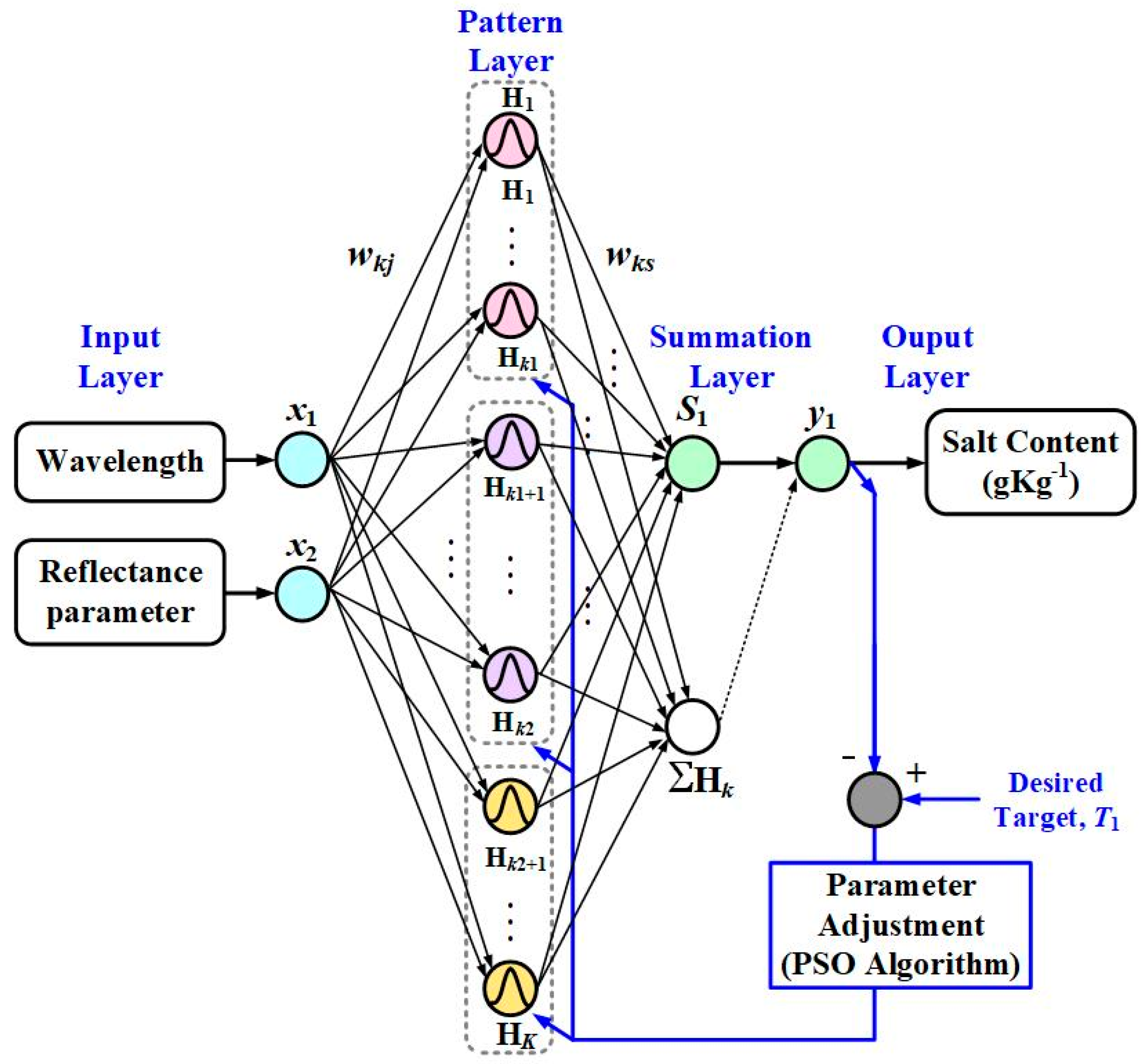
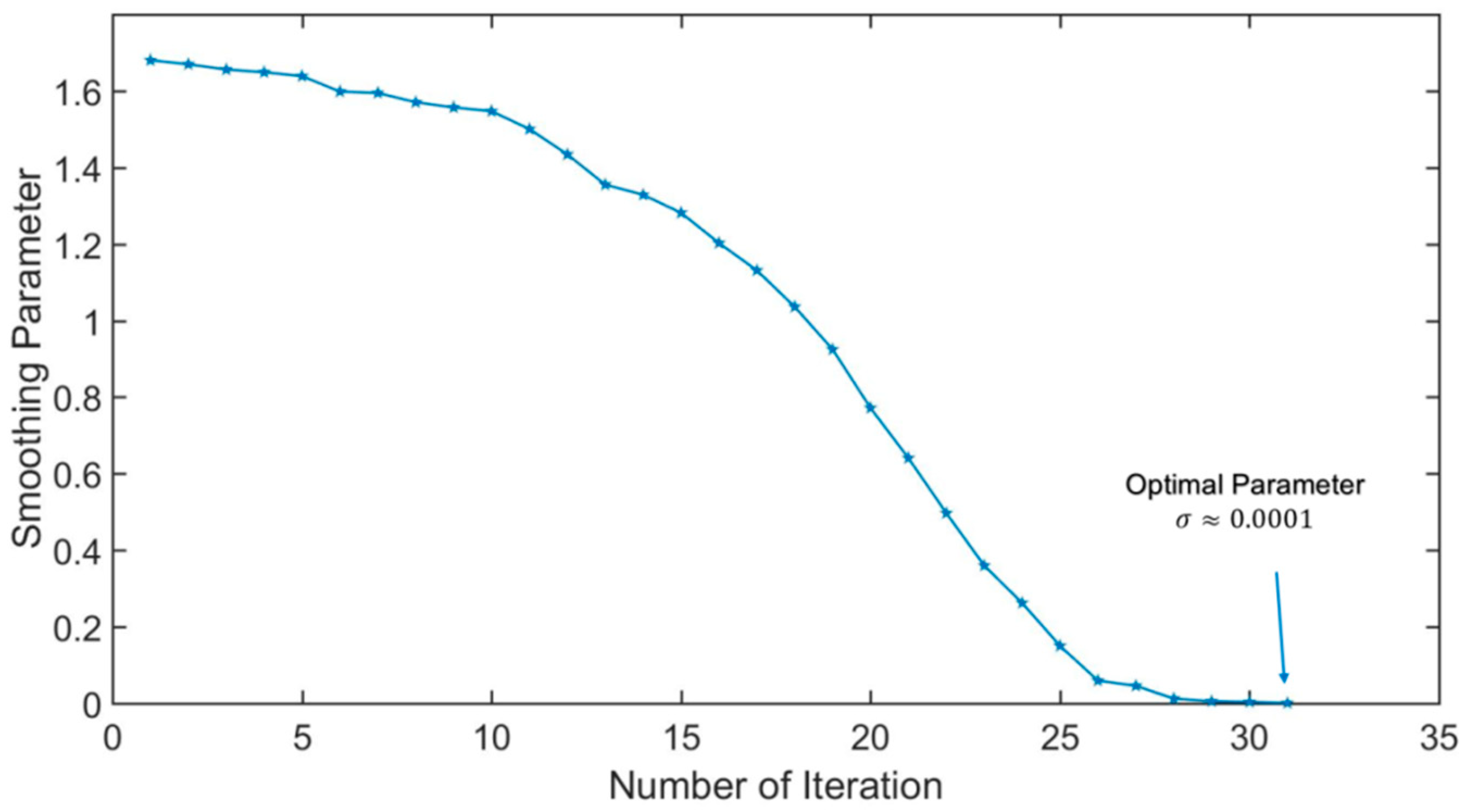
To overcome the poor prediction of linear PLSR models and to avoid the heavy calculation load of non-linear ANN models, a probability neural network (PNN) model was proposed in this paper. Particle swarm optimization was used to adjust the optimal smoothing parameter of the PNN model and to avoid the long training process required by a traditional neural network. In order to show the effects of human activities, the optimized wave band regions with and without human activities are also discussed in this study.

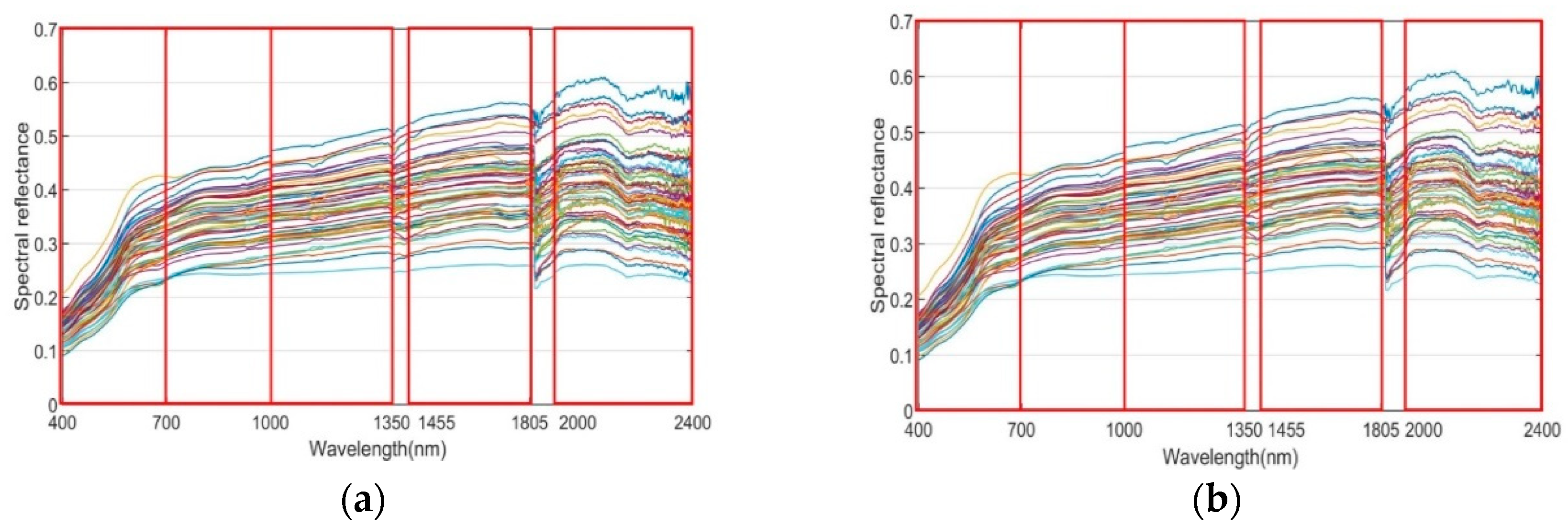
2. Data Collection

2.1. Overview of the Study Area

The test area is located in the Xinjiang Tianshan Northern Foothills at the southern edge of the Dzungarian Basin (87°44′–88°46′E, 43°29′–45°45′N). The soil categories include grey desert soil, cracked soil, and sandy soil. The research area was divided by a large channel, and two areas were selected (A and B), as shown in Figure 1. Because Area A is some distance from human habitation, it had not been developed and was considered to be free of human activities in this study. Area B is located near the Xinjiang 102 Production and Construction Army Corp and had been subject to human activity. Most of the land in Area B has been developed, some soils have been leveled, and some soils have been cultivated into tree seedlings; however, no fertilizer had been applied. The human activities in this area are very intensive. Thus, it was designated as having been subject to human activities.

2.2. Soil Sample Collection

In Area A, five sampling lines, spaced 600 to 800 m apart, were established in a north to south direction. In Area B, six sampling lines, spaced 800 to 1000 m apart, were set out. Five representative sampling points were selected along each sampling line. The interval between sampling points was 300 to 500 m. Area A had 25 sampling points, and Area B had 30 sampling points. Global positioning system (GPS) was used to determine the exact position of each of the 55 points. A soil sample was collected at a depth between 0 and 10 cm at each of the sampling points and placed in a sequentially numbered bag. The samples were air-dried in the laboratory, and their impurities were removed. After screening through a 1-mm sieve, the samples were sent to the Xinjiang Institute of Ecology and Geography to be tested for salt content.

2.3. Obtaining Spectrum Data

In this study, a portable FieldSpec^® 3 Hi-RES Spectrometer (ASD, USA) was used to collect soil spectrum data. The instrument has an effective spectral testing range between 350 and 2500 nm. The sampling interval is 1.4 nm at 350 to 1000 nm and 2 nm at 1000 to 2500 nm. The repeatability interval is 1 nm. Because weather conditions can affect the readings, spectral measurements were conducted from 9–23 May 2017, between 11:00 and 15:00 h, on clear cloudless days with no wind. Before each spectrum measurement, a whiteboard calibration was conducted to eliminate any dark current effects. The sensor head of the spectrometer was held 15 cm from the sampling point surface and directly above it when the reading was taken. To prevent surface cracks or surrounding vegetation from affecting the readings, each spectrum testing point chosen was situated away from any interfering objects. Spectrum readings were made at five different places, within a meter of each sampling point, and each reading was repeated 10 times. A total of 50 spectrum curves were obtained for each sampling point. The mean of these curves was used as the spectrum value for the sampling point.

3. Methodology

3.1. Probability Neural Network

PNN was proposed by Specht in 1991 for non-linear and high-dimensional mapping applications [35,36]. The PNN was designed to be similar to the multiple regression model and uses different wave bands and reflectance from various observation stations as the input variance, and the salt content reflects the relationship between output variances. PNN is formed from the input, pattern, summation, and output layers, as shown in Figure 2. In this study, particle swarm calculation was used to adjust the node parameters of the model, increase calculation speed of the PNN model, and avoid the huge volume of calculations required by the traditional ANN model.

PNN can provide large quantities of pattern nodes in the pattern layer and can approximate the non-linear prediction function or realize a non-linear prediction. Thus, the input vector X and output vector Y in the input layer and output layer can be expressed as an input-output match pattern, as shown in Equation (1):

$$\begin{gathered} X(k)=[x_1(k),x_2(k)]\to Y(k)=[y(k)] \\ {x}_1(k)=\lambda (k)/{\lambda }_{\max }, x_2(k)=R(k)/R_{\max } \\ y(k)=SC(k)/S{C}_{\max } \end{gathered}$$

(1)

where K is the quantity of data collected (k = 1, 2, ..., K), $\lambda (k)/{\lambda }_{\max }$ is the wavelength, $R(k)/R_{\max }$ is the reflectance, and $SC(k)/S{C}_{\max }$ is the salt content.

In this experiment, the pattern nodes can continue to grow while nodes are added or deleted in the pattern layer. This requires that the pattern nodes build a model in a short period of time for the high dimensional regression function and estimator. However, the input and output connect to the weight from the input nodes ($x_1$, $x_2$) to the pattern nodes ($H_1,H_2,\dots ,H_k,\dots ,H_K$) and the summation nodes ($S_1,{\displaystyle \sum H_K}$). The pattern node parameters require adjustment for the optimal calculation method. The PNN calculation steps are as follows:

Step 1. Consider that the K input-output matching training pattern can easily determine the multilayer network structure. There are two inputs, a K pattern, summation nodes, and one output node.

Step 2. For the 2 × K input training pattern $X(k)=[x_1(k),x_2(k)]$, the input layer and pattern layer relationship weight $w_{kj},j=1,2;k=1,2,3,\dots ,K$ is shown in Equation (2):

$$W^1={[w_{kj}]}^T={\left[\begin{array}{cc}{x}_1(k),& x_2(k)\end{array}\right]}^T$$

(2)

where ${[w_{kj}]}^T$ is the K × 2 matrix in this study, and $x_1(k),x_2(k)$ are K × 1 column vectors.

Step 3. For the K × 1 output training pattern (salt content), the pattern layer and summation layer relationship weight is $w_{ks},s=1,2$, as shown in Equation (3)

$$W^2={[w_{ks}]}^T={[\begin{array}{cc}y(k),& 1\end{array}]}^T$$

(3)

where $W^2={[w_{ks}]}^T$ is the K × 2 matrix, and $y(k)$ is K × 1 column vector. The total pattern to summation layer relationship weight ${\displaystyle \sum H_k}$ is set as 1.

Step 4. Calculate the output nodes $H_k,k=1,2,\dots ,K$ using the Gaussian function as in Equation (4):

$$H_k=\exp [-{\displaystyle \sum _{k=1}^K\frac{{(x_j(0)-w_{kj})}^2}{2{\sigma }_k^2}}]$$

(4)

where $X(0)={\left[\begin{array}{cc}{x}_1(0),& x_2(0)\end{array}\right]}^{}$ is the test pattern, and $\sigma ={\sigma }_1=\dots ={\sigma }_k=\dots ={\sigma }_K$ is the smoothing parameter. In this study, we used particle swarm optimization (PSO) [37] to search for the optimal parameter.

Step 5. Obtain $y_1$ of the output layer, as shown in Equation (5):

$$y_1={\displaystyle \sum _{k=1}^K{w}_{ks}\times H_k}/{\displaystyle \sum _{k=1}^{K}1\times H_k}=S_1/{\displaystyle \sum _{k=1}^K{H}_k}$$

(5)

The final output is shown in Equation (6):

$$SC=y_1\times S{C}_{\max }$$

(6)

After determining the output value, the RMSE can be used to show whether the prediction result of this model is accurate. The smaller the value, the more accurate the prediction, as shown in Equation (7):

$$\mathrm{RMSE}=\sqrt{\frac{1}{K}{\displaystyle \sum _{i=1}^K{\left(Y_i-Y_i{}^{\prime }\right)}^2}}$$

(7)

where $Y_i-Y_i{}^{\prime }$ is the error between the prediction value and the actual value.

3.2. Particle Swarm Optimization

In particle swarm optimization (PSO), the particle swarm [38] can reach up to 30 particles (experience: 10–30 particles). By separating particle swarms into numerous individual units we can separate the many possible optimal solutions. First, we move towards the target from all sides. In each optimal solution search process, the most advantageous particle from the particle swarm is selected, which is the optimal solution to mathematical problems. A global search method is used to move towards the target. PSO uses iteration to adjust the smoothing parameter $\sigma$:

Smoothing parameter correction calculation $\Delta \sigma$:

$$\Delta {\sigma }_g^{p+1}=\Delta {\sigma }_g^p+c_{1}ran{d}_1(\sigma bes{t}_g-{\sigma }_g^p)+c_{2}ran{d}_2(\sigma best-{\sigma }_g^p)$$

(8)

Adjustment parameter:

$$c_1=(b_1-a_1)\frac{p}{p_{\max }}+a_1,c_2=(b_2-a_2)\frac{p}{p_{\max }}+a_2$$

(9)

Smoothing parameter correction equation:

$${\sigma }_g^{p+1}={\sigma }_g^p+\Delta {\sigma }_g^{p+1}$$

(10)

where g = 1, 2, 3, …, G is the number of the particle swarm, σ best is the (p–1) optimal solution reached by iteration, and σ best_g is the optimal solution found by the g^th particle. Parameters rand₁ and rand₂ are the random values between 0 and 1; p is the iteration number and p_max is the maximum iteration number; c₁ and c₂ parameters can be used to adjust the number of iterations, a₁, a₂, b₁, and b₂, so that c₁ decreases from 2.5 to 0.5 (the individual coefficient) and c₂ increases from 0.5 to 2.5 (the group coefficient). Δσ_g^p+1 represents the distance of each particle swarm, that is, Δσ_g^p+1 is the time change adjustment parameter. During the search process, the initial phase allows the particles to move significantly towards the target. This method prevents the search from being confined to a small range. Once the target is near, the distance is reduced to search for the global optimal solution.

3.3. Model Verification

After the model was built, we used the prediction root mean square error (RMSE), coefficient of determination ($R^2$) and ratio of performance to deviation (RPD) to verify the predictive ability of the model [39,40]. The smaller the value of RMSE, the more precise the prediction of the model. The scope of the coefficient of determination lies in the range of $-1<R^2<1$. A value close to −1 represents a negative correlation, while a value close to 1 represents a positive correlation. The higher the model stability and fitting level, the closer $R^2$ will be to 1. When $\mathrm{RPD}\le 1.4$, the model will be unreliable, whereas the model prediction reliability is normal when $1.4<\mathrm{RPD}<2$. An $\mathrm{RPD}\ge 2$ indicates a model with a superior prediction ability. The RPD evaluation indicator is shown in Equation (11):

$$\mathrm{RPD}=\frac{\mathrm{SD}}{\mathrm{RMSE}}$$

(11)

where SD is the standard deviation.

4. Spectrum Data Pre-Processing

The component and structural information of the tested sample reside in the visible light, near-infrared and ultraviolet spectrum data. However, the instrument background, sample size, and other factors can affect the data and cause a baseline shift, random noise, light scattering, and other system activities. These activities can mask information and have a significant effect on the building of models and the determination of unknown sample components or properties. Such noisy spectra require pre-processing to reduce or eliminate the effects of various non-target factors before quantitative analysis can be done, and this is crucial for building a good stable model. Preprocessing can even have a decisive effect on the final result. Commonly used spectrum pre-processing methods include removing the interfering wave bands, the use of a smoothing algorithm, and mathematical transformation.

4.1. Removing Interfering Wave Bands

The spectra collected by the ASD device range from 350 nm to 2500 nm, with a total of 2150 bands, for uniform soils of the same kind. The smaller the spectrum curve fluctuation, the better the quality of the spectrum. The 350–399 nm ultraviolet and the 2401–2500 nm short-wave infrared bands have a poor reflectance signal to noise ratio, and the data from these segments are unreliable. Data from sampling point 15 in Area A, as examples of this low quality, are shown in Figure 3. The moisture absorption segments at 1400 nm, 1900 nm, and 2200 nm also show a significant curve fluctuation because of soil moisture. Moisture present in soil can have three forms, combination water, hygroscopic water, and pore water, which all fall within the same spectrum absorption wave band. Studies show that the absorption band near 1400 nm is the main hydroxyl-OH spectrum band, and the band near 1900 nm is the main inter-layer H₂O spectrum band [41,42,43,44,45]. The 2200 nm range includes hydroxyl stretching and Al-OH/Mg-OH bending vibrations, which have a greater effect on salt content spectrum inversion, as shown in Figure 4a. For these reasons, the reflectance from 350–399 nm, 2401–2500 nm, 1355–1410 nm, and 1820–1942 nm were removed, as shown in Figure 4b. The remaining 1823 wave bands from the soil sample reflectance spectrum data were used to build the inversion model.

4.2. Savitzky-Golay Convolution Smoothing

Savitzky-Golay (SG) convolution smoothing, also called polynomial smoothing, is widely used for spectrum filtering. The method combines least squares fitting with a moving window. First, a window that contains an odd number of points is selected. Each point of the spectrum in the window is perceived as a polynomial. Least squares is used to integrate the polynomial coefficient value. The calculation equation is as shown below:

$$X_{k,smooth}=\frac{1}{H}{\displaystyle \sum _{i=-w}^{+w}{x}_{k+i}{h}_i}$$

(12)

where $h_i$ is the smoothing coefficient and can be obtained through polynomial fitting. H is the normalization factor, for which the calculation method is $H={\displaystyle \sum _{i=-w}^{+w}{h}_i}$.

4.3. Multiple-Spectrum Mathematical Transformation

Before a model based on spectral reflectance of earth surface parameters is calculated and built, the original spectral reflectance (R) is often used to implement non-linear mathematical transform-ation. Commonly used non-linear mathematical transformations include root mean square ($\sqrt{R}$), reciprocal (1/R), inverse logarithmic (log(1/R)), logarithmic (log(R)), and logarithmic reciprocal (1/log(R)). There are two reasons for this. (1) To make the linear relationship between spectral reflectance and earth surface non-linear, so that simple linear regression analysis can be conducted to obtain an approximate non-linear result. By building different forms of an estimation model, an optimal model can be selected to increase the precision of identification. (2) To use non-linear transformation to increase spectrum difference so that the earth surface parameters will have a discernible effect on the spectrum. The original spectral reflectance R from sampling point 15 in Area A, along with five types of spectral transform form curve, is shown in Figure 5.

5. Simulation Results

5.1. Five Wave Band Intervals

As described in Section 4.1, 1823 wave bands were used to build the soil salt content inversion model after the noise and moisture absorption wave bands had been removed. Of these 1823 bands, some had a rather weak correlation with salt content. The inclusion of these bands would have interfered with the building of the model as well as its prediction and precision. To find the optimal wave band interval for building the inversion model, we avoided those affected by moisture and extracted five wave band intervals, as shown in Figure 6. The bands include one visible light band (400–700 nm) and four near-infrared bands (700–1000 nm, 1000–1350 nm, 1455–1805 nm, and 2000–2400 nm). The lengths of the five wave band intervals were 300 nm, 300 nm, 350 nm, 350 nm, and 400 nm. Referencing Zhao [46], we changed the reflectance R to $\sqrt{R}$, $1/R$, $\log (1/R)$, $\log (R)$, and $1/\log (R)$, and introduced them separately into the probability neural network model to determine the best band interval.

5.2. Optimal Smoothing Parameter

The only parameter that required adjustment in PNN was the smoothing parameter. The accuracy of the PNN network output is affected by the smoothing parameters, and adjustment can produce K number of classifiers in the pattern layer. In this study, we used a Gaussian function to conduct a similarity comparison between the input pattern and training pattern. The classifier of each Gaussian function attempts to give its target value maximum similarity. Therefore, an appropriate σ parameter should be chosen. Assume that the target function/squared error function is:

$$T(k)=E(y(x_k)|x_k),SEF={\displaystyle \sum _{k=1}^K{[T(k)-y(k)]}^2}\le {\epsilon }_k$$

(13)

where T(k) is the preset target vector, and its physical purpose is the expression and adjustment of parameter $\sigma$. ${\epsilon }_k$ is the tolerable error value that allows the actual output value of the PNN to be near the target value. This conforms to the trend of the target function/squared error function value becoming smaller.

Before the simulation experiment, the neural network model must find the optimal smoothing parameter $\sigma \approx 0.0001$ (see Figure 7) so that the model can enable a simulation comparison.

5.3. Evaluation Indicators for Area A

As previously mentioned, the study area was divided into Areas A and B. The spectral reflectance at the five wave band intervals were used as the inputs. The output was the salt content. The precision evaluation index values of RMSE, $R^2$, and RPD for the three models were calculated. Area A is used as the first discussion subject. The summary is shown in

Table 1. The root mean square error (RMSE) value of the probability neural network (PNN) model in Area A.

Wavelength	Signal	R	$\sqrt{\mathit{R}}$	1/R	log(1/R)	log(R)	1/log(R)
400–700 nm	Original	0.880219	0.846142	0.24551	0.432957	0.432957	0.623002
	SG	0.88395	0.851433	0.227578	0.4545	0.4545	0.634666
700–1000 nm	Original	0.666516	0.715382	0.237389	0.413956	0.413956	0.4538
	SG	0.669802	0.718228	0.293012	0.445924	0.445924	0.479089
1000–1350 nm	Original	0.503986	0.574182	0.18463	0.313566	0.313566	0.303839
	SG	0.512374	0.5803	0.140863	0.303304	0.303304	0.290997
1455–1805 nm	Original	0.98773	1.092727	0.319539	0.598944	0.598944	0.587325
	SG	0.997925	1.103375	0.350219	0.61947	0.61947	0.610725
2000–2400 nm	Original	0.600098	0.663767	0.211646	0.368735	0.368735	0.360034
	SG	0.659119	0.711643	0.322248	0.466626	0.466626	0.460637

,

Table 2. The $R^2$ value of the PNN model in Area A.

Wavelength	Signal	R	$\sqrt{\mathit{R}}$	1/R	log(1/R)	log(R)	1/log(R)
400–700 nm	Original	0.980265	0.981634	0.998564	0.995391	0.995391	0.990327
	SG	0.980088	0.981386	0.998599	0.994626	0.994626	0.989803
700–1000 nm	Original	0.993754	0.992662	0.994437	0.997762	0.997762	0.997385
	SG	0.993514	0.992418	0.998454	0.997112	0.997112	0.996863
1000–1350 nm	Original	0.994176	0.992279	0.999183	0.997733	0.997733	0.99795
	SG	0.993888	0.992063	0.999374	0.997755	0.997755	0.99801
1455–1805 nm	Original	0.97765	0.972195	0.998362	0.992584	0.992584	0.992823
	SG	0.97698	0.971436	0.997082	0.991397	0.991397	0.991483
2000–2400 nm	Original	0.991189	0.989169	0.999038	0.996719	0.996719	0.996814
	SG	0.988771	0.987007	0.997086	0.993908	0.993908	0.993993

and

Table 3. The ratio of performance to deviation (RPD) value of the PNN model in Area A.

Wavelength	Signal	R	$\sqrt{\mathit{R}}$	1/R	log(1/R)	log(R)	1/log(R)
400–700 nm	Original	6.400056	6.657809	22.94595	13.01157	13.01157	9.042428
	SG	6.373043	6.616435	24.75394	12.39483	12.39483	8.876255
700–1000 nm	Original	8.452091	7.874745	23.7309	13.60883	13.60883	12.41394
	SG	8.410621	7.843541	19.22602	12.63322	12.63322	11.75867
1000–1350 nm	Original	11.17781	9.811266	30.51219	17.96574	17.96574	18.54091
	SG	10.9948	9.707836	39.99251	18.57365	18.57365	19.35916
1455–1805 nm	Original	5.703437	5.155406	17.62992	9.405647	9.405647	9.591717
	SG	5.645165	5.105654	16.0855	9.09399	9.09399	9.224208
2000–2400 nm	Original	9.38756	8.487099	26.61728	15.27779	15.27779	15.64701
	SG	8.546946	7.916121	17.48176	12.07275	12.07275	12.2297

.

The smallest RMSE value within the 1000–1350 nm range was 0.140863, as shown in Table 1, and this was introduced into the PNN model using SG spectrum smoothing and the $1/R$ method.

The largest $R^2$ value within the range of 1000–1350 nm was 0.999374, as shown in Table 2, and this was introduced into the PNN model using SG spectrum smoothing and the 1/R method.

The largest RPD value within the range of 1000–1350 nm was 39.99251, as shown in Table 3, and this was introduced into the PNN model using SG spectrum smoothing and the $1/R$ method.

In Area A with no human activities, the three evaluation indicators of the PNN model (RMSE, $R^2$, and RPD) were all located on the same band interval of 1000–1350 nm, as shown in Table 1, Table 2 and Table 3. The same signal source SG smoothing spectrum, as well as the same mathematical transformation and $1/R$ method, were used. The three index values showed outstanding results, the coefficient of determination $R^2$ was 0.999374, and the corresponding prediction ability RPD was 39.99251. The $R^2$ value was very near 1, and the RPD value was far greater than 2. This showed that the PNN model had an excellent prediction ability, and the prediction results were very good.

5.4. Area A Prediction Results

The prediction results and linear fitting for Area A are shown in Figure 8. The prediction result of the PNN model in the 1000–1350 nm band, where SG spectrum smoothing and $1/R$ were used to introduce the segment into the neural network model, is shown in Figure 8a. Blue represents the salt content prediction value and red represents the actual measured salt content value. Yellow is the error between the prediction value and actual measured value. The linear fitting result for the PNN model is shown in Figure 8b.

The PNN model had slight prediction errors at observation points 2, 11, 13, 14, and 15, as shown in Figure 8a. The mean error was 0.0084012 (g/kg). Overall, however, the prediction ability was very good. For linear fitting, the coefficient of determination $R^2$ of the PNN model reached 0.99937, which is very close to 1, as shown in Figure 8b. This shows that the stability and fit of the PNN model was very high.

5.5. Area B Evaluation Indicators

The spectral reflectance and five wave band intervals were used (as in Area A) as the input while the salt content was the output in calculating the precision evaluation index values of RMSE, $R^2$, and RPD for the PNN model (

Table 4. The RMSE value of the PNN model in Area B.

Wavelength	Signal	R	$\sqrt{\mathit{R}}$	1/R	log(1/R)	log(R)	1/log(R)
400–700 nm	Original	1.652057	1.578996	0.362379	0.755131	0.755131	1.10885
	SG	1.395946	1.33715	0.281027	0.658492	0.658492	0.984695
700–1000 nm	Original	1.881389	2.027826	0.670349	1.195093	1.195093	1.270434
	SG	1.885963	2.034313	0.741881	1.177413	1.177413	1.253372
1000–1350 nm	Original	1.172402	1.277664	0.416209	0.684781	0.684781	0.676523
	SG	1.171473	1.277971	0.506309	0.725767	0.725767	0.720614
1455–1805 nm	Original	0.940534	1.066988	0.331386	0.573277	0.573277	0.518566
	SG	0.962209	1.087288	0.338851	0.623245	0.623245	0.579542
2000–2400 nm	Original	1.264737	1.395243	0.574168	0.894886	0.894886	0.823833
	SG	1.083877	1.263583	0.358336	0.582145	0.582145	0.508204

,

Table 5. The $R^2$ value of the PNN model in Area B.

Wavelength	Signal	R	$\sqrt{\mathit{R}}$	1/R	log(1/R)	log(R)	1/log(R)
400–700 nm	Original	0.981787	0.98322	0.999088	0.996064	0.996064	0.992045
	SG	0.989466	0.99	0.999208	0.998047	0.998047	0.995474
700–1000 nm	Original	0.967022	0.961644	0.995763	0.986701	0.986701	0.984855
	SG	0.966294	0.960977	0.994643	0.986877	0.986877	0.985058
1000–1350 nm	Original	0.990661	0.989318	0.998602	0.996765	0.996765	0.996747
	SG	0.990562	0.989185	0.998028	0.996127	0.996127	0.996085
1455–1805 nm	Original	0.995222	0.993748	0.999069	0.998343	0.998343	0.998549
	SG	0.994733	0.993217	0.999017	0.997754	0.997754	0.997931
2000–2400 nm	Original	0.984271	0.981215	0.996815	0.992047	0.992047	0.99292
	SG	0.990315	0.986701	0.996413	0.99785	0.99785	0.998264

and

Table 6. The RPD value of the PNN model in Area B.

Wavelength	Signal	R	$\sqrt{\mathit{R}}$	1/R	log(1/R)	log(R)	1/log(R)
400–700 nm	Original	6.047578	6.327404	27.5704	13.23074	13.23074	9.010187
	SG	7.157114	7.47182	35.55161	15.17245	15.17245	10.14623
700–1000 nm	Original	5.310409	4.926924	14.9041	8.359976	8.359976	7.864198
	SG	5.29753	4.911213	13.46704	8.485507	8.485507	7.971253
1000–1350 nm	Original	8.521775	7.819697	24.00465	14.58998	14.58998	14.76808
	SG	8.528532	7.817816	19.73291	13.76605	13.76605	19.26648
1455–1805 nm	Original	10.62263	9.363695	30.149	17.42778	17.42778	19.26648
	SG	10.38334	9.188868	29.48481	16.03053	16.03053	17.23937
2000–2400 nm	Original	7.899625	7.160722	17.40074	11.16449	11.16449	12.12738
	SG	9.217781	7.906835	27.88154	17.1623	17.1623	19.65932

).

The smallest RMSE value within the range of 400–700 nm was 0.281027, as shown in Table 4, and this was introduced into the PNN model using SG spectrum smoothing and the $1/R$ method.

The largest $R^2$ value within the range of 400–700 nm was 0.999208, as shown in Table 5, and this was introduced into the PNN model using SG spectrum smoothing and the $1/R$ method.

The largest RPD value within the range of 400–7000 nm was 35.55161, as shown in Table 6, and this was introduced into the PNN model using SG spectrum smoothing and the $1/R$ method.

From Table 4, Table 5 and Table 6, it can be seen that the three PNN model evaluation indicators (RMSE, $R^2$, RPD) were all located on the same band interval, 400–700 nm in Area B. The same signal source SG spectrum smoothing and $1/R$ mathematical transformation were used, and the three index values provided very good results. The coefficient of determination $R^2$ was 0.999208, and the corresponding prediction ability RPD was 35.55161. The $R^2$ value was very close to 1, and the RPD value was much greater than 2. This indicated that the prediction ability of the PNN model was very good. Although the RPD value of Area B (35.55161) was lower than that of Area A (39.99251), both were far greater than 30. This indicated that the PNN model was suitable for use in undisturbed as well as disturbed areas, and it was capable of giving outstanding results. Area B had been subject to human activities, and the soil had been disturbed, but the soil in Area A had remained in its natural undisturbed state. Thus, the PNN prediction ability was lower for Area A.

5.6. Area B Prediction Results

Area B prediction results and linear fit are shown in Figure 9. The prediction result for the 400–700 nm range in the PNN model, which was introduced into the neural network using SG spectrum smoothing and the $1/R$ method, is shown in Figure 9a. The salt content prediction values are blue, and the actual measured salt content values are red. Yellow indicates the error between the prediction values and actual measured values. The linear fitting result for the PNN is shown in Figure 9b.

More than half of the observation points exhibited a slight error in the PNN model, and the mean error value was 0.015297 (g/kg), as shown in Figure 9a. The errors were small, and the overall prediction ability of the model was very good. The coefficient of determination $R^2$ of the PNN model reached 0.99921, as shown in the linear fitting in Figure 9b. This is also very close to 1, indicating very high stability and fit in Area B.

6. Discussion

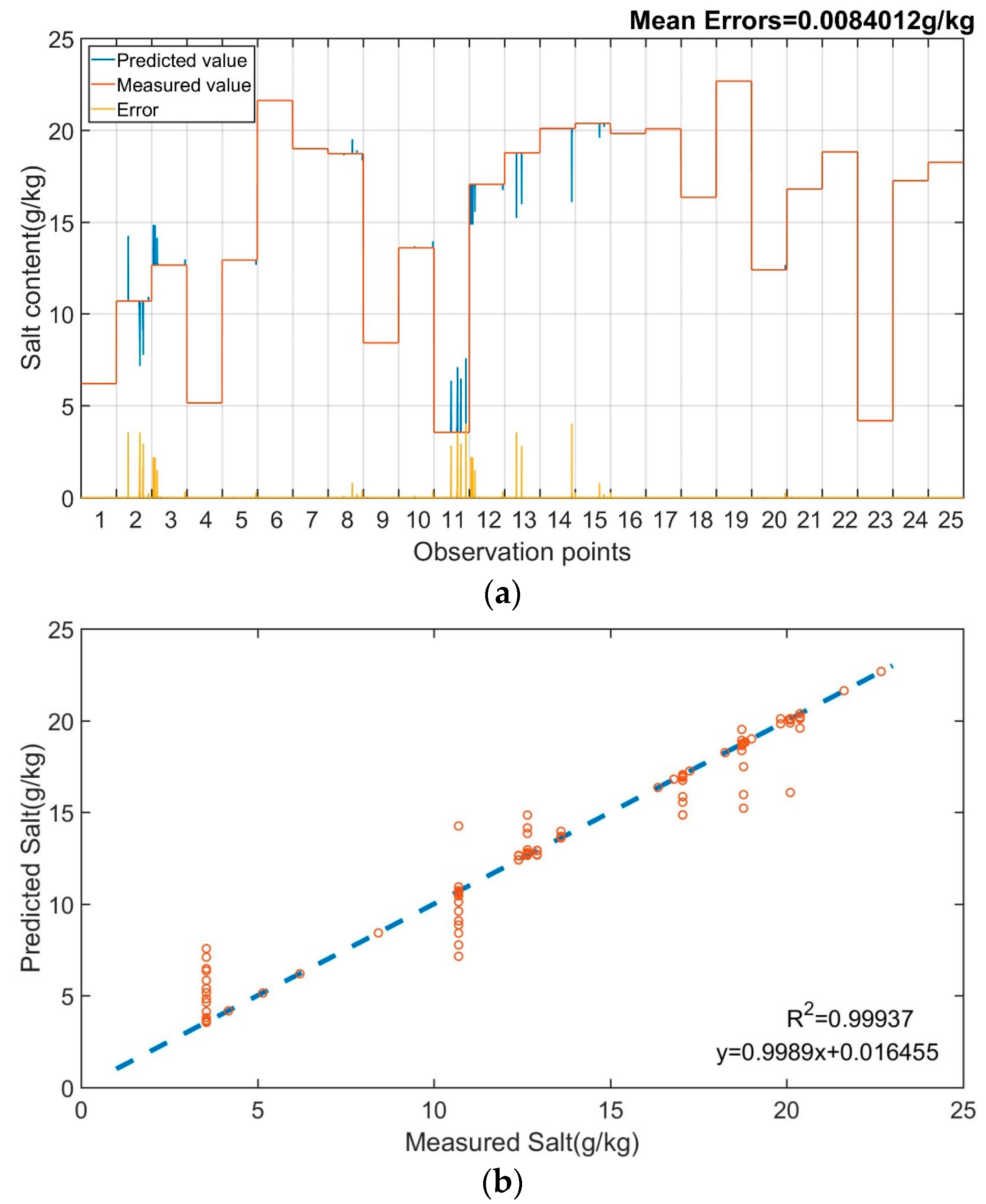
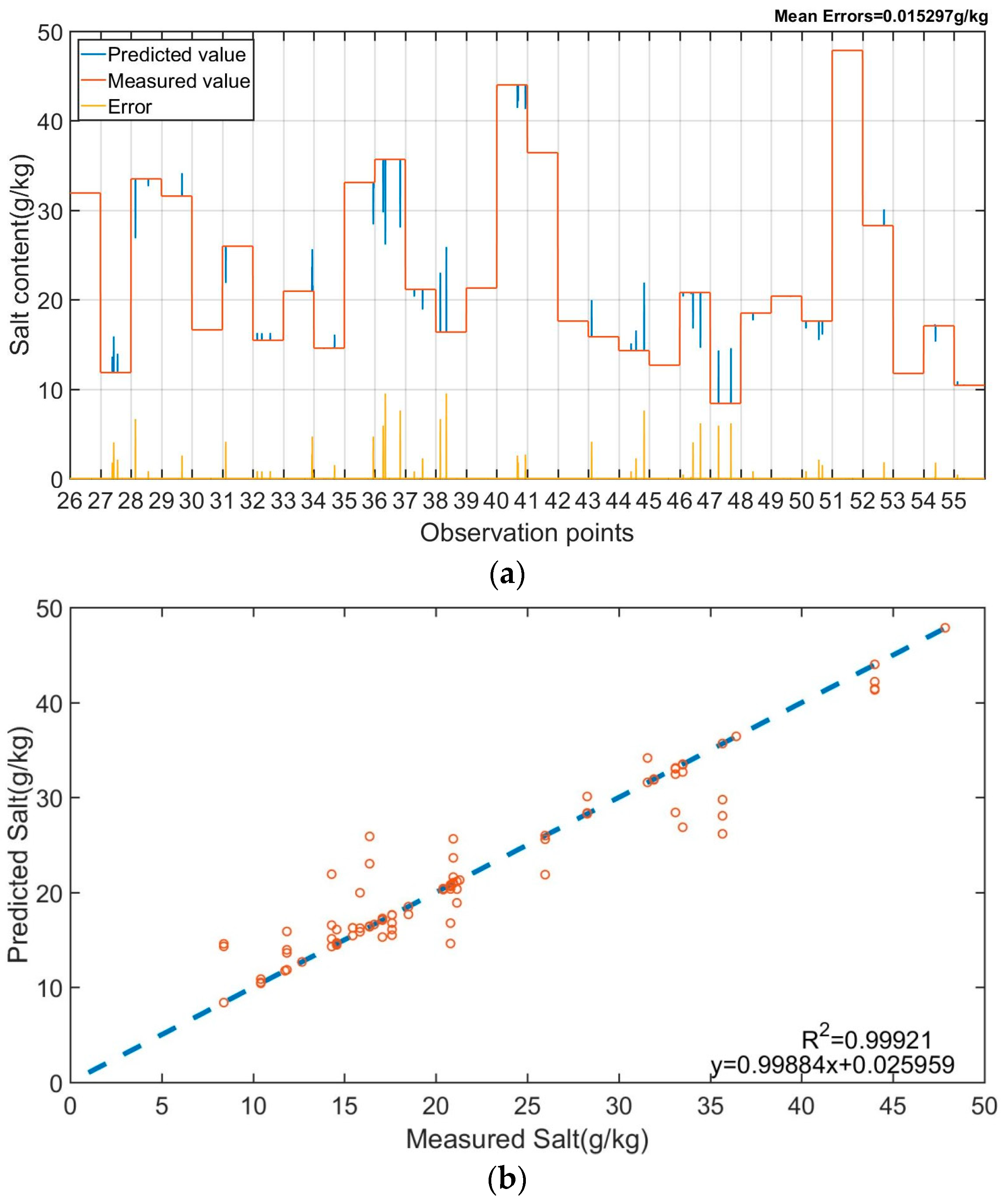
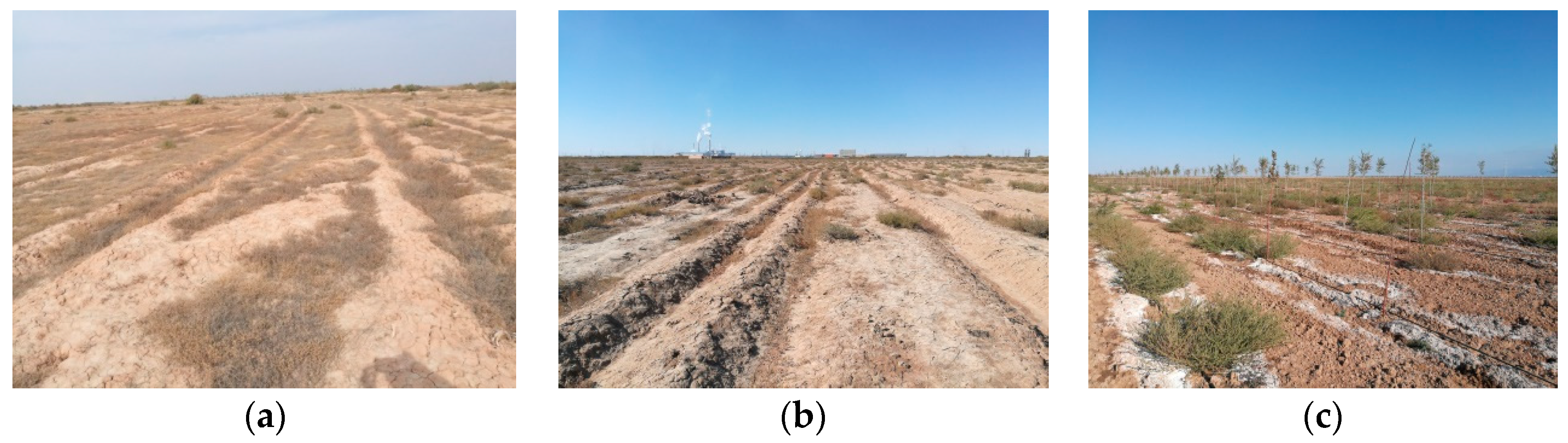
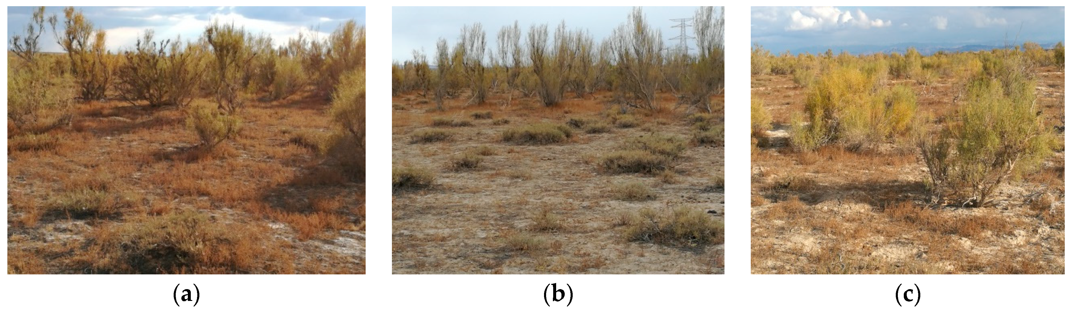
The PNN model had a better performance in Area A than in Area B with respect to prediction. The main reason for this was that Area B had been disturbed by plowing, as shown in Figure 10. The soil surface had undergone different degrees of damage, and the soil moisture and salt content shifts were more complex. These factors interfered with the features of the soil spectrum. Area A had remained more or less in its natural state, as shown in Figure 11, and the prediction ability of the PNN model was better. The results also showed that the optimal band interval in the PNN model was 1000–1350 nm, under near-infrared short-wave bands, and 400–700 nm, under visible light bands, for Area A and Area B, respectively. The results obtained in this study were consistent with the similar band intervals of previous studies [47,48,49,50]. Previous researchers used spectroscopy to predict salt content and found that the optimal band was also in the visible light and near-infrared short-wave bands.

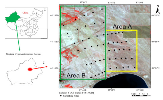
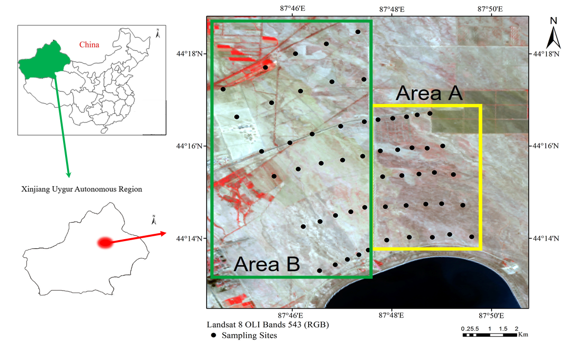
We conducted a field investigation of the study areas in 2016. The study areas are located near the Xinjiang 102 Construction Army Corp. It was found that there is a huge canal between Area A and Area B, which is 24 m wide at the highest point, 6 m wide at the lowest point, 5 m deep, and 15.3 km long. We divided the two different regions using the canal as a boundary.

From an analysis of different soil properties caused by human activities, it can be seen that Area A is far from human settlement, and is rarely affected by human activities due to the area’s isolation caused by the huge canal. This area basically has maintained its original ecological environment. However, Area B is very close to the location of 102 Construction Army Corp, and some houses in human settlements can be seen in Figure 10b, indicating that the human activities in this area are very intensive. Therefore, the soil properties caused by human activities in the two areas are significantly different.

From an analysis of the soil cover environment, it can be seen that there are some haloxylon, red willow, and salt claw in the soil surface of Area A. Due to the small range of soil spectral tests, we chose to perform spectral measurements at locations where the soil surface is covered by less vegetation. However, most of the land in Area B has been developed, and some soils have been leveled, as shown in Figure 10a,b. At the same time, some soils in Area B have been cultivated into tree seedlings, as shown in Figure 10c. Particularly in Figure 10c, we can see that there are some white salts on the surface of the soil, indicating that the salinization of this area is very extensive. Therefore, the soil cover environment in the two areas is differs significantly.

Moreover, in the process of land use and development in arid and semi-arid regions, the oasis ecological environment is under different degrees of human activity. The differences in the stress of human activities on the oasis ecological environment are mainly manifested in two aspects. The first is the difference in land use patterns and intensity. Second, there is a big difference in the duration of land use. Therefore, during the development and utilization of land, regular and irregular irrigation and the construction of ditches and networks will lead to a spatial imbalance of regional water. At the same time, the consolidation and development of land will directly change the local soil structure and type, causing changes in salt transport channels and transfer rates, which in turn exacerbate the complexity of salt spatial variability.

Finally, human activities refer to people controlling the development direction of the soil by changing a certain soil-forming factor or changing the contrast between various factors. For example, eliminating the original natural vegetation and replacing it with artificially cultivated crops or artificial vegetation can directly and indirectly affect the direction and intensity of the biological cycle of the soil. Irrigation and drainage can change the hydrothermal conditions of natural soils, thus changing the migration and transformation process of substances in the soil. Agricultural practices, such as farming and fertilization, can directly affect soil development, soil material composition and shape changes.

7. Conclusions

The results of this study show that after signal pre-processing was complete and the band had been selected, the mathematical introduction of PSO optimization into the PNN model using the $1/R$ method produced optimal results. The predictive ability indicator RPD for the PNN model with PSO optimization was greater than 30 in both Areas A and B, providing a clear indication of an excellent predictive ability. The results indicated that the optimal wave band intervals for PNN modeling differed in areas affected and non-affected by human activities. The optimal interval of the artificial activities region falls in the visible light band, and the optimized wave band region without human activities falls outside the visible light band. It was shown that the near-infrared short-wave bands in the range of 1000–1350 nm can be used to analyze undisturbed areas, and the visible light bands in the range of 400–700 nm are more suitable for analyzing areas that have been disturbed by human activities in Xinjiang, China. The $R^2$ of the PNN model for Area A was 0.999374, and the RPD was 39.99251. The $R^2$ of the PNN model for Area B was 0.999208, and RPD was 35.55161. The results of this study could provide a reference point for aircraft or satellite-carried remote sensing technology, large-scale soil salinization monitoring, salinization data extraction, and remote sensing topic mapping. The results can also be used as a reference point for the monitoring of other soil surface parameters, such as organic matter, pH value, and nitrogen, phosphorus, potassium, cation, and anion content. Lastly, the results of this study provide a new perspective in the hyperspectral technology monitoring of soil salinization in areas with different levels of human activities.

References

1. Nawar, S.; Buddenbaum, H.; Hill, J. Digital mapping of soil properties using multivariate statistical analysis and ASTER data in an arid region. Remote Sens. 2015, 7, 1181–1205. [Google Scholar] [CrossRef]
2. Ding, J.L.; Yu, D.L. Monitoring and evaluating spatial variability of soil salinity in dry and wet seasons in the Werigan-Kuqa Oasis, China, using remote sensing and electromagnetic induction instruments. Geoderma 2014, 235, 316–322. [Google Scholar] [CrossRef]
3. Marcos, R.G.; Fauze, A.A.; André, R.F.; Alessandro, F.M.; Alexandre, T.P.; Magali, F.T.D.; Adley, F.R.; Edvani, C.M. Superabsorbent hydrogels based on polysaccharides for application in agriculture as soil conditioner and nutrient carrier: A review. Eur. Polym. J. 2015, 72, 365–385. [Google Scholar]
4. Hu, G.T.; He, D.; Kenneth, A.S. Soil phosphorus and potassium estimation using visible-near infrared reflectance spectroscopy with direct orthogonal signal correction. Trans. Chin. Soc. Agric. Mach. 2015, 46, 139–145. [Google Scholar]
5. Li, J.G.; Pu, L.J.; Han, M.F.; Zhu, M.; Zhang, R.S.; Xiang, Y.Z. Soil salinization research in China: Advances and prospects. J. Geogr. Sci. 2014, 24, 943–960. [Google Scholar] [CrossRef]
6. McLeod, M.K.; Slavich, P.G.; Irhas, Y.; Moore, N.; Rachman, A.; Ali, N.; Iskandar, T.; Hunt, C.; Caniago, C. Soil salinity in Aceh after the December 2004 Indian Ocean tsunami. Agric. Water Manag. 2010, 97, 605–613. [Google Scholar] [CrossRef]
7. Metternicht, G.I.; Zinck, J.A. Remote sensing of soil salinity: Potentials and constraints. Remote Sens. Environ. 2003, 85, 1–20. [Google Scholar] [CrossRef]
8. Allbed, A.; Kumar, L.; Sinha, P. Mapping and modeling spatial variation in soil salinity in the Al Hassa Oasis based on remote sensing indicators and regression techniques. Remote Sens. 2014, 6, 1137–1157. [Google Scholar] [CrossRef]
9. Farifteh, J.; Farshad, A.; George, R.J. Assessing salt-affected soils using remote sensing, solute modeling, and geophysics. Geoderma 2006, 130, 191–206. [Google Scholar] [CrossRef]
10. Liu, S.L.; Maimaitiaili, B.; Joergensen, R.G.; Feng, G. Response of soil microorganisms after converting a saline desert to arable land in central Asia. Appl. Soil Ecol. 2016, 98, 1–7. [Google Scholar] [CrossRef]
11. Dinh, H.Q.; Fotedar, R. Early development of the blue mussel Mytilus edulis (Linnaeus, 1758) cultured in potassium-fortified inland saline water. Aquaculture 2016, 452, 373–379. [Google Scholar] [CrossRef]
12. Fan, X.; Pedroli, B.; Liu, G.; Liu, Q.; Liu, H.; Shu, L. Soil salinity development in the yellow river delta in relation to groundwater dynamics. Land Degrad. Dev. 2011, 23, 175–189. [Google Scholar] [CrossRef]
13. Weng, Y.; Gong, P.; Zhu, Z. Soil salt content estimation in the Yellow River delta with satellite hyperspectral data. Can. J. Remote Sens. 2008, 34, 259–270. [Google Scholar]
14. Herrero, J.; Netthisinghe, A.; Hudnall, W.H.; Pérez, C.O. Electromagnetic induction as a basis for soil salinity monitoring within a Mediterranean irrigation district. J. Hydrol. 2011, 405, 427–438. [Google Scholar] [CrossRef] [Green Version]
15. Ding, J.L.; Wu, M.C.; Tashpolat, T. Study on soil salinization information in Arid Region using remote sensing technique. Agric. Sci. Chin. 2011, 10, 404–411. [Google Scholar] [CrossRef]
16. Brunner, P.; Li, H.T.; Kinzelbach, W. Generating soil electrical conductivity maps at regional level by integrating measurements on the ground and remote sensing data. Int. J. Remote Sens. 2007, 28, 3341–3361. [Google Scholar] [CrossRef]
17. Sahu, N.; Singh, S.K.; Reddy, G.P.O.; Kumar, N.; Nagaraju, M.S.S.; Srivastava, R. Large-Scale Soil Resource Mapping Using IRS-P6 LISS-IV and Cartosat-1 DEM in Basaltic Terrain of Central India. J. Indian Soc. Remote Sens. 2016, 44, 811–819. [Google Scholar] [CrossRef]
18. Joshi, N.; Baumann, M.; Ehammer, A.; Fensholt, R.; Grogan, K.; Hostert, P.; Jepsen, M.; Kuemmerle, T.; Meyfroidt, P.; Mitchard, E.; et al. A review of the application of optical and radar remote sensing data fusion to land use mapping and monitoring. Remote Sens. 2016, 8, 1–23. [Google Scholar] [CrossRef]
19. Wu, W.C.; Mhaimeed, A.S.; Al-Shafie, W.M.; Ziadat, F.; Dhehibi, B.; Nangia, V.; Pauw, E.D. Mapping soil salinity changes using remote sensing in Central Iraq. Geoderma Regional. 2014, 23, 21–31. [Google Scholar] [CrossRef]
20. Lobell, D.B.; Ortizmonasterio, J.I.; Gurrola, F.C.; Valenzuela, L. Identification of saline soils with multiyear remote sensing of crop yields. Soil Sci. Soc. Am. 2007, 71, 777–783. [Google Scholar] [CrossRef]
21. Cao, L.; Ding, J.L.; Yu, H.Y. Relationship between multi-scale landscape pattern and salinity in Weigan and Kuqa rivers delta oasis. Trans. Chin. Soc. Agric. Eng. 2016, 32, 101–110. [Google Scholar]
22. Luan, F.M.; Zhang, X.L.; Xiong, H.; Zhang, F.; Wang, F. Comparative Analysis of Soil Organic Matter Content Based on Different Hyperspectral Inversion Models. Spectrosc. Spectr. Anal. 2013, 33, 196–200. [Google Scholar]
23. Han, Y.; Xu, W.R.; Jin, L. Study on the polarized reflectance hyperspectral characteristics and models of typical saline soil. J. Infrared Millim. Waves 2015, 34, 606–612. [Google Scholar]
24. Ding, J.L.; Wu, M.C.; Liu, H.X.; Li, Z.G. Study on the soil salinization monitoring based on synthetical hyperspectral index. Spectrosc. Spectr. Anal. 2012, 32, 1918–1922. [Google Scholar]
25. Viscarra, R.R.A.; Walvoort, D.J.J.; McBratney, A.B.; Janik, L.J.; Skjemstad, J.O. Visible, near infrared, mid infrared or combined diffuse reflectance spectroscopy for simultaneous assessment of various soil properties. Geoderma 2006, 131, 59–75. [Google Scholar] [CrossRef]
26. Debaene, G.; Niedźwiecki, J.; Pecio, A.; Żurek, A. Effect of the number of calibration samples on the prediction of several soil properties at the farm-scale. Geoderma 2014, 214, 114–125. [Google Scholar] [CrossRef]
27. Ben-Dor, E.; Patkin, K.; Banin, A.; Karnieli, A. Mapping of several soil properties using DAIS-7915 hyperspectral scanner data. A case study over clayey soils in Israel. Int. J. Remote Sens. 2002, 23, 1043–1062. [Google Scholar] [CrossRef]
28. Qu, Y.H.; Duan, X.L.; Gao, H.Y.; Chen, A.P.; An, Y.Q.; Song, J.L.; Zhou, H.M.; He, T. Quantitative retrieval of soil salinity using hyperspectral data in the region of Inner Mongolia Hetao irrigation district. Spectrosc. Spectr. Anal. 2009, 29, 1362–1366. [Google Scholar]
29. Liu, X.Y.; Shi, Z.Y.; Chang, Q.R.; Liu, C.Z.; Huang, M.; Gu, X. Hyperspectral Model for Estimation of Soil Potassium Content in Loessal soil. Acta Pedologica Sin. 2018, 55, 325–337. [Google Scholar]
30. Liu, X.M.; Liu, J.S. Based on the LS-SVM modeling method determination of soil available N and available K by using near-infrared spectroscopy. Spectros. Spectr. Anal. 2012, 32, 3019–3023. [Google Scholar]
31. Farifteh, J.; Meer, F.V.D.; Atzberger, C.; Carranza, E.J.M. Quantitative analysis of salt-affected soil reflectance spectra: A comparison of two adaptive methods (PLSR and ANN). Remote Sens. Environ. 2017, 110, 59–78. [Google Scholar] [CrossRef]
32. Weng, Y.L.; Gong, P.; Zhu, Z.L. A Spectral Index for Estimating Soil Salinity in the Yellow River Delta Region of China Using EO-1 Hyperion Data. Pedosphere 2010, 20, 378–388. [Google Scholar] [CrossRef]
33. Sidike, A.; Zhao, S.H.; Wen, Y.M. Estimating soil salinity in Pingluo County of China using QuickBird data and soil reflectance spectra. Int. J. App. Earth Obs. Geoinf. 2014, 26, 156–175. [Google Scholar] [CrossRef]
34. Zhang, X.G.; Huang, B.; Ji, J.F.; Hu, W.Y.; Sun, W.X.; Zhao, Y.C. Quantitative prediction of soil salinity content with visible-near infrared hyper-spectra in Northeast China. Spectrosc. Spectr. Anal. 2012, 32, 2075–2079. [Google Scholar]
35. Specht, D.F. Probabilistic neural networks. Neural Netw. 1990, 3, 109–118. [Google Scholar] [CrossRef]
36. Specht, D.F. A general regression neural network. IEEE Trans. Neural Netw. 1991, 2, 568–576. [Google Scholar] [CrossRef] [PubMed]
37. Yau, H.T.; Hung, T.H.; Hsieh, C.C. Bluetooth based chaos synchronization using particle swarm optimization and its applications to image encryption. Sensors 2012, 12, 7468–7484. [Google Scholar] [CrossRef] [PubMed]
38. Selvakumar, A.I.; Thanushkodi, K. A new particle swarm optimization solution to nonconvex economic dispatch problems. IEEE Trans. Power Syst. 2007, 22, 42–51. [Google Scholar] [CrossRef]
39. Qiao, X.X.; Wang, C.; Feng, M.; Yang, W.D.; Ding, G.W.; Sun, H.; Liang, Z.Y.; Shi, C.C. Hyperspectral estimation of soil organic matter based on different spectral preprocessing techniques. Spectrosc. Lett. 2017, 50, 156–163. [Google Scholar] [CrossRef]
40. Rocha, O.C.D.; Teixeira, A.; Leão, R.; Moreira, L.C.J.; Galvão, L.S. Hyperspectral remote sensing for detecting soil salinization using ProSpecTIR-VS aerial imagery and sensor simulation. Remote Sens. 2017, 9, 1–16. [Google Scholar] [CrossRef]
41. Liu, H.J.; Zhang, X.L.; Zheng, S.F.; Tang, N.; Hu, Y.L. Black soil organic matter predicting model based on field hyperspectral reflectance. Spectrosc. Spectr. Anal. 2010, 30, 3355–3358. [Google Scholar]
42. Zheng, X.P.; Sun, Y.J.; Qin, Q.M.; Ren, H.Z.; Gao, Z.L.; Wu, L.; Meng, Q.Y.; Wang, J.L.; Wang, J.H. Bare soil moisture inversion model based on visible-shortwave infrared reflectance. Spectrosc. Spectr. Anal. 2015, 35, 2113–2118. [Google Scholar]
43. Liu, X.Y.; Wang, L.; Chang, Q.R.; Song, R.J. Prediction of moisture content in loess using continuum-removed method. Geomat. Inf. Sci. Wuhan Univ. 2017, 42, 661–668. [Google Scholar]
44. Stoner, E.R.; Baumgardner, M.F. Characteristic variation in reflectance of surface of surface soils. Soil Sci. Soc. Am. J. 1981, 45, 1161–1165. [Google Scholar] [CrossRef]
45. Bowers, S.A.; Hanks, R.J. Reflection of radiant energy from soils. Soil Sci. 1965, 100, 130–138. [Google Scholar] [CrossRef]
46. Zhao, Z.L.; Tashpolat, T.; Sun, Q.; Lei, L.; Zhang, F. Soil spectrum characteristics and information extraction of salinization: A case study in Weigan-Kuqa Oasis in Xinjiang. Prog. Geogr. 2014, 33, 280–288. [Google Scholar]
47. Dehaan, R.L.; Taylor, G.R. Field-derived spectra of salinized soils and vegetation as indicators of irrigation-induced soil salinization. Remote Sens. Environ. 2002, 80, 406–417. [Google Scholar] [CrossRef]
48. Li, J.; Wang, K.R.; Li, S.K.; Chen, B.; Xiao, C.H.; Wang, Q.; Wang, F.Y.; Li, S.M.; Lai, J.C.; Sun, Y.L.; et al. Cotton Soil Salinity Monitoring Based on a Spectrum-Salt Index. Cotton Sci. 2014, 26, 555–562. [Google Scholar]
49. Wang, J.; Liu, X.N.; Huang, F.; Tang, J.L.; Zhao, L.B. Salinity predicting of saline soil based on ANN and hyperspectral remote sensing. Trans. Chin. Soc. Agric. Eng. 2009, 25, 161–166. [Google Scholar]
50. Zhu, Y.; Shen, G.G.; Wang, Z.J.; Lu, S.M.; Zhi, Y.E.; Xiang, Q.Q. Soil salt content and its spectral characteristics during microbial remediation processes. Spectrosc. Spectr. Anal. 2017, 37, 1507–1513. [Google Scholar]
Figure 1. Research areas and locations of the observation points.
Remotesensing 10 01387 g001
Figure 2. Neural network architecture.
Remotesensing 10 01387 g002
Figure 3. Peripheral band spectrum curve: (a) 350–399 nm; (b) 2401–2500 nm.
Remotesensing 10 01387 g003
Figure 4. Spectrum curve s: (a) the entire band; (b) removing the moisture absorption segment.
Remotesensing 10 01387 g004
Figure 5. Soil spectrum reflectance and five types of mathematical transformation curve: (a) R; (b) R ; (c) 1/R; (d) log(1/R); (e) log(R); and (f) 1/log(R).
Remotesensing 10 01387 g005
Figure 6. Wave band data: (a) from the raw spectra; and (b) after Savitzky-Golay (SG) smoothing.
Remotesensing 10 01387 g006
Figure 7. Optimal smoothing parameter.
Remotesensing 10 01387 g007
Figure 8. PNN model prediction results in Area A: (a) under different observation points; and (b) linear fitting.
Remotesensing 10 01387 g008
Figure 9. PNN model prediction results in Area B: (a) under different observation points; and (b) linear fitting.
Remotesensing 10 01387 g009
Figure 10. Sampling environment for Area B: (a) environment one; (b) environment two; and (c) environment three.
Remotesensing 10 01387 g010
Figure 11. Sampling environment for Area A: (a) environment one; (b) environment two; and (c) environment three.
Remotesensing 10 01387 g011