Article

Benefits of the Successive GPM Based Satellite Precipitation Estimates IMERG–V03, –V04, –V05 and GSMaP–V06, –V07 Over Diverse Geomorphic and Meteorological Regions of Pakistan

1
CNES, UMR HydroSciences, University of Montpellier, Place E. Bataillon, 34395 Montpellier, France
2
Departamento de Engenharia Civil e Ambiental, Universidade de Brasilia, 70910-900 Brasília-DF, Brazil
3
IRD, UMR Espace–Dev, Maison de la télédétection, 500 rue JF Breton, 34093 Montpellier, France
4
Department of Physics, The University of Lahore, Gujrat Campus, Main GT Road, Gujrat 50700, Pakistan
5
Faculty of Mines, National University of Colombia at Medellín, Cl. 59a, No. 63-20, Medellín, Colombia
6
Department of Earth Science, Quaid-i-Azam University, Islamabad 45320, Pakistan
7
Post-Graduation Program in Geography, University of Brasilia, ICC Norte, 70910-900 Brasilia-DF, Brazil
*
Author to whom correspondence should be addressed.
Remote Sens. 2018, 10(9), 1373; https://doi.org/10.3390/rs10091373
Submission received: 4 July 2018 / Revised: 11 August 2018 / Accepted: 13 August 2018 / Published: 30 August 2018
(This article belongs to the Special Issue Remote Sensing of Precipitation)

Abstract

:
Launched in 2014, the Global Precipitation Measurement (GPM) mission aimed at ensuring the continuity with the Tropical Rainfall Measuring Mission (TRMM) launched in 1997 that has provided unprecedented accuracy in Satellite Precipitation Estimates (SPEs) on the near-global scale. Since then, various SPE versions have been successively made available from the GPM mission. The present study assesses the potential benefits of the successive GPM based SPEs product versions that include the Integrated Multi–Satellite Retrievals for GPM (IMERG) version 3 to 5 (–v03, –v04, –v05) and the Global Satellite Mapping of Precipitation (GSMaP) version 6 to 7 (–v06, –v07). Additionally, the most effective TRMM based SPEs products are also considered to provide a first insight into the GPM effectiveness in ensuring TRMM continuity. The analysis is conducted over different geomorphic and meteorological regions of Pakistan while using 88 precipitations gauges as the reference. Results show a clear enhancement in precipitation estimates that were derived from the very last IMERG–v05 in comparison to its two previous versions IMERG–v03 and –v04. Interestingly, based on the considered statistical metrics, IMERG–v03 provides more consistent precipitation estimate than IMERG–v04, which should be considered as a transition IMERG version. As expected, GSMaP–v07 precipitation estimates are more accurate than the previous GSMaP–v06. However, the enhancement from the old to the new version is very low. More generally, the transition from TRMM to GPM is successful with an overall better performance of GPM based SPEs than TRMM ones. Finally, all of the considered SPEs have presented a strong spatial variability in terms of accuracy with none of them outperforming the others, for all of the gauges locations over the considered regions.

1. Introduction

Precipitation is a key component of the water cycle, which is facing unprecedented pressure due to the combined effects of population growth and climate change. Precipitation estimates are therefore crucial to adapt and anticipate ongoing changes. However, precipitations are generally retrieved from sparse and unevenly distributed gauges network introducing large uncertainty over the remote regions, such as tropical forests, mountainous, and desert regions. In this context, Satellite Precipitation Estimates (SPEs) offer the possibility to monitor precipitation on regular grids at the near-global scale representing an unprecedented measurement opportunity.
Launched in 1997 by NASA (National Aeronautics and Space Administration) and the Japan Aerospace Exploration Agency (JAXA), the Tropical Rainfall Measuring Mission (TRMM) was the first mission that was dedicated to SPEs production. From the TRMM mission, numerous SPEs were made available to follow precipitation from space on regular grid at near global coverage. TRMM based SPEs includes the TRMM Multisatellite Precipitation Analysis (TMPA) [1], the Climate prediction centre MORPHing (CMORPH) [2], the Precipitation Estimation from remotely Sensed Information using Artificial Neural Networks (PERSIANN) [3], and the Global Satellite Mapping Precipitation (GSMaP) [4]. TRMM based SPEs have proved effective in precipitation estimation over the world, as reviewed by [5,6]. From the success of TRMM based SPEs, a new generation of SPEs took advantage of previous SPEs to estimate precipitation over larger time window. This is the case with PERSIANN–Climate Data Record (PERSIANN–CDR) [7], Multi–Source Weighted–Ensemble Precipitation (MSWEP) [8], and Climate Hazards Group InfraRed Precipitation (CHIRP) with Station data (CHIRPS) [9]. These SPEs have proven effective to follow regional drought processes [10,11,12] and long term hydrological survey [12,13].
Recently, the Global Precipitation Measurement (GPM) mission was launched on 27 February 2014 to ensure the continuity of the TRMM mission. From the GPM mission, two new SPEs were made available: the Integrated Multi–Satellite Retrievals for GPM (IMERG) [14] and a new version of GSMaP product. Available at a 0.1° and half–hourly and hourly temporal scales, respectively, they offer the opportunity of capturing finer local precipitation variations in space and time [15]. Due to their recent release, few studies report on GPM based SPEs.
A first attempt was made by, [16] while comparing IMERG to its predecessor TMPA at the monthly timescale. The study highlighted the differences in both precipitation datasets, which vary according to surfaces and precipitations rates. Since then, numerous studies were dedicated to provide more insights into this discrepancy and highlighted the potential IMERG benefits over its predecessor TMPA at a more local scale. For example, in India, IMERG was found more accurate in the estimation of mean monsoon precipitation than TMPA [17]. In China, IMERG precipitation estimates were compared with the gauges observation at the national level considering daily [18] and monthly temporal scales [19], and a local level study reported on IMERG precipitation estimates over the Chinese Beijang river basin [20]. All of these studies confirmed the benefits that are brought by IMERG over its predecessor TMPA with equivalent to higher performance according to the considered protocol and region. In Korea and Japan, despite of some inconsistencies induced by orographic convection and coastal effects, IMERG performed about 8% better than TMPA [21]. In Singapore, while considering different temporal scales, IMERG appeared as a slight improved version in comparison to TMPA [22]. In Iran, [23] compared to gauges observation, IMERG potential was found superior to TMPA at both daily and monthly temporal scales. In Bolivia, IMERG potential assessment in comparison to gauges observations for different spatiotemporal scales reported the IMERG benefits over TMPA [15]. Despite the temporal continuity objective from TRMM (TMPA) to GPM (IMERG) some authors focused on IMERG datasets without inter–comparing GPM to TRMM based SPEs. All of these studies have highlighted the promising perspectives of IMERG precipitation retrieval algorithm [24,25,26,27].
However, all of the above-mentioned studies reported on the first IMERG released version (IMERG–v03) while two new versions were successively released since then (IMERG–v04 and –v05). According to our current knowledge, few studies have reported on the second IMERG version (IMERG–v04), while the latest released version (IMERG–v05) has remained unreported so far. The IMERG–v04 was assessed in Malaysia [28], Italy [29], and Pakistan [30,31] while using gauges and/or radar precipitation estimates as references. These studies brought relevant information about IMERG–v04 relative performance in comparison to the others considered SPEs versions. However, in these studies, the benefits of IMERG–v04 over its predecessor IMERG–v03 remained neglected. This is a crucial missing information towards the ongoing IMERG algorithm enhancement in order to ensure the best retrieval of precipitation estimates possible. In this context, two studies assessed IMERG–v03 to IMERG–v04 transition effectiveness in China [32,33]. According to these studies, IMERG–v04 did not exhibit the anticipated improvement when compared to IMERG–v03 with higher bias, lower Correlation Coefficient and Root Mean Square Error. This unexpected feature is very relevant for both IMERG algorithm developers and data users. Recently, the last IMERG version (IMERG–v05) was released, and yet, no study has reported on its potential.
In the above-described context it appears as a major concern to assess IMERG–v05 in comparison to (i) TRMM based SPEs to observe transition benefit from TRMM to GPM and to (ii) IMERG–v03 and –v04 to follow algorithm enhancement for the precipitation retrieval. Additionally, GSMaP–v06 and –v07 consist in the other GPM based SPEs group. However, few studies reported on their potential, while considering the first version (GSMaP–v06) only [15,17,33]. Therefore, as for IMERG datasets, GSMaP successive versions transition (GSMaP–v06 to GSMaP –v07) has to be reported to follow potential benefits of successive versions and to compare with IMERG and TRMM based SPEs.
To provide first feedback on the GPM successive SPEs versions performance, the present study assesses IMERG–v03, –v04, –v05 and GSMaP–v06, –v07 against gauges observation over Pakistan. Pakistan is selected as a study area because of its contrasted geomorphologic features and climatic divisions from the very wet Himalayan region including permanent snow–glacial region to the very dry regions which are known to interfere on SPEs potential spatial variability. To follow potential benefits from TRMM to GPM, TMPA, and CMORPH datasets are also considered in the present study.

2. Materials and Methods
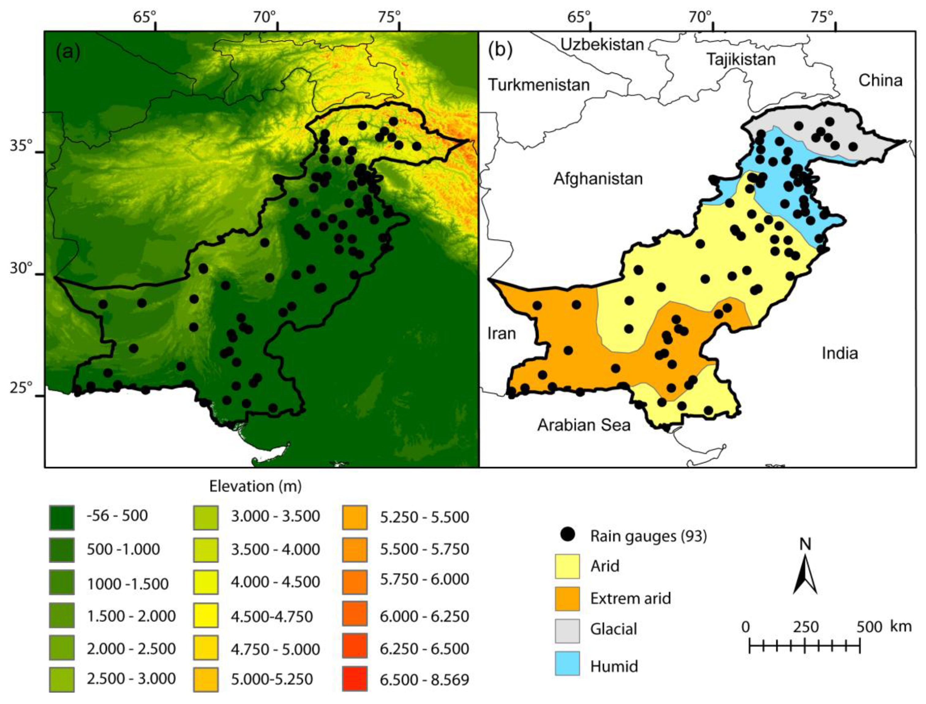
2.1. Study Area

Pakistan is situated in the western zone of South Asia between 23.5–37.5°N latitude and 60–78°E longitude. Geographically, it is bounded at north by China, east by India, while Afghanistan and Iran cover the western side. Arabian Sea marks the southern border (Figure 1). The total area is 803,940 km2 where elevation as varies from a maximum of 8011 m at K2 (second elevated peak on earth) to about 0 m at the Arabian Sea. Climatologically, the study area is very diverse in space and time, and it is divided into different climatic zones [34]. For the present study, four regions are considered to assess SPEs performance over variable geomorphic and meteorological contexts (Table 1).
The glacial region is located at the extreme northern edge of Pakistan having mean elevation of about 4158 m. It is mostly covered with glaciers and permanent snow. The summer snow melting contributes to the rivers flowing and is used as a source of agriculture in the country. Excessive snow melts and under ice streams can cause flooding in the lower elevated areas [35].
The humid region includes very high mountains of the Hindukush, Karakoram, and Himalaya (HKH) regions and all major rivers of Pakistan rivers (Indus, Kabul, Swat, Chitral, Gilgit, Hunza, Kurram, Jhelum, and Panjkora) originate from these regions. The region is located at a mean elevation of 1286 m and it counts with the highest precipitation amount estimated as 852 mm/year.
The arid region is characterized by low–lying plains consisting in the major agriculture regions (Punjab plain) that are drained by the Indus River and its tributaries [35]. The region counts with an average elevation and annual rainfall of 633 m and 322 mm/year, respectively.
The extreme arid region consists in barren lands located at the southern end of the country towards Arabian Sea and Iran. There are low dry mountain ranges with a mean average elevation of 444 m and very low amount of precipitation estimated as 133 mm/year

2.2. Datasets

2.2.1. GPM Based Satellite Precipitation Estimates

IMERG is a product of the National Aeronautics and Space Administration (NASA). It uses both passive microwave (PMW) and infra–red (IR) sensors available from Low Earth Orbital (LEO) and geostationary satellites, respectively. First, precipitation estimates that were derived from PMW datasets while using the Goddard Profiling algorithm (GPROF) are calibrated (i) to the GPM Combined Radar-Radiometer (CORRA) precipitation estimates that were derived from GPM Microwave Imager (GMI) and Dual-Frequency Precipitation Radar (DPR) and (ii) to the Precipitation Climatology Centre (GPCP) monthly precipitation estimates. Then, the PMW precipitation estimates are blended using the CMORPH–Kalman Filter (CMORPH–KF) Lagrangian time interpolation and the Precipitation Estimation from Remotely Sensed Information using Artificial Neural Networks–Cloud Classification System (PERSIANN–CSS). The blending process relies on motion vectors derived from the Climate Prediction Center IR (CPC–IR) cloud top temperature to produce half hourly precipitation estimates.
The IMERG system is run twice to produce the IMERG Early, Late and Final run product at 4 h, 12 h, and 2.5 month after observation time, respectively. Because of the availability at short latency, the 45-day interval CORRA, the 30-day interval PERSIANN-CSS, and the three-month interval CMORPH-KF interpolation calibrations steps are necessarily trailing for the Early and Late runs, whereas a centered approach is used for the Final run. Ancillary products required on routine basis for IMERG algorithm also change according to the considered version (Early, Late, Final). Required data of surface temperature, relative humidity and surface pressure are provided by the Japanese Meteorological Agency (JMA), the GANAL gridded assimilation, and the European Centre for Medium-range Weather Forecasting (ECMWF) for the Early, Late, and Final run, respectively. Finally, the post processing adjustment step involved climatological based coefficient to produce the Early and Late run product while Global Precipitation Climatology Project (GPCC) monthly precipitation gauge analysis based coefficients are used to produce the Final run product. For more information on IMERG processing, please refer to [36].
From the year 2014 to 2018, three successive IMERG versions were made available. IMERG–v03 was the first version released in 2014, followed by IMERG–v04 in 2017, and then IMERG–v05 in early 2018. The main change among IMERG–v03, –v04, and –v05 rely on the use of successively different GPROF algorithm versions (GPROF–v03, –v04, and –v05). Differently to GPROF–v03, GPROF–v04 and –v05 used threshold precipitations rate to adjust fractional coverage. Others changes from IMERG–v03 to –v04 (and –v05) are: (1) the use of Global Precipitation Climatology Project (GPCP) v2.3 to compensate for the GPM combined instrument dataset (2BCMD) bias over non tropical oceans and land; (2) inclusion of the Advanced Technology microwave Sounder (ATMS) dataset; (3) dynamic calibration of PERSIANN–CSS by PMW derived precipitation estimates; (4) increase in HQ precipitation field spatial coverage from 60°N–S to 90°N–S; and, (5) removal of the GPCC grid box volume adjustment to eliminate blocky gauge adjustment (Final run only). The benefit of blocky gauge adjustment is clearly observable in Figure 2 with the total removed of blocky effects from IMERG–v03 to IMERG–v04 and –v05. Main changes in IMERG–v05 in comparison to previous –v04 and –v03 versions include some restrictions in Microwave Humidity Sounder (MHS) and ATMS swaths (for the five and eight footprints, respectively) and the no-consideration of TRMM Microwave Imager (TMI). For the present study, we used the IMERG–v03, –v04, and –v05 Final run.
GSMaP is a product of the Japan Science and Technology (JST) agency under the Core Research for Evolutional Science and Technology (CREST). Its precipitation estimates are based on PMW and IR datasets combination. In the first step, the precipitation estimates are derived from PMWs brightness temperature [37]. Then, a Kalman filter model is used to refine the precipitation rate propagated using the atmospheric moving vector derived from CPC–IR data [38], providing hourly precipitation estimates. The resultant product, GSMaP–MVK, is finally calibrated using the CPC unified gauge–based analysis of global daily precipitation. It is worth mentioning that GSMaP–MVK is available three days after observation time. To reduce data latency, a near real time version (GSMaP–NRT) using simplification in the processing is made available three hours after observation.
From 2014 to 2018, two successive versions of GSMaP were made available. The GSMaP–v06 was the first version released in 2015 and followed by GSMaP–v07 in 2017. The main modifications from GSMaP–v06 to GSMaP–v07 algorithm are: (1) the use of GPM/DPR observation as database; (2) implementation of snowfall estimation over high latitudes; and, (3) improvement of (i) gauge–calibration, (ii) orographic rain correction method, and (iii) weak precipitation detection over the ocean. For the present study, we only consider GSMaP–v06 and –v07 gauges adjusted versions (MVK).

2.2.2. TRMM Based Satellite Precipitation Estimates

Climate Prediction Center Morping (CMORPH) is a product of NOAA/CPC. Precipitation estimates are derived from PMW datasets and propagated in space and time while using a motion vector derived from CPC–IR data [2]. Recently, CMORPH was reprocessed using a fixed algorithm and homogeneous input to fix substantial inconsistencies in its first version between 2003 and 2006. The new version (CMORPH–v1.0) covers the entire period 1998 to the present, whereas the first version’s (CMORPH–v0x) coverage started in 2002. There is an only satellite based version (CMORPH–RAW), a bias corrected version (CMORPH–CRT), and a satellite gauge blended version (CMORPH–BLD). CMORPH–CRT is derived from CMORPH–RAW adjustment while using the CPC unified gauge-based analysis over land and the pentad GPCP over the ocean [39]. CMORPH–CRT is then combined with the gauge analysis through the optimal interpolation technique to generate CMORPH–BLD [40]. For the present study, we consider CMORPH–CRT and –BLD. The choice is based on recent study in which CMORPH–CRT was found to outperform CMORPH–RAW [35]. As CMORPH–BLD is derived after an adjustment made to CMORPH–CRT, it is naturally selected to highlight potential benefit from the adjustment process.
TRMM Multisatellite Precipitation Analysis (TMPA) is a product of NASA in collaboration with the JAXA. Precipitation estimates are derived from PMW datasets and gaps are filled using CPC–IR, Meteorological Operational satellite program (MetOp), and GridSat–B1 datasets [1]. TMPA–v07 is the last available TMPA version since its predecessor (TMPA–v06) ended in July 2011. Enhancement form –v06 to –v07 version came from the consideration of a larger amount of PMW and IR data. It has a satellite based version (TMPA–RT) and a gauges adjusted version (TMPA–Adj). The TMPA–Adj version is derived from TMPA–RT adjustment using GPCP and Climate Assessment and Monitoring System (CAMS) datasets [1]. For the present study, we only consider the TMPA–Adj as it was found to outperform TMPA–RT version over Pakistan [35].

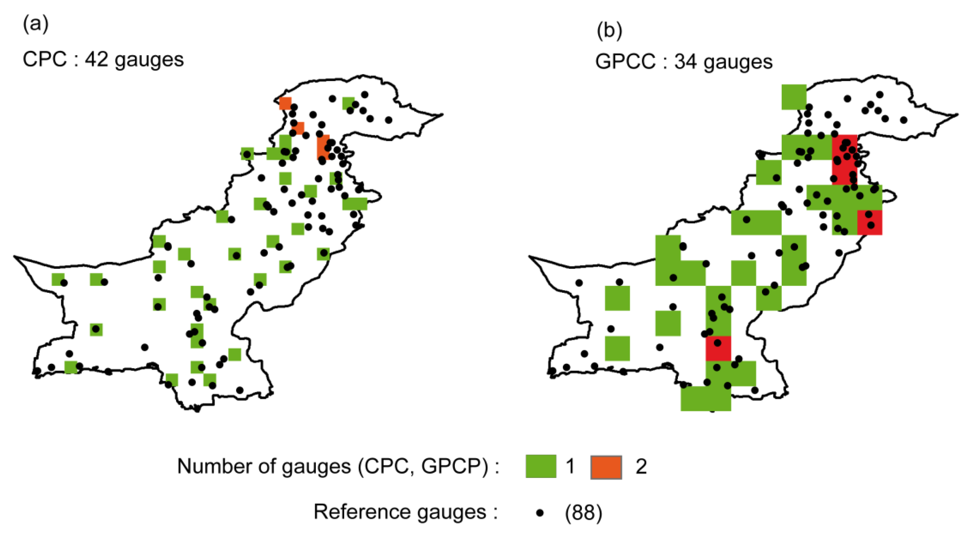
2.2.3. Gauges Precipitation Data

Meteorological data of Pakistan is owned by different organizations, such as Pakistan Meteorological Department (PMD), Water and Power Development Authority (WAPDA) of Pakistan, University of Boon under the Culture Areas Karakoram (CAK) program in the Bagrot valley and Yasin catchment of Gilgit basin during 1990–91, and Ev-K2-CNR (an Italian based organization). However, for the present, only the data handled by the PMD at 88 stations over one year period (1 January–31 December 2015) was made available and used. The data are manually collected and therefore subject to error introduce by personnel and instrumental errors. Additional errors for the gauges that are located in high elevation regions come from the wind effect, which might bias the precipitation collection by the gauges. In this context, the PMD follows the World Meteorological Organization (WMO) standard code WMO-N for the evaluation and correction of gauge-based precipitation data [41] to ensure as consistency as possible in the measurements. Therefore, the provided precipitation data by PMD were considered as ground truth for evaluation of the SPEs.
The dataset spread over the considered regions with 8, 26, 32, and 22 gauges for the glacial, humid, arid, and extreme arid regions, respectively (Table 1). Some of the stations located in the mountainous northern region (glacial and humid region) count with snowfall events. For these specific stations, the recorded snowfall is melted with hot water. Then, the hot water volume is removed from the total water (snowfall + hot water) to retrieve the snowfall water equivalent.
Finally, Figure 3 shows the Global Precipitation Climatology Project (GPCC) and Climate Prediction Center (CPC) gauges network used for the monthly and daily gauges based precipitation grid for the SPEs adjustment over the 2015 year. It is worth mentioning that both GPCP and CPC share common gauges with the gauges network that is used as reference in the present study. Therefore, the gauges network that was used for the SPEs assessment is not totally independent of the assessed SPEs and could influence SPEs performances conclusions. It is worth mentioning that Figure 3 aims at providing a general overview of potential overlapping between the reference gauge network with both CPC and GPCC one. Indeed, gauges from the other above-mentioned organizations might also be part of the CPC and GPCC gauges network.

2.3. Method Used

2.3.1. SPEs and Gauges Pre-Processing

For the inter-comparison of CMORPH–CRT, –BLD, and TMPA with IMERG–v03, –v04, –v05 and GSMaP–v06 –v07, all IMERG and GSMaP datasets were first resampled from their original grid size (0.1°) to the CMORPHs and TMPA grid size (0.25°), according to the protocol that was proposed by [15]. To do so, IMERG and GSMaP were first resampled from 0.1° to 0.05° grid scale and the precipitation at the 0.25° grid is obtained by taking the mean precipitation value of the 25 pixels (0.05°) included into the 0.25° pixel.
For each of the grid box (0.1° and 0.25°), including gauges, daily temporal records are computed from all SPEs using 8 h to 8 h (local time) temporal windows to match with daily gauges observations. Then, monthly records are computed from daily records only for the month with more than 80% of available daily records for all SPEs and the gauges. Figure 4 shows the percentage of available daily and monthly values at each pixels location. To ensure robustness in the analysis, the database used for the SPEs assessment only considered stations with more than 90% of available data over the considered period (1 January–31 December 2015).
Finally, mean regional daily and monthly records are computed for the entire Pakistan, glacial, humid, arid, and extreme arid regions from the gauges ( P r e f ) and all SPEs by aggregating the records from all of the pixels (including gauges) included in the considered region.

2.3.2. SPEs against Gauges at the Monthly Time Step

First, for each region (entire Pakistan, glacial, humid, arid, and extreme arid) SPEs mean monthly regional series were compared to the gauges in terms of Correlation Coefficient (CC), Standard Deviation (STD), Centered Root Mean Square Error (CRMSE), and percentage Bias (%B) (Equations (1)–(4)).
C C = C o v ( S P E , P r e f ) S T D S P E × S T D r e f
where CC is the correlation coefficient, SPE and Pref are the SPE and Pref precipitation time series, and Cov is the covariance.
S T D = 1 n i = 1 n ( P i P ¯ ) 2
where STD is the standard deviation in mm, n is the number of values, and P the precipitation value in mm (SPE or Pref).
% B = 1 n i = 1 n ( S P E i P r e f i ) 1 n i = 1 n P r e f i × 100
where %B is the SPE Bias value in percentage, n is the number of values; SPE the precipitation estimate of the considered SPE value in mm, and P r e f the reference precipitation value in mm.
C R M S E = 1 n i = 1 n ( ( S P E i S P E ¯ ) ( P r e f i P ¯ r e f ) ) 2
where CRMSE is the centered root mean square error in mm, n is the number of values, SPE the precipitation estimate of the considered SPE value in mm, and Pref the reference precipitation value in mm.
To facilitate the inter-comparison among all considered SPEs, the results are presented in the form of Taylor diagram [42]. Taylor diagram consists in an integrated graphical representation of CC and normalized STD and CRMSE values. STD and CRMSE are normalized by dividing SPEs STD and CRMSE by Pref STD. In this context, SPEs optimum statistic scores are reached for CC, STD, and CRMSE values equal to 1, 1, and 0, respectively (Pref score). Therefore, in the Taylor diagram, the closest is the SPEs to the reference dot the closest are the SPEs and Pref estimates. Additionally, %B is considered to observe SPEs potential over/underestimation.
Secondly, CRMSE is computed at the pixel level (including gauges) for all SPEs and are plotted to observe very local SPEs performance at the pixel scale. Only CRMSE is considered as it consists in the most discriminating statistical scores. Indeed, in the Taylor diagram, CRMSE constrained SPEs relative position to the dot reference. %B is also computed and plotted to observe SPEs potential over/underestimation spatial variability.

2.3.3. SPEs against Gauges at the Daily Time Step

The daily performance assessment is based on categorical statistics aiming at measuring SPEs capacity for the detection of daily precipitation events. The statistics are based on a contingency table considering daily precipitation as a discrete value with two possible cases: day with or without precipitation (Table 2).
Four indexes are considered: the Probability of Detection (POD), the False Alarm Ratio (FAR), Critical Success Ratio (CSI) the Bias, and the Heidke Skill Score (HSS) (Equations (5)–(9)).
P O D = a ( a + c )
F A R = b ( a + b )
C S I = a ( a + b + c )
B i a s = ( a + b ) ( a + c )
H S S = 2 ( a d b c ) [ ( a + c ) ( c + d ) + ( a + b ) ( b + d ) ]
POD aims at representing SPE’s ability to correctly forecast precipitation events. Values vary from 0 to 1, with 1 as a perfect score.
FAR aims at representing how often SPE detect precipitation event, when, actually, it does not occur. Values vary from 0 to 1, with 0 as a perfect score. FAR is also represented in form of the Success Ratio (SR = 1 − FAR).
CSI is the ratio between the number of precipitation events that are correctly detected by the SPE and the number of all precipitation events, as registered by the gauge and the SPE. Values vary between 0 and 1 with a perfect score of 1.
Bias aims at representing SPEs tendency to under forecast (Bias < 1) or over forecast (Bias > 1) precipitation events with a perfect score of 1.
HSS consists in a generalized skill score on precipitation events forecasting compared to a random based prediction. Values range from −∞ to 1 with a perfect score of 1 and negative values indicating that the random based prediction outperforms the SPE one.
POD, SR, CSI and Bias are computed for all SPEs and considered regions (entire Pakistan, glacial, humid, arid, and extreme arid) from the respective mean regional daily precipitation series while using a threshold value of 1 mm/day to differentiate precipitation to no precipitation events [15,24]. It is worth mentioning that some authors used an increasing threshold to assess SPEs performance for different precipitation intensities (e.g., [43,44,45]). However, for the present study, most of the assessed pixels count with only one gauge. Therefore, the representativeness between areal (SPE pixel) and point (gauges) measurement should decrease with increase in threshold value.
To facilitate SPEs inter-comparison, results are presented in form of a performance diagram [45]. The performance diagram integrates POD, SR, CSI, and Bias in a geometric way in which the relative position of the reference dot located in the upper left corner permits the SPEs performance inter-comparison. The reference dot corresponds to POD, SR, CSI, and Bias values of 1, 0, 1, and 1, respectively. Closer is the SPE to the reference dot, higher are the SPEs forecasting ability.
Finally, HSS is computed at the pixel level (including gauges) for all SPEs and are plotted to observe very local SPEs potential in daily precipitation event forecasting ability.

2.3.4. Benefits of GPM Based SPEs Successive Versions

The objective of this section is to have first insight into the potential benefits of the successive GSMaP and IMERG versions at the monthly scale.
For each pixel including gauges, the GSMaP versions (–v06 or –v07) with the lowest CRMSE being plotted to localize the most suited version in space. Additionally, the absolute CRMSE difference between the two versions are also plotted to quantify the spatial enhancement between both versions.
Similarly, for each pixel including gauges, the IMERG versions (–v03, –v04, –v05) with the lowest CRMSE are also plotted. Because three versions are available for IMERG estimates, the absolute CRMSE difference is based on the versions with the highest and lowest CRMSE values.

2.3.5. Benefits of GPM over TRMM Based SPEs

This section aims at presenting which SPEs between GPM and TRMM considered in this study provides the most accurate precipitation estimates over Pakistan. At each gauge location, the SPEs with the lowest CRMSE and %B are plotted to highlight the SPE that should be used for the specific pixel location.

3. Results

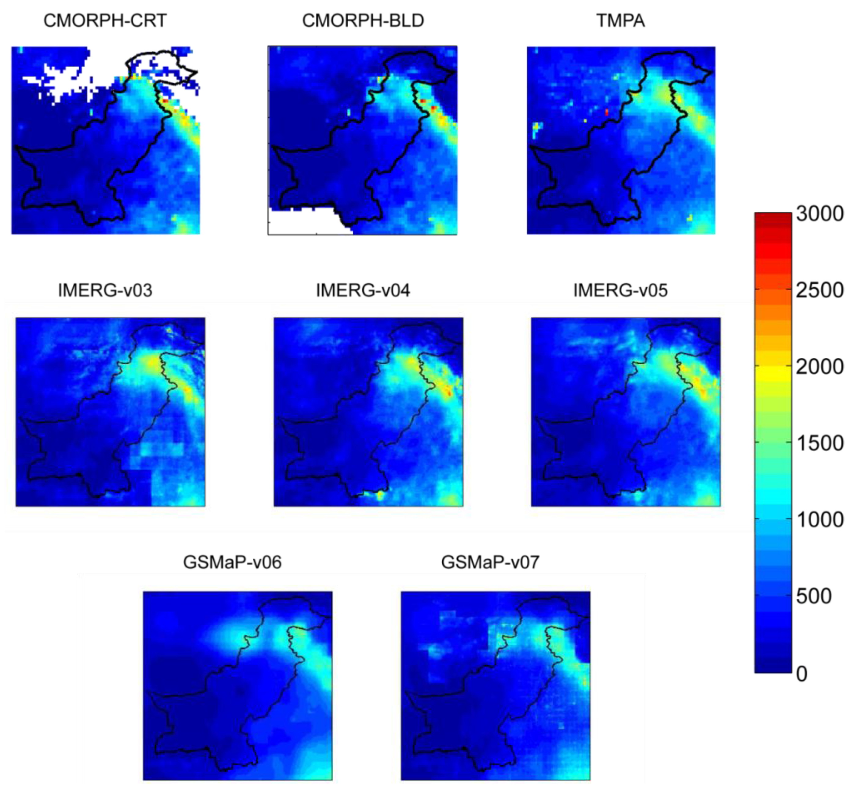
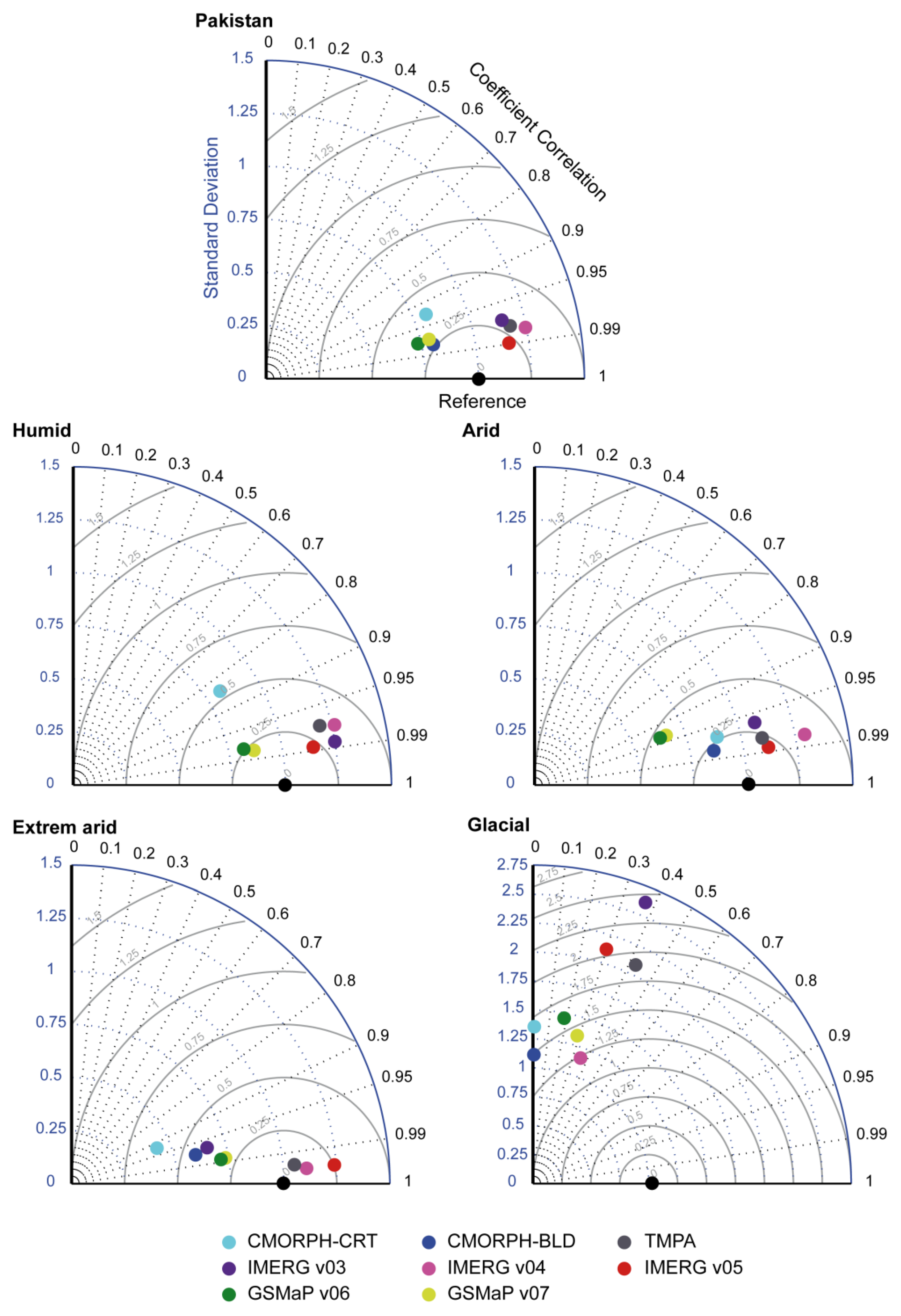
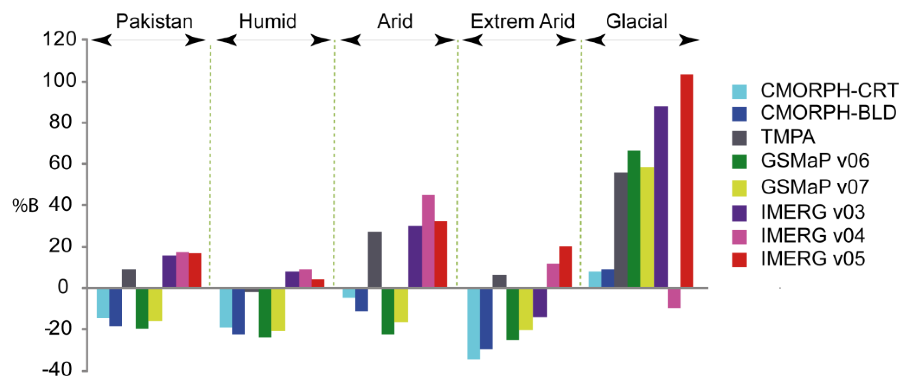
3.1. SPEs Monthly Performance at the Regional Scale

Figure 5 shows the SPEs performance for each considered regions in the form of Taylor diagram. On a general way, all SPEs provide relatively accurate precipitation estimates over the entire Pakistan, humid, arid, and extreme arid regions with CRMSE lower than 0.5 and CC higher than 0.9. On the contrary, all the SPEs performances are very low over the glacial region with CRMSE higher than 0.5 and CC lower than 0.5.
When considering the GSMaP versions, the new released GSMaP–v07 always provide closer estimates to the reference in comparisons to the previous GSMaP–v06.
Regarding to IMERG versions, the enhancement from successive versions are more contrasted. Indeed, IMERG–v05 precipitation estimates are closer to the reference for the entire Pakistan, humid and arid regions with CRMSE value of approximately 0.2 for all of the regions. However, over the extreme arid region, IMERG–v04 is found better than IMERG–v05. A similar inconsistency is observable over the humid and arid regions with IMERG–v03 closer to the reference than IMERG–v04.
When compared to the TRMM based SPEs versions (CMORPH–CRT, CMORPH–BLD, and TMPA), the benefit of the new GPM based SPEs (IMERG and GSMaP) is not evident. When considering the entire Pakistan, CMORPH–BLD estimates performance (CRMSE = 0.26) is closer to GSMaP–v07 (CRMSE = 0.29) and IMERG–v05 (CRMSE = 0.21). The same is true for the humid region. Over the arid region, GSMaP–v06 and –v07 are outperformed by TRMM based SPEs, while IMERG–v05 still provides more accurate precipitation estimates (CRMSE = 0.19). Finally, for the extreme arid region, TMPA (CRMSE = 0.1) outperformed all GPM based SPEs.
Figure 6 shows the %B observed for all SPEs over the different considered regions. Regarding GSMaP–v06 and –v07, they both underestimate precipitation for the entire of Pakistan, humid, arid, and extreme arid regions with %B around −20% and highly overestimate precipitation over the glacial region. Overall, GSMaP–v07 is slightly less biased than GSMaP–v06.
Regarding IMERG–v03, –v04, and –v05, the opposite trend is observed for the entire Pakistan, humid, arid, and extreme arid as they all overestimate the precipitation. For all IMERG versions, the %B is around 5% for the humid region and superior to 30% for the arid region. For the glacial region, IMERG–v03 and IMERG–v05 highly overestimate the precipitation estimates with %B superior to 80% and 100%, respectively, while IMERG–v04 is the less biased (absolute %B < 15%) product among GPM based SPEs.
TMPA %B is very low for the entire Pakistan, humid and extreme arid regions with respective values of 9%, −2%, and 6%, while it considerably overestimates precipitation over the arid and glacial regions with %B of 27% and 56%.
Similar to GSMaP–v06 and –v07, CMORPH–CRT and CMORPH–BLD underestimate precipitation over the entire Pakistan, humid, arid, and extreme arid regions. The bias is very low and very high for the arid and extreme arid regions, respectively. Interestingly, unlike the other SPEs, CMORPH–CRT, and BLD present %B lower than 10% over the glacial region.

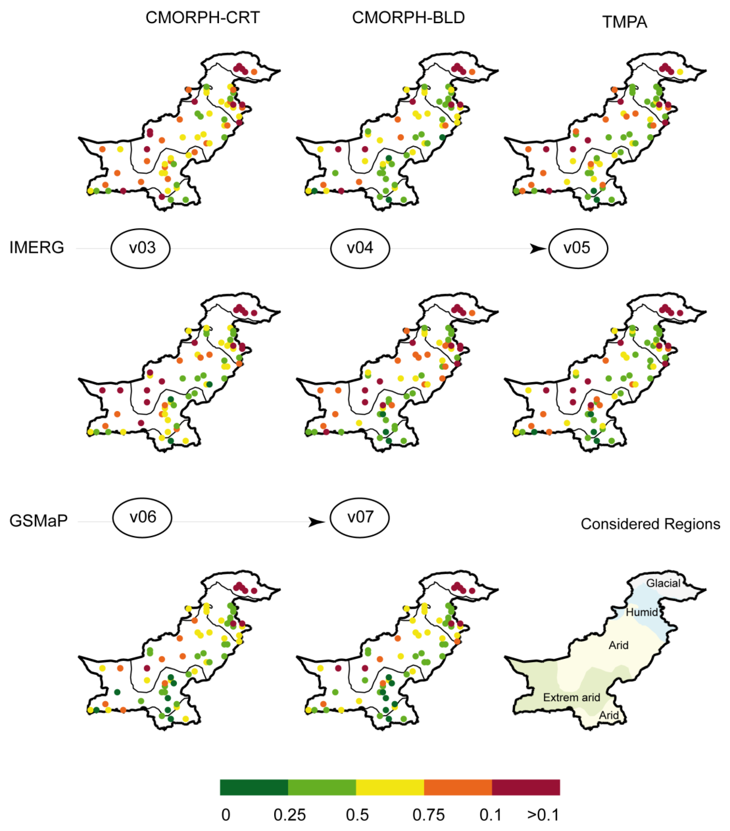
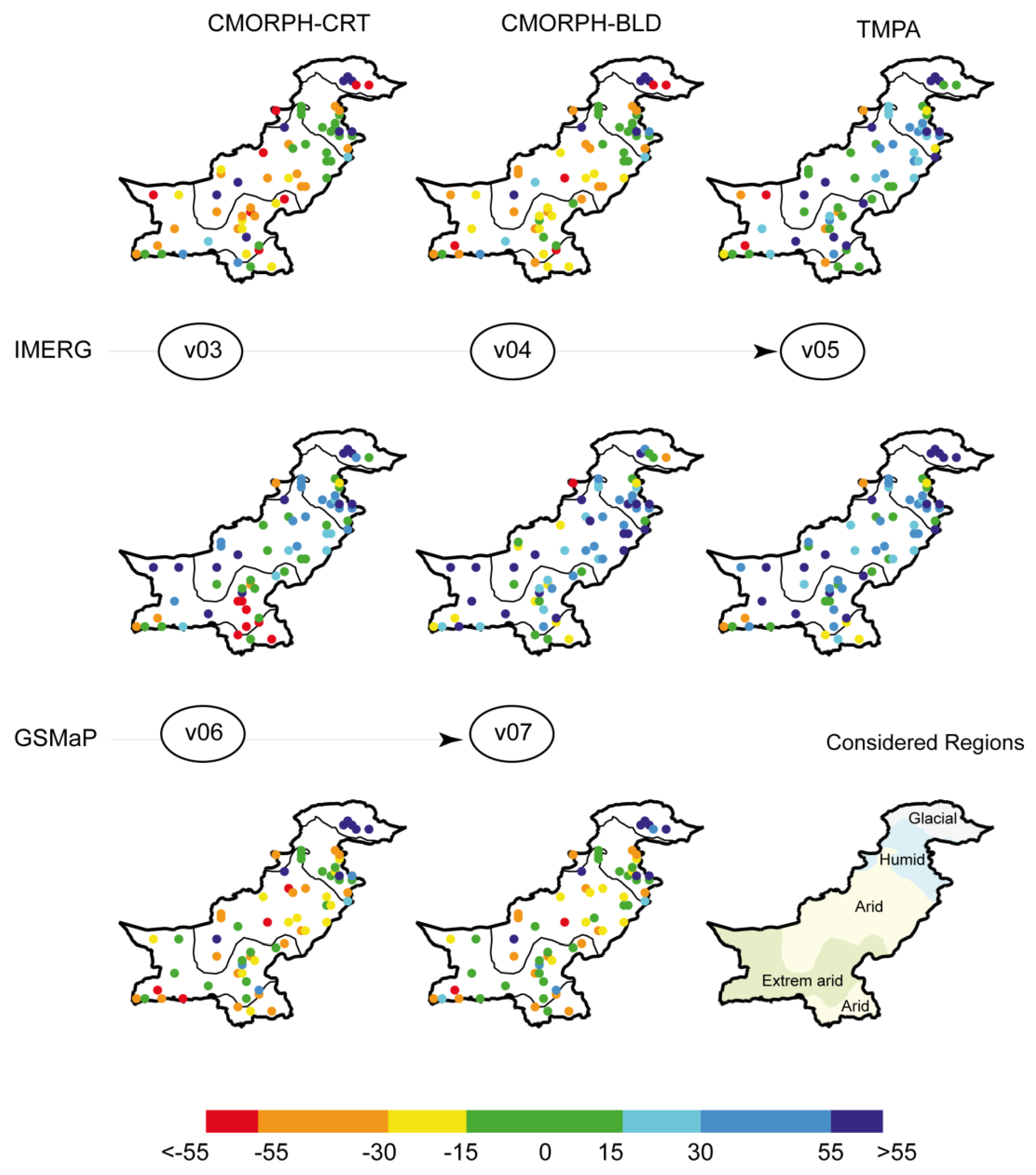
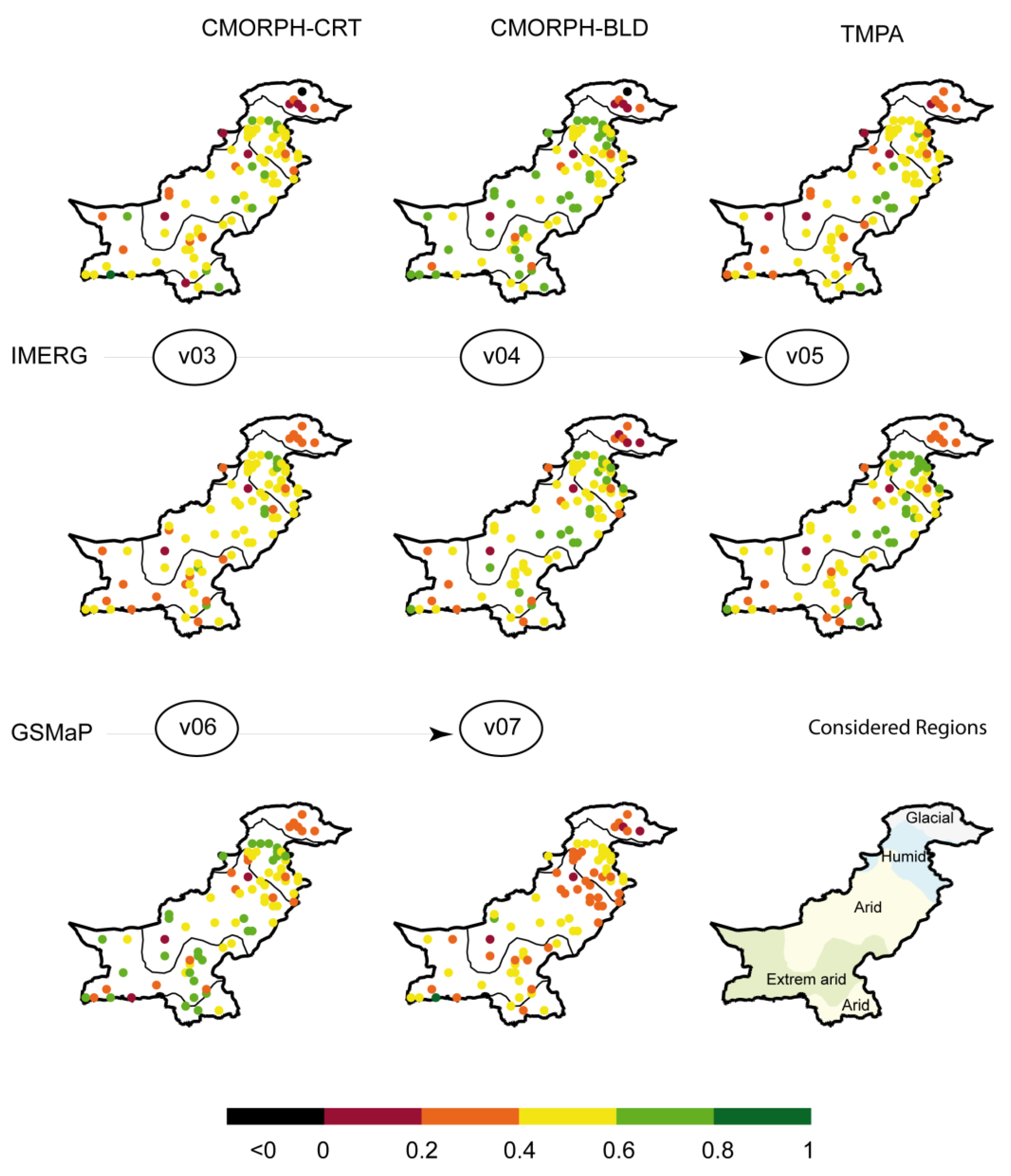
3.2. SPEs Monthly Performance at the Gauge scale

Figure 7 shows the CRMSE obtained for each pixel including gauges at the monthly time step. CRMSE value is selected as it controls SPEs relative position in the Taylor diagram, and therefore can be used easily for the evaluation of inter-comparative performance of SPEs. All SPEs are better able to represent precipitation spatial variability in the eastern than western part in the arid and extremely arid regions. All SPEs performance is very low over the northern glacial region with CRMSE value higher than 1.
Among TRMM based SPEs, the enhancement from CMORPH–CRT to CMORPH–BLD is observable over the extreme arid and humid regions with an overall increase in the number of pixel with CRMSE value lower than 0.5 (almost three times as many). TMPA presents a quite similar CRMSE pattern than CMORPH–BLD, except over the arid region where CMORPH–BLD has better captured the precipitation spatial variability with higher proportion of pixels with CRMSE values lower than 0.5.
When considering the IMERG successive versions (–v03, –v04, –v05), a high discrepancy is observed in their respective ability to represent the precipitation spatial variability. The most suitable version (in term of CRMSE values) changes along the considered regions. IMERG–v04 has the highest number (13) of pixel with CRMSE lower than 0.5 over the extreme arid region in comparison to IMERG–v03 (7) and –v05 (9). Over the arid and humid regions, the lastest released IMERG–v05 outperformed its previous versions (IMERG–v03, –v04) with many pixels having a CRMSE value lower than 0.5. However, over the glacial region, all IMERG versions perform very poorly with unsatisfactory CRMSE values systematically higher than 0.5.
When considering the GSMaP SPEs successive versions (–v06, –v07), the error spatial distribution in the form of CRMSE values are very close over the entire Pakistan, irrespective of the considered region. Both versions performed very poorly over the glacial region with a CRMSE value higher than 1.
Figure 8 shows the %B that was obtained for each pixel, including gauges, at the monthly time step. CMORPH–CRT and CMORPH–BLD present very similar %B distribution with relatively low %B value and many pixels in the −15% to 15% ranges over the humid and northern arid regions. Besides, at the regional scale they both tend to underestimate monthly precipitation with a dominant proportion of pixels with negative %B values. Over the glacial region, CMORPH products strongly overestimate (underestimate) precipitation for the western (eastern) located pixels. On the contrary, TMPA tends to overestimate monthly precipitation over the entire of Pakistan, especially over the humid and northern arid regions. The pixels with −15% to 15% (%B) ranges are mainly located in the central Pakistan over the arid and extreme arid regions. Over the glacial region, TMPA strongly overestimates precipitation for the western located pixels, whereas reasonable %B values are found for the two eastern located pixels.
Regarding IMERG successive versions (–v03, –v04, –v05), they all tend to overestimate monthly precipitation at the regional scale. The %B pattern is very close for all IMERG versions over the humid region. Differences account over the arid region, where IMERG–v03 presents the highest number of pixel (7), with %B values ranging from −15% to 15%. Interestingly, for the pixels that are located southeast, the strong positive %B for the first IMERG version (IMERG–v03) was consistently corrected for the following IMERG versions (–v04, –v05). Over the glacial region, IMERG–v04 presents the lowest %B values in comparison to its previous (–v03) and following (–v05) versions.
Similar to the CRMSE values, GSMaP–v06 and –v07 present very close %B spatial distribution with an overall trend of underestimation of the monthly precipitation. Pixels, with %B ranging from −15% to 15%, are mainly located over the extreme arid and humid regions. As observed for TRMM based SPEs and IMERG datasets, GSMaP–v06 and –v07 %B are very high for the pixels that are located in the glacial region.

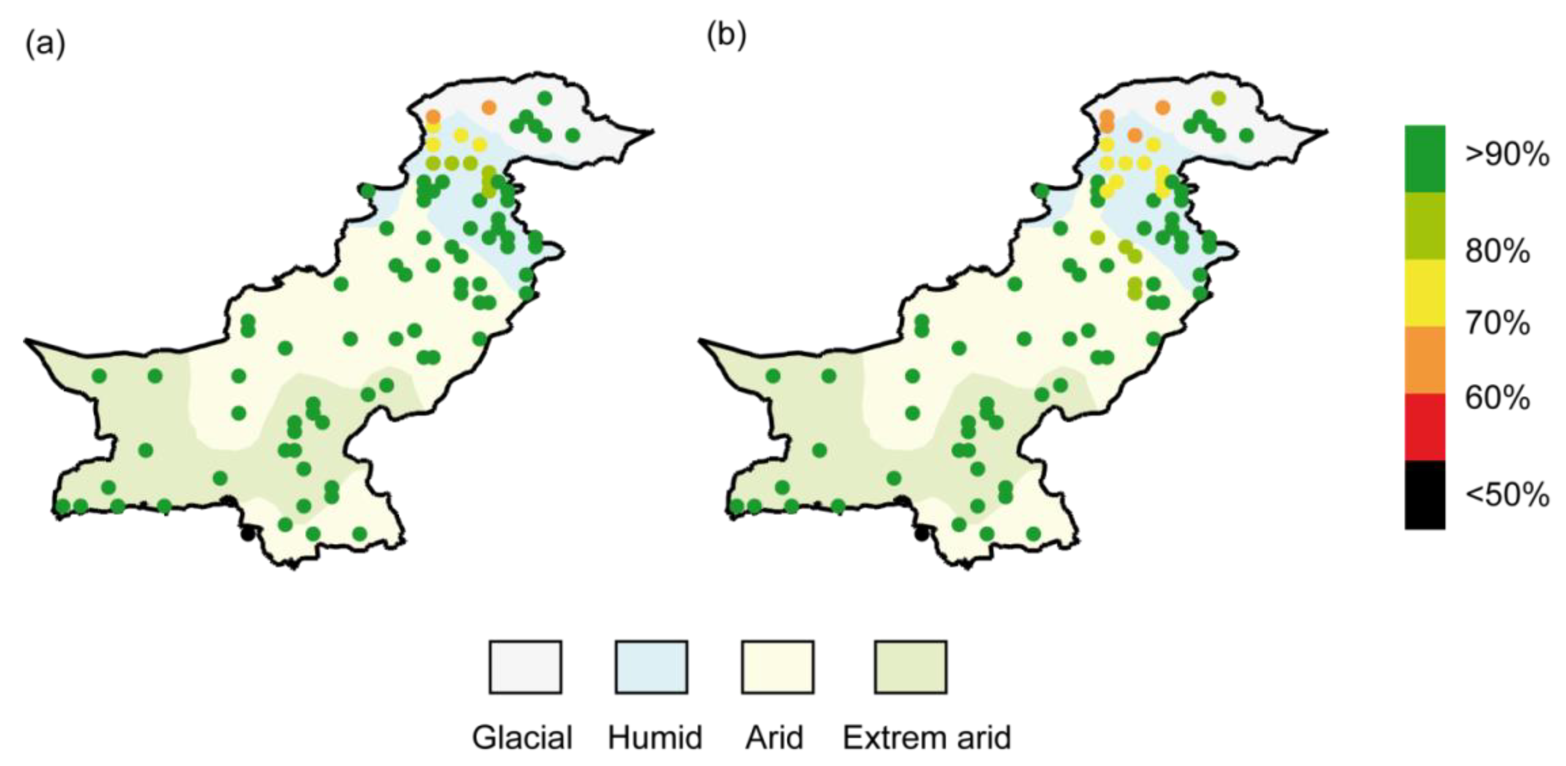
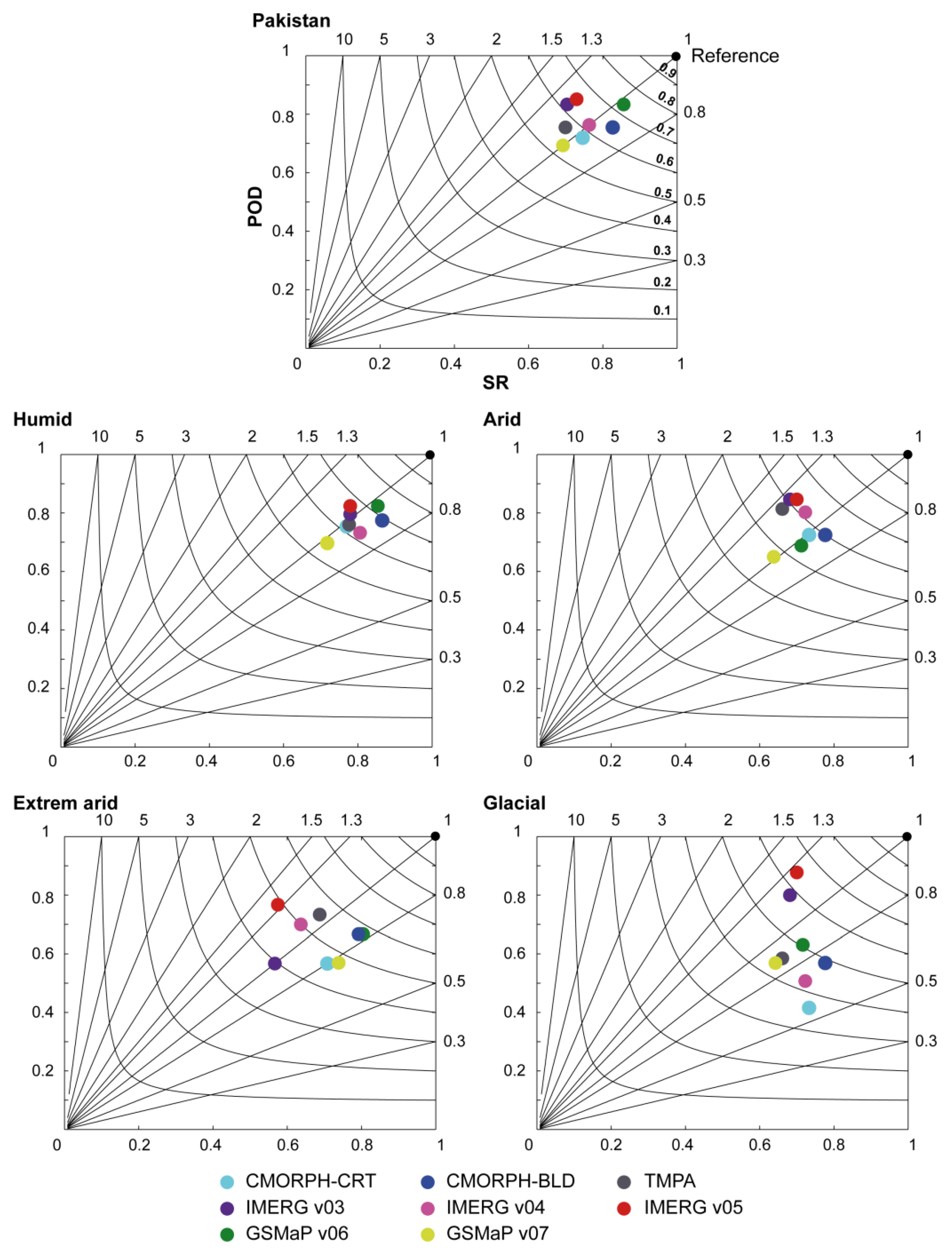
3.3. SPEs Daily Potential at the Regional Scale

Figure 9 shows the SPEs daily precipitation events forecasting ability for the entire Pakistan and each considered regions in the form of performance diagram. On a general way, SPEs performance at the daily time step is higher for humid and arid regions than for the extreme arid and glacial regions. SPEs performances are closer for the humid and arid region with a close relative position in the performance diagram than for the extreme arid and glacial regions.
When considering the TRMM based SPEs, CMORPH–BLD performance is highest than its non-gauges adjusted version CMORPH–CRT. Indeed for all regions, CMORPH–BLD is found to be closest to the reference dot. This shift is induced by an increase of SR over the entire Pakistan, humid and arid regions, whereas an increase of POD also contributes to CMORPH–BLD enhancement over the extreme arid and glacial regions. In comparison to TMPA, CMORPH–BLD presents the highest ability for daily precipitation events forecasting for all considered regions.
When considering the three successive IMERG versions, their performances for the entire Pakistan are close with IMERG–v05 slightly closer to the reference dot. Similar observation is true for the humid and arid regions where IMERG–v05 outperformed its two previously released versions (–v03 and –v04). Much variability in IMERG relative performance is observable over the extreme arid and glacial regions with IMERG–v04 (–v05) performing better over the extreme arid (glacial) regions.
Interestingly, for all considered regions, GSMaP–v07 is less able to forecast daily precipitation event than it previous version (GSMaP–v06). Indeed, from GSMaP–v06 to –v07 a decrease is observed in all considered indexes (POD, SR, CSI and Bias). GSMaP–v06 outperformed all considered SPEs at the daily time step for the entire Pakistan, humid and extreme arid regions.

3.4. SPEs Daily Potential at the Gauges Scale

Figure 10 shows the SPEs spatial consistency at the daily time step expressed in the form of HSS. From all the considered TRMM based SPEs, CMORPH–BLD is far from the SPEs with the highest ability for daily precipitation events forecasting. It has the highest number of pixels with HSS that is higher than 0.6 homogeneously distributed all over the Pakistan. However, its performance is particularly bad over the glacial regions as illustrated by the top northern located pixel with a negative HSS value.
Contrary to the observation made for the monthly time step, the successive IMERG versions consist in a continuously improvement in daily precipitation event forecasting. Indeed, the number of pixels with HSS higher than 0.6 considerably increased from IMERG–v03 to –v04 (especially over the arid region) and slightly increased from IMERG–v04 to –v05. However, over the glacial regions, the HSS is low (HSS < 0.4) for all pixels and considered IMERG versions.
When considering the GSMaP–v06 and –v07 versions, the first GSMaP version (–v06) presents the highest number of pixels with HSS higher than 0.6, confirming the observation that is presented in Figure 9. It is clearly observable over the humid and extreme arid regions. As observed for TRMM based SPEs and IMERG datasets, GSMaP–v06 and –07 performance are very low over the glacial region (HSS < 0.4).

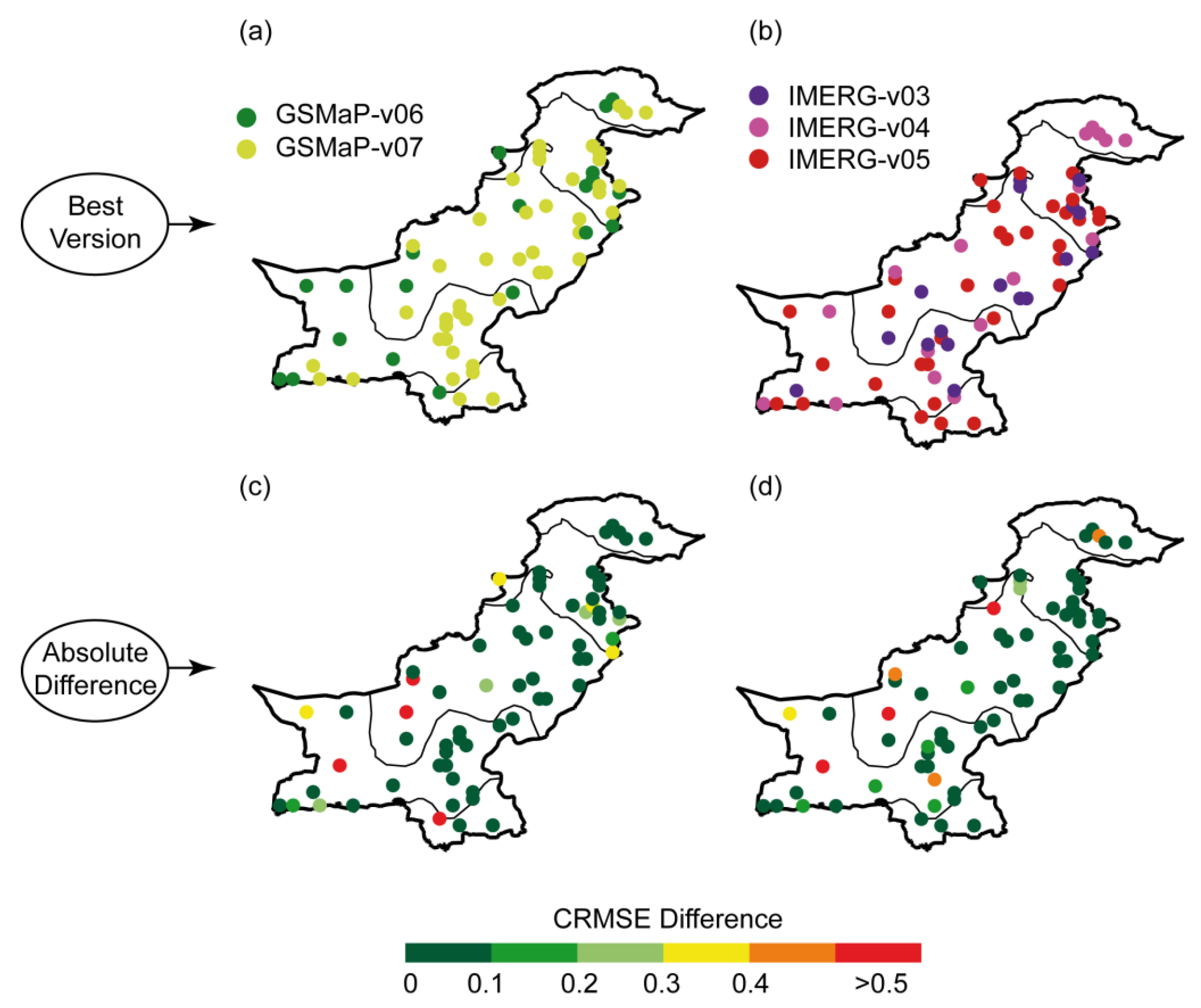
3.5. Benefits of GPM Based SPEs Successive Versions

Figure 11 shows GSMaP and IMERG most suited version at each gauges location, according to the CRMSE values. Additionally, the absolute CRMSE difference between the most and least suited version is given to quantify the potential enhancement of successive versions.
Regarding GSMaP successive versions, GSMaP–v07 is the most accurate version with lowest CRMSE value obtained at most of the gauges location. It is worth mentioning that for all pixels where GSMaP–v07 performed better than GSMaP–v06, the difference in CRMSE value is very low (<0.1), meaning that both versions performed quite similarly at those pixels location. However, for the pixels where GSMaP–v06 outperforms GSMaP–v07, CRMSE difference is much higher with differences that are higher than 0.5 in the arid and extreme arid regions. Therefore, the enhancement of GSMap–v07 is not very efficient and brought local inconsistency, especially over the arid and extreme arid regions.
When considering IMERG successive versions, the last IMERG–v05 is the most efficient with the highest numbers of pixels (32), where it outperformed its previous versions IMERG–v03 and IMERG–v04. Both IMERG–v03 and –v04 count with 17 pixels where they provide the best monthly precipitation estimates. IMERG–v04 (–v05) is the most efficient to capture precipitation variability over the glacial (arid) region, confirming previous results at the regional scale (Figure 5). However, the absolute difference in CRMSE values is very low overall (<0.1), meaning that all versions performed quite similarly over the Pakistan. Interestingly, the pixels with the highest absolute difference in CRMSE value (>0.5) account for the pixels where the last IMERG–v05 provides the best monthly precipitation estimates. This shows the benefits that are brought by the last IMERG–v05 over the previously released IMERG–v03 and –v04.

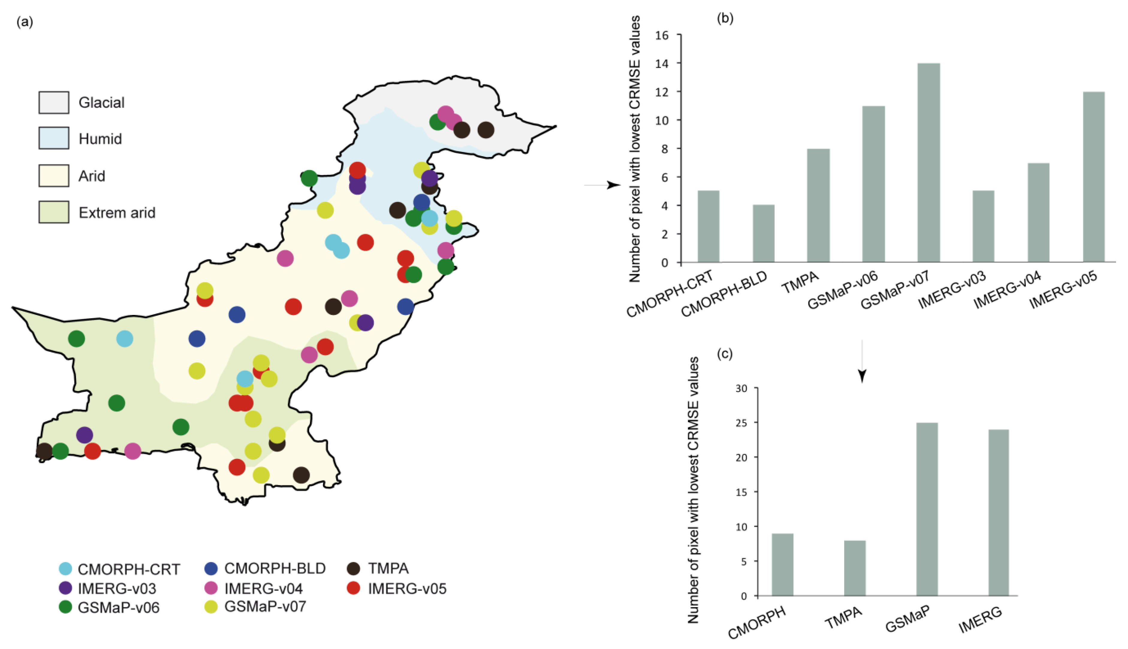
3.6. Benefits of GPM over TRMM Based SPEs

Figure 12 shows the SPEs with the highest performance at the monthly time step in terms of CRMSE. A strong heterogeneity is observed with all SPEs that are represented with at least one pixel over all considered regions except over the glacial region. Therefore, no SPEs consistently outperformed the others. At the regional scale, with 14 and 12 pixels, GSMaP–v07 and IMERG–v05, respectively, are the most represented SPEs (Figure 12b). It highlights the global enhancement from TRMM based SPEs to the lastest GPM based SPEs versions.
More generally, GPM based SPEs (GSMaP and IMERG) are significantly more represented than TRMM based SPEs (CMORPH and TMPA) (Figure 12c). It highlights the GPM benefit on the ongoing SPEs generation. However, for some pixels that are mainly located in the central arid Pakistan region, CMORPH and TMPA still outperformed the GSMaP and IMERG datasets.

4. Discussion

Numerous studies reported on GPM based SPEs accuracy in different regions. However, yet, none study reported on the potential benefit brought by the successive IMERG and GSMaP available versions. Therefore, it should be reminded that this is the first study reporting on IMERG–v05 performance and considering the potential benefit that is brought by IMERG–v05 over its two previously released versions (IMERG–v03, –v04). Regarding GSMaP, this is the first study reporting on both GSMaP–v06 and –v07.
Interestingly, at the regional scale and monthly time step, IMERG–v03 outperformed IMERG–v04, which is in line with previous observations that were made at the daily time step over China [32,33]. This unexpected feature is also observed over the humid and arid regions. However, the very last IMERG–v05 version consists in a real enhancement, as it provides more accurate precipitation estimates than its two previous versions at the regional scale and over both humid and arid regions. Interestingly, the enhancement in precipitation estimates that is brought by the successive IMERG versions (–v03, –v04, –v05) is much marked at the daily than monthly timescale (Figure 7 and Figure 9). All the considered IMERG versions use monthly gauge adjustment (GPCC), so the precipitation estimates at the monthly timescale is strongly dependent on the gauge adjustment. Actually, IMERG similar performance at the monthly timescale means that this component of the algorithms has improved little from IMERG–v03 to –v05 (Figure 7). On the other hand, IMERG estimates at daily timescale are more dependent on other components of the algorithms. Therefore, IMERG precipitation improvement at the daily timescale is a reflection of IMERG algorithms enhancement from IMERG–v03 to –v05 (Figure 10).
Regarding GSMaP datasets, as expected, GSMaP–v07 systematically provides a more realistic precipitation estimate than its previous GSMaP–v06 version at the monthly scale. However, the enhancement is very small, bringing inconsistencies locally. Currently, no studies are available to compare our findings regarding to IMERG–v05 and GSMaP–v07, and therefore other regions should be considered to reinforce the results of the present study.
When comparing the last GPM based SPE versions (IMERG–v05, GSMaP–v07) performance, IMERG–v05 and GSMaP–v07 performed better at the monthly and daily timescale, respectively (Figure 5 and Figure 9). This difference might be the consequence of the gauges adjustment used for IMERG–v05 and GSMaP–v07 processing. Actually, IMERG–v05 relies on a monthly gauge adjustment (GPCC), whereas GSMaP–v07 relies on a daily gauge adjustment (CPC). On a similar way, regarding TRMM based SPEs (CMORPH–BLD and TMPA), CMORPH–BLD (CPC daily gauge adjustment) systematically performed better than TMPA (GPCC monthly gauge adjustment) at the daily timescale. Therefore, the gauges adjustment step appeared to be a considerably influencing factor in SPEs performance.
On a general way, all the SPEs are unsuitable over the glacial region with very low statistical scores at both monthly and daily time steps. This is related to PMW difficulties to retrieve accurate precipitation estimates over the frozen area, which appear to be similar to ice precipitation aloft in the scattering signal in microwave channels on satellites [46,47,48]. Therefore, SPEs algorithms have difficulties in distinguishing between the emission from frozen surfaces and the scattering from ice precipitation aloft. As a result, all of the tested SPEs globally overestimate precipitation over Pakistani glacial region (Figure 8), which is in line with the previous study results focused on TRMM based SPEs [35].
Overall, SPEs relative performance ranking highly varies according to the considered region and the considered pixels. Actually, despite an overall better performance for GPM than TRMM based SPEs, none of the SPEs systematically outperformed the others (Figure 12). In this line, SPEs merging should be considered to take advantages from all available SPEs. Previous studies have already reported on the benefit of such an approach to retrieve the most realistic satellite based precipitation estimates. For example, the blended MSWEP precipitation estimates [8,49] which merge precipitation estimate from (i) different SPEs, (ii) gauges observation and (iii) atmospheric model was tested over the Lake Titicaca basin. In comparison to 11 SPEs, MSWEP provided the most realistic precipitation estimate at the gauge level and the most realistic streamflow and snow–cover simulation if used as a forcing data in the models [50]. In this line, [51] merged TMPA, CMORPH, and PERSIANN datasets to retrieve precipitation estimates over the Tibetan plateau. The merge product was found to outperform MSWEP estimates at both gauges and for streamflow simulation. However, those merged product did not include GPM based SPEs. Therefore according to the present study, future SPE merging attempt should be considered using IMERG and GSMaP datasets as they provide the most accurate precipitation estimates over most regions of the Pakistan.
It is worth mentioning that this study only considers gauge based assessment. Indeed, SPEs potential conclusions may differ when using different indicators than precipitation gauges and especially when comparing SPEs relative performance [50]. Therefore, future study should test GPM based SPEs as forcing data in hydrological modelling to complete the present study. However, such efforts are still complicated, as only four years data are available for IMERG and GSMaP, which compromise models calibration/validation steps.
Finally, the SPEs analysis at the daily time step should be taken with caution as spatial representability between areal (SPE pixel) and point (gauges) measurement may suffer some inconsistency. Indeed, precipitation event detected by the SPE may not be detected by the gauges as it might be raining in other point location of the pixel area [15,35,44]. In this line, a recent study shows that SPEs potential conclusions should be influenced by the reference gauges density used for the assessment [52]. Therefore, similar protocol should be reiterated while using a denser gauges precipitation network to provide robustness results and conclusions on the considered SPEs performance.

5. Conclusions

The present study is a first attempt to highlight the potential benefits that are brought from the successive released versions of GPM based SPEs. IMERG–v03, –v04, –v05 and GSMaP–06, v07 were successively assessed at the daily and monthly times scales over the contrasted geomorphologic and climatic divisions of Pakistan. An inter-comparison between SPE products from GPM with its predecessor TRMM is also included in this study that has increased the merits of this study. Despite the limited coverage and scarcity of the ground reference points, some consistent features emerged from the analysis:
  • SPEs accuracy is region dependent with variable ranking in SPEs performance according to the considered region. All SPEs have presented a strong deficiency over the glacial regions that will remain a major challenge for the future SPEs algorithm development. Additionally, for the same region, the SPEs ranking changed at the very local pixel scale.
  • When considering IMERG datasets, IMERG–v04 should be taken as a well named transitional version between IMERG–v03 and –v05. Indeed, with the exception of the extreme arid region, it has provided globally worst precipitation estimates than its predecessor IMERG–v03. IMERG–v05 fulfilled the expected improvement in precipitation estimates with more realistic precipitation estimates than its predecessor IMERG–v03 and –v04 at both monthly and daily timescale, except over the extreme arid region where IMERG–v04 appeared as a most suitable IMERG version.
  • Considering GSMaP datasets, at the monthly timescale, the two successive versions (–v06, –v07) have performed quite similarly with an overall light enhancement from GSMaP–v06 to –v07 for all the considered regions. A contradiction is observed at the daily timescale at which GSMaP–v06 become more sensitive to precipitation event detection.
  • When comparing IMERG and GSMaP datasets performance, IMERG monthly precipitation estimates are more realistic than GSMaP ones over the arid and extreme arid regions.
  • When considering TRMM based SPEs, CMORPH–BLD highly outperformed CMORPH–CRT. On a general way, CMORPH–BLD outperformed TMPA, except over the extreme arid region and at the monthly timescale.
  • Overall, the transition from TRMM to GPM constitutes a clear enhancement of precipitation estimates over Pakistan with GPM based SPEs provided more realistic monthly precipitation estimates than TRMM based SPEs.
  • No SPE is found to outperform the others promoting the development of SPEs merging approach to improve the precipitation representation over Pakistan.

Author Contributions

F.S., conceived the experiments and F.S. and Y.H. analysed the data. M.-P.B., Y.H., B.M.H., H.M.-C., G.A., R.U. provided reviews and suggestions. F.S. and Y.H. wrote the paper.

Funding

This research received no external funding.

Acknowledgments

This work is part of a postdoctoral fellowship funded by the CNES (Centre National d’Etudes Spatiales, France). The authors are grateful to SPE datasets providers and to the Pakistan Meteorological Department (PMD) for the in situ precipitation observations.

Conflicts of Interest

The authors declare no conflict of interest.

References

  1. TRMM and Other Data Precipitation Data Set Documentation. Available online: https://www.researchgate.net/profile/George_Huffman/publication/228892338_TRMM_and_Other_Data_Precipitation_Data_Set_Documentation/links/575f0bde08ae9a9c955fac32/TRMM-and-Other-Data-Precipitation-Data-Set-Documentation.pdf (accessed on 13 August 2018).
  2. Joyce, R.J.; Janowiak, J.E.; Arkin, P.A.; Xie, P. CMORPH: A Method that Produces Global Precipitation Estimates from Passive Microwave and Infrared Data at High Spatial and Temporal Resolution. J. Hydrometeorol. 2004, 5, 487–803. [Google Scholar] [CrossRef]
  3. Sorooshian, S.; Hsu, K.-L.; Gao, X.; Gupta, H.V.; Imam, B.; Braithwaite, D. Evaluation of PERSIANN System Satellite–Based Estimates of Tropical Rainfall. Bull. Am. Meteorol. Soc. 2000, 81, 2035–2046. [Google Scholar] [CrossRef] [Green Version]
  4. GSMaP. User’s Guide for Global Satellite Mapping of Precipitation Microwave-IR Combined Product (GSMaP_MVK), Version 5. Available online: http://sharaku.eorc.jaxa.jp/GSMaP/document/DataFormatDescription_MVK&RNL_v6.5133A.pdf (accessed on 13 August 2018).
  5. Maggioni, V.; Meyers, P.C.; Robinson, M.D. A Review of Merged High-Resolution Satellite Precipitation Product Accuracy during the Tropical Rainfall Measuring Mission (TRMM) Era. J. Hydrometeorol. 2016, 17, 1101–1117. [Google Scholar] [CrossRef]
  6. Sun, Q.; Miao, C.; Duan, Q.; Ashouri, H.; Sorooshian, S.; Hsu, K.-L. A review of global precipitation datasets: data sources, estimation, and intercomparisons. Rev. Geograp. 2018, 56, 79–107. [Google Scholar] [CrossRef]
  7. Ashouri, H.; Hsu, K.L.; Sorooshian, S.; Braithwaite, D.K.; Knapp, K.R.; Cecil, L.D.; Nelson, B.R.; Prat, O.P. PERSIANN-CDR: Daily precipitation climate data record from multisatellite observations for hydrological and climate studies. Bull. Am. Meteorol. Soc. 2015, 96, 69–83. [Google Scholar] [CrossRef]
  8. Beck, H.E.; Vergopolan, N.; Pan, M.; Levizzani, V.; van Dijk, A.I.J.M.; Weedon, G.; Brocca, L.; Pappenberger, F.; Huffman, G.J.; Wood, E.F. Global-scale evaluation of 23 precipitation datasets using gauge observations and hydrological modeling. Hydrol. Earth Syst. Sci. Discuss. 2017. [Google Scholar] [CrossRef]
  9. Funk, C.; Peterson, P.; Landsfeld, M.; Pedreros, D.; Verdin, J.; Shukla, S.; Husak, G.; Rowland, J.; Harrison, L.; Hoell, A.; et al. The climate hazards infrared precipitation with stations—A new environmental record for monitoring extremes. Sci. Data 2015. [CrossRef] [PubMed]
  10. Agutu, N.O.; Awange, J.L.; Zerihun, A.; Ndehedehe, C.E.; Kuhn, M.; Fukuda, Y. Assessing multi-satellite remote sensing, reanalysis, and land surface models’ products in characterizing agricultural drought in East Africa. Remote Sens. Environ. 2017, 194, 287–302. [Google Scholar] [CrossRef]
  11. Bayissa, Y.; Tadesse, T.; Demisse, G.; Shiferaw, A. Evaluation of satellite-based rainfall estimates and application to monitor meteorological drought for the Upper Blue Nile Basin, Ethiopia. Remote Sens. 2017, 9, 669. [Google Scholar] [CrossRef]
  12. Satgé, F.; Espinoza, R.; Zolá, R.; Roig, H.; Timouk, F.; Molina, J.; Garnier, J.; Calmant, S.; Seyler, F.; Bonnet, M.-P. Role of Climate Variability and Human Activity on Poopó Lake Droughts between 1990 and 2015 Assessed Using Remote Sensing Data. Remote Sens. 2017, 9, 218. [Google Scholar] [CrossRef]
  13. Casse, C.; Gosset, M. Analysis of hydrological changes and flood increase in Niamey based on the PERSIANN-CDR satellite rainfall estimate and hydrological simulations over the 1983–2013 period. IAHS-AISH Proc. Rep. 2015, 370, 117–123. [Google Scholar] [CrossRef] [Green Version]
  14. Integrated Multi-satellitE Retrievals for GPM (IMERG) Technical Documentation. Available online: https://docserver.gesdisc.eosdis.nasa.gov/public/project/GPM/IMERG_doc.05.pdf (accessed on 13 August 2018).
  15. Satgé, F.; Xavier, A.; Zolá, R.; Hussain, Y.; Timouk, F.; Garnier, J.; Bonnet, M.-P. Comparative Assessments of the Latest GPM Mission’s Spatially Enhanced Satellite Rainfall Products over the Main Bolivian Watersheds. Remote Sens. 2017, 9, 369. [Google Scholar] [CrossRef]
  16. Liu, Z. Comparison of Integrated Multisatellite Retrievals for GPM (IMERG) and TRMM Multisatellite Precipitation Analysis (TMPA) Monthly Precipitation Products: Initial Results. J. Hydrometeorol. 2016, 17, 777–790. [Google Scholar] [CrossRef]
  17. Prakash, S.; Mitra, A.K.; AghaKouchak, A.; Liu, Z.; Norouzi, H.; Pai, D.S. A preliminary assessment of GPM-based multi-satellite precipitation estimates over a monsoon dominated region. J. Hydrol. 2016, 556, 865–876. [Google Scholar] [CrossRef]
  18. Tang, G.; Ma, Y.; Long, D.; Zhong, L.; Hong, Y. Evaluation of GPM Day-1 IMERG and TMPA Version-7 legacy products over Mainland China at multiple spatiotemporal scales. J. Hydrol. 2016, 533, 152–167. [Google Scholar] [CrossRef]
  19. Chen, F.; Li, X. Evaluation of IMERG and TRMM 3B43 Monthly Precipitation Products over Mainland China. Remote Sens. 2016, 8, 472. [Google Scholar] [CrossRef]
  20. Wang, Z.; Zhong, R.; Lai, C.; Chen, J. Evaluation of the GPM IMERG satellite-based precipitation products and the hydrological utility. Atmos. Res. 2017, 196, 151–163. [Google Scholar] [CrossRef]
  21. Kim, K.; Park, J.; Baik, J.; Choi, M. Evaluation of topographical and seasonal feature using GPM IMERG and TRMM 3B42 over Far-East Asia. Atmos. Res. 2017, 187, 95–105. [Google Scholar] [CrossRef]
  22. Tan, M.L.; Duan, Z. Assessment of GPM and TRMM precipitation products over Singapore. Remote Sens. 2017, 9, 720. [Google Scholar] [CrossRef]
  23. Sharifi, E.; Steinacker, R.; Saghafian, B. Assessment of GPM-IMERG and Other Precipitation Products against Gauge Data under Different Topographic and Climatic Conditions in Iran: Preliminary Results. Remote Sens. 2016, 8, 135. [Google Scholar] [CrossRef]
  24. Oliveira, R.; Maggioni, V.; Vila, D.; Morales, C. Characteristics and Diurnal Cycle of GPM Rainfall Estimates over the Central Amazon Region. Remote Sens. 2016, 8, 544. [Google Scholar] [CrossRef]
  25. Mahmoud, M.T.; Al-Zahrani, M.A.; Sharif, H.O. Assessment of Global Precipitation Measurement Satellite Products over Saudi Arabia. J. Hydrol. 2018, 559, 1–12. [Google Scholar] [CrossRef]
  26. Sharifi, E.; Steinacker, R.; Saghafian, B. Multi time-scale evaluation of high-resolution satellite-based precipitation products over northeast of Austria. Atmos. Res. 2018, 206, 46–63. [Google Scholar] [CrossRef]
  27. Sungmin, O.; Foelsche, U.; Kirchengast, G.; Fuchsberger, J.; Tan, J.; Petersen, W.A. Evaluation of GPM IMERG Early, Late, and Final rainfall estimates using WegenerNet gauge data in southeastern Austria. Hydrol. Earth Syst. Sci. 2017, 21, 6559–6572. [Google Scholar] [CrossRef] [Green Version]
  28. Tan, M.L.; Santo, H. Comparison of GPM IMERG, TMPA 3B42 and PERSIANN-CDR satellite precipitation products over Malaysia. Atmos. Res. 2018, 202, 63–76. [Google Scholar] [CrossRef]
  29. Chiaravalloti, F.; Brocca, L.; Procopio, A.; Massari, C.; Gabriele, S. Assessment of GPM and SM2RAIN-ASCAT rainfall products over complex terrain in southern Italy. Atmos. Res. 2018, 206, 64–74. [Google Scholar] [CrossRef]
  30. Anjum, M.N.; Ding, Y.; Shangguan, D.; Ahmad, I.; Ijaz, M.W.; Farid, H.U.; Yagoub, Y.E.; Zaman, M.; Adnan, M. Performance evaluation of latest integrated multi-satellite retrievals for Global Precipitation Measurement (IMERG) over the northern highlands of Pakistan. Atmos. Res. 2018, 205, 134–146. [Google Scholar] [CrossRef]
  31. Muhammad, W.; Yang, H.; Lei, H.; Muhammad, A.; Yang, D. Improving the regional applicability of satellite precipitation products by ensemble algorithm. Remote Sens. 2018, 10, 577. [Google Scholar] [CrossRef]
  32. Wei, G.; Lü, H.; Crow, W.T.; Zhu, Y.; Wang, J.; Su, J. Evaluation of satellite-based precipitation products from IMERG V04A and V03D, CMORPH and TMPA with gauged rainfall in three climatologic zones in China. Remote Sens. 2018, 10, 30. [Google Scholar] [CrossRef]
  33. Zhao, H.; Yang, S.; You, S.; Huang, Y.; Wang, Q.; Zhou, Q. Comprehensive evaluation of two successive V3 and V4 IMERG final run precipitation products over Mainland China. Remote Sens. 2018, 10, 34. [Google Scholar] [CrossRef]
  34. Adnan, S.; Ullah, K.; Gao, S.; Khosa, A.H.; Wang, Z. Shifting of agro-climatic zones, their drought vulnerability, and precipitation and temperature trends in Pakistan. Int. J. Climatol. 2017, 37, 529–543. [Google Scholar] [CrossRef]
  35. Hussain, Y.; Satgé, F.; Hussain, M.B.; Martinez-Caravajal, H.; Bonnet, M.-P.; Cardenas-Soto, M.; Llacer Roig, H.; Akhter, G. Performance of CMORPH, TMPA and PERSIANN rainfall datasets over plain, mountainous and glacial regions of Pakistan. Theor. Appl. Climatol. 2017. [Google Scholar] [CrossRef]
  36. Huffman, G.; Bolvin, D.; Braithwaite, D.; Hsu, K.; Joyce, R. Algorithm Theoretical Basis Document (ATBD) NASA Global Precipitation Measurement (GPM) Integrated Multi-satellitE Retrievals for GPM (IMERG). Available online: https://pmm.nasa.gov/sites/default/files/document_files/IMERG_ATBD_V5.2_0.pdf (accessed on 13 August 2018).
  37. Shige, S.; Yamamoto, T.; Tsukiyama, T.; Kida, S.; Ashiwake, H.; Kubota, T.; Seto, S.; Aonashi, K.; Okamoto, K. The GSMaP precipitation retrieval algorithm for microwave sounders part I: Over-ocean algorithm. IEEE Trans. Geosci. Remote Sens. 2009, 47, 3084–3097. [Google Scholar] [CrossRef]
  38. Ushio, T.; Sasashige, K.; Kubota, T.; Shige, S.; Okamoto, K.; Aonashi, K.; Inoue, T.; Takahashi, N.; Iguchi, T.; Kachi, M.; et al. A Kalman Filter Approach to the Global Satellite Mapping of Precipitation (GSMaP) from Combined Passive Microwave and Infrared Radiometric Data. J. Meteorol. Soc. Jpn. 2009, 87A, 137–151. [Google Scholar] [CrossRef]
  39. Bias-Corrected CMORPH: A 13-Year Analysis of High-Resolution Global Precipitation Objective. Available online: https://meetingorganizer.copernicus.org/EGU2011/EGU2011-1809.pdf (accessed on 13 August 2018).
  40. Xie, P.; Xiong, A.Y. A conceptual model for constructing high-resolution gauge-satellite merged precipitation analyses. J. Geophys. Res. Atmos. 2011, 116, 1–14. [Google Scholar] [CrossRef]
  41. World Meteorological Organization Guide to Hydrological Practices: Data Acquisition and Processing, Analysis, Forecasting And Other Applications; 1994. Available online: http://www.innovativehydrology.com/WMO-No.168-1994.pdf (accessed on 13 August 2018).
  42. Taylor, K.E. Summarizing multiple aspects of model performance in a single diagram. J. Geophys. Res. 2001, 106, 7183–7192. [Google Scholar] [CrossRef] [Green Version]
  43. Ochoa, A.; Pineda, L.; Crespo, P.; Willems, P. Evaluation of TRMM 3B42 precipitation estimates and WRF retrospective precipitation simulation over the Pacific–Andean region of Ecuador and Peru. Hydrol. Earth Syst. Sci. 2014, 18, 3179–3193. [Google Scholar] [CrossRef] [Green Version]
  44. Satgé, F.; Bonnet, M.-P.; Gosset, M.; Molina, J.; Hernan Yuque Lima, W.; Pillco Zolá, R.; Timouk, F.; Garnier, J. Assessment of satellite rainfall products over the Andean plateau. Atmos. Res. 2016, 167, 1–14. [Google Scholar] [CrossRef]
  45. Roebber, P.J. Visualizing Multiple Measures of Forecast Quality. Weather Forecast. 2009, 24, 601–608. [Google Scholar] [CrossRef]
  46. Mourre, L.; Condom, T.; Junquas, C.; Lebel, T.; Sicart, J.E.; Figueroa, R.; Cochachin, A. Spatio-temporal assessment of WRF, TRMM and in situ precipitation data in a tropical mountain environment (Cordillera Blanca, Peru). Hydrol. Earth Syst. Sci. 2016, 20, 125–141. [Google Scholar] [CrossRef] [Green Version]
  47. Levizzani, V.; Amorati, R.; Meneguzzo, F. A Review of Satellite-Based Rainfall Estimation Methods. Available online: http://satmet.isac.cnr.it/papers/MUSIC-Rep-Sat-Precip-6.1.pdf (accessed on 13 August 2018).
  48. Ferraro, R.R.; Smith, E.A.; Berg, W.; Huffman, G.J. A Screening Methodology for Passive Microwave Precipitation Retrieval Algorithms. J. Atmos. Sci. 1998, 55, 1583–1600. [Google Scholar] [CrossRef]
  49. Beck, H.E.; van Dijk, A.I.J.M.; Levizzani, V.; Schellekens, J.; Miralles, D.G.; Martens, B.; de Roo, A. MSWEP: 3-hourly 0.25° global gridded precipitation (1979–2015) by merging gauge, satellite, and reanalysis data. Hydrol. Earth Syst. Sci. Discuss. 2016, 21, 589–615. [Google Scholar] [CrossRef]
  50. Satgé, F.; Ruelland, D.; Bonnet, M.-P.; Molina, J.; Pillco, R. Consistency of satellite precipitation estimates in space and over time compared with gauge observations and snow-hydrological modelling in the lake Titicaca region. Hydrol. Earth Syst. Sci. 2018. submitted. [Google Scholar]
  51. Ma, Y.; Yang, Y.; Han, Z.; Tang, G.; Maguire, L.; Chu, Z.; Hong, Y. Comprehensive evaluation of Ensemble Multi-Satellite Precipitation Dataset using the Dynamic Bayesian Model Averaging scheme over the Tibetan Plateau. J. Hydrol. 2017, 556, 634–644. [Google Scholar] [CrossRef]
  52. Tang, G.; Behrangi, A.; Long, D.; Li, C.; Hong, Y. Accounting for spatiotemporal errors of gauges: A critical step to evaluate gridded precipitation products. J. Hydrol. 2018, 559, 294–306. [Google Scholar] [CrossRef]
Figure 1. Study area with the location of precipitation gauges used as references. (a) Pakistan elevation derived from the Shuttle Radar Topography Model (SRTM). (b) Location of the four considered climatic zones.
Remotesensing 10 01373 g001
Figure 2. Annual precipitation maps for 2015 retrieved from all Satellite Precipitation Estimates (SPEs) at their original grid size. For each SPEs, only the pixels with more than 80% available daily data were considered.
Remotesensing 10 01373 g002
Figure 3. Gauges network used to produce (a) CPC (0.5°) and (b) GPCC (1°) gauges based precipitation grid for the year 2015 with gauges network used as reference data in the present study.
Remotesensing 10 01373 g003
Figure 4. Available precipitations estimates from all SPEs and gauges for the 2015 year at (a) daily and (b) monthly time steps.
Remotesensing 10 01373 g004
Figure 5. SPEs monthly performance for all the considered regions expressed in form of Taylor diagram. The reference black dot represents the perfect statistical scores (CC = 1, STD = 1, CRMSE = 0). Centered Root Mean Square Error (CRMSE) is represented by curved solid grey lines.
Remotesensing 10 01373 g005
Figure 6. %B for all considered SPEs and all the considered regions.
Remotesensing 10 01373 g006
Figure 7. SPEs performance at the gauges point measurement expressed in form of CRMSE.
Remotesensing 10 01373 g007
Figure 8. SPEs performance at the gauges point measurement expressed in form of %B.
Remotesensing 10 01373 g008
Figure 9. SPEs daily performance expressed in form of performance diagram. Curved lines and straight lines represent the CSI and Bias values, respectively. The reference black dot represents the perfect statistical scores (POD = 1, SR = 1, Bias = 1 and CSI = 1).
Remotesensing 10 01373 g009
Figure 10. SPEs performance at the daily time step expressed in form of Heidke Skill Score (HSS) index.
Remotesensing 10 01373 g010
Figure 11. Improvement on monthly precipitation estimates from successive Global Precipitation Measurement (GPM) based SPEs: best SPEs version from successive Global Satellite Mapping of Precipitation (GSMaP) (a) and Integrated Multi–Satellite Retrievals for GPM (IMERG) (b) versions based on CRMSE values; absolute difference of CRMSE value between the most and least accurate GSMaP versions (c) and IMERG versions (d).
Remotesensing 10 01373 g011
Figure 12. SPEs with the highest performance among all considered SPEs in term of CRMSE. (a) Spatial distribution of SPEs ranking in term of CRMSE, (b) numbers of pixels in which the considered SPEs outperformed the others, and (c) same as (b) but aggregated to the SPEs group.
Remotesensing 10 01373 g012
Table 1. Main features of the considered regions. Annual average precipitations are derived from Tropical Rainfall Measuring Mission Multisatellite Precipitation Analysis (TMPA) over the 1998–2017 period and average elevation are derived from the Shuttle Radar Topography Model (SRTM).
RegionPakistanHumidGlacialAridExtreme Arid
Surface area (km2)878.400115.81082.070396.320286.511
Average elevation (m)104412864158633444
Annual average precipitation (mm)338852348322133
Number of stations882683222
Table 2. Contingency table used to define daily categorical scores for the verification of SPEs against gauge data.
Gauges (Pref)
PrecipitationNo precipitation
SPEPrecipitationab
No Precipitationcd

