Colour Classification of 1486 Lakes across a Wide Range of Optical Water Types


1
Environmental Research Institute, The University of Waikato, Private Bag 3105, Hamilton 3216, New Zealand
2
Institute for Environmental Studies (IVM), Water & Climate Risk, VU University Amsterdam, De Boelelaan 1087, 1081HV Amsterdam, The Netherlands
*
Author to whom correspondence should be addressed.
Remote Sens. 2018, 10(8), 1273; https://doi.org/10.3390/rs10081273
Submission received: 1 July 2018
/
Revised: 7 August 2018
/
Accepted: 9 August 2018
/
Published: 13 August 2018
(This article belongs to the Special Issue Remote Sensing of Inland Waters and Their Catchments)
Abstract
:Remote sensing by satellite-borne sensors presents a significant opportunity to enhance the spatio-temporal coverage of environmental monitoring programmes for lakes, but the estimation of classic water quality attributes from inland water bodies has not reached operational status due to the difficulty of discerning the spectral signatures of optically active water constituents. Determination of water colour, as perceived by the human eye, does not require knowledge of inherent optical properties and therefore represents a generally applicable remotely-sensed water quality attribute. In this paper, we implemented a recent algorithm for the retrieval of colour parameters (hue angle, dominant wavelength) and derived a new correction for colour purity to account for the spectral bandpass of the Landsat 8 Operational Land Imager (OLI). We used this algorithm to calculate water colour on almost 45,000 observations over four years from 1486 lakes from a diverse range of optical water types in New Zealand. We show that the most prevalent lake colours are yellow-orange and blue, respectively, while green observations are comparatively rare. About 40% of the study lakes show transitions between colours at a range of time scales, including seasonal. A preliminary exploratory analysis suggests that both geo-physical and anthropogenic factors, such as catchment land use, provide environmental control of lake colour and are promising avenues for future analysis.
1. Introduction
The colour of water as perceived by a human observer is intuitively associated with its suitability for consumption, quality of food collection, fitness for recreation, and aesthetic value, making it arguably one of the oldest water-quality attributes [1,2,3]. Water colour is integral to the concept of optical water quality, which may be defined as “the extent to which the suitability of water for its functional role in the biosphere or the human environment is determined by its optical properties” [4].
Perceived colour is the physiological sensation originating from the sensitivity of the human eye to light in the spectral range of the primary colours red, blue, and green e.g., [5]. The standard colorimetric system of the Commission Internationale de l’Éclairage (CIE) [6] defines colour mathematically by weighting the light spectrum with the three mixing curves, or chromaticity curves, specifying the respective sensitivity of the human eye to the primary colours. In the case of water, a medium that is not self-luminous, the light perceived by an observer is sunlight scattered back from within the water mass. This upwelling light is of a different colour than the incident solar radiation due to wavelength-dependent absorption and scattering of light by water and its constituents [7].
The absorption spectrum of pure water has a minimum in the blue to green range of the visible spectrum of light and it is much higher at red and near-infrared wavelengths. In addition, scattering by water molecules is stronger at shorter wavelengths causing more of the incoming blue light to be directed back at the observer [8]. Therefore, water that is characterised by the absence of absorbing and scattering constituents is blue and is popularly perceived as ‘clean’—an often justifiable judgement. The main constituents that give water a colour other than blue are phytoplankton pigments, such as chlorophyll a (chl a), suspended particulate matter (SPM) and coloured dissolved organic matter (CDOM) [9,10]. The perceived water colours in hues of green, yellow, and brown are thus generally related to predominance of optical effects by phytoplankton, SPM, and CDOM, respectively (Figure 1). In optically simple cases, i.e., when one of these constituents dominates the absorption and scattering of light, water colour is related to the concentration of the dominant constituent and its inherent optical properties (IOPs), but in complex mixtures, the spectral signatures are potentially not uniquely separable [11,12].
The derivation of concentrations of chl a, SPM and CDOM in inland waters from multispectral observations such as those recorded by earth-orbiting satellites is an active area of research [7,14,15,16]. However, the wide range of concentrations of chl a, SPM, CDOM, and their independent variability hinder efforts to develop general algorithms for the retrieval of these constituents that work across a wide range of lake systems [17]. Therefore, studies reporting retrieval of inland water quality across several lakes are tailored to lakes with comparable optical properties [18,19,20].
Algorithms have been developed for the retrieval of colour information from ocean-colour sensors and a suite of medium resolution sensors [21,22]. This colour information is based only on the remote sensing reflectance and can be retrieved accurately and consistently from sensors with four or more spectral bands in the visual domain. Since colour estimation does not rely on knowledge of IOPs of optically active constituents in the water, it provides an objective water quality attribute across any optical water type.
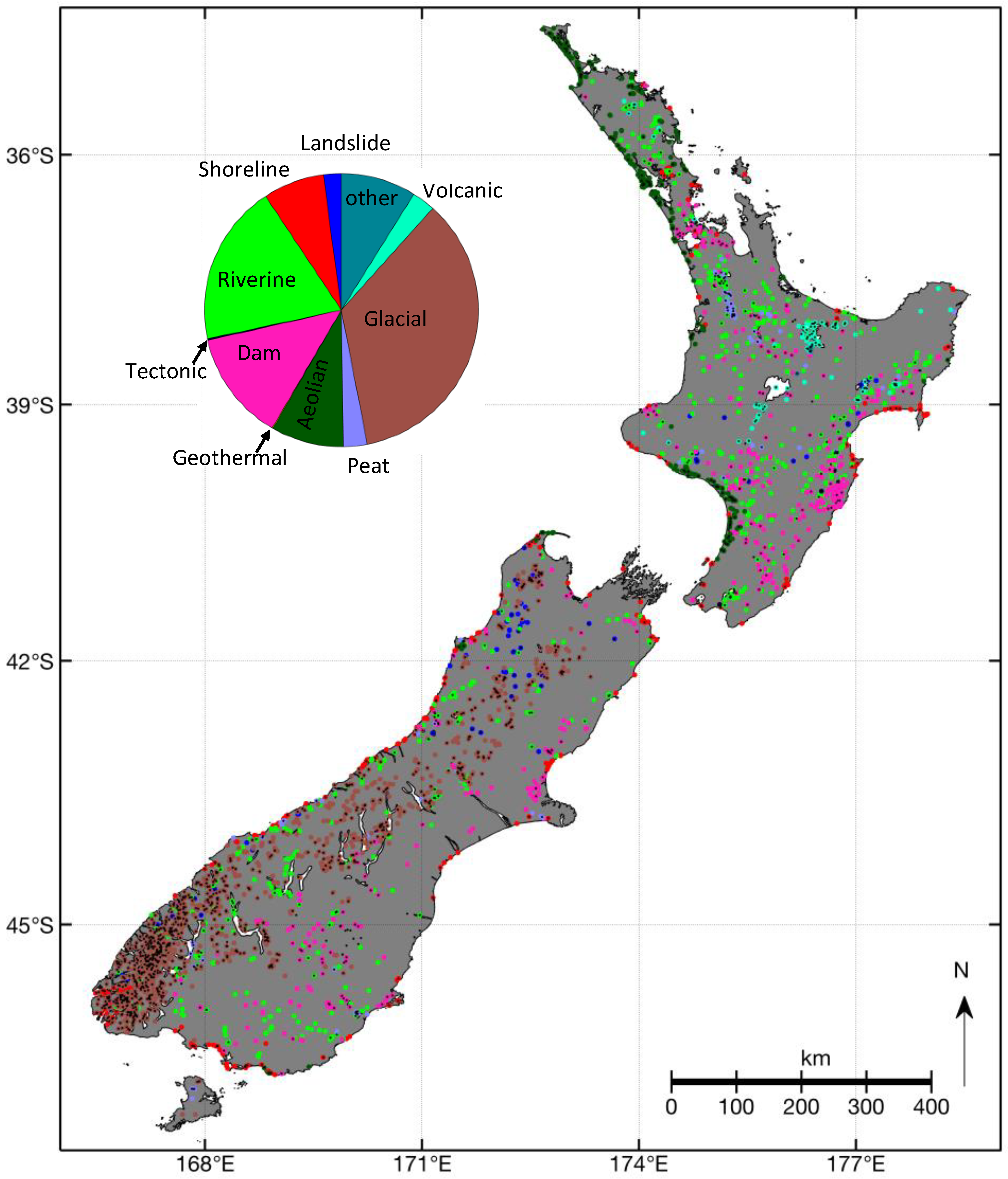
The goal of this study is to establish a methodology for satellite-based water colour assessment at the national scale of New Zealand and to demonstrate its usefulness by relating it to geomorphology and primary drivers of water quality. In New Zealand, versatile geology and climatic gradients have produced a wide range of lake types [23], which, in combination with strong gradients of anthropogenic pressures, produce a comprehensive range of optical water types [24,25,26]. The Freshwater Ecosystems of New Zealand geodatabase (FENZ) [27,28] identifies 3820 lakes with a surface area greater than one hectare (Figure 2), and obviously, traditional monitoring of water quality of a large number of lakes represents considerable logistical and financial challenges. Data on water quality is available for less than 2% of New Zealand’s lakes [29,30,31].
Remote sensing has the potential to address this knowledge gap by providing current baseline information and historic data for any lake large enough to be resolved by the footprint of satellite sensors. Here, we derive water colour using the hue angle method of Woerd and Wernand [22] from over 1400 lakes across New Zealand using atmospherically corrected reflectance derived from Landsat 8 OLI images that were captured between April 2013 and February 2018. We demonstrate the monitoring capability of this product at the national scale by relating it to expected correlates of water quality, such as lake depth, elevation, and land use.
2. Materials and Methods
2.1. Study Area
The study area includes the entire land mass of New Zealand (268,021 km2) comprised of two major islands that are located in the southern hemisphere between 34.4°S–46.7°S, centred on approximately 173°E (Figure 2). This study considers 3820 freshwater bodies larger than 10,000 m2 (one hectare) as delineated and classified as lakes in the Freshwater Ecosystems of New Zealand geodatabase [27,28]. These water bodies were originally derived from the NZMS 260 1:50,000 topographic map series administered by Land Information New Zealand and include ephemeral flooded areas, wetlands, stormwater retention ponds, and other water bodies, which may not strictly fit definitions of lakes. We use these 3820 “lakes” as a starting set and derived the central point of each lake using the Quantum GIS (QGIS) plugin “real centroid”, which forced the centroid to be inside the lake outline (Figure 3). Subsequently, each centroid was expanded to a circle area of interest (AOI) of 45 m radius and the AOI’s placement was inspected visually against aerial photos [32] to confirm or adjust its location over a central region of the lake away from islands or obvious shallow regions. 2334 lakes were excluded from the analysis, because the AOI could not be placed in openwater or the lakes were considered to be optically shallow, leaving a set of 1486 lakes.
2.2. Satellite Imagery Acquisition and Processing
We chose Landsat 8 Operational Land Imager (OLI) data, because the 30-m pixel resolution allows for the observation of lakes down to about 1 ha size. Furthermore, the Landsat series of satellites provides the longest continuous time series of earth observations from space, allowing for retrospective analysis of colour trends in future work. The OLI collects data in eight bands at 30 m resolution and one panchromatic band at 15 m resolution [33]. 1521 OLI images that were captured along paths 71 to 75 and rows 84 through 93, between 12 April 2013, and 12 February 2018 from the Tier 1 collection were downloaded from the USGS Earth Resources Observation and Science (EROS) Center Science Processing Architecture (ESPA) on-demand interface.
The Tier 1 collection provides surface reflectance, ρ (sr−1), at each band. ρ is a level-2 product resulting from atmospheric correction with the Landsat Surface Reflectance Code (LaSRC), which uses the coastal aerosol band and auxiliary climate data from MODIS with a radiative transfer model designed for Landsat 8 [34,35]. We approximate surface remote sensing reflectance (R, sr−1) as ρ/π and note that this introduces some error as ρ includes contributions from specular reflectance at the water surface (glint) [36] and from whitecaps [37]. However, as these contributions are spectrally flat, they have an effect on purity, but not on dominant wavelength (see further down for definition of these terms). Limitations of this approximation are presented in the Discussion. The Tier 1 collection also includes quality attributes for each pixel determined using the CFMask algorithm, which we used to exclude pixels with values indicating cloud, adjacent shadow, cloud shadow, and cirrus [34,38,39]. An additional NDWI [40] mask was applied to reduce the chance for data from optically shallow water. Lake reflectance of each band was calculated by averaging R(λ) from 9 to 16 pixels, which intersected the AOI of each lake. Pixels for which reflectance in any of the bands were negative or greater than one were excluded from the averaging. This procedure generated a file with 44,947 observations for 1486 New Zealand lakes between 2013 and 2018.
The number of good observations, i.e., cloud-free with reflectance values between zero and one, was recorded for each lake. In cases where there are duplicate observations from the zone of row-overlap, only the data from the earlier scene was retained. We define the expected number of observations per year by Landsat OLI for every lake by dividing the number of good observations by 4.08, which is the number of years in our data set.
2.3. Calculation of Chromaticity
Chromaticity analysis describes the colour of an object as perceived by the human eye using three colour primaries X, Y, and Z, also known as tristimulus values [12]. The tristimulus values X, Y, and Z are integrals of the weighted upwelling reflectance spectrum R(λ) within the region to which the human eye is sensitive (390–740 nm). The weighting functions , and are the colour mixture values, which describe the wavelength dependence of human vision for red, green, and blue light, respectively [6,12]:
The chromaticity coordinates x, y and z are normalisations of the individual tristimulus values, as follows:
with x + y + z = 1.
Satellite remote sensing data from current satellite-borne sensors do not have full spectral coverage, but provide remote sensing reflectance in a limited number of bands of 10 nm wavelength or wider. Landsat 8 OLI has four bands in the visible part of the spectrum that are centred at 443 nm (narrow blue, coastal/aerosol), 482 nm (blue), 562 nm (green), and 655 nm (red) [41,42], and therefore, the estimation of the true colour of upwelling light requires assumptions about the full spectral distribution of remote sensing reflectance. Early chromaticity mapping used radiances from the multispectral scanner carried on Landsat missions 1 to 5 in spectral bands of 100 nm width in the green, red, and near infrared regions of the spectrum, and these radiances were assumed to be analogous to the tristimulus values X, Y, and Z [12,43,44].
Van der Woerd and Wernand [21,22] describe that in first approximation the tristimulus values can be reconstructed based on a linear weighted sum of the bands R, in this case, the four bands of OLI
Chromaticity coordinates are then calculated from the X, Y, and Z using Equations (4)–(6); the perceived colour of a given reflectance spectrum is defined by any pair of chromaticity coordinates and can be plotted in a chromaticity diagram, e.g., x and y, as shown in Figure 1. The horseshoe-shaped envelope (locus) is constructed from the x and y values calculated from monochromatic light at each wavelength and therefore the space enclosed in it encompass all possible chromaticity values. The centre of the chromaticity diagram is the “white point” at which x = y = z = ⅓. Any pair of x, y coordinates of an upwelling radiance spectrum can be identified by the hue angle (α), which is the angle of the line drawn from the white point to the x, y coordinate and the x-axis of the plot in anticlockwise direction. We calculate α using the four quadrant arctangent function atan2 in Matlab (Equation (7) in [22]):
α = arctan(y − 1/3, x − 1/3) modulus 2π.
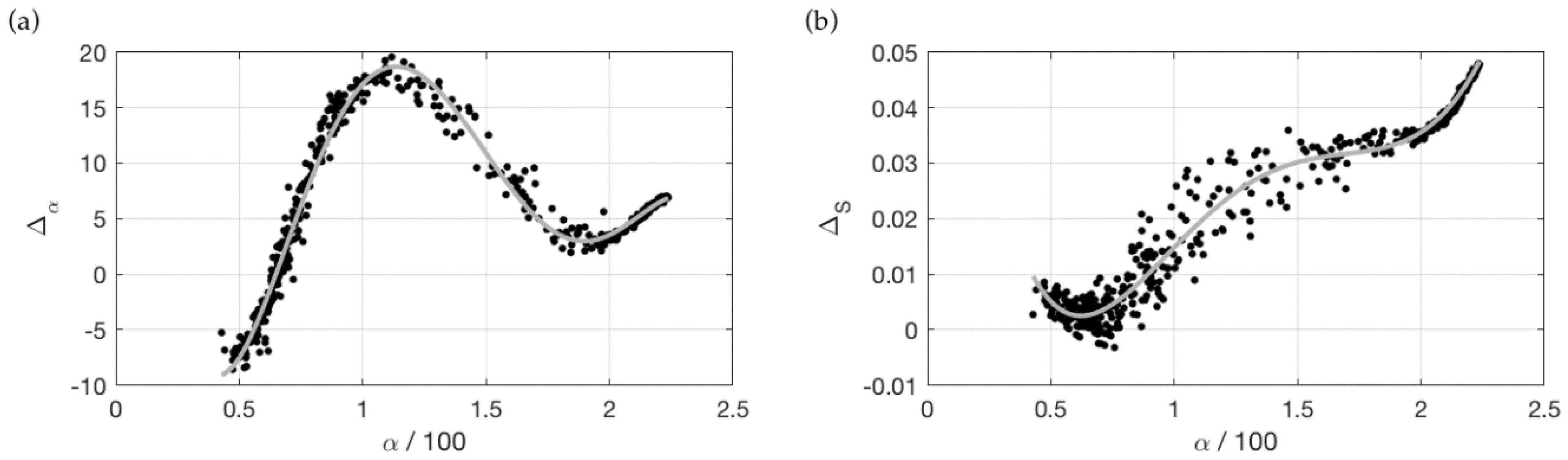
As described in Van der Woerd and Wernand [22], the spectral bandpass of OLI causes an offset between −5 and +20 degrees relative to the hyperspectral hue angle. The offset is not completely random, and as a first approximation, the correction (Δα) can be described by a fifth order polynomial, which is indicated by the grey line in Figure 4a. If a is the calculated hue angle divided by 100, Δα can be approximated (for OLI) by:
Δα = −52.16a5 + 373.81a4 − 981.83a3 + 1134.19a2 − 533.61a + 76.72
Δα is based on calculations using semi-empirical model simulations published by the International Ocean Colour Coordinating Group [9]. The above-water R(λ) is simulated using Hydrolight [45] and a set of inherent optical properties derived from field measurements, representing a wide range of compositions that occur in natural waters. Details on this data set can be found in [9] and the IOCCG website [46]. The 500 synthetic R spectra are provided every 10 nm between 400–800 nm. In this paper, we refer to the “hyperspectral” colour when these spectra are interpolated on a 1-nm grid and α is calculated based on Equations (1)–(6). The observations by OLI are simulated by folding the 1-nm spectra with the detector efficiency for each band, as described by the spectral response function of the OLI on Landsat 8 [47].
The distance (S) of a hyperspectral colour on the chromaticity diagram from the white point is calculated by:
We extend the work of van der Woerd and Wernand [22] by calculating ΔS, a correction for the spectral bandpass of OLI analogous to Δα, by calculating S from x, y pairs derived for the hyperspectral and 4-band OLI case, respectively. With increasing distance from the white point, the colour becomes more intense, until it reaches the locus, the place in the chromaticity diagram for a monochromatic reflection at a specific wavelength. This wavelength is called the dominant wavelength (λd, nm) and the contribution of the dominant wavelength to an observed optical spectrum is termed purity (S*), defined as the ratio of S to the distance between the white point and the spectral locus of the dominant wavelength [12]. We report lake colour in terms of λd instead of α, because it provides an intuitive and illustrative amplification of the observed colour that is useful for plotting and interpretation purposes. λd is derived geometrically from α + Δα by determining the wavelength at the point of intersection with the locus.
To investigate the lake colour characteristics with respect to landuse, we calculated the percentage of land cover of high-producing exotic grassland (P) in each lake’s catchment from the New Zealand Land Cover Database Version 4.1 [48]. This percentage was transformed using the logistic function (log (P/(100-P)) where log is the natural logarithm. Moreover, each lake was assigned to one of eight elevation-depth classes based on the elevation of the lake surface and the maximum depth as given in [29]. The eight classes divide lowland and highland lakes (below and above 300 m above sea level, respectively) and four depth ranges (0–5 m, 5–15 m, 15–50 m, >50 m), respectively.
3. Results
3.1. Observation Frequency of New Zealand Lakes
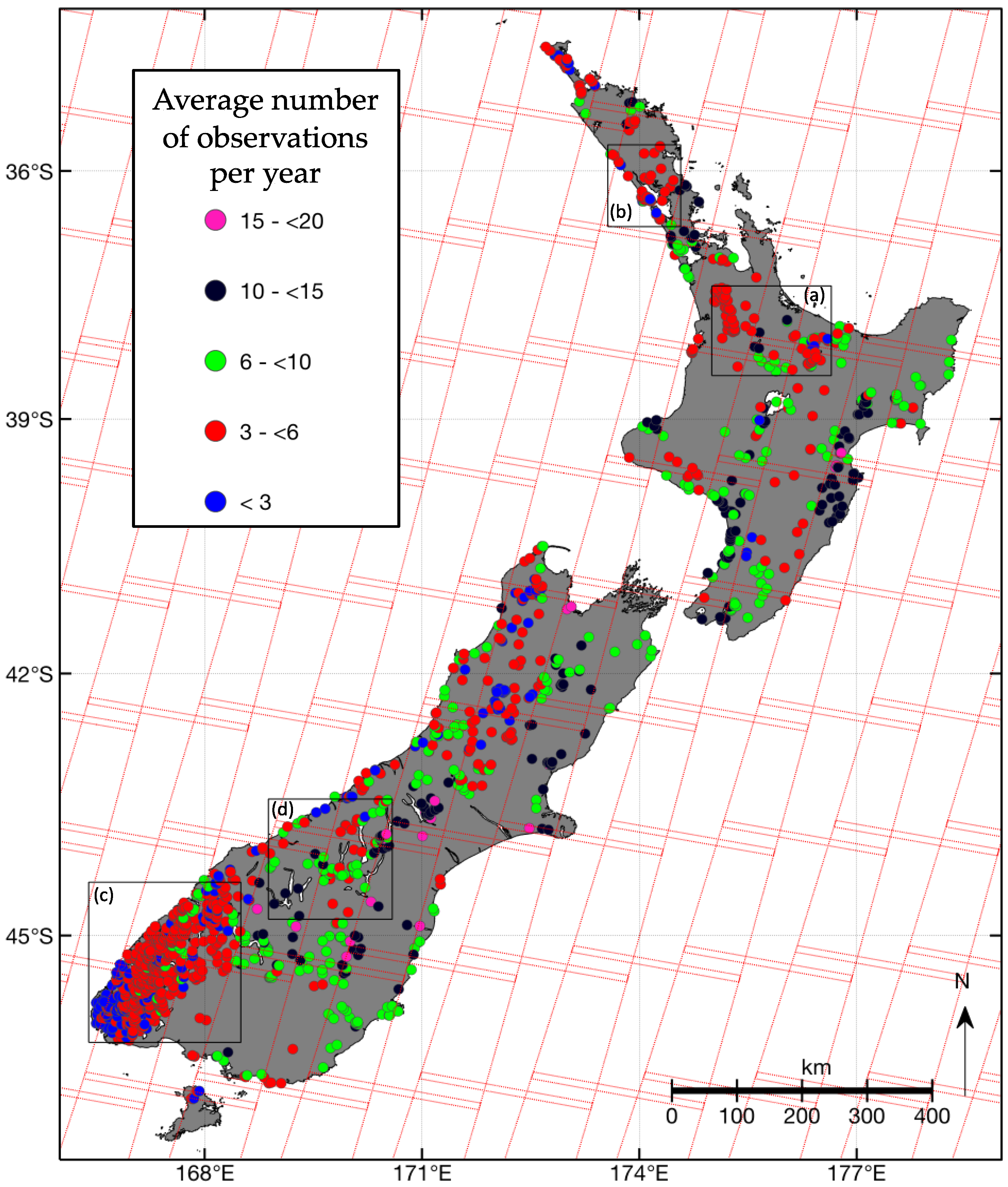
Landsat 8 data are acquired in 185 km swaths and segmented into 185 km × 180 km scenes that are defined in the second World-wide Reference System (WRS-2) of path (groundtrack parallel) and row (latitude parallel) coordinates (Figure 5) [33]. Adjacent paths overlap by approximately 56 km in the northern end of New Zealand and 76 km at the southern end. Every path is overpassed every 16 days and the path adjacent to it is overpassed seven days later. This means that repeat observations of certain parts of the country are possible every eight days and every 16 days in the remaining regions. Therefore, the maximum frequency of observations of any lake by Landsat 8 OLI is either 52 or 23 times per year, depending on its location with respect to the groundtrack of the orbital paths.
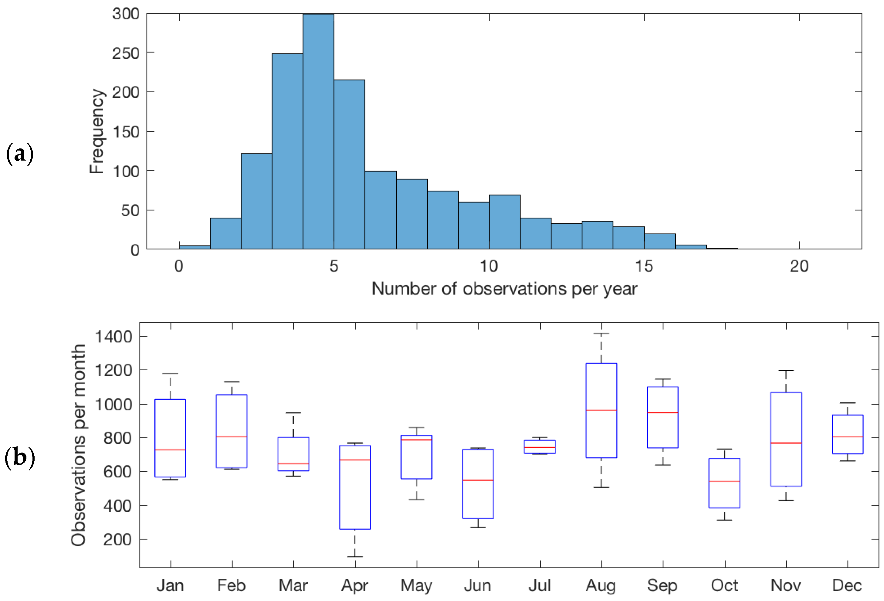
Successful imaging of aquatic ground targets by the OLI depends on cloudiness, and the quality of retrieval data is dependant on atmospheric conditions, such as haze, and reflection from the target surface, i.e., glint. Cloud cover varies greatly across New Zealand, with some areas of the country showing almost half as many sunshine hours as other regions [50,51]. Cloud masking, as described in the methods and removal of observations with reflectances outside the range between zero and one, produced 44,947 spectra for 1486 lakes across the country. The lakes in our data set are observed on average between once and 21 times per year. Lakes with four to six observations per year are most common and on avearge lakes are observed 6.3 times (Figure 6a). The median number of observations ranges between 600 and 1000 per month (Figure 6b). However, the interquartile range of the number of monthly observations shows that the highest number of successful retrievals occurs in January, February, August, and September, while April, May, June, and October can show the lowest number of data points.
The average annual number of images for each lake in the data set is shown on the map in Figure 5 (also available at lakes.takiwagis.co) along with the locations of the OLI ground paths. Lakes in areas of overlapping paths systematically show higher frequency of observations relative to lakes in non-overlapping areas, and variability in observation frequency within overlapping or non-overlapping ground path areas is consistent with statistics of sunshine hours [50]. For example, a small lake (lake ID 25550 in the FENZ geodatabase) near Nelson (41.27°S, 173.28°E), one of the sunniest cities in New Zealand, was observed successfully 20 times per year. Lakes in Hawkes Bay (39.49°S, 176.91°E) have high observation frequencies, as do lakes near Lake Tekapo (43.90°S, 170.53°E) in the central high country of the Canterbury region. Cloudiness is highest along the west coast of New Zealand, especially in Fjordland at the south-westernmost end of the South Island, which is being reflected by annual images fewer than four.
3.2. Correction for Purity
In Van der Woerd and Wernand [21,22], it was shown that in first approximation the hue angle can be reconstructed using a linear weighted sum of the band R(λ), in this case the four bands of OLI (see Equations (7)–(9)), and a correction Δα calculated by a fifth order polynomial (Figure 4a). Likewise, we calculated the difference in distance (S) from the white point between the hyperspectral and OLI results (ΔS). In Figure 4b, this difference is plotted as a function of the hue angle derived from the OLI bands and is approximated by the following fifth-order polynomial:
ΔS = −0.0099a5 + 0.1199a4 – 0.4594a3 + 0.7515a2 – 0.5095a + 0.1222
This equation is used to reconstruct the distance S and purity S* for all OLI spectra.
3.3. Lake Colour and Purity Distribution
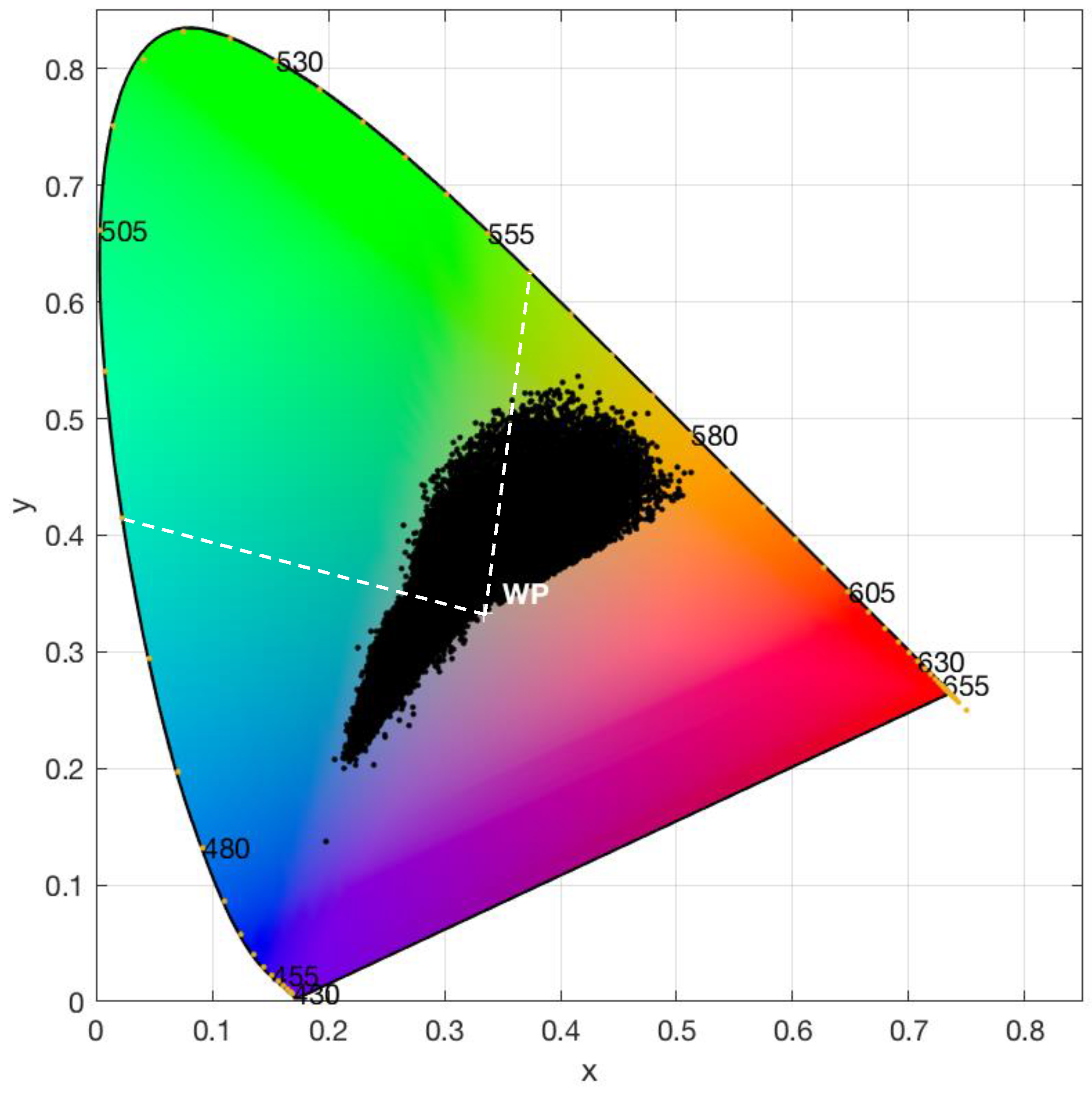
All 44,947 water colour observations from the study lakes, as derived by chromaticity analysis, are shown in Figure 7. The observations form a teardrop-shaped point cloud occupying predominantly orange-brown, yellow-green, and turquoise-blue areas of the colour space. The range of dominant wavelengths extends from 475 nm at the blue end of the spectrum to 585 nm at the yellow-orange end. Colour purity is strongest for observations in the orange-yellow part of the chromaticity diagram, as indicated by points over half way from the white point (x = y = 1/3) towards the locus. Colour purity of blue colours reaches 40% and blue-green to yellow-green colour purity is lower with a maximum of 20%.
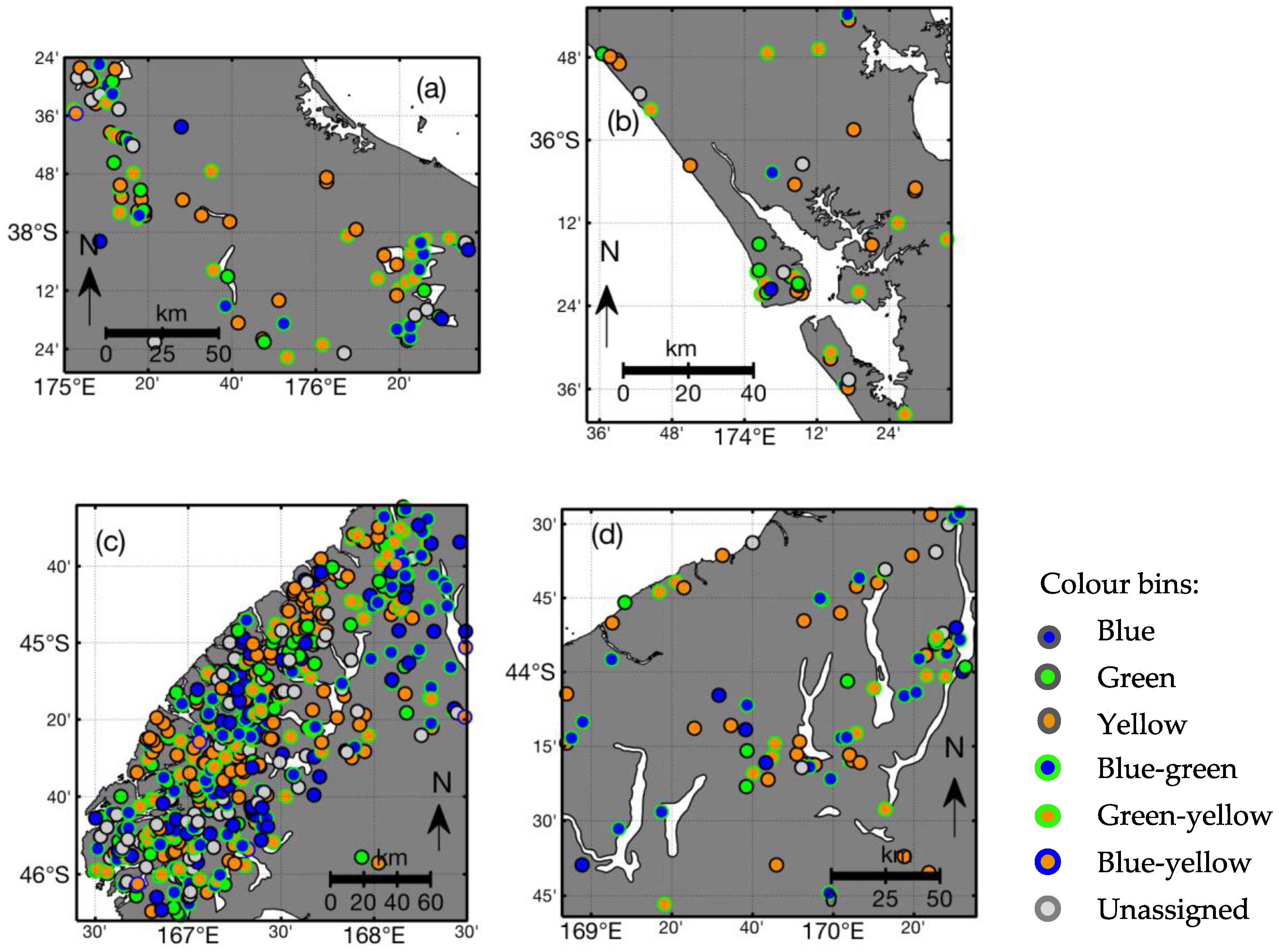
Observations of dominant wavelength show a bi-modal frequency distribution with most observations in the yellow-orange part of the spectrum, a secondary mode at the blue end and relatively fewer green observations (Figure 8a). This frequency distribution is sensitive to the spatial bias of observation frequency (Figure 5), and therefore it does not provide a representative summary of lake colour in New Zealand in general. Lake-mean dominant wavelength is more uniformly distributed (Figure 8b) than the individual observations, suggesting that colours are more or less equally represented at the lake level. The geographic distribution of mean dominant wavelength shows broad spatial patterns (Figure S1 in Supplementary Material; this dataset can also be explored at lakes.takiwa.co). For example, lakes in Fjordland, in the western half of the South Island of New Zealand tend to be blue to green (Figure 9c), while further north, in the Southern Alps, lakes are a mixture of deep blue to orange colours (Figure 9d). The North Island has many green lakes in the central volcanic plateau (southeastern corner of Figure 9a) and yellow to dark orange lakes in the peat-dominated landscape about 100 km northwest (northwest corner of Figure 9a). Lakes on the northern panhandle of the North Island are a diverse mix of blue to orange colours (Figure 9b).
Inspection of the distribution of dominant wavelength observations within lakes revealed that a large number of lakes are predominantly blue or predominantly yellow-orange, but there are no lakes that are only green (Figure 10). Lakes that are green on average typically show observations across the entire spectrum. For example, Lake Rotomanuka, a eutrophic peat lake of 8 m maximum depth in an agricultural catchment [52], is persistently orange with a mean dominant wavelength of 575 nm and purity from 13 to 80% (Figure 11). Lake Pukaki is a glacial lake fed by cold, short-transit-time rivers with little interaction with vegetated terrain [26]. It is ultra-oligotrophic and famous for its turquoise-blue water that is due to inputs of fine, highly scattering, and weakly absorbing glacial ‘flour’ [1]. The dominant wavelength of Lake Pukaki varies little (485–513 nm with a mean 494 nm) and its purity ranges from 3 to 36% (mean 19%) (Figure 11). A lake with markedly variable colour is Lake Rotoiti. This monomictic, eutrophic volcanic lake has a maximum depth of 124 m [53] and it shows seasonal variability in the time series of dominant wavelength ranging from 490 to 571 nm (mean of 521 nm). Colour purity ranges from 5 to 46% with high values coinciding with maxima in dominant wavelength (Figure 11). This pattern is likely caused by seasonal blooms of picocyanobacteria [54], during which chl a concentrations typically reach 10 mg m−3.
To facilitate a broad classification of the study lakes, the full spectrum of dominant wavelength was divided into five colour bins: three solid colours (blue: λd < 495, green: 495 ≤ λd < 560, and yellow: λd ≥ 560 nm) and three transient bins (blue-green, yellow-green, blue-yellow). Lakes were assigned a solid colour if 60% or more observations of dominant wavelength were within the range of a single solid colour. Lakes with bimodal distributions of dominant wavelength were identified as transient based on the distribution of observations between solid colour ranges, as listed in Table 1. Due to the relative sparseness of green observations, transient greenness required a minimum of 20% of green observations only. The numbers of blue, blue-green, and green-yellow lakes are similar (16%, 19%, 21%, respectively) and only 8% of lakes are predominantly green. 15% of lakes do not fit into one of those colour bins because their variability in dominant wavelength does not fit this categorisation.
Figure 12 shows the geographic distribution of lake colours by bins in regions, as identified in Figure 5 (Figure S2 in Supplementary Material shows the entire study area). The differences between the lake-specific mean dominant wavelength (Figure 9) and the colour bin shows that the mean statistic is a poor descriptor of lake colour over the observation period for about 40% of lakes due to their bi-modal frequency distribution of dominant wavelength. Hence, more lakes have an average dominant wavelength in the green part of the spectrum in Figure 9 than expected from the minimum of the frequency distribution of observations (Figure 8a), and Figure 12 shows that the green colour is an artefact of averaging over observations in the blue and yellow range of the spectrum.
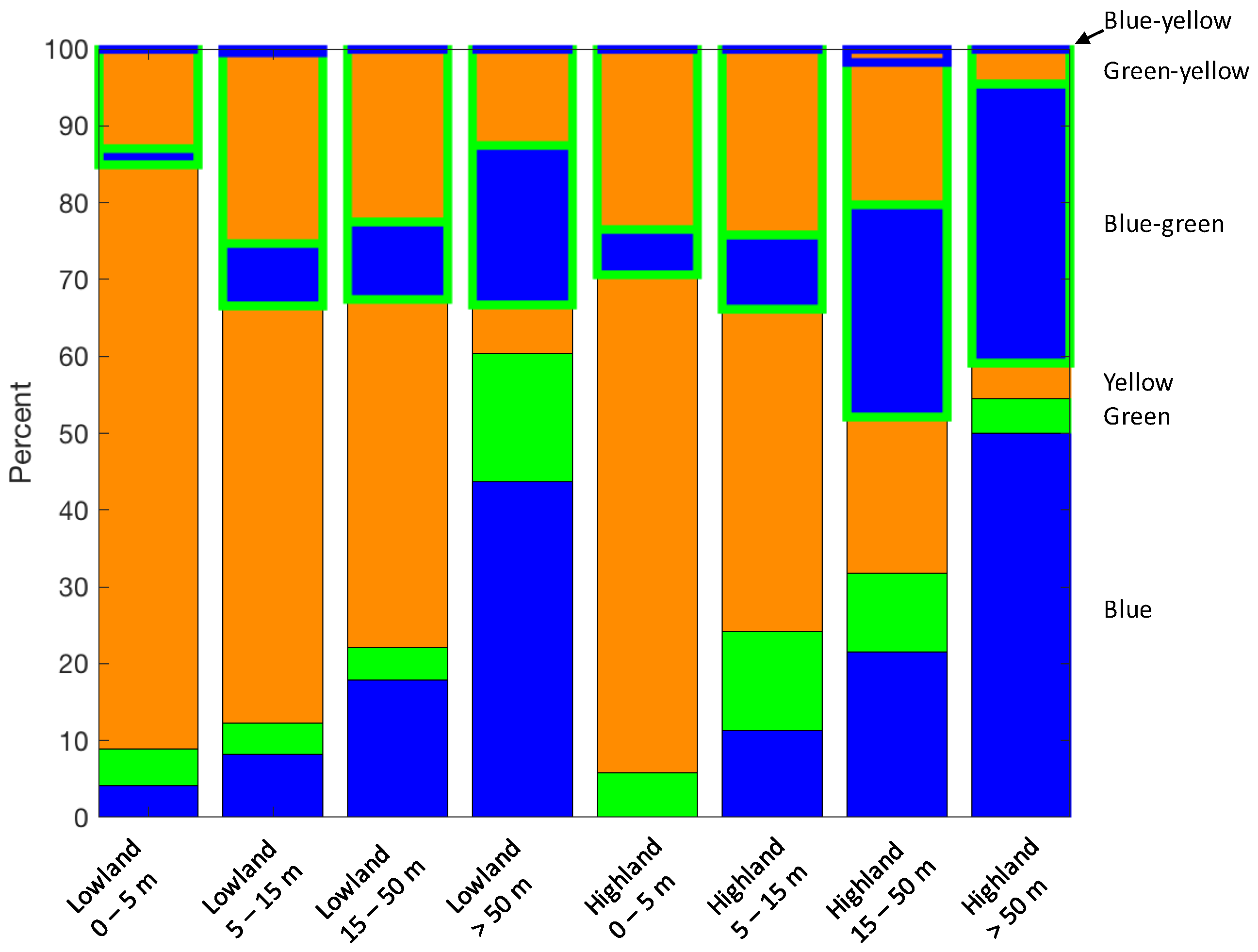
Broad geographic patterns in lake colour-bin distribution exist (Figure 12), which are consistent with geomorphic and land use characteristics. For example, blue lakes occur in the more sparsely populated, mountainous, and forested regions along the west coast of the South Island (Figure 12c) and in the eastern portion of the North Island (southeast corner of Figure 12a). Yellow and green-yellow lakes dominate in the agricultural areas in the central North Island and the southeast of the South Island. A large number of yellow lakes also occur along the South Island’s west coast where there are many lakes in forest catchments with high CDOM inputs. These geographical patterns can be partly explained by elevation and lake depth. Figure 13 shows that systematic differences in lake colour exist between eight classes of lowland and highland lakes of different depths. Approximately 85% of shallow lakes (<5 m deep) in lowlands are yellow and about 10% are transient yellow-green lakes. The fraction of blue and green lakes increases with lake depth in lowland lakes, and deep lakes (>50 m) are often blue or blue-green transient. At higher elevations, the proportion of yellow lakes is smaller than in lowland lakes, and the proportion of blue and blue-green lakes increases with lake depth.
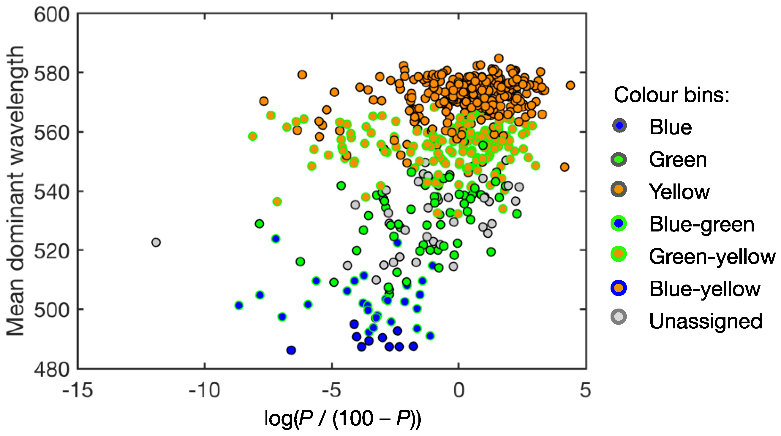
568 of our study lake catchments contain high-producing exotic grassland and percentage cover of this land-use reaches over 90% for many lakes. The relationship between mean dominant wavelength and the transformed percent cover forms a point cloud with a distinct boundary, showing that there are no blue or blue-green lakes in catchments with over 25% (transformed value of −1.1) high-producing exotic grassland (Figure 14). Yellow and green-yellow transient (see definitions in Table 1) lakes mostly have catchments with this cover type making up more than 25%.
4. Discussion
In this study, we determined the observation frequency by Landsat 8 OLI and the colour of 1486 lakes across New Zealand. Monitoring of the health and water quality of this resource falls to the country’s sixteen local governments (i.e., regional councils) [55]. This involves in-situ sampling for a base set of water quality attributes (chlorophyll a, total nitrogen, and total phosphorus) and additional attributes, as decided by the regional councils [56]. A recent summary of council data indicated that 63% of the monitored lakes are mesotrophic, eutrophic, or supertrophic and 36.7% of lakes showed degrading trends. However, these assessments were limited to 72 lakes for state and even fewer (18 lakes) for the trend analysis [29], and therefore, these results are hardly representative of the nation’s lakes in general. We demonstrate that even with the requirement for clear skies and relatively infrequent revisits (every eight or 16 days), Landsat 8 OLI can resolve 1486 lakes and over 50% of these lakes are successfully observed four or more times per year. Higher observation frequencies should be achieved by similar currently operational multispectral sensors with shorter revisit periods e.g., by the Multispectral Instrument (MSI) on the tandem mission Sentinel-2 a and b of the European Space Agency with a revisit period of three to four days [57].
Despite the advantages of enhanced spatio-temporal coverage of satellite observations of lakes, remote sensing is unlikely to provide biogeochemical quantities for current regulatory monitoring programmes, because prediction-precision residuals relative to in situ samples are relatively large. These residuals are caused by the difficulty of retrieving concentrations of independently varying optically active substances in inland waters and spatio-temporal variations of IOPs, which hamper the application of algorithms across a wide range of optical water types such as those found in New Zealand. Lake colour estimation from satellite imagery provides a reliable synoptic measurement of an ecosystem attribute, as it does not suffer from our limited knowledge of IOPs of optically active constituents in the water.
As we expected from our knowledge of New Zealand lakes, our dataset covers a large range of natural water colours and we look forward to comparable large-scale studies to fully define the global boundaries of the point cloud in the chromaticity diagram (Figure 7). As an initial attempt to handle the diversity of lake colour, we defined a simple heuristic classification of lakes into colour bins (Table 1), which aimed to capture the mean properties and identify cases where mean properties poorly represent lake state. With this approach we characterised both water type (colour of individual observations) and lake type (i.e., colour bin membership). The colour of individual observations may be useful for algorithm selection in multi-algorithm approaches to inland water applications [58] and the colour-bin classification relates a lake to its environment, facilitating further ecological studies of the drivers of lake water quality at a range of spatial scales. Other classifications of optical water types were typically designed using in-situ hyperspectral data and in-situ optically active constituents e.g., [59,60]. When applying these classifications to satellite data, misclassifications may occur due to the reduced information content of multispectral data relative to the hyperspectral in-situ reflectances. Our approach is solely based on multispectral satellite data and quantifying the limitations that this imposes on algorithm selection and water quality monitoring is the goal of ongoing validation of remotely sensed water colour with in-situ hyperspectral and water quality data.
The colour of water is directly linked to the spectral quality of the underwater light field and therefore the light available for photosynthesis by aquatic plants and visibility for the aquatic fauna [4,61]. The relationship between water colour and inherent optical properties of water quality constituents should allow for colour to be used as proxy for concentrations of chl a, CDOM, or SPM in well-characterised systems. This provides an opportunity for efficient monitoring using stationary or remote radiometers, as well as for community involvement in science, e.g., through the measurement of colour by smartphone cameras [62]. In addition, the perceived colour has been directly linked to recreational use and the desirability of freshwater systems [2,3] affecting the social and economic value of lakes and rivers [63]. This makes perceived colour a useful measurement in the context of optical water quality [1,4] and led to its recent inclusion in the New Zealand national environmental monitoring standards for lakes [64]. One example application is the protection of visual characteristics of the unique and iconic natural character of lakes, such as Tekapo and Pukaki of the Canterbury region, which have low clarity and distinctive milky-blue hues. To this end, water colour monitoring based on the Munsell colour scale [65] has been part of regional water quality objectives [66]. However, only 41 of the region’s 464 lakes that are greater than 1 ha are monitored and the high country lakes, including the aforementioned optically unique lakes, are sampled by helicopter, prohibiting visual Munsell colour matching. Our dataset includes 157 Canterbury lakes and immediately offers four years of data that can be used to set targets for water colour and assess departures from baseline values and trends. The relationships that we described between lake colour and catchment land use, lake elevation, and depth suggest that colour can be predicted from a suitable set of driver variables and future effort will be devoted to finding these relationships.
A previous multivariate analysis identified percentage land cover by high-producing exotic grassland as the strongest predictor whether a lake shifted from clear to turbid states [67] and we therefore chose this variable for a first investigation into potential correlates of lake water colour. High-producing exotic grassland identifies pasture used for intensive dairy, beef, and sheep grazing, which is the mainstay of New Zealand’s primary industry. Covering almost 9 mil ha, it made up 33% of New Zealand’s land area in 2012 and it had the second highest increase in areal coverage between 2008 and 2012 after harvested forest [48,68]. Nitrogen and phosphorus runoff from fertiliser application and animal excretion has been identified as a leading cause for the degradation in New Zealand’s inland waters [69,70]. Our results show that lakes with a higher proportion of high-producing exotic grassland are more green to orange, rather than blue and blue-green (Figure 14). If lake colour is taken as a proxy for chl a and SPM, this relationship supports the causal link suggested between dairy production and environmental impacts [68]. However, blue lakes also tend to be deep, which makes them less vulnerable to eutrophication and at high elevation (Figure 13), i.e., in landscapes potentially less suitable for intensive-pasture farming. The observed correlation must therefore be examined comprehensively with other factors and the present analysis is merely the first step towards an explanatory multivariate prediction model for lake water colour.
Limitations of Our Approach
Our approach of restricting remote sensing data to a 90 by 90 m AOI per lake limits the results in at least two ways. First, it reduces the image yield under partially cloudy conditions where data was rejected from the lake centroid, but valid data could have been retrieved from the lake at a different location. Second, we average over spatial variability at scales below 90 m and neglect variability at larger scales. Many of our study lakes show considerable variability in optically active substances at a range of scales [71,72,73,74] and systematic gradients are common along hydrologic or topographic boundaries. We accept these limitations for the benefit that reduced data volume and dimensionality offers to processing and interpreting data on over a thousand targets.
The surface reflectance product used in this study (ρ) was designed as a land reflectance product and is not corrected for sun glint and adjacency effects, which may affect our colour estimate in some situations. However, the effect of glint has no wavelength dependence [36] and the spectral effect of whitecaps is weak [37]. Therefore, these contributions have no or little intrinsic colour, and can thus be approximated by the addition of a constant term to all four bands in our Equations (7) and (8). This addition will have an effect on purity, but not on dominant wavelength. Other investigators have also found the surface reflectance product to be a reasonable choice for water pixels [35,75]. In particular, Pahlevan et al. (2017) [76] wrote that ρ is expected to have seemingly reasonable radiometric properties over small inland bodies of water, and Bernardo et al. (2017) [77] found that using ρ outperforms reflectance products from several other atmospheric correction methods in TSS retrieval in a Brazilian reservoir. Our results for Lake Pukaki support this (Figure 11). Lake Pukaki is a blue lake with stable water colour over the years, and indeed, the dominant wavelength remains remarkably stable around 495 nm in 25 scenes. Purity does change however, and in the future it would be interesting if this purity change can be coupled to viewing geometry or wind effects. We chose to use ρ from the Tier 1 collection Landsat data, because one of our main objectives is to demonstrate the monitoring capability of chromaticity analysis using a readily available data product that is easy to obtain by non-research users, such as government water resources scientists. Most aquatic remote sensing studies use remote sensing reflectance, which has sun and sky glint contributions removed by atmospheric correction methods that are designed for ocean colour applications [76,78]. Developing better atmospheric correction of inland and coastal targets is an active area of research and there is currently no consensus as to the best method [76,77,79]. To see whether atmospheric correction developed for aquatic targets improves our analysis, we processed five of our Landsat 8 scenes using SeaDAS with default settings, as described in [76,80]. We found that about half of the SeaDAS-calculated remote sensing reflectances were negative, leading to unrealistic values for dominant wavelength and purity. Therefore, we conclude that the standard USGS surface reflectance product is at this stage a suitable choice for demonstrating the application and feasibility of large-scale lake colour monitoring. In future work, we aim to quantify the difference between ρ-based chromaticity and remote-sensing-reflectance-based chromaticity and to exploit the great optical diversity of New Zealand lakes to improve atmospheric correction methods.
Landsat 8 OLI is not the ideal sensor to reconstruct the full spectrum of visible light of water-leaving radiance, because it has only four spectral bands with relatively wide bandpasses [41]. The Moderate Resolution Imaging Spectroradiometer (MODIS on Terra and Aqua) and the Ocean and Land Colour Instrument (OLCI on Sentinel-3) with their larger number of spectral bands at narrower bandpasses, are more accurate in the estimation of hue angles when compared with OLI [21,22]. The reconstruction of purity had previously been more limited. At all wavelengths, the expression of the colour is less pronounced in the OLI product, resulting in an offset of order 0.005 for angles below 80°, up to 0.05 for the bluest waters with hue angles near 230°. This is to be expected, because the broad band integration of radiation will always result in the loss of dominant wavelength expression. Nevertheless, the real distance can be reconstructed reasonably well by adding the results from Equation (13) (Figure 7 shows the resulting positions in the chromaticity diagram for all OLI spectra). Thus, we agree with van der Woerd and Wernand [22] that OLI is remarkably successful in the retrieval of the colour of water reflectance spectra and we chose to use this sensor due to its better spatial resolution compared with MODIS and OLCI and the decades-long continuity of the Landsat programme [81]. Future efforts will be directed toward the analysis of the merged time series from the Thematic Mapper (Landsat 5), Enhanced Thematic Mapper (Landsat 7), and OLI to establish a lake colour library for the study of drivers, trends, and resilience of the optical water quality of New Zealand lakes.
5. Conclusions
Water colour is an intuitive water quality attribute that can be measured by satellite sensors without requiring knowledge of inherent optical properties. It is intrinsically linked to other important water quality attributes such as clarity, the concentration of phytoplankton, suspended matter and CDOM, and is therefore a useful integrating measure of ecosystem health, as well as an attribute that can be managed in its own right. We establish a methodology for satellite-based measurement of water colour and outline future applications through a preliminary exploration of this data set against land-use characteristics and depth-elevation classes. Our four-year water colour time series and summary statistics for almost 40% of New Zealand lakes represents the first observation-based assessment of a lake water quality attribute at the national scale and we suggest that geologic, anthropogenic, climatic and physiographic predictors may be used to understand contemporary relationships between driving factors and lake colour.
Supplementary Materials
The following are available online at https://www.mdpi.com/2072-4292/10/8/1273/s1, Figure S1: Geographic distribution of lakes coloured by mean dominant wavelength. The boxes (a) to (d) show the locations of the closeup maps of Figure 9 and Figure 12. Figure S2: Geographic distribution of lakes coloured by colour bins according to Table 1 boxes (a) to (d) show the locations of the closeup maps of Figure 9 and Figure 12.
Author Contributions
Conceptualization, M.K.L.; Methodology, M.K.L., U.N. and M.A.; Formal Analysis, M.K.L., H.J.W.; Data Curation, U.N.; Writing—Original Draft Preparation, M.K.L.; Writing—Review & Editing, U.N., M.A., H.J.v.d.W.; Project Administration, M.K.L.
Funding
This research was funded by the New Zealand Ministry for Business, Employment and Innovation grant number UOWX1503.
Acknowledgments
This work is part of the Lakes Resilience Research Programme as identified in the funding section above, and the authors would like to acknowledge valuable discussion and feedback from the other key investigators of that programme. Julia King (summer research scholarship recipient 2016/17) is thanked for early exploration and mapping of the colour data set and Ray Littler provided very insightful statistical advice. The manuscript was improved by editorial corrections and suggestions by Fiona Martin and through very helpful and insightful comments from three anonymous reviewers.
Conflicts of Interest
The authors declare no conflict of interest.
References
- Davies-Colley, R.J.; Vant, W.N.; Smith, D.G. Colour and Clarity of Natural Waters—Science and Management of Optical Water Quality; The Blackburn Press: Caldwell, NJ, USA, 1993. [Google Scholar]
- Smith, D.G.; Davies-Colley, R.J. Perception of water clarity and colour in terms of suitability for recreational use. J. Environ. Manag. 1992, 36, 225–235. [Google Scholar] [CrossRef]
- West, A.O.; Nolan, J.M.; Scott, J.T. Optical water quality and human perceptions of rivers: An ethnohydrology study. Ecosyst. Health Sustain. 2016, 2. [Google Scholar] [CrossRef]
- Kirk, J.T.O. Optical Water-Quality—What Does It Mean and How Should We Measure It. J. Water Pollut. Con. F 1988, 60, 194–197. [Google Scholar]
- Wyszecki, G.; Stiles, W.S. Color Science: Concepts and Methods, Quantitative Data, and Formulae, 2nd ed.; Wiley-Interscience: Hoboken, NJ, USA, 2000. [Google Scholar]
- CIE. Commission Internationale de l’Éclairage Proceedings; Cambridge University Press: Cambridge, UK, 1932. [Google Scholar]
- Kirk, J.T.O. Light & Photosynthesis in Aquatic Ecosystems, 2nd ed.; Cambridge University Press: Cambridge, UK, 1994. [Google Scholar]
- Mobley, C.D. Light and Water: Radiative Transfer in Natural Waters; Academic Press: Cambridge, MA, USA, 1994. [Google Scholar]
- IOCCG. Remote Sensing of Inherent Optical Properties: Fundamentals, Tests of Algorithms, and Applications. In Reports of the International Ocean-Colour Coordinating Group (IOCCG); IOCCG: Dartmouth, NS, Canada, 2006. [Google Scholar]
- Pope, R.M.; Fry, E.S. Absorption spectrum (380–700 nm) of pure water. II. Integrating cavity measurements. Appl. Opt. 1997, 36, 8710–8723. [Google Scholar] [CrossRef] [PubMed]
- Bukata, R.P.; Bruton, J.E.; Jerome, J.H. Use of Chromaticity in Remote Measurements of Water-Quality. Remote Sens. Environ. 1983, 13, 161–177. [Google Scholar] [CrossRef]
- Bukata, P.R.; Jerome, J.H.; Kondratyev, K.Y.; Pozdnyakov, D. Optical Properties and Remote Sensing of Inland and Coastal Waters; CRC Press: Boca Raton, FL, USA, 1995. [Google Scholar]
- Dekker, A.G.; Peters, S.W.M.; Vos, R.J.; Rijkeboer, M. Remote sensing for inland water quality detection and monitoring: State-of-the-art application in Friesland. In GIS and Remote Sensing techniques in Land-and Water-Management; Dijk, A.v., Bos, M.G., Eds.; Kluwer Academic Publishers: Alphen aan den Rijn, The Netherlands, 2001; pp. 17–38. [Google Scholar]
- Julian, J.P.; Davies-Colley, R.J.; Gallegos, C.L.; Tran, T.V. Optical water quality of inland waters: A landscape perspective. Ann. Assoc. Am. Geogr. 2013, 103, 309–318. [Google Scholar] [CrossRef]
- Gholizadeh, M.H.; Melesse, A.M.; Reddi, L. A Comprehensive Review on Water Quality Parameters Estimation Using Remote Sensing Techniques. Sensors 2016, 16, 1298. [Google Scholar] [CrossRef] [PubMed]
- Palmer, S.C.J.; Kutser, T.; Hunter, P.D. Remote sensing of inland waters: Challenges, progress and future directions. Remote Sens. Environ. 2015, 157, 1–8. [Google Scholar] [CrossRef] [Green Version]
- Tyler, A.N.; Hunter, P.D.; Spyrakos, E.; Groom, S.; Constantinescu, A.M.; Kitchen, J. Developments in Earth observation for the assessment and monitoring of inland, transitional, coastal and shelf-sea waters. Sci. Total Environ. 2016, 572, 1307–1321. [Google Scholar] [CrossRef] [PubMed] [Green Version]
- Allan, M.G. Remote Sensing of Water Quality in Rotorua and Waikato Lakes. Master’s Thesis, University of Waikato, Hamilton, New Zealand, 2008. [Google Scholar]
- Odermatt, D.; Gitelson, A.; Brando, V.E.; Schaepman, M. Review of constituent retrieval in optically deep and complex waters from satellite imagery. Remote Sens. Environ. 2012, 118, 116–126. [Google Scholar] [CrossRef] [Green Version]
- Olmanson, L.G.; Bauer, M.E.; Brezonik, P.L. A 20-year Landsat water clarity census of Minnesota’s 10,000 lakes. Remote Sens. Environ. 2008, 112, 4086–4097. [Google Scholar] [CrossRef]
- Van der Woerd, H.J.; Wernand, M.R. True Colour Classification of Natural Waters with Medium-Spectral Resolution Satellites: SeaWiFS, MODIS, MERIS and OLCI. Sensors 2015, 15, 25663–25680. [Google Scholar] [CrossRef] [Green Version]
- Van der Woerd, J.H.; Wernand, R.M. Hue-Angle Product for Low to Medium Spatial Resolution Optical Satellite Sensors. Remote Sens. 2018, 10, 180. [Google Scholar] [CrossRef]
- Lowe, D.J.; Green, J.D. The basis for lake diversity: Origins and development of lakes. In Inland Waters of New Zealand; Viner, A.B., Ed.; DSIR Science Publishing Centre: Wellington, New Zealand, 1987; p. 494. [Google Scholar]
- Vant, W.N.; Davies-Colley, R.J. Factors affecting clarity of New-Zealand lakes. New Zeal. J. Mar. Fresh. 1984, 18, 367–377. [Google Scholar] [CrossRef]
- Davies-Colley, R.J.; Vant, W.N. Absorption of light by yellow substance in fresh-water lakes. Limnol. Oceanogr. 1987, 32, 416–425. [Google Scholar] [CrossRef]
- Gallegos, C.L.; Davies-Colley, R.J.; Gall, M. Optical closure in lakes with contrasting extremes of reflectance. Limnol. Oceanogr. 2008, 53, 2021–2034. [Google Scholar] [CrossRef] [Green Version]
- Leathwick, J.R.; West, D.; Gerbeaux, P.; Kelly, D.; Robertson, H.; Bronwn, D.; Chadderton, W.L.; Ausseil, A.G. Freshwater Ecosystems of New Zealand (FENZ) Geodatabase Version One—User Guide; NIWA: Hamilton, New Zealand, 2010. [Google Scholar]
- Snelder, T. Definition of a Multivariate Classification of New Zealand Lakes; National Institute of Water and Atmospheric Research: Christchurch, New Zealand, 2006. [Google Scholar]
- Larned, S.; Snelder, T.; Unwin, M.; McBride, G.B.; Verburg, P.; McMillan, H. Analysis of Water Quality in New Zealand Lakes and Rivers; National Institute of Water and Atmospheric Research: Christchurch, New Zealand, 2015. [Google Scholar]
- Burns, N.M.; Rutherford, J.C.; Clayton, J.S. A Monitoring and Classification System for New Zealand Lakes and Reservoirs. Lake Reserv. Manag. 1999, 15, 255–271. [Google Scholar] [CrossRef]
- Verburg, P.; Hamill, K.; Unwin, M.; Abell, J. Lake Water Quality in New Zealand 2010: Status and Trends; National Institute of Water and Atmospheric Research: Christchurch, New Zealand, 2010. [Google Scholar]
- LINZ Land Information New Zealand—Aerial Imagery. Sourced from the LINZ Data Service and Licensed by the Copyright Holder for Re-Use under the Creative Commons Attribution 3.0 New Zealand. Available online: https://data.linz.govt.nz/ (accessed on 13 August 2018).
- Roy, D.P.; Wulder, M.A.; Loveland, T.R.; Woodcock, C.E.; Allen, R.G.; Anderson, M.C.; Helder, D.; Irons, J.R.; Johnson, D.M.; Kennedy, R.; et al. Landsat-8: Science and product vision for terrestrial global change research. Remote Sens. Environ. 2014, 145, 154–172. [Google Scholar] [CrossRef]
- USGS. Product Guide—Landsat 8 Surface Reflectance Code (LaSRC) Product, Version 4.3 2018. Available online: https://landsat.usgs.gov/sites/default/files/documents/lasrc_product_guide.pdf (accessed on 13 August 2018).
- Vermote, E.; Justice, C.; Claverie, M.; Franch, B. Preliminary analysis of the performance of the Landsat 8/OLI land surface reflectance product. Remote Sens. Environ. 2016, 185, 46–56. [Google Scholar] [CrossRef]
- Kay, S.; Hedley, D.J.; Lavender, S. Sun Glint Correction of High and Low Spatial Resolution Images of Aquatic Scenes: A Review of Methods for Visible and Near-Infrared Wavelengths. Remote Sens. 2009, 1, 697–730. [Google Scholar] [CrossRef]
- Nicolas, J.M.; Deschamps, P.Y.; Frouin, R. Spectral reflectance of oceanic whitecaps in the visible and near infrared: Aircraft measurements over open ocean. Geophys Res. Lett. 2001, 28, 4445–4448. [Google Scholar] [CrossRef] [Green Version]
- Zhu, Z.; Wang, S.; Woodcock, C.E. Improvement and expansion of the Fmask algorithm: Cloud, cloud shadow, and snow detection for Landsats 4–7, 8, and Sentinel 2 images. Remote Sens. Environ. 2015, 159, 269–277. [Google Scholar] [CrossRef]
- Foga, S.; Scaramuzza, P.L.; Guo, S.; Zhu, Z.; Dilley, R.D.; Beckmann, T.; Schmidt, G.L.; Dwyer, J.L.; Joseph Hughes, M.; Laue, B. Cloud detection algorithm comparison and validation for operational Landsat data products. Remote Sens. Environ. 2017, 194, 379–390. [Google Scholar] [CrossRef] [Green Version]
- McFeeters, S.K. The use of the Normalized Difference Water Index (NDWI) in the delineation of open water features. Int. J. Remote Sens. 1996, 17, 1425–1432. [Google Scholar] [CrossRef]
- Barsi, J.; Lee, K.; Kvaran, G.; Markham, B.; Pedelty, J. The Spectral Response of the Landsat-8 Operational Land Imager. Remote Sens. 2014, 6, 10232–10251. [Google Scholar] [CrossRef] [Green Version]
- Pahlevan, N.; Lee, Z.P.; Wei, J.W.; Schaaf, C.B.; Schott, J.R.; Berk, A. On-orbit radiometric characterization of OLI (Landsat-8) for applications in aquatic remote sensing. Remote Sens. Environ. 2014, 154, 272–284. [Google Scholar] [CrossRef]
- Alföldi, T.T.; Munday, J.C. Water quality analysis by digital chromaticity mapping of Landsat data. Can. J. Remote Sens. 1978, 4, 108–126. [Google Scholar] [CrossRef]
- Munday, J.C. Chromaticity of path radiance and atmospheric correction of Landsat data. Remote Sens. Environ. 1983, 13, 525–538. [Google Scholar] [CrossRef]
- Mobley, C.D. Hydrolight Users’ Guide. 2013. Available online: https://www.sequoiasci.com/wp-content/uploads/2013/07/HE52UsersGuide.pdf (accessed on 10 August 2018).
- IOCCG Synthesized Dataset from IOCCG Report 5. 2015. Available online: http://ioccg.org/what-we-do/ioccg-publications/ioccg-reports/synthesized-dataset-from-ioccg-report-5/ (accessed on 10 August 2018).
- USGS. USGS Spectral Viewer. 2018. Available online: https://landsat.usgs.gov/using-usgs-spectral-viewer (accessed on 10 August 2018).
- Landcare. Land Cover Database Version 4.1, Mainland New Zealand. Landcare Research: 2015. Available online: https://lris.scinfo.org.nz/layer/48423-lcdb-v41-land-cover-database-version-41-mainland-new-zealand/ (accessed on 10 August 2018).
- Tait, A.; Liley, B. Interpolation of daily solar radiation for New Zealand using a satellite data-derived cloud cover surface. Weather Clim. 2009, 29, 70–88. [Google Scholar]
- NIWA. Sunshine Hours Annual Average 1972–2013. Available online: https://statisticsnz.shinyapps.io/sunshine_hours/ (accessed on 10 August 2018).
- Dean-Speirs, T.; Neilson, K. Waikato Region Shallow Lakes Management Plan. 2014. Available online: https://www.waikatoregion.govt.nz/services/publications/technical-reports/tr/tr201458 (accessed on 10 August 2018).
- Von Westernhagen, N.; Hamilton, D.P.; Pilditch, C.A. Temporal and spatial variations in phytoplankton productivity in surface waters of a warm-temperate, monomictic lake in New Zealand. Hydrobiologia 2010, 652, 57–70. [Google Scholar] [CrossRef] [Green Version]
- Wood, S.A.; Paul, W.J.; Hamilton, D.P. Cyanobacterial Biovolumes for the Rotorua Lakes. 2008. Available online: https://www.boprc.govt.nz/media/32233/Cawthron-090803-CyanobacterialbiovolumesforRotorualakes.pdf (accessed on 10 August 2018).
- USGS. Path/Row Shapefiles. 2018. Available online: https://landsat.usgs.gov/pathrow-shapefiles (accessed on 10 August 2018).
- Ministry for the Environment. A Guide to the National Policy Statement for Freshwater Management 2014; MfE: Wellington, New Zealand, 2015.
- Ministry for the Environment. National Policy Statement for Freshwater Management 2014; MfE: Wellington, New Zealand, 2014.
- Drusch, M.; Del Bello, U.; Carlier, S.; Colin, O.; Fernandez, V.; Gascon, F.; Hoersch, B.; Isola, C.; Laberinti, P.; Martimort, P.; et al. Sentinel-2: ESA’s Optical High-Resolution Mission for GMES Operational Services. Remote Sens. Environ. 2012, 120, 25–36. [Google Scholar] [CrossRef]
- Moore, T.S.; Dowell, M.D.; Bradt, S.; Ruiz Verdu, A. An optical water type framework for selecting and blending retrievals from bio-optical algorithms in lakes and coastal waters. Remote Sens. Environ. 2014, 143, 97–111. [Google Scholar] [CrossRef] [PubMed] [Green Version]
- Spyrakos, E.; O’Donnell, R.; Hunter, P.D.; Miller, C.; Scott, M.; Simis, S.G.H.; Neil, C.; Barbosa, C.C.F.; Binding, C.E.; Bradt, S.; et al. Optical types of inland and coastal waters. Limnol. Oceanogr. 2017, 63, 846–870. [Google Scholar] [CrossRef] [Green Version]
- Eleveld, A.M.; Ruescas, B.A.; Hommersom, A.; Moore, S.T.; Peters, W.S.; Brockmann, C. An Optical Classification Tool for Global Lake Waters. Remote Sens. 2017, 9, 420. [Google Scholar] [CrossRef]
- Karlsson, J.; Byström, P.; Ask, J.; Ask, P.; Persson, L.; Jansson, M. Light limitation of nutrient-poor lake ecosystems. Nature 2009, 460, 506. [Google Scholar] [CrossRef] [PubMed]
- Busch, J.A.; Price, I.; Jeansou, E.; Zielinski, O.; van der Woerd, H.J. Citizens and satellites: Assessment of phytoplankton dynamics in a NW Mediterranean aquaculture zone. Int. J. Appl. Earth Obs. 2016, 47, 40–49. [Google Scholar] [CrossRef]
- Brauman, K.A.; Daily, G.C.; Duarte, T.K.e.; Mooney, H.A. The Nature and Value of Ecosystem Services: An Overview Highlighting Hydrologic Services. Annu. Rev. Environ. Resour. 2007, 32, 67–98. [Google Scholar] [CrossRef]
- MfE. National Environmental Monitoring Standards—Water Quality, Part 3 (Draft). Ministry for Business, Innovation and Employment, 2017. Available online: http://nems.org.nz/documents/water-quality-part-3-lakes/ (accessed on 10 August 2018).
- Davies-Colley, R.J.; Smith, D.G.; Speed, D.J.; Nagels, J.W. Matching natural water colors to Munsell standards. J. Am. Water Resour. Assoc. 1997, 33, 1351–1361. [Google Scholar] [CrossRef]
- Hayward, S.; Meredith, A.; Stevenson, M. Review of Proposed NRRP Water Quality Objectives and Standards for Rivers and Lakes in the Canterbury Region; Environment Canterbury: Christchurch, New Zealand, 2009.
- Schallenberg, M.; Sorrell, B. Regime shifts between clear and turbid water in New Zealand lakes: Environmental correlates and implications for management and restoration. New Zeal. J. Mar. Fresh. 2009, 43, 701–712. [Google Scholar] [CrossRef] [Green Version]
- Foote, K.; Joy, M.; Death, R. New Zealand Dairy Farming: Milking Our Environment for All Its Worth. Environ. Manag. 2015, 56, 709–720. [Google Scholar] [CrossRef] [PubMed]
- Snelder, T.H.; Larned, S.T.; McDowell, R.W. Anthropogenic increases of catchment nitrogen and phosphorus loads in New Zealand. New Zeal. J. Mar. Fresh. 2017. [Google Scholar] [CrossRef]
- McDowell, R.W.; Wilcock, R.J. Water quality and the effects of different pastoral animals. New Zeal. Vet. J. 2008, 56, 289–296. [Google Scholar] [CrossRef] [PubMed]
- Allan, M.G.; Hamilton, D.P.; Trolle, D.; Muraoka, K.; McBride, C. Spatial heterogeneity in geothermally-influenced lakes derived from atmospherically corrected Landsat thermal imagery and three-dimensional hydrodynamic modelling. Int. J. Appl. Earth Obs. 2016, 50, 106–116. [Google Scholar] [CrossRef]
- Hicks, B.J.; Stichbury, G.A.; Brabyn, L.K.; Allan, M.G.; Ashraf, S. Hindcasting water clarity from Landsat satellite images of unmonitored shallow lakes in the Waikato region, New Zealand. Environ. Monit. Assess. 2013, 185, 7245–7261. [Google Scholar] [CrossRef] [PubMed]
- Allan, M.G.; Hamilton, D.P.; Hicks, B.J.; Brabyn, L. Landsat remote sensing of chlorophyll a concentrations in central North Island lakes of New Zealand. Int. J. Remote Sens. 2011, 32, 2037–2055. [Google Scholar] [CrossRef]
- Allan, M.G.; Hamilton, D.P.; Hicks, B.; Brabyn, L. Empirical and semi-analytical chlorophyll a algorithms for multi-temporal monitoring of New Zealand lakes using Landsat. Environ. Monit. Assess. 2015, 187. [Google Scholar] [CrossRef] [PubMed]
- Lymburner, L.; Botha, E.; Hestir, E.; Anstee, J.; Sagar, S.; Dekker, A.; Malthus, T. Landsat 8: Providing continuity and increased precision for measuring multi-decadal time series of total suspended matter. Remote Sens. Environ. 2016, 185, 108–118. [Google Scholar] [CrossRef]
- Pahlevan, N.; Schott, J.R.; Franz, B.A.; Zibordi, G.; Markham, B.; Bailey, S.; Schaaf, C.B.; Ondrusek, M.; Greb, S.; Strait, C.M. Landsat 8 remote sensing reflectance (Rrs) products: Evaluations, intercomparisons, and enhancements. Remote Sens. Environ. 2017, 190, 289–301. [Google Scholar] [CrossRef]
- Bernardo, N.; Watanabe, F.; Rodrigues, T.; Alcântara, E. Atmospheric correction issues for retrieving total suspended matter concentrations in inland waters using OLI/Landsat-8 image. Adv. Sp. Res. 2017, 59, 2335–2348. [Google Scholar] [CrossRef]
- Vanhellemont, Q.; Ruddick, K. Advantages of high quality SWIR bands for ocean colour processing: Examples from Landsat-8. Remote Sens. Environ. 2015, 161, 89–106. [Google Scholar] [CrossRef]
- Doxani, G.; Vermote, E.; Roger, J.C.; Gascon, F.; Adriaensen, S.; Frantz, D.; Hagolle, O.; Hollstein, A.; Kirches, G.; Li, F.; et al. Atmospheric Correction Inter-Comparison Exercise. Remote Sens. 2018, 10, 352. [Google Scholar] [CrossRef]
- Franz, B.A.; Bailey, S.W.; Kuring, N.; Werdell, P.J. Ocean Color Measurements with the Operational Land Imager on Landsat-8: Implementation and Evaluation in SeaDAS. Available online: https://www.spiedigitallibrary.org/journals/Journal-of-Applied-Remote-Sensing/volume-9/issue-01/096070/Ocean-color-measurements-with-the-Operational-Land-Imager-on Landsat/10.1117/1.JRS.9.096070.full?SSO=1 (accessed on 10 August 2018).
- Wulder, M.A.; White, J.C.; Loveland, T.R.; Woodcock, C.E.; Belward, A.S.; Cohen, W.B.; Fosnight, E.A.; Shaw, J.; Masek, J.G.; Roy, D.P. The global Landsat archive: Status, consolidation, and direction. Remote Sens. Environ. 2016, 185, 271–283. [Google Scholar] [CrossRef]
Figure 1.
Chromaticity diagram showing the location of the white point (WP) and the x, chromaticity coordinates of a range of water types modelled by adding optically active substances to pure water according to a bio-optical model [13]. Dominant wavelength and distance to the white point (S) are illustrated using the rightmost round data point. Purity (S*) is the distance S relative to the distance of the white point to the horseshoe-shaped envelope. The units for the optically active substances are: chl a (mg m−3), suspended particulate matter (SPM) (mg L−1), and coloured dissolved organic matter (CDOM) (absorption at 440 nm m−1).
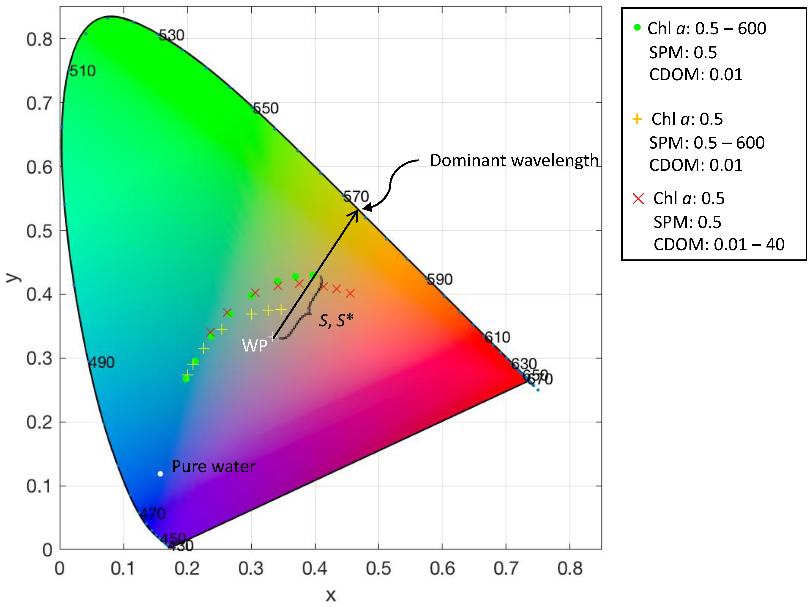
Figure 2.
Map of New Zealand showing the locations of 3820 lakes according to the Freshwater Ecosystems of New Zealand (FENZ) geodatabase [27]. The colour of the dots identifies the geomorphic lake type as per the labels of the pie chart. The pie chart shows the relative distribution of lake types.
Figure 2.
Map of New Zealand showing the locations of 3820 lakes according to the Freshwater Ecosystems of New Zealand (FENZ) geodatabase [27]. The colour of the dots identifies the geomorphic lake type as per the labels of the pie chart. The pie chart shows the relative distribution of lake types.

Figure 3.
Landsat 8 Operational Land Imager (OLI) images of three example lakes showing the 3-by-3 pixel area for which data was extracted. The outlines shown were taken from the FENZ geodatabase. North is up in all images. (a) Lake Rotokawau (volcanic lake) on 3 March 2017; (b) Lake Ngaroto (peat lake) on 2 March 2016; and, (c) Lake Wanaka (glacial lake) on 3 March 2017.
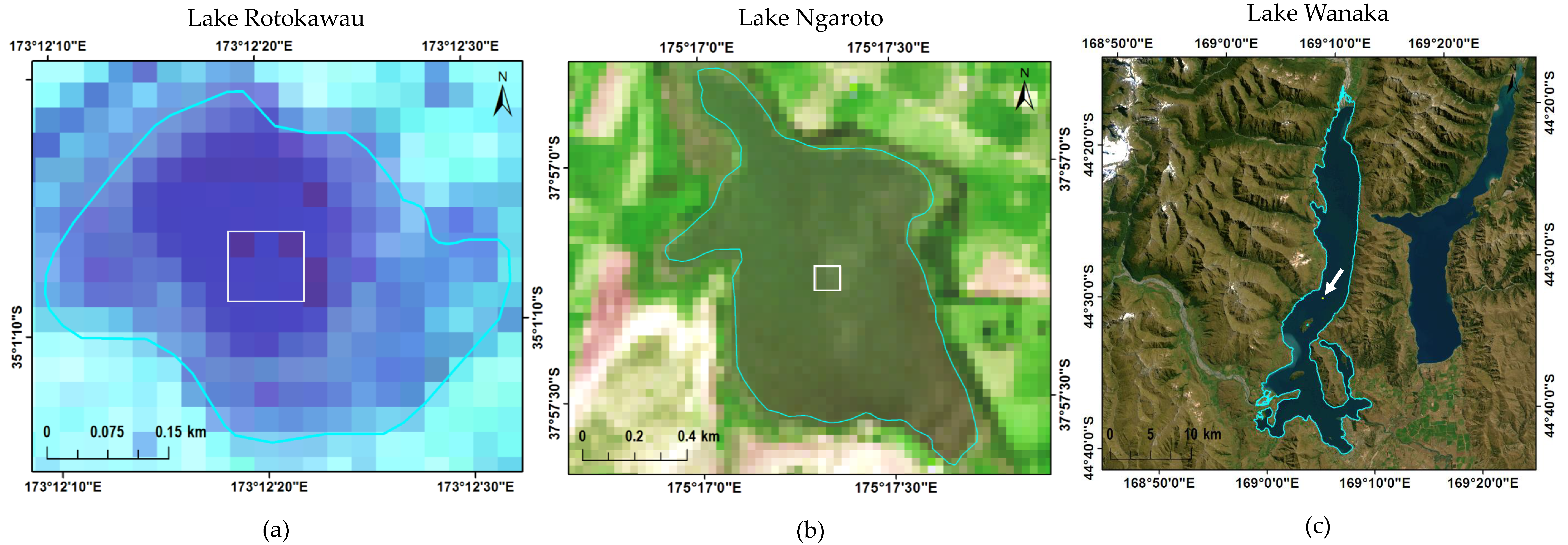
Figure 4.
(a) Deviation in degrees from the hyperspectral hue angle for the OLI instrument. The horizontal axis gives the hue angle based on the reconstructed spectra (scaled by 100 for practical reasons). The drawn line is the fifth order polynomial fit to the data. (b) Deviation in distance (S) of the hyperspectral distance from the universal white point.

Figure 5.
1486 lakes coloured by the average number of observations per year. The red rectangles delineate the geographic locations of the Landsat 8 OLI path/row scene boundaries of the descending (daytime) node in WRS-2 [49]. The boxes (a–d) show the locations of the closeup maps of Figures 9 and 12.

Figure 6.
(a) Frequency distribution of average number of observations per year for New Zealand lakes. (b) Box plot of the average number of observations of New Zealand lakes by month. On each box, the central mark indicates the median, and the bottom and top edges of the box indicate the 25th and 75th percentiles, respectively. The whiskers extend to the most extreme data points.

Figure 7.
Chromaticity diagram showing the water colour of 44,947 lake observations determined from Landsat 8 OLI data. The dashed lines from the white point (WP) to dominant wavelengths of 495 and 510 nm, respectively, indicate the nominal boundaries for colour classification into blue, green and red bins.

Figure 8.
(a) Frequency histogram of 44,947 observations of dominant wavelength. (b) Frequency distribution of the mean dominant wavelength of 1486 lakes.
Figure 8.
(a) Frequency histogram of 44,947 observations of dominant wavelength. (b) Frequency distribution of the mean dominant wavelength of 1486 lakes.
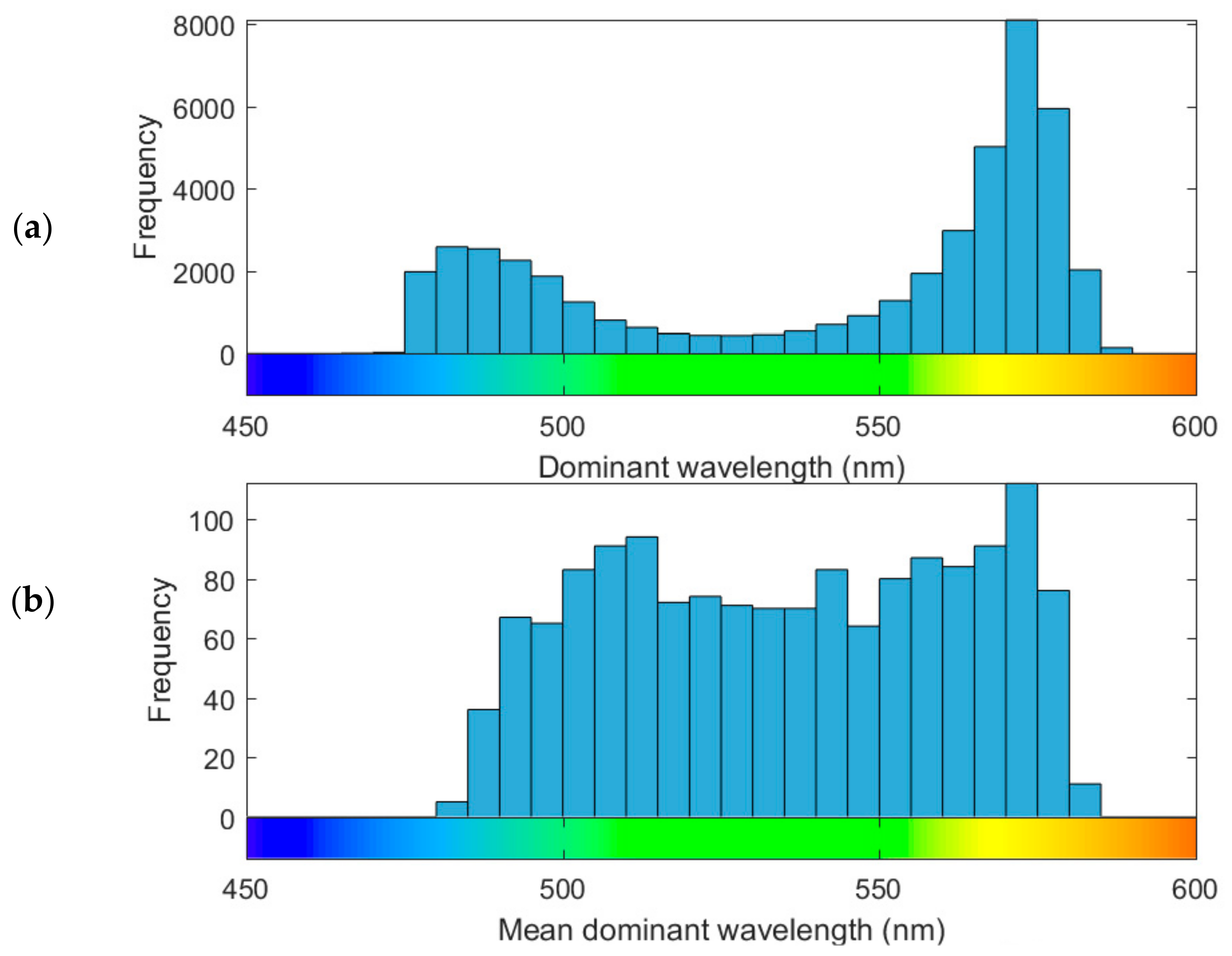
Figure 9.
Geographic distribution of lakes coloured by mean dominant wavelength in four areas. Placement of the areas shown in maps (a–d) are shown in Figure 5.
Figure 9.
Geographic distribution of lakes coloured by mean dominant wavelength in four areas. Placement of the areas shown in maps (a–d) are shown in Figure 5.
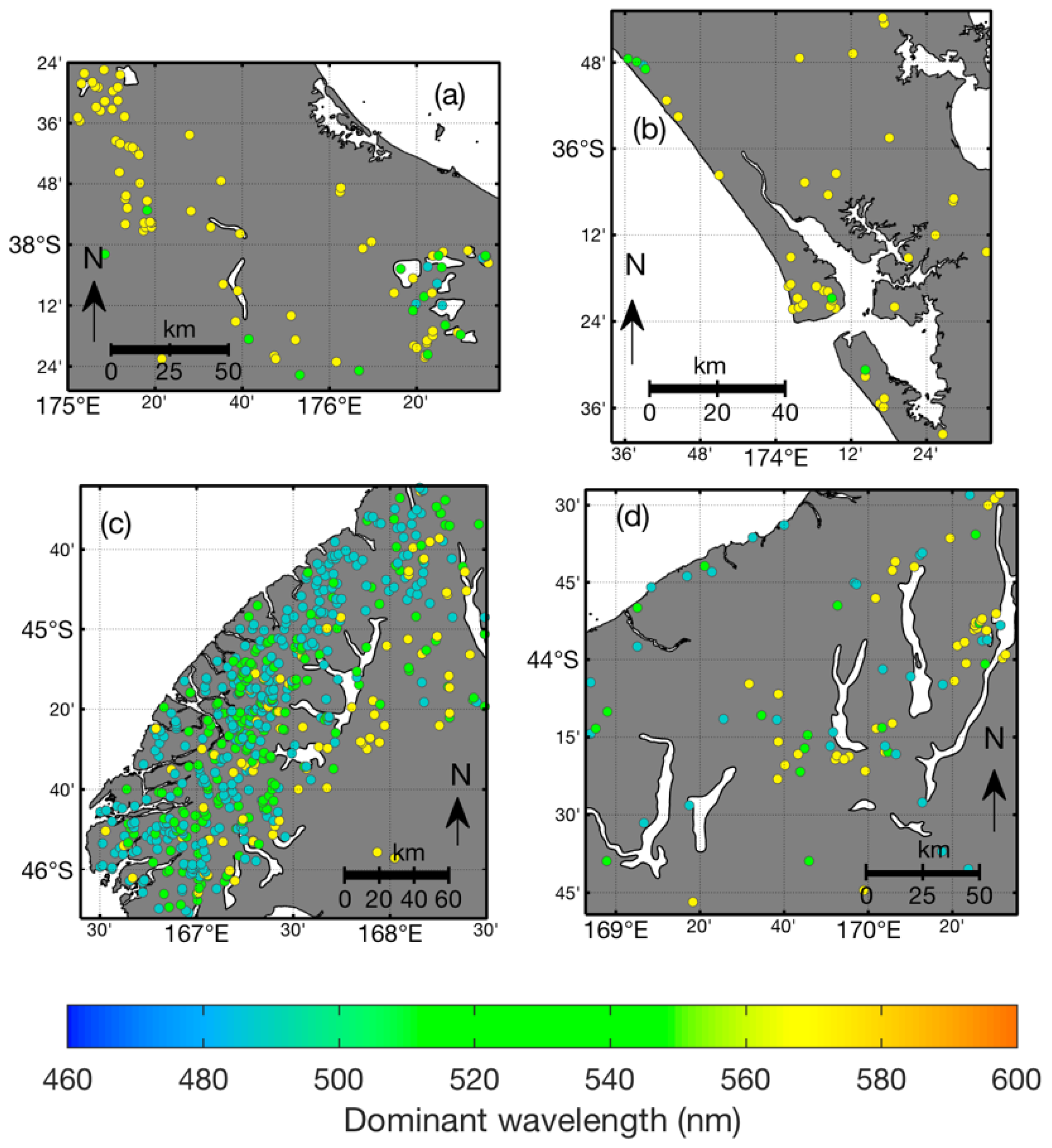
Figure 10.
Box plot of the distribution of dominant wavelength in 1486 lakes ordered by median dominant wavelength (black line). The bottom and top edges of each box indicate the 25th and 75th percentiles, respectively; blue lines extend to the most extreme data points not considered outliers, and outliers are shown as circles.
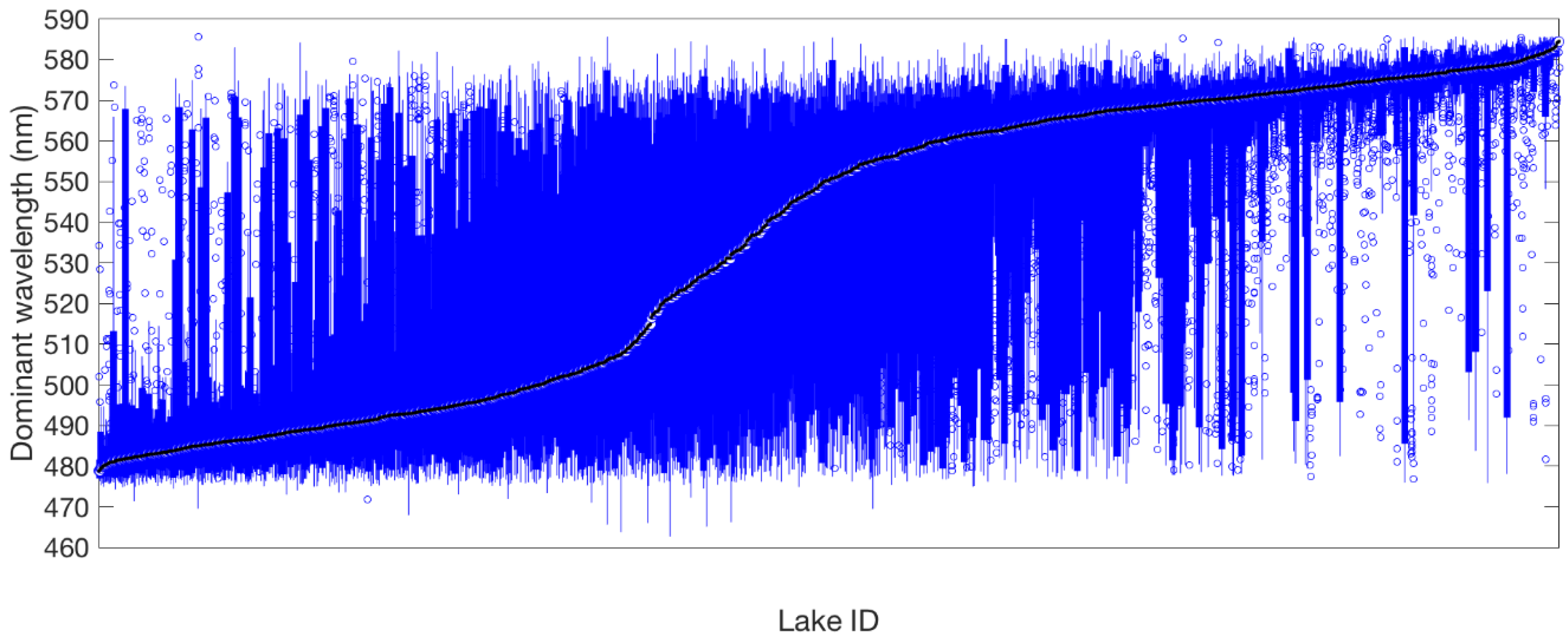
Figure 11.
Three example time series of (a) dominant wavelength and (b) purity and the location of each observation in a chromaticity diagram (c). The horizontal lines in (a) indicate the boundary wavelengths between blue and green colour bins (495 nm) and green and yellow colour bins (560 nm). Lake Pukaki (44.0542°S, 170.1685°E), Lake Rotomanuka (37.9257°S, 175.3152°E), and Lake Rotoiti (38.0358°S, 176.4174°E).
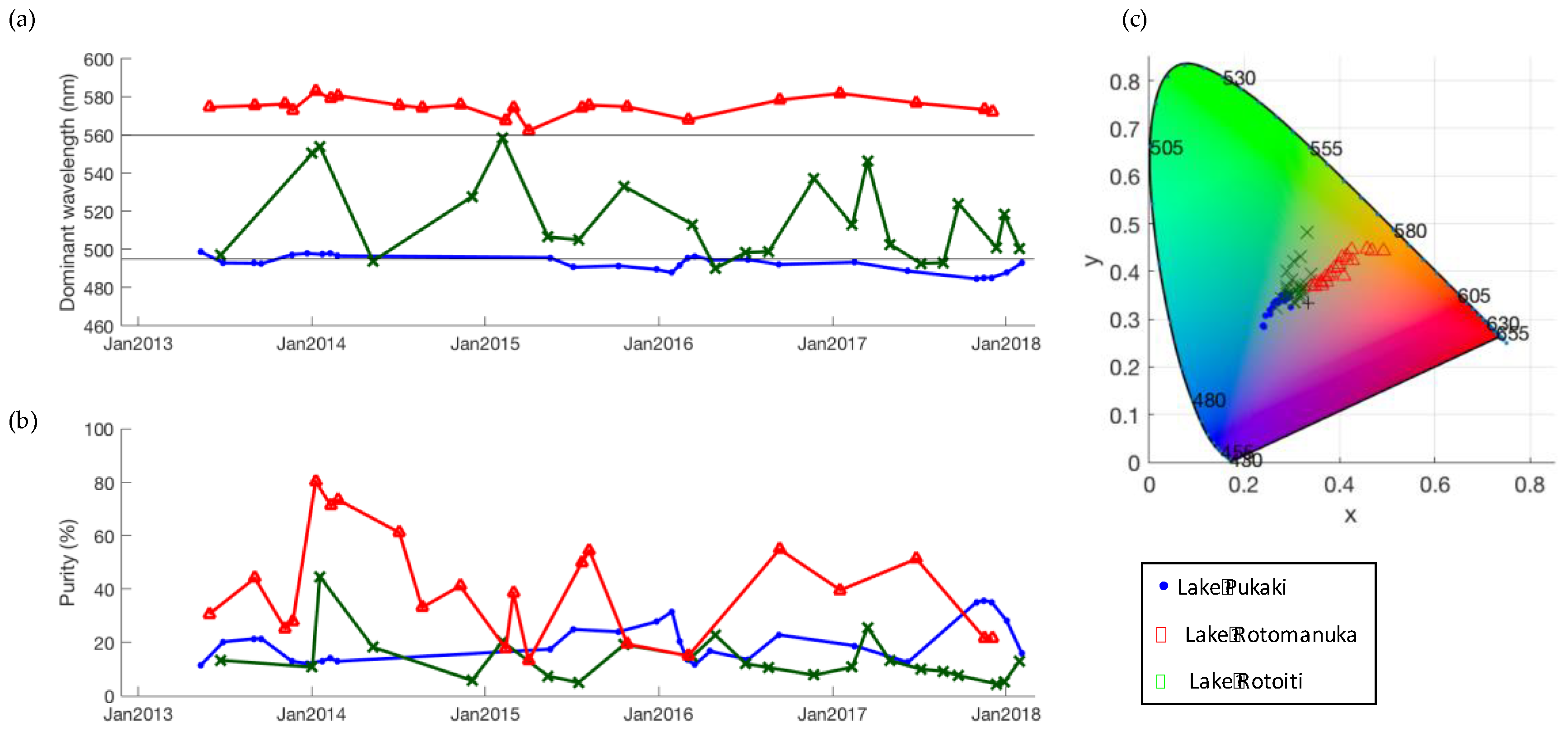
Figure 12.
Geographic distribution of lakes coloured by colour bins according to Table 1 in four areas. Placement of the areas shown in maps (a–d) are shown in Figure 5.

Figure 13.
Percentage distribution of lakes in colour bins according to Table 1 in elevation-depth classes [29]. Lowland and highland lakes are where the lake surface is below 300 m and above 300 m, respectively.

Figure 14.
Lake-mean dominant wavelength versus the percentage of land cover by high-producing exotic grassland (P) in the lake catchment (after logistic transformation). Dots are colour-coded according to colour bins (Table 1).
Figure 14.
Lake-mean dominant wavelength versus the percentage of land cover by high-producing exotic grassland (P) in the lake catchment (after logistic transformation). Dots are colour-coded according to colour bins (Table 1).


Table 1.
Colour bins and numbers of lakes in each bin according to their dominant wavelength distribution. Note that the percentages in the right-hand column add up to over 100% as some lakes fit into more than one category.
Table 1.
Colour bins and numbers of lakes in each bin according to their dominant wavelength distribution. Note that the percentages in the right-hand column add up to over 100% as some lakes fit into more than one category.
| Colour Bin 1 | Criterion | Number of Lakes 2 |
|---|---|---|
| Blue | ≥60% blue | 277 (18.6%) |
| Green | ≥60% green | 124 (8.3%) |
| Yellow | ≥60% yellow | 547 (36.8%) |
| Blue-green | ≥40% blue ≥20% green | 287 (19.3%) |
| Green-yellow | ≥40% yellow ≥20% green | 302 (20.3%) |
| Blue-yellow | ≥40% blue ≥40% yellow | 15 (1.0%) |
| Unassigned | None of the above | 195 (13.1%) |
1 Wavelength ranges (in nm) for colour bins are as follows; blue: λd < 495, green: 495 ≤ λd < 560, yellow: λd ≥ 560. 2 The percentage of lakes in a given colour bin is relative to the total number of lakes in this study (1486).
© 2018 by the authors. Licensee MDPI, Basel, Switzerland. This article is an open access article distributed under the terms and conditions of the Creative Commons Attribution (CC BY) license (http://creativecommons.org/licenses/by/4.0/).
Share and Cite
MDPI and ACS Style
Lehmann, M.K.; Nguyen, U.; Allan, M.; Van der Woerd, H.J. Colour Classification of 1486 Lakes across a Wide Range of Optical Water Types. Remote Sens. 2018, 10, 1273. https://doi.org/10.3390/rs10081273
AMA Style
Lehmann MK, Nguyen U, Allan M, Van der Woerd HJ. Colour Classification of 1486 Lakes across a Wide Range of Optical Water Types. Remote Sensing. 2018; 10(8):1273. https://doi.org/10.3390/rs10081273
Chicago/Turabian StyleLehmann, Moritz K., Uyen Nguyen, Mathew Allan, and Hendrik Jan Van der Woerd. 2018. "Colour Classification of 1486 Lakes across a Wide Range of Optical Water Types" Remote Sensing 10, no. 8: 1273. https://doi.org/10.3390/rs10081273
Note that from the first issue of 2016, this journal uses article numbers instead of page numbers. See further details here.