Unsupervised Deep Feature Learning for Remote Sensing Image Retrieval


1
Key Laboratory of Intelligent Perception and Image Understanding of Ministry of Education, International Research Center for Intelligent Perception and Computation, Joint International Research Laboratory of Intelligent Perception and Computation, School of Artificial Intelligence, Xidian University, Xi’an 710071, China
2
School of Computer Science and Engineering, Nanjing University of Science and Technology, Nanjing 210094, China
*
Author to whom correspondence should be addressed.
Remote Sens. 2018, 10(8), 1243; https://doi.org/10.3390/rs10081243
Submission received: 6 June 2018
/
Revised: 1 August 2018
/
Accepted: 2 August 2018
/
Published: 7 August 2018
(This article belongs to the Special Issue Image Retrieval in Remote Sensing)
Abstract
:Due to the specific characteristics and complicated contents of remote sensing (RS) images, remote sensing image retrieval (RSIR) is always an open and tough research topic in the RS community. There are two basic blocks in RSIR, including feature learning and similarity matching. In this paper, we focus on developing an effective feature learning method for RSIR. With the help of the deep learning technique, the proposed feature learning method is designed under the bag-of-words (BOW) paradigm. Thus, we name the obtained feature deep BOW (DBOW). The learning process consists of two parts, including image descriptor learning and feature construction. First, to explore the complex contents within the RS image, we extract the image descriptor in the image patch level rather than the whole image. In addition, instead of using the handcrafted feature to describe the patches, we propose the deep convolutional auto-encoder (DCAE) model to deeply learn the discriminative descriptor for the RS image. Second, the k-means algorithm is selected to generate the codebook using the obtained deep descriptors. Then, the final histogrammic DBOW features are acquired by counting the frequency of the single code word. When we get the DBOW features from the RS images, the similarities between RS images are measured using L1-norm distance. Then, the retrieval results can be acquired according to the similarity order. The encouraging experimental results counted on four public RS image archives demonstrate that our DBOW feature is effective for the RSIR task. Compared with the existing RS image features, our DBOW can achieve improved behavior on RSIR.
1. Introduction
With the imaging technique developed, the number of remote sensing (RS) images collected from earth observation (EO) satellites grows dramatically. Finding the specific region from a large number of RS images becomes the basic step for many RS applications [1]. Therefore, developing the rapid and accurate retrieval method to obtain the contents according to users’ demands has drawn increasing attention recently. In the past, the metadata within the EO products (e.g., acquisition time, longitude, latitude, etc.) was the key clue for content retrieval [2]. However, this text-based retrieval method is not able to deal with the increasingly complex tasks since the information within the metadata is limited. Thus, content-based image retrieval (CBIR) comes in the RS community. For a query image, CBIR utilizes a series of image processing techniques, such as feature extraction and similarity calculation, to retrieve the most similar target images from the image archive. Any approaches, focusing on organizing the image archive according to the images’ contents, can be regarded as the CBIR methods [3]. An ocean of successful CBIR methods was presented, such as [4,5,6], etc.
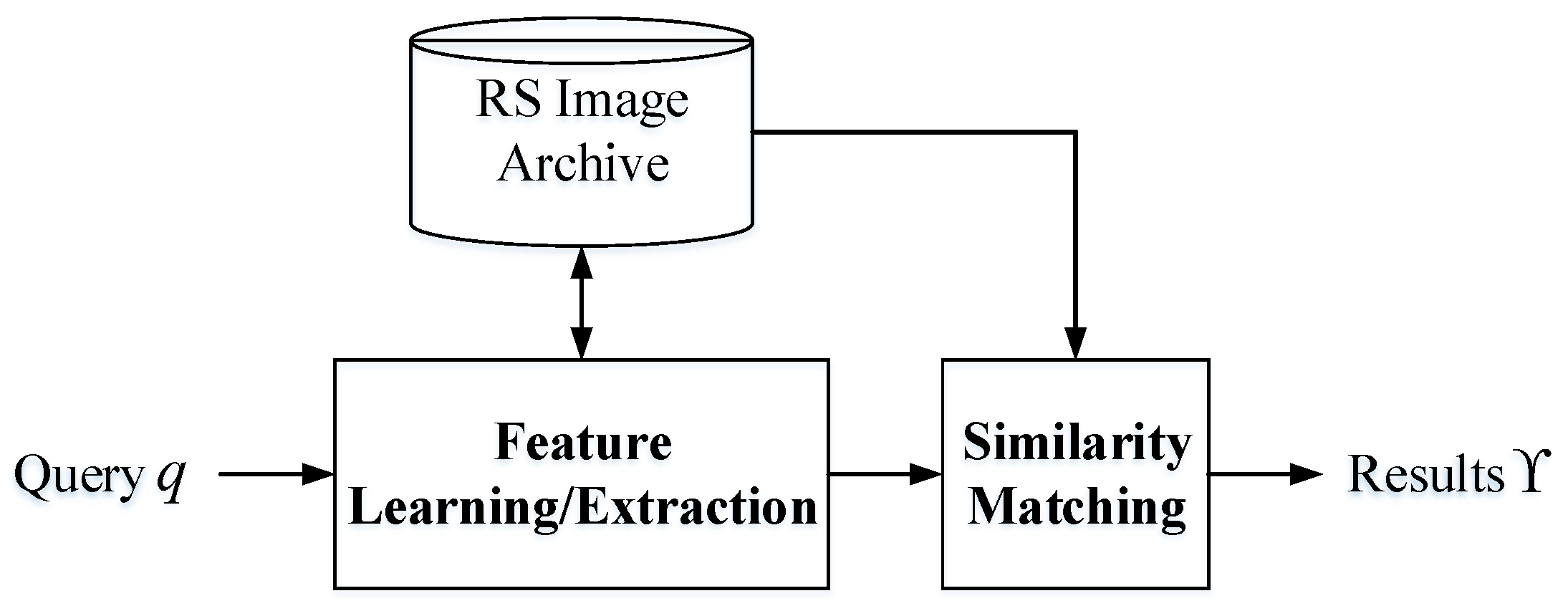
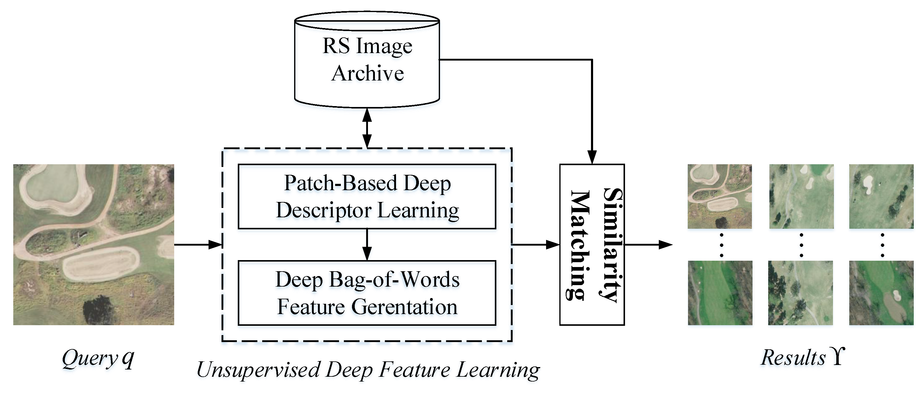
As an important application of CBIR, remote sensing image retrieval (RSIR) is developed based on the framework of CBIR. A basic flowchart of the RSIR method [7] is displayed in Figure 1, including two indispensable blocks. The first block is feature learning/extraction, which maps the query and target images into the feature space. The second block is similarity matching, which uses a proper measure to weigh the similarities between query and targets images. Then, the retrieval results of query q can be obtained by the similarity order. The main target of the feature learning/extraction block is obtaining the useful feature representation for RS images, while the primary goal of the similarity matching block is acquiring the resemblance between RS images efficiently. According to the basic framework, RSIR can be defined as follows. Assume that the RS image archive contains N images . For a query image q, its retrieval results can be described as
where indicates the distances between q and target images, which can be calculated in the feature space using a proper similarity metric, and denotes the ranking process.
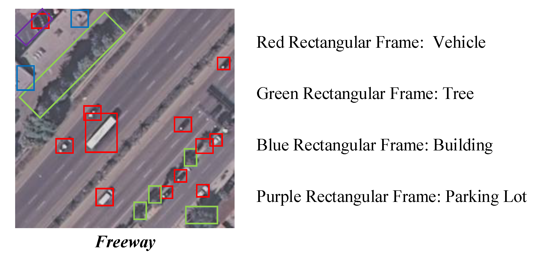
Although the basic RSIR system exhibited in Figure 1 is simple, the implementation is not as easy as as imaginary. For one RS scene, there are many specific characteristics that increase the difficulty of RSIR [8,9,10,11]. For example, the objects within one RS scene are diverse in type and huge in volume; the scales of the same objects may be different; and various thematic classes may be contained. There is an RS image shown in Figure 2. From the observation of Figure 2, we can find there are at least five kinds of objects, including “Freeway”, “Vehicle”, “Tree”, “Building”, and “Parking lot”. In addition, the scales of the same object are different (e.g., “Vehicle”). These special properties make the RSIR is an open and tough task.
As displayed in Figure 1, the first and crucial step of an RSIR method is the feature learning/extraction. The ideal RS image representation can not only capture the complex contents within the RS image, but also reflect the multi-scale characteristic of diverse objects [12]. Traditional features used for RS images are always handcrafted features, including the low-level and mid-level features. The common low-level features are the texture feature obtained from gray-level co-occurrence matrix (GLCM) [13], the energy of sub-band of discrete wavelet transform [14], the homogeneous texture feature obtained by Gabor filters [15], etc. The usual mid-level features are the Bag-of-Words (BOW) [16] feature and its extensions. Recently, with the development of the deep learning, especially the convolutional neural network (CNN) [17,18], the great changes have been placed in the RS image processing field. More and more successful applications [19,20,21,22] prove that the features learned by CNNs are more effective for describing the RS images. These kinds of features are named high-level features or deep features.
Although the aforementioned features provide the positive contributions to RSIR, their drawbacks are also distinct. For low-level and mid-level features, their RSIR performance is stable but satisfactory enough [1]. The deep feature achieves cracking behavior in RSIR; nevertheless, the learning process is expensive since the most of the CNNs are supervised models, which need a tremendous amount of labels. Therefore, it is necessary to develop an effective and cheap deep feature learning/extraction method for RSIR.
In this paper, we present a new deep feature learning method for RSIR. Different from most of the existing CNN based methods, our deep feature learning method is an unsupervised model. It is developed in the BOW framework, so we name it deep bag of words (DBOW) in this paper. Like the BOW feature, we can obtain the DBOW feature by the following two steps: (i) learning the deep descriptors, and (ii) encoding the DBOW feature. For step (i), to decrease the difficulty of deep descriptor learning, we divide an RS image into image patches. On the one hand, the sub-sampled patches are less complex and more compact for exploring the diverse contents of RS image. On the other hand, the multi-scale property can be fully captured though adjusting the size of patches, which is an ordinary process. Moreover, we propose the deep convolutional auto-encoder (DCAE) model to obtain the discriminative features from those patches, which are regarded as the deep descriptors of the RS image. For step (ii), the k-means algorithm is used to cluster all of the deep descriptors to get the codebook. Then, the DBOW feature corresponding to an RS image can be acquired by counting the frequency of the single codewords. Finally, the retrieval results are obtained according to the distances between DBOW features.
The main contributions of our work can be summarized as follows:
- Taking the properties of complex contents and multiple semantic classes into account, we use image patches rather than the whole RS image to learn the descriptors. This is beneficial to capture the information of diverse objects.
- Considering the multi-scale characteristic, we choose two patch generation schemes to generate two kinds of patches with different scales. In addition, the different kinds of patches can capture the complex contents within the RS image in a complementary manner.
- To deeply mine the inner information of image patches and obtain the effective representations, rather than the handcrafted feature, we develop an unsupervised deep learning model to learn the discriminative descriptors.
- Experiments are conducted on different RS image data sets, which cover different resolutions and different types of RS images. The encouraging results prove that the deep feature obtained by our method is effective for RSIR.
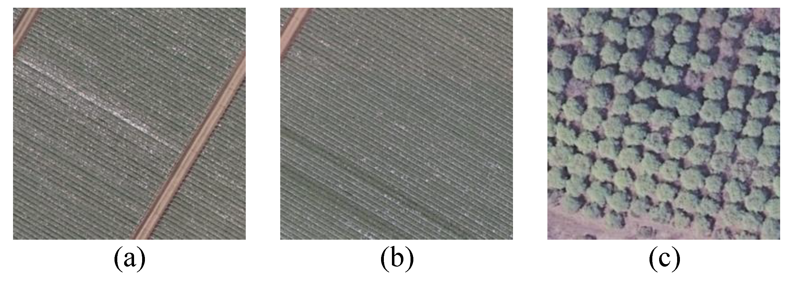
Before describing our RSIR method, there are two points we want to explain. The first is the difference between the RS image classification and RSIR, which are two hot research topics in the RS community. Image classification aims at grouping the images according to some common characters, while RSIR focuses on finding the similar images from the archive in accordance with the contents. We take three RS images exhibited in Figure 3 above as an example. All of them are labeled “Agricultural” in the UCMerced archive [23,24]. The goal of image classification is developing a classifier to categorize them into same group. Nevertheless, the target of RSIR is finding the similar ones. In other words, Figure 3b, rather than Figure 3c, should be ranked higher if Figure 3a is the query. In short, the biggest difference between image classification and image retrieval is that the images within the same class may not similar.
The second one is the difference between our retrieval method and another RSIR approach proposed in the literature [25], which was developed on the basis of the BOW based CNN model. Although both of us utilize the BOW and the deep neural network paradigm to complete RSIR, there are still many differences between two methods.
- First, the retrieval scenario is different. The method proposed in [25] aims at text-based image retrieval. The original query is the text (e.g., “Daisy Flower”). In addition, to obtain the accurate retrieval results, the authors expand the input using the click through data. The final query is the combination of the text and clicked images. Our method focuses on image-based retrieval, i.e., the input is only an image without any text information.
- Second, the units for BOW construction is different. The basic units for constructing the BOW feature in [25] are the text words. For example, the BOW feature of a “puppy dog” image is {“small dog”, “white dog”, “dog chihuahua”}. The values of different elements can be represented by the inverse document frequency (IDF) score [26]. The basic units for constructing the BOW feature in our method are visual words, i.e., image patches. Since we use a deep neural network to learn the representation of patches, we name the final BOW feature DBOW.
- Third, the framework is different. For the method in [25], the BOW features are used to train the CNN model. As mentioned above, when user inputs a query text, a set of images can be obtained according to the click through data. The function of the CNN model is ranking these images based on their similarity relationships, which are decided by BOW and high-level visual features simultaneously. For our method, the CNN model is used to generate the DBOW features. We use the DCAE model to learn the latent features from the image patches. Then, the learned deep features are integrated to construct the DBOW features. The retrieval results of a query image are decided by a proper distance metric (e.g., L1-norm) in the feature space.
Apart from the differences discussed above, there is another important point we want to touch. This is that the deep neural network in [25] should be trained in the supervised manner, while our DCAE model can be trained in the unsupervised manner.
The rest of this paper is organized as follows. The published literature related RSIR are discussed in Section 2. Section 3 presents the proposed deep feature learning method, including the preliminaries, deep descriptor learning, and DBOW feature generation. The experimental results counted on different RS data sets are displayed and discussed in Section 4. Section 5 provides the conclusions.
2. Related Work
This section briefly reviews the published literature related to RSIR. As mentioned in Section 1, there are two key techniques in a basic RSIR system. Thus, we broadly classify the existing RSIR methods into two groups, i.e., feature representation based RSIR and similarity matching based RSIR.
2.1. Feature Representation Based RSIR
The methods categorized in this group emphasize the contribution of image feature to RSIR. As early as 1998, two RSIR methods based on feature representation were proposed [27,28]. Two models, Bayesian and Gibbs–Markov random field (GMRF), were selected to capture the spatial information from RS images, respectively. The feature extraction was transformed into the parameter estimation issue in these two methods. The retrieval results were obtained under the Bayesian paradigm. Then, Datcu et al. [2] introduced another information based RSIR method. The retrieval results were obtained by the dyadic k-means algorithm [29] using the feature extracted by a hierarchical Bayesian model. A comprehensive RSIR system named Geospatial Information Retrieval and Indexing System (GeoIRIS) was proposed in the literature [30]. GeoIRIS integrated six modules to accomplish diverse complex tasks related to RSIR. Among these modules, the fundamental and crucial module of GeoIRIS was feature extraction. To describe the RS image accurately, diverse features were extracted, including the spectral features, texture features, linear features, object-based features, etc. Yang and Newsam [23] tried to deal with the RSIR task using the local invariant features. The scale invariant feature transform (SIFT) descriptor [31,32] based BOW features were extracted from the RS images, and the retrieval results were obtained by the L1-norm distance. Based on the Fourier power spectrum of an image’s quasi-flat zones representation, Aptoula proposed the global morphological texture descriptors for RSIR in the literature [33]. The behavior of new descriptors was verified using the published image archive. To explore the local textural and structural information of RS images, the local extrema descriptor was introduced in [34], in which the radiometric, geometric and gradient properties of RS images can be captured. To enhance the retrieval efficiency, Demir and Bruzzone [12] introduced the hashing code into RSIR. Compared with the dense features mentioned before, the hashing feature accelerated the speed of retrieval obviously.
The features used in the RSIR methods mentioned above are all handcrafted. Although the results are positive, their contributions to the RSIR are limited due to the complexity of RS images. Recently, due to the strong representation capacity, the deep features learned by the deep neural network model made the cracking contributions to RSIR. Zhou et al. [35] utilized the auto-encoder to learn the sparse features from RS images, and the retrieval results were obtained by L1/L2 norm distance. Li et al. [36] combined the deep features and low-level handcrafted features together to represent RS images. The retrieval results were obtained by the collaborative affinity metric fusion. Zhou et al. [37] presented a low dimensional CNN model to learn the representative features from the RS images for RSIR. Since the novel framework of the introduced CNN model, the dimension of the obtained features was lower than that of the traditional CNN. A deep hashing neural network was proposed to learn the hashing code of RS images for large-scale RSIR [38]. The dual CNNs framework was developed to learn the deep features and deep hashing code simultaneously. In addition, to train the proposed network with the limited labeled RS images, the transfer learning theory was introduced.
2.2. Similarity Matching Based RSIR
The RSIR methods within this group aim at improving the RSIS behavior through the dedicated similarity measures. Datta et al. [39] presented an RS image information mining system based on the image classification and region-based similarity measure, i.e., integrated region matching (IRM) similarity measure. To weight the similarities between RS images properly, IRM segmented the image into several regions first, and then calculated the distances using discrete feature sets corresponding to different regions. An improved IRM (IIRM) measure was introduced in [40] for dealing with synthetic aperture radar (SAR) image retrieval. Two kinds of segmented regions were obtained using different features, and the similarity between two SAR images was computed by the weighted linear summation of two IRM distances. To deal with the blurry boundaries and segmented uncertainty of segmented regions, the region-based fuzzy matching (RFM) measure was proposed in [41] for SAR image content retrieval. The fuzzy features were utilized to represent the gradual transition between adjacent regions. The resemblance between two SAR images was calculated using the fuzzy theory.
Besides the RSIR methods displayed above, which directly design the similarity measure according to the RS images’ properties, there are still many successful tool-based works have been proposed. The entropy-balanced bitmap (EBB) tree was used in [42] to explore the similarities between RS images using the shape features. A three-layer graph-based framework [43] was proposed to fuse the contributions of diverse low-level features and query expansions for deciding the resemblance between RS images. Tang and Jiao [44] introduced a fusion similarity measure and graph-based reranking method to improve the performance of SAR image retrieval. The authors adopted several SAR-oriented features to construct the modal-image matrix for the calculation of fusion similarities, and then the preliminary SAR image retrieval results were refined under the graph theory. A two-step reranking method was presented in [45]. Based on the initial retrieval results, the active learning based edit scheme and multiple graph based reranking approach were integrated to re-define the similarities between RS images for enhancing the RSIR’s behavior.
3. Methodology
Similar with the basic RSIR pipeline, the framework of RSIR based on the proposed feature learning method is shown in Figure 4. When a user inputs the query image q, its DBOW feature is learned by our feature learning method. Then, the similarities between the query and target RS images are calculated in the feature space to obtain the retrieval results . To ensure the obtained feature can capture the complex contents of RS image, our feature learning algorithm is divided into two parts, including “Patch-Based Deep Descriptor Learning” and “Deep Bag-of-Words Generation”. The first part aims at finding the effective image descriptors with the help of deep learning, while the second part focuses on integrating all deep descriptors together to generate the final DBOW.
3.1. Preliminaries
To describe our feature learning method more clearly, we first introduce some preliminaries in this part.
3.1.1. Convolutional Auto-Encoder
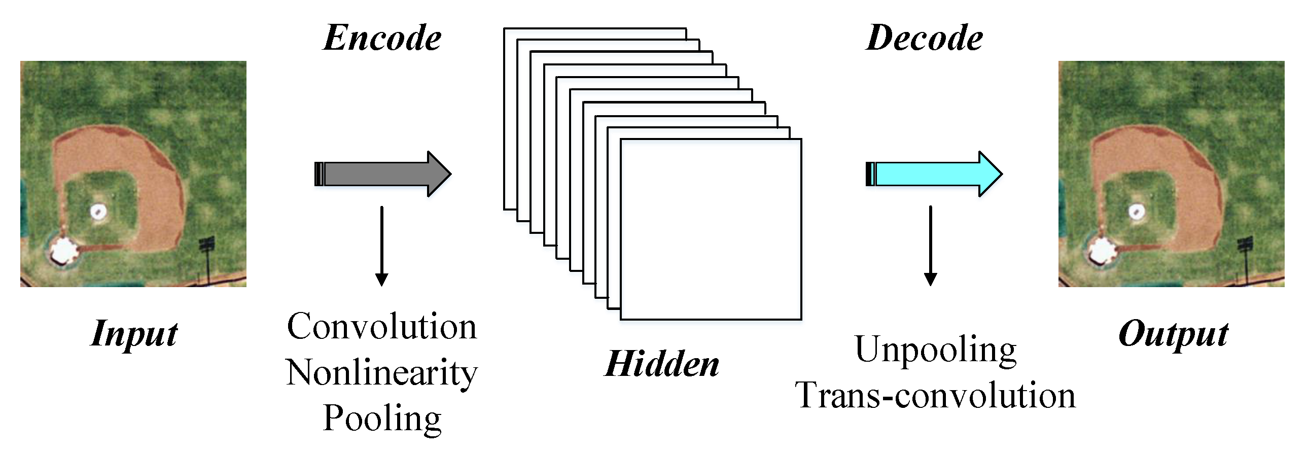
Convolutional Auto-Encoder (CAE) [46] is a popular and effective unsupervised feature learning technology, which is developed based on Auto-Encoder (AE). Similar to AE, CAE is a hierarchical feature extractor, aiming at discovering the inner information of images. Unlike AE, due to the utilization of the two-dimensional convolution, CAE can preserve the images’ structure (e.g., neighborhood relationship, spatial locality, etc.) during the feature learning, which is beneficial to obtain the more discriminative features. A CAE model usually consists of an input layer, a hidden layer, and an output layer [9]. The transformation from the input data to the hidden layer is named “encode”, while the procedure from the hidden layer to the output data is recoded “decode”. The target of encode is mining the inner information of the input data, and the goal of decode is re-constructing the input data. The framework of common CAE is exhibited in Figure 5.
The basic operations within the encode section consist of convolution, nonlinearity and pooling, which aim at extracting the detail information, increasing the nonlinear capacity, and avoiding the overfitting, respectively [46]. Assume that we use I to represent the input image, and I is a mono-channel image. Thus, the encode process of CAE can be formulated as
where indicates the k-th feature map in the hidden layer, means the network parameters related to the k-th feature map, ⊗ is the convolution, and denotes the activation function. The modules within the decode stage contain unpooling and trans-convolution, which focus on up-sampling and reconstruction separately. We can formulate the decode process as
where means the group of feature maps within the hidden layer, is the transposition of , is the bias, and denotes the re-constructed data. To update the parameters of CAE, the mean-squared error loss function is always selected:
where indicates the set of train samples consisted of N images , means the set of re-constructed samples corresponding to the train sample set, and denotes the parameters of CAE.
3.1.2. Bag-of-Words Feature
BOW feature [47] is a popular histogrammic feature representation in the RS image processing community. Its usefulness is proved by many successful applications [23,48]. The usual steps for generating the BOW feature are: (i) collect the key points of the images; and (ii) transform the key points into the histogrammic features. For step (i), the SIFT descriptor is often used to find the key points. For step (ii), researchers always select the k-means algorithm to construct a codebook, and then the BOW features can be obtained by counting the distances between key points and codewords. The performance of the BOW feature is impacted by several factors, such as the type of key points, the codebook size, etc. Among these factors, the key points extraction is the foundation, which restricts the behavior of the BOW feature directly.
Although the normal BOW feature has been achieved successes in different RS applications, its performance is always limited since the complex contents of RS images. In this paper, to capture the diverse information of RS images, the DCAE is used to learn the deep descriptors for RS images. Then, the more effective DBOW features can be generated using the learned descriptors.
3.2. Patch Based Deep Descriptor Learning
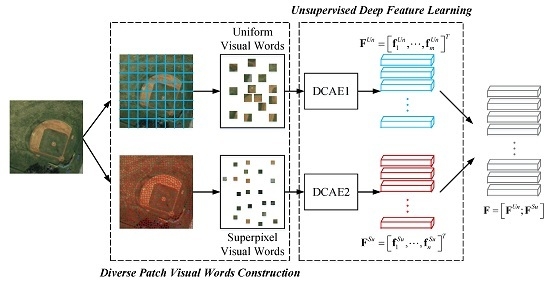
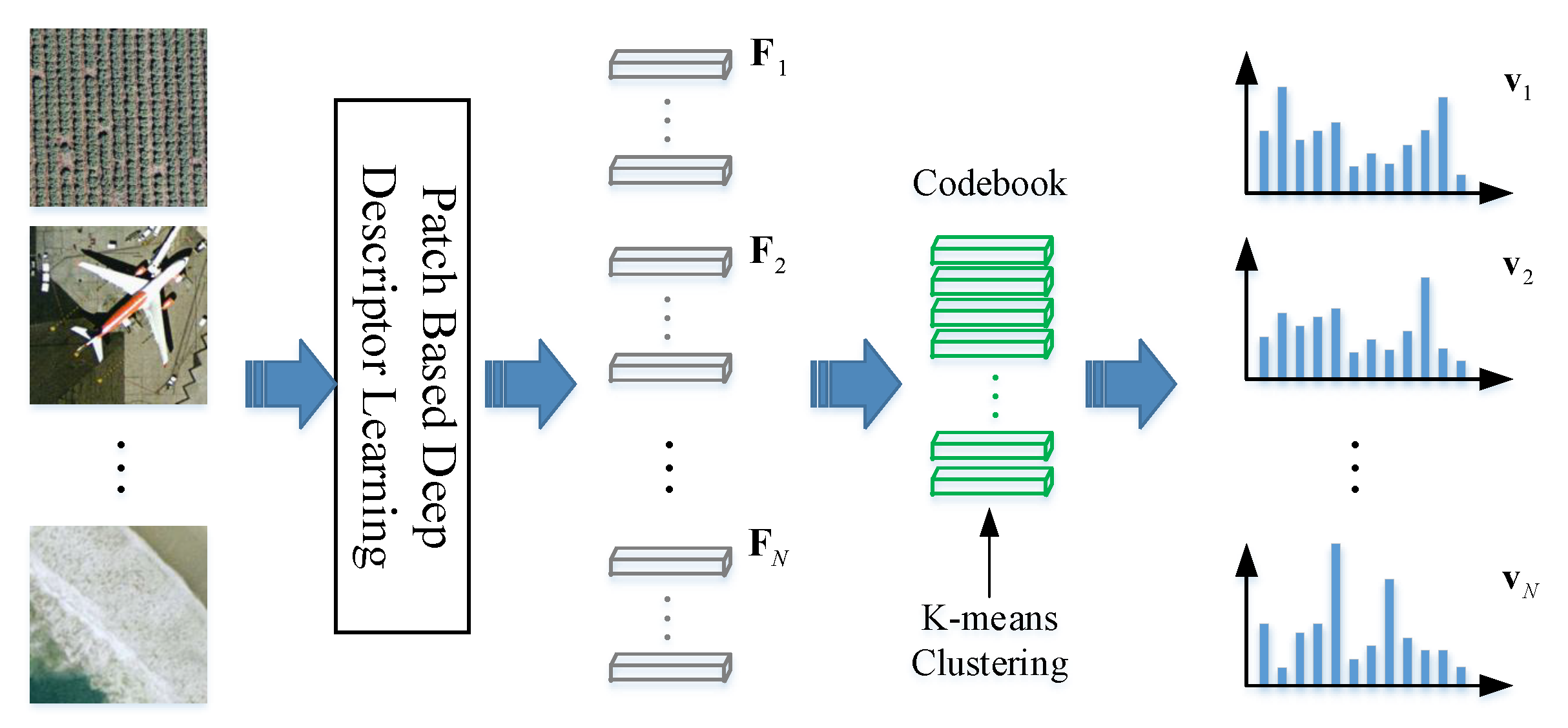
Due to the specific properties of RS image (e.g., contents are diverse in type and large in volume, the scale of different objects is different, etc.), we propose a patch based deep descriptor learning method to extract the effective image descriptors for DBOW. The framework of the proposed descriptor learning method is shown in Figure 6. It consists of two parts, i.e., diverse visual words construction and unsupervised deep feature learning. The visual words of an RS image are generated by different region sampling schemes, in which both the diversity of objects and the multi-scale characteristic are taken into account. The unsupervised feature learning is accomplished by DCAE models, which are strong enough to learn the effective latent features from the patches. Finally, to grasp the information from the global aspect, we stack the learned deep features corresponding to different patches together to construct the deep descriptor.
3.2.1. Diverse Patch Visual Words Construction
To mine the RS image’s information comprehensively, we use different region sampling schemes to generate diverse types of visual words.
First, the uniform grid-sampling scheme [49] is introduced. The scheme divides the RS image into a number of regular rectangle regions with the same size. Then, the RS image can be represented by a set uniform image patches. We record these patches uniform visual words here for short. The size and spacing of the grid influence the uniform visual words directly in general. In this paper, we divide the RS image into a series of non-overlapped patches, so that only the size of the grid should be considered in the following experiments.
Second, the superpixel technique is selected to generate another set of visual words. We name them superpixel visual words in this paper. A superpixel is an image over-segmented region obtained by some constraints [50], such as pixel value, location, etc. The desirable superpixels can adhere well to image boundaries, and group similar pixels together accurately. These advantages are beneficial for exploring the complicated objects within the RS images. Thus, choosing a good superpixel algorithm is important to superpixel visual words construction.
In this paper, the simple non-iterative clustering (SNIC) [51] algorithm is chosen to generate the superpixels. The SNIC algorithm begins with the superpixels’ centroids initialization, which is completed by sampling the pixels in the image plane. Then, the priority queue and online update scheme are utilized to adjust the initial superpixels according to the distances between those superpixels and their 4- or 8-connected pixels. To accurately weigh the distances between pixels and centroids, each pixel is described using a 5-dimensional vector , where indicates the pixel’s location, and denotes the pixel value in CIELAB color space. The formulation of distance between pixels is
where s and are the parameters for normalizing the spatial and color distances. The parameter s can be decided by the expected number of superpixels K according to the formulation , where indicates the number of pixels in an image. The parameter should be provided by users. SNIC is an improved version of the successful simple linear iterative clustering (SLIC) algorithm [52]. Compared with SLIC, SNIC can achieve higher performance with less time. More details can found in the original literature [51].
The shape of superpixels is irregular, and the size of superpixels is not strictly uniform. To use DCAE to learn their latent features, we should unify the shape and size of those superpixels. Here, a simple scheme is used to normalize the shape and size of superpixels. First, we record the locations (image plane) of all pixels within a superpixel. Then, the maxima and minima of the x-axis and y-axis are selected, which are recorded , , , and . Next, a rectangle region can be fixed, and the coordinates of the four vertices are , , , and . Finally, all of the rectangle regions are re-sized to the same size. The set of normalized superpixels is the superpixel visual words.
3.2.2. Unsupervised Deep Feature Learning
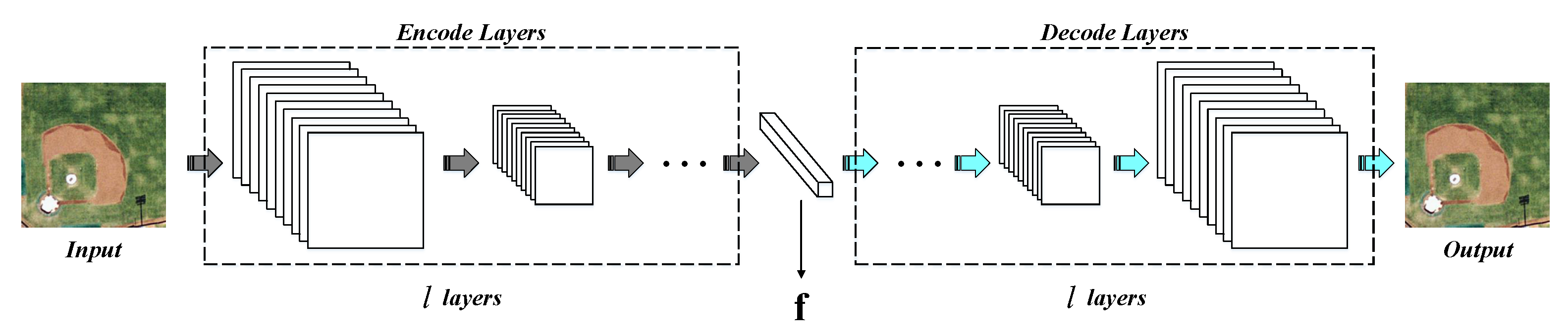
When we obtain the visual words of an image, the next step is learning their latent features using the CAE. To mine the deep latent feature from the visual patches, we expand the single CAE to the DCAE in this work. The framework of the utilized DCAE is shown in Figure 7. Note that we stipulate that the size of different kinds of visual words is the same. In other words, the superpixels should be normalized to the size of , which keeps pace with the uniform visual words.
The DCAE model transforms the input image I into a latent feature vector through l encode layers. Symmetrically, there are also l decode layers to re-construct the input image. Like CAE, we also use the mean-squared error loss function here to update the weights of our DCAE. The number of encode/decode layers l could be valued according to the size of input data. Here, to speed up the DCAE training and ensure the convergence of network, we initialize the parameters of DCAE in greedy, layer-wise fashion [9,53]. In other words, l CAEs are pre-trained for the initialized parameters.
As shown in Figure 6, there are two sets of visual words for an RS image I. Thus, we adopt two DCAE models to extract their latent features, respectively. Assume that there are m patches in the uniform visual words, and n patches in the superpixel visual words. Through two different DCAEs, we can obtain the latent features and , where corresponds to the i-th patch within the uniform visual words and relates to the j-th patch within the superpixel visual words. After that, two sets of latent features will be stacked together for constructing the deep descriptor for I.
3.3. Deep Bag-of-Words Generation
Suppose there are N RS images in the archive. After the deep descriptor learning procedure discussed in Section 3.2, we can obtain N deep descriptors . Since the number of patches of different RS images is different, the size of the deep descriptors is not uniform. It is hard to calculate the similarities between RS images using their deep descriptors directly. Consequently, we imitate the BOW feature to transform deep descriptors into the histogrammic feature, and name the final representation DBOW. The pipeline of DBOW generation is exhibited in Figure 8.
Like BOW feature, the codebook should be constructed first. Here, we integrate all of the deep descriptors together and use a k-means algorithm to group them into k clusters. The centers of different clusters are regarded as the codebook. Then, the deep descriptors learned from each RS images are mapped on the codebook and quantized by assigning the label of the nearest codeword. Finally, the DBOW feature of the RS image can be represented by the histogram of the codewords.
3.4. RSIR Formulation
When we get the DBOW features from the RS images, the retrieval results can be obtained according to the proper histogram-based distance metrics, such as L1-norm distance, L2-norm distance, cosine distance, etc. In more detail, for the query q and target RS images , the retrieval process can be formulated as , where indicates the distances between q and target images, which can be calculated using the DBOW features and . For example, suppose we select L1-norm distance to measure the similarities between images, the definition of is , where d indicates the dimension of DBOW features, means the j-dimensional element of , and illustrates the j-dimensional element of .
4. Experiment and Discussion
All of the experiments are completed using an HP Z840 workstation (Hewlett: Packard, Palo Alto, CA, USA) with GeForce GTX Titan X GPU (NVIDIA: Santa Clara, CA, USA), Inter Xeon E5-2630 CPU and 64G RAM (Intel: Santa Clara, CA, USA).
4.1. Experiment Settings
4.1.1. Test Dataset Introduction
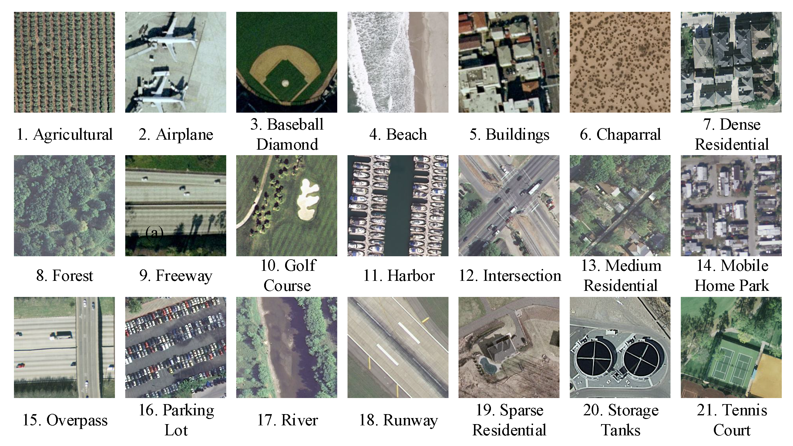
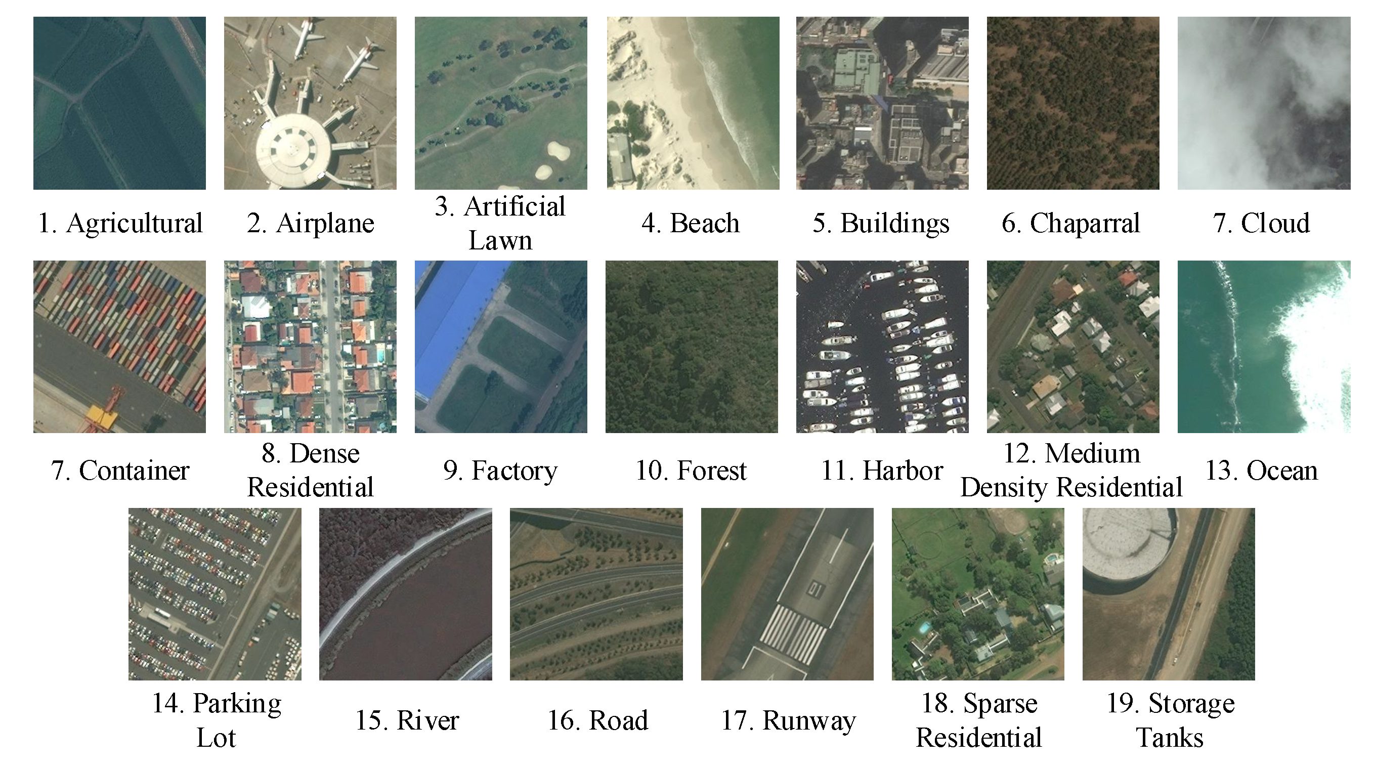
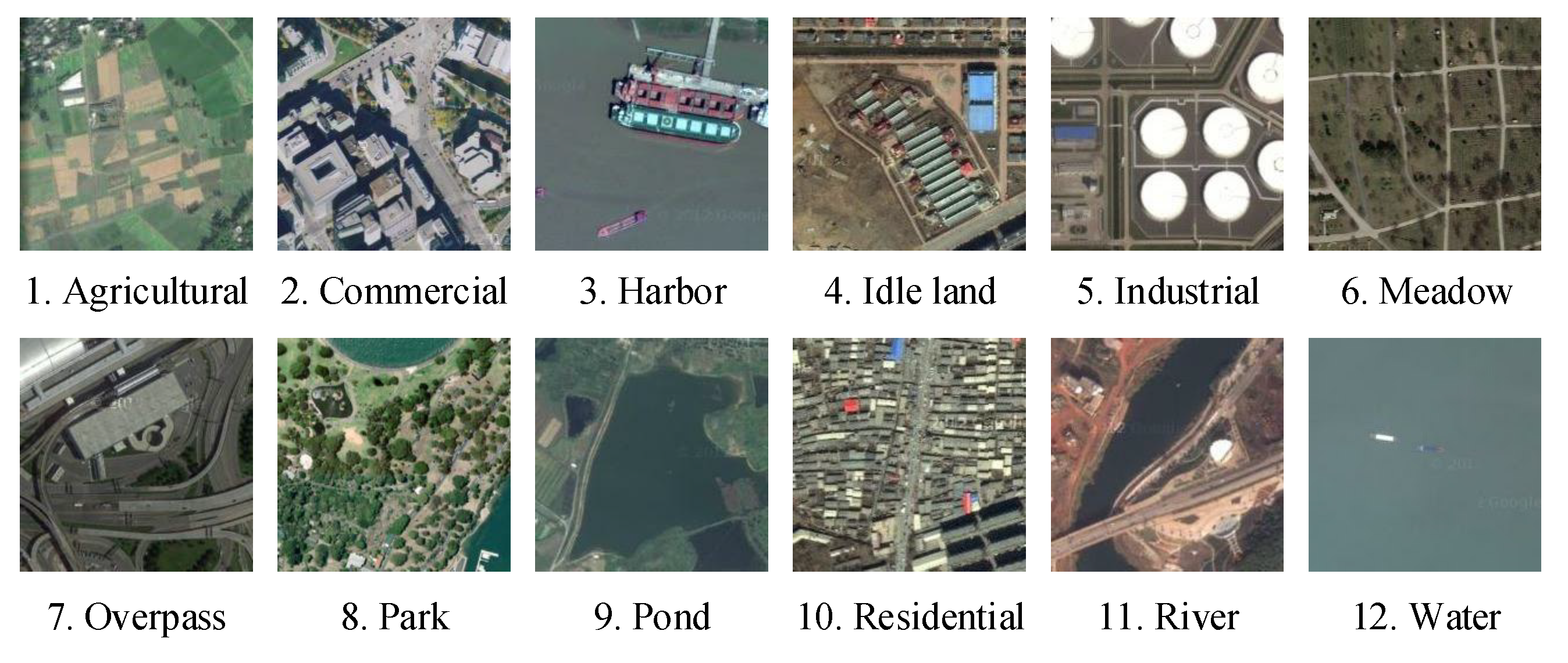
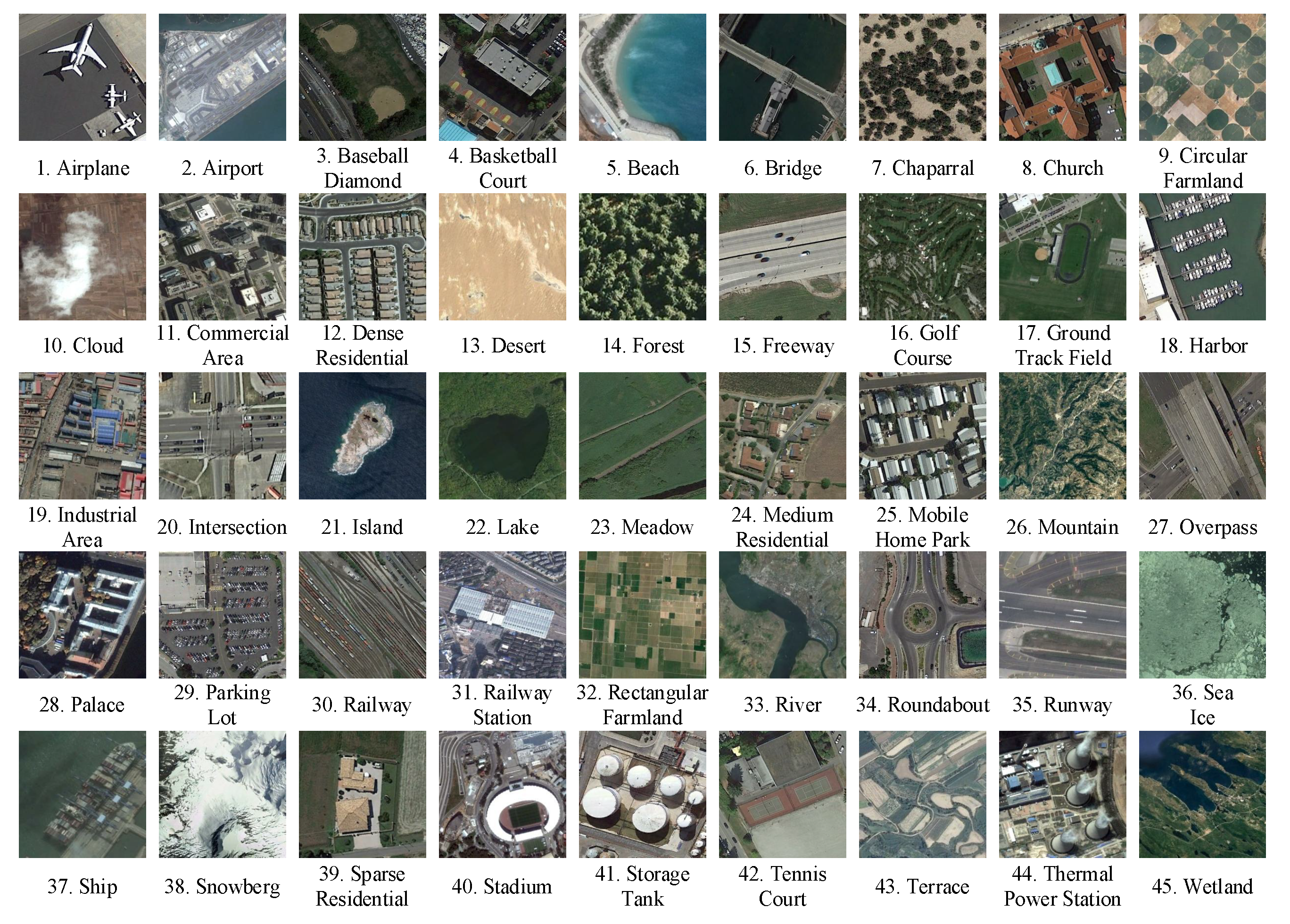
To comprehensively verify the effectiveness of our method, we apply it on four published datasets. The first data set is the UCMerced archive [23,24] (http://vision.ucmerced.edu/datasets/landuse.html). There are 21 land-use/land-cover (LULC) categories in this data set, and the number of high-resolution aerial images within each category is 100. The pixel resolution of these images is 0.3 m, while the size of them is . We name the UCMerced archive ImgDB1 in this paper for short, and some examples are exhibited in Figure 9. The second one is a satellite optical RS image data set [45] (https://sites.google.com/site/xutanghomepage/downloads). There are a total of 3000 RS images with a ground sample distance (GSD) of 0.5 m in this archive. These RS images are manually labeled into 20 land-cover categories, and the number of images within each category is 150. The size of these RS images is also . We record this archive ImgDB2 in this paper for convenience, and some examples are displayed in Figure 10. The third one for testing our method is a 12-class Google image data set [48,54,55] (http://www.lmars.whu.edu.cn/prof_web/zhongyanfei/e-code.html). For each land-use category, there are 200 RS images with the spatial resolution of 2 m. The size of images within this archive is . We record Google image data set ImgDB3 here for short, and some examples from different categories are shown in Figure 11. The last one is the NWPU-RESISC45 (http://www.escience.cn/people/JunweiHan/NWPU-RESISC45.html) data set, which was proposed in [56]. The NWPU-RESISC45 data set is a large-scale RS image archive, which consists of 31,500 images and 45 semantic classes. All of the images are collected from Google Earth, covering more than 100 countries. The spatial resolution of those images varies from 30 to 0.2 m, and the size of each image is . We record NWPU-RESISC45 ImgDB4 here for conveniens, and some examples are displayed in Figure 12.
4.1.2. Experimental Settings
As displayed in Figure 4, the pipeline of the RSIR method in this paper consists of feature learning and similarity matching. For feature learning, the proposed DBOW features are learned from each RS image. Then, the similarity matching is completed using the simple distance metric.
To accomplish our unsupervised feature learning method for RSIR, there are some parameters that should be set in advance. In the visual words construction stage, the size of uniform and superpixel visual words is optimally set to be for ImgDB1, ImgDB2, and ImgDB3, and for ImgDB4. In the descriptors learning stage, the configurations from our DCAE model are shown in Table 1. The number of convolution kernels is optimally set 40, 36, 36, and 32 for ImgDB1, ImgDB2, ImgDB3 and ImgDB4, respectively. In addition, 80% images are selected randomly from the archive to train the DCAE model. In the DBOW generation stage, the size of codebook k is set to be 1500 uniformly in the following experiments. The influence of different parameters is discussed in Section 4.5.
Note that the parameters mentioned above are empirical, which should be adjusted according to the different image archives. In this paper, we tune these parameters through a fivefold cross-validation method using training set. In addition, to speed the tuning process, the parameters are decided through the two steps. First, only half of images within the archive are selected to tune the proper range of the parameters. Second, the whole training set (80% images within the archive) is used to decide the optimal values of parameters.
4.1.3. Assessment Criteria
In this paper, the retrieval precision and recall are adopted to be the assessment criteria. For a query image q, assume that the number of retrieved RS images is , the number of correct retrieval results is , and the number of correct target images within the archive is . The definition of retrieval precision is , while the formulation of retrieval recall is . Note that “correct” means that the retrieved image belongs to the same semantic class with the query q. To provide the objective numeric results, all of the images in the dataset are selected to be the queries, and the displayed results are the average value. An acceptable RSIR method can rank the most similar target images in the topper positions. Thus, only the top 20 retrieval results are used to count the assessment criteria in the following experiments unless otherwise stated.
4.2. Distance Metric Selection
When we get DBOW features from the RS images, we should choose a distance metric to measure the similarities between images for the retrieval results. Thus, the performance of the selected metric is important for the RSIR task. To find a proper metric for our DBOW features, we select eight common histogram-based distance metrics and study their performance on the retrieval. The metrics are L1-norm, intersection, Bhattacharyya, chi-square, cosine, correlation, L2-norm, and inner products. For two RS images and with DBOW features and of dimension d, the definitions of different histogram-based distance metrics are
The retrieval results of different RS image archives counted on the top 20 retrieved images are shown in Table 2. From the observation of the results, we can find that the behavior of L1-norm, intersection, Bhattacharyya and chi-square is better than that of other four distance metrics, and the best distance metric for our DBOW feature is L1-norm distance. In more detail, the weakest distance metric is inner product, which means that the inner product is improper for weighing the similarities between the images under the DBOW feature space. The behavior of L2-norm is stronger than that of the inner product; however, its performance cannot reach the satisfactory level. The performance of cosine and correlation is similar, which is better than that of inner product and L2-norm. Bhattacharyya and chi-square outperform the metrics mentioned above, and their behavior is similar to each other. Although the behavior of intersection is better than that of Bhattacharyya and chi-square, and its performance is close to L1-norm, L1-norm still outperforms intersection slightly. This indicates that L1-norm distance is the most suitable metric among eight metrics for DBOW features. Therefore, L1-norm distance is used as the distance metric in the following experiments.
4.3. Feature Structure
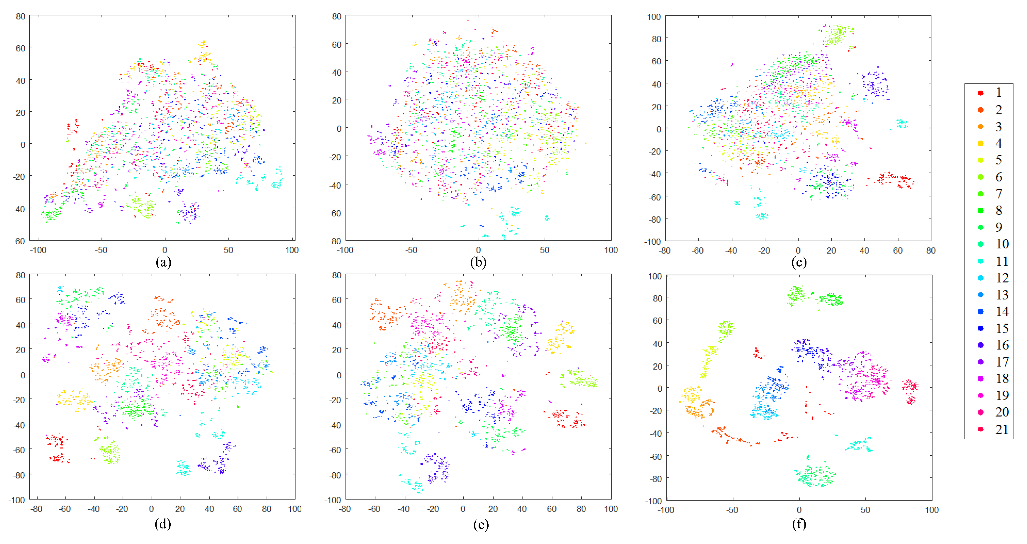
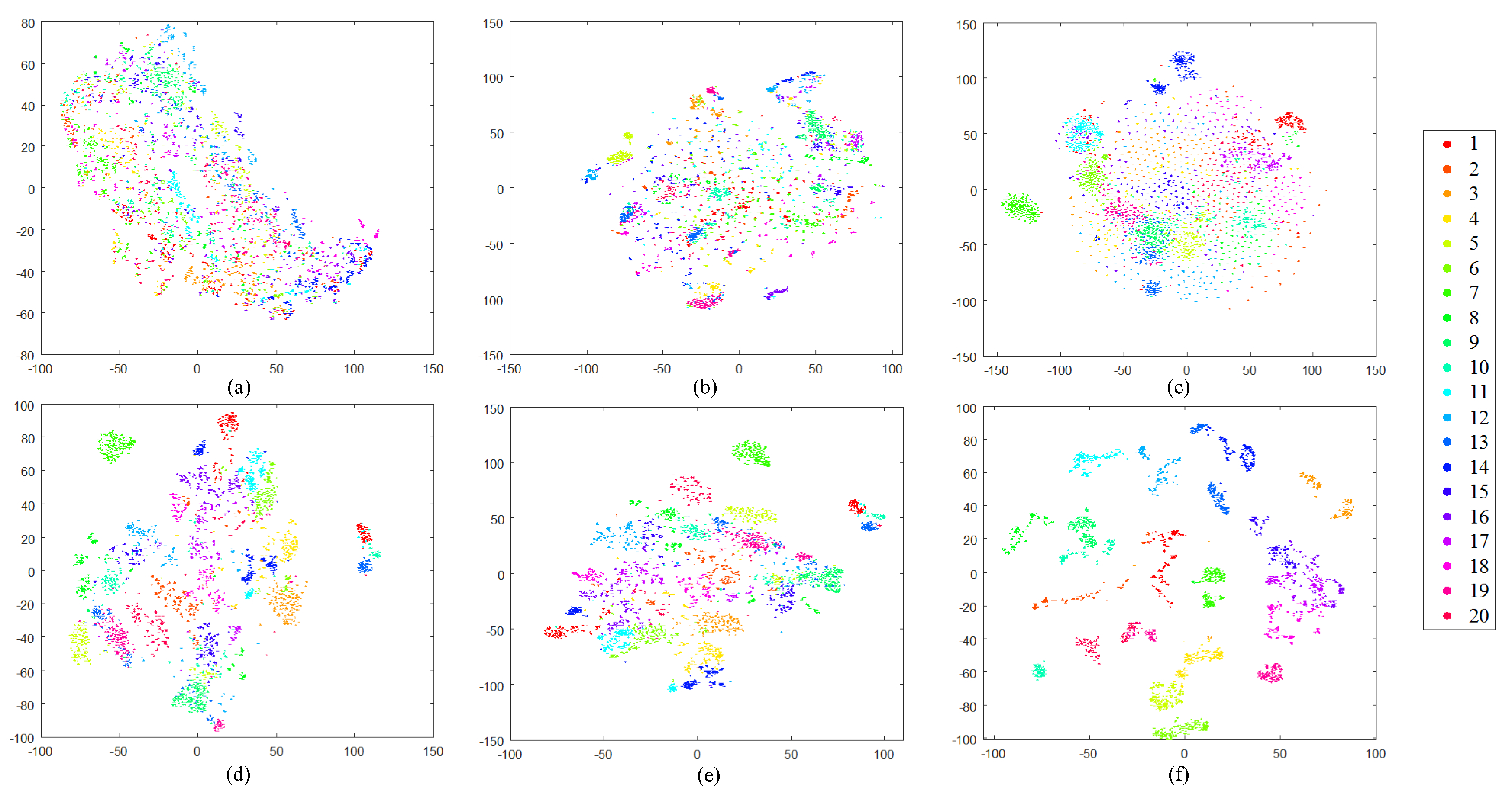
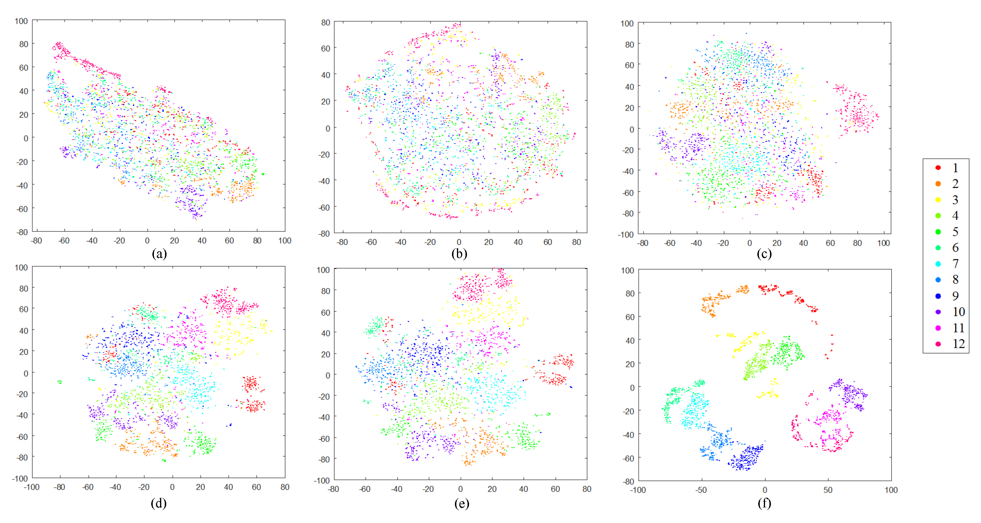
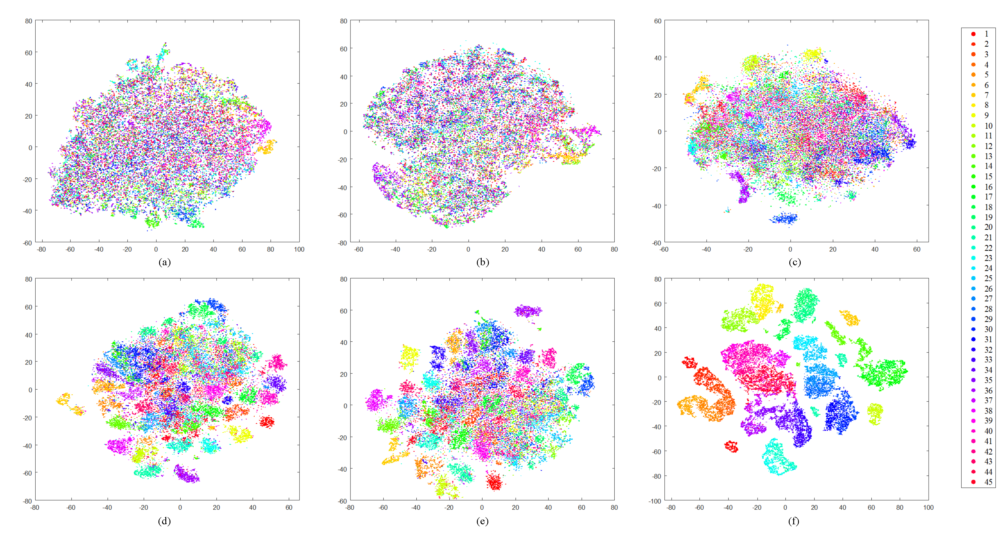
Before providing the numerical assessment, we first study the structure of our DBOW features to visually estimate if they are discriminative enough for RSIR tasks. In this paper, we choose the t-distributed stochastic neighbor embedding (t-SNE) algorithm [57] to reduce the features’ dimension. Then, the structure of features is displayed in the 2-dimensional space. Here, besides the DBOW features, we also exhibit the other four common features’ structure as the reference, including the homogeneous texture (HT) features [15] obtained by Gabor filters, the color histogram (CH) features [45], the SIFT-based BOW (S-BOW) features [23], and the deep network features (DN) extracted using the pre-trained Overfeat net [58]. Note that the DN features mentioned above are the outputs of the seventh and eighth fully connected layers, so that we record them DN-7 and DN-8. The dimensions of six types of features are 1500 (DBOW/S-BOW), 60 (HT), 384 (CH), 4069 (DN-7/8), respectively. To accomplish the t-SNE algorithm, the L1-norm distance is selected for histogrammic features (i.e., DBOW, CH, and S-BOW), and Euclidean distance is adopted for others. The visual results of different RS image archives are shown in Figure 13, Figure 14, Figure 15 and Figure 16.
From the observation of figures, we can find that clusters derived by the low-level features (HT, CH) are mixed together (Figure 13a–b, Figure 14a–b, Figure 15a–b, and Figure 16a–b), which cannot provide enough discriminative information for RSIR. The mid-level features (S-BOW) perform better, which lead to the initial separation among diverse classes (Figure 13c, Figure 14c, Figure 15c, and Figure 16c). However, the information provided by S-BOW features is not adequate to complete the RSIR task with satisfaction. The structure of deep features (DN-7 and DN-8) is clearer than that of low-/mid-level features (Figure 13d–e, Figure 14d–e, Figure 15d–e, and Figure 16d–e). Although the derived clusters reach separable stage, the relative distances between diverse clusters are not distinct enough. This limits their performance on RSIR. Different from the other five kinds of features, the clusters obtained by our DBOW features are separable obviously (Figure 13f, Figure 14f, Figure 15f, and Figure 16f). In addition, the relative distances between different clusters are distinct. This is beneficial to process RS images to an effective content retrieval stage. The encouraging results indicate that the DBOW feature is useful to the RSIR task. The following experiments also prove this point.
4.4. Retrieval Performance
The following RSIR methods are selected to assess the behavior of our DBOW feature on RSIR objectively:
- The RSIR approach developed by the fuzzy similarity measure [41]. To explore useful information of RS images, they are segmented into different regions first. Then, the regions are represented by the fuzzy descriptors, which aims at overcoming the influence of uncertainty and blurry boundaries between segmented regions. Finally, the similarities between RS images are converted into the resemblance between fuzzy vectors, which is accomplished by the region-based fuzzy matching (RFM) measure [41]. We record this method RSIR-RFM for convenience.
- The RSIR method presented in [23]. The S-BOW features are adopted to represent RS images, and L1-norm distance is selected to decide the similarities between RS images. The RSIR results are obtained in accordance with the distance order. Here, the dimension of SBOW features is 1500. We name this method RSIR-SBOW for short.
- The RSIR method based on the hash features [12]. The successful kernel-based hashing method [59] is introduced to encode the RS images. Then, the similarities between images are obtained by hamming distance in the hash space. Here, we set the length of hash code to be 16 bits, and record this method RSIR-Hash for short.
- The RSIR method based on deep features obtained by the pre-trained CNNs [60]. The Overfeat net [58], which is pre-trained using the imageNet dataset [61], is selected to extract the RS images’ features. The outputs of seventh and eighth layers are regarded as the deep features. The Euclidean distance is selected to weigh the similarities between deep features. The RSIR methods based on different deep features are recorded RSIR-DN7 and RSIR-DN8, respectively, and the dimensions of two deep features are 4096.
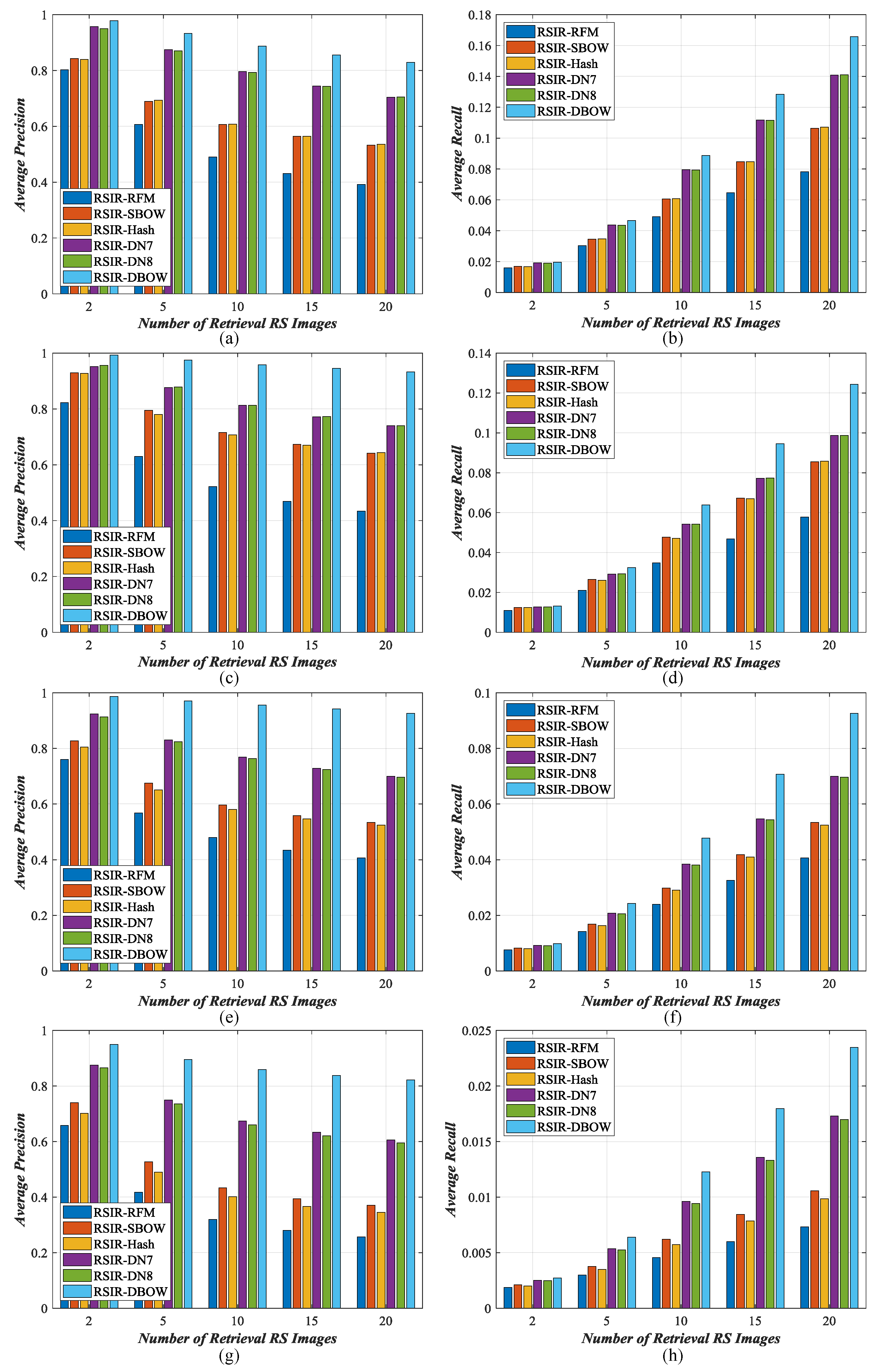
The results of three archives counted on top 20 retrieval images are shown in Figure 17, where our RSIR method is recorded RSIR-DBOW. Note that the parameters of different comparisons are set according to the original literature. From the observation of figures, it is obvious that our RSIR method outperforms other comparisons.
For ImgDB1, the performance of RSIR-RFM is the weakest among the six RSIR methods. This indicates that the region-based representations cannot explore the complex contents within the RS images, which limits their contributions on RSIR. RSIR-SBOW and RSIR-Hash perform better than RSIR-RFM. Their performance is similar to each other. The reason behind this is that they all use SBOW features to represent the RS images, resulting in the captured information from the RS images is similar. Due to the strong capacity of information mining, the features extracted by the pre-trained deep CNNs can describe the RS images clearly, which leads to the stronger performance on RSIR. Compared with three RSIR methods mentioned above, we can easily find that the behavior of RSIR-DN7 and RSIR-DN8 is enhanced to a large degree. An interesting observation is that the performance of RSIR-DN7 and RSIR-DN8 is almost the same, which means that the last two fully connected layers have the similar capacity for feature learning. Although the retrieval results of deep based methods are positive, the performance of them is still weaker than that of our RSIR-DBOW. Moreover, there is a distinct performance gap between our RSIR-DBOW and other comparisons, and the gap becomes larger with the number of retrieval images increases. This proves that the representations learned by our feature learning method can fully explore the complex contents within the RS images, which is beneficial to RSIR tasks. For retrieval precision, comparing with other comparisons, the highest improvements obtained by our method are 43.75% (RSIR-RFM), 29.66% (RSIR-SBOW), 29.30% (RSIR-Hash), 12.46% (RSIR-DN7), and 12.34% (RSIR-DN8). For retrieval recall, the biggest enhancements generated by our method are 8.75% (RSIR-RFM), 5.93% (RSIR-SBOW), 5.86% (RSIR-Hash), 2.49% (RSIR-DN7), and 2.47% (RSIR-DN8).
For the other three image archives, we can find the similar results, i.e., our RSIR-DBOW achieve the best performance compared with all of the comparisons. For ImgDB2, the highest enhancements on retrieval precision/recall generated by our method are 49.93%/6.66% (RSIR-RFM), 29.13%/3.88% (RSIR-SBOW), 28.93%/3.86% (RSIR-Hash), 19.28%/2.57% (RSIR-DN7), and 19.29%/2.58% (RSIR-DN8). For ImgDB3, the biggest improvements on retrieval precision/recall obtained by our method are 51.95%/5.19% (RSIR-RFM), 39.35%/3.93% (RSIR-SBOW), 40.28%/4.03% (RSIR-Hash), 22.66%/2.27% (RSIR-DN7), and 23.06%/2.31% (RSIR-DN8). For ImgDB4, the biggest improvements on retrieval precision/recall obtained by our method are 56.25%/1.61% (RSIR-RFM), 45.13%/1.29% (RSIR-SBOW), 47.66%/1.36% (RSIR-Hash), 21.61%/0.62% (RSIR-DN7), and 22.68%/0.65% (RSIR-DN8).
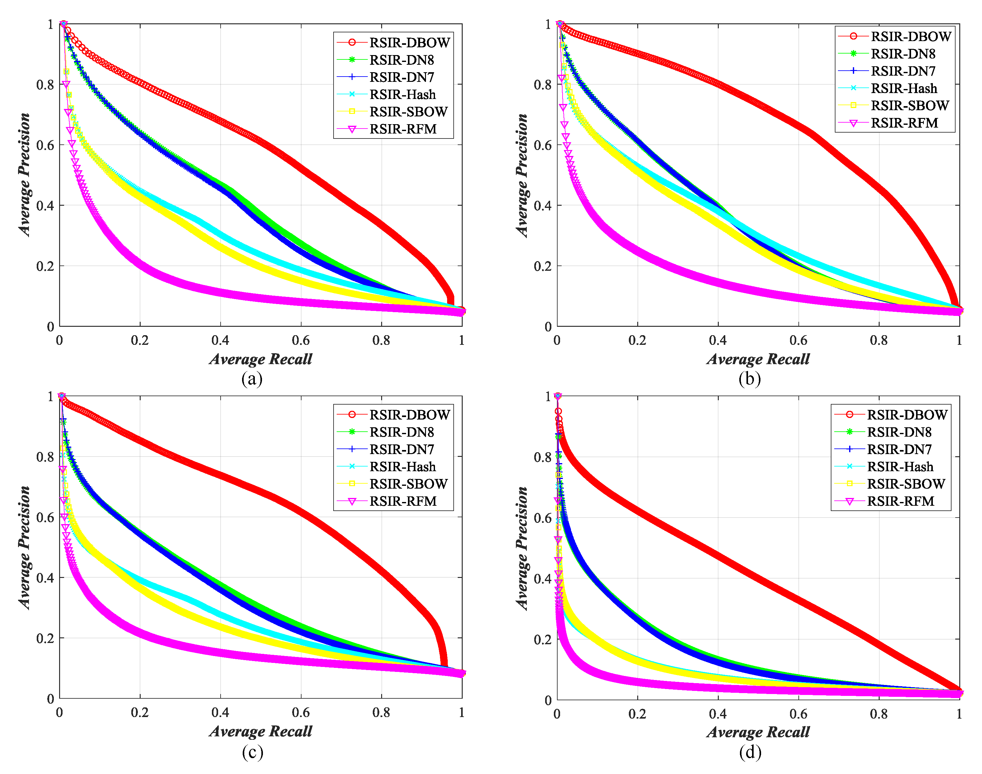
To further study the retrieval performance of our method, we add the recall–precision curve to observe the retrieval behavior with the number of retrieval images increasing. The comparisons’ results are also counted as reference. The results are exhibited in Figure 18. From the observation of curves, we can easily find that our method achieves the best performance on four data sets. These encouraging results illustrate the effectiveness of our RSIR method again.
The retrieval behavior across the different semantic categories is summarized in Table 3, Table 4, Table 5 and Table 6. The results are counted using the top 20 retrieval images. From the observation of these tables, it is obvious that our method performs best in most of the semantic categories. In addition, an encouraging observation is that our RSIR method enhances the retrieval performance to a large degree for many categories, for which other approaches’ behavior is not satisfactory. For example, the retrieval precision of different comparisons for “Dense Residential” within ImgDB1 is less than 0.5, but our method can achieve 0.9595. Furthermore, ImgDB4 is a large-scale RS image data set, no matter on the scene classes or on the total number of images. Our method can still achieve the superior performance on ImgDB4, which proves that our unsupervised feature learning method is useful to RSIR.
4.5. Retrieval Example
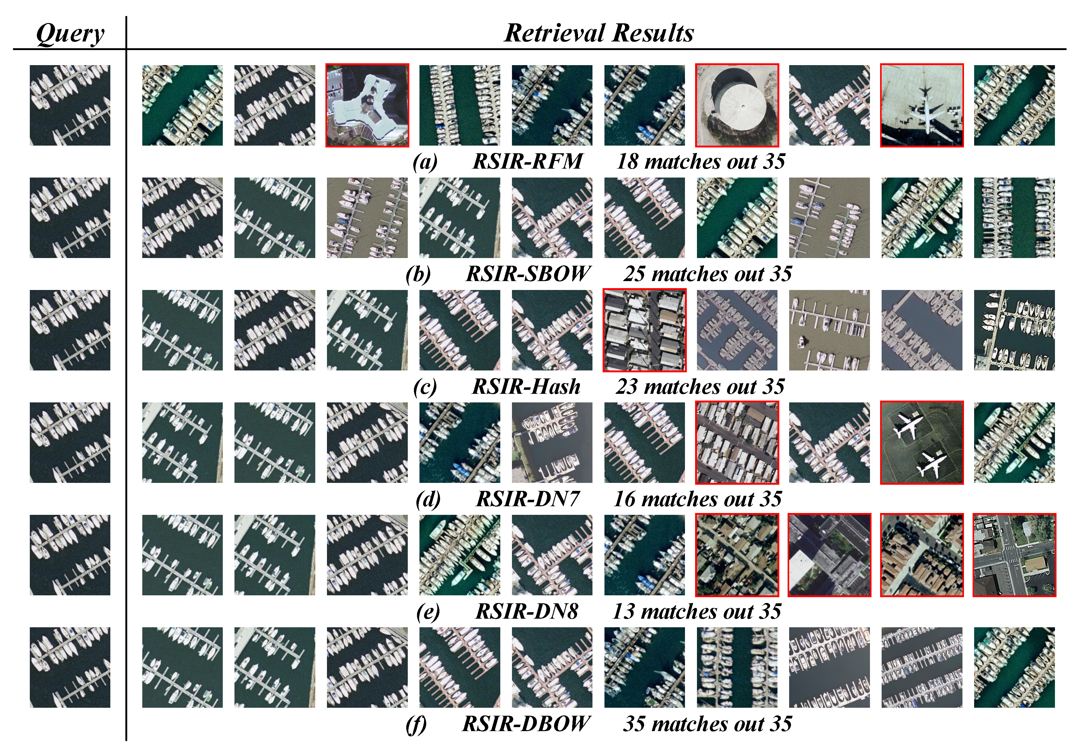
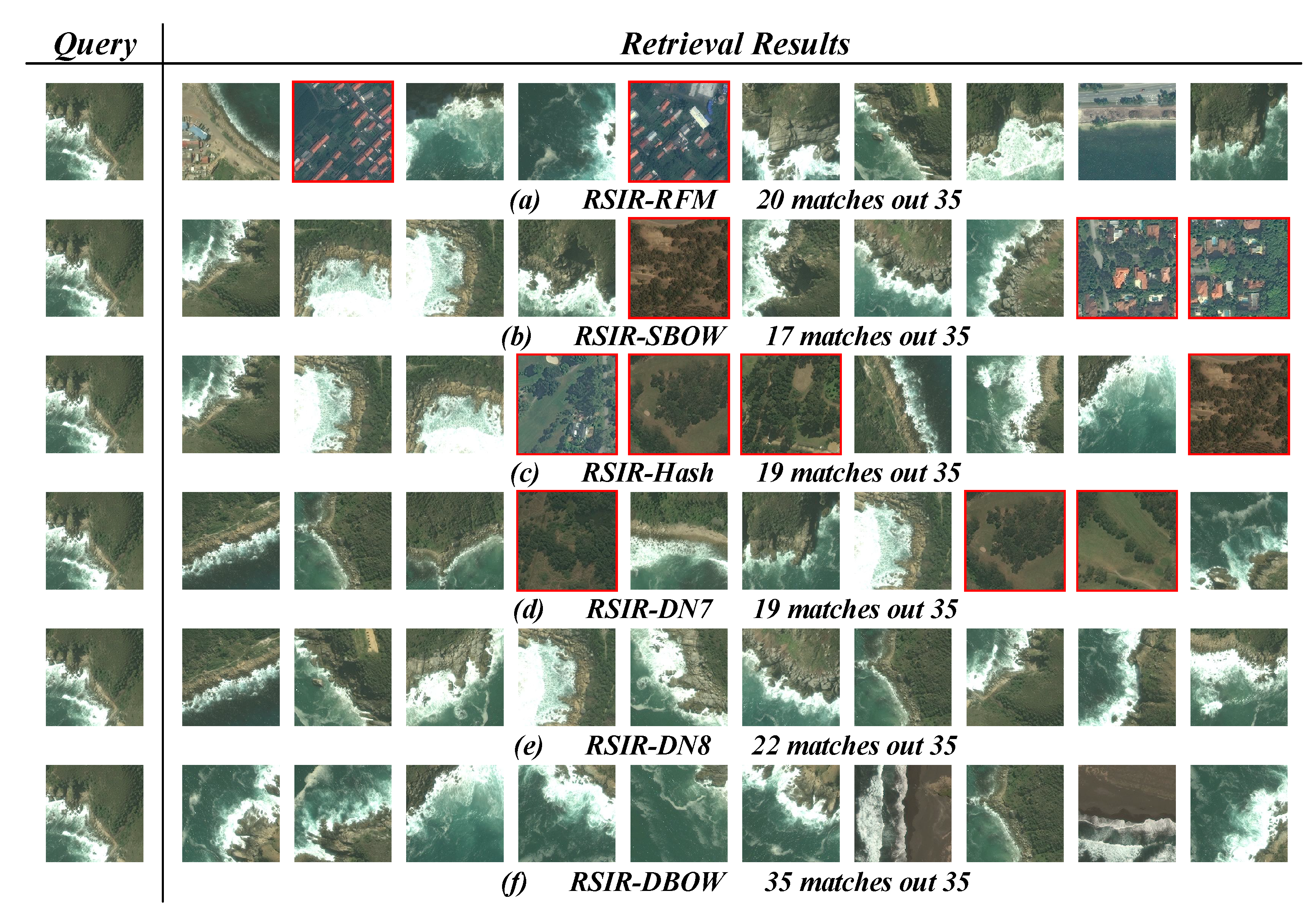
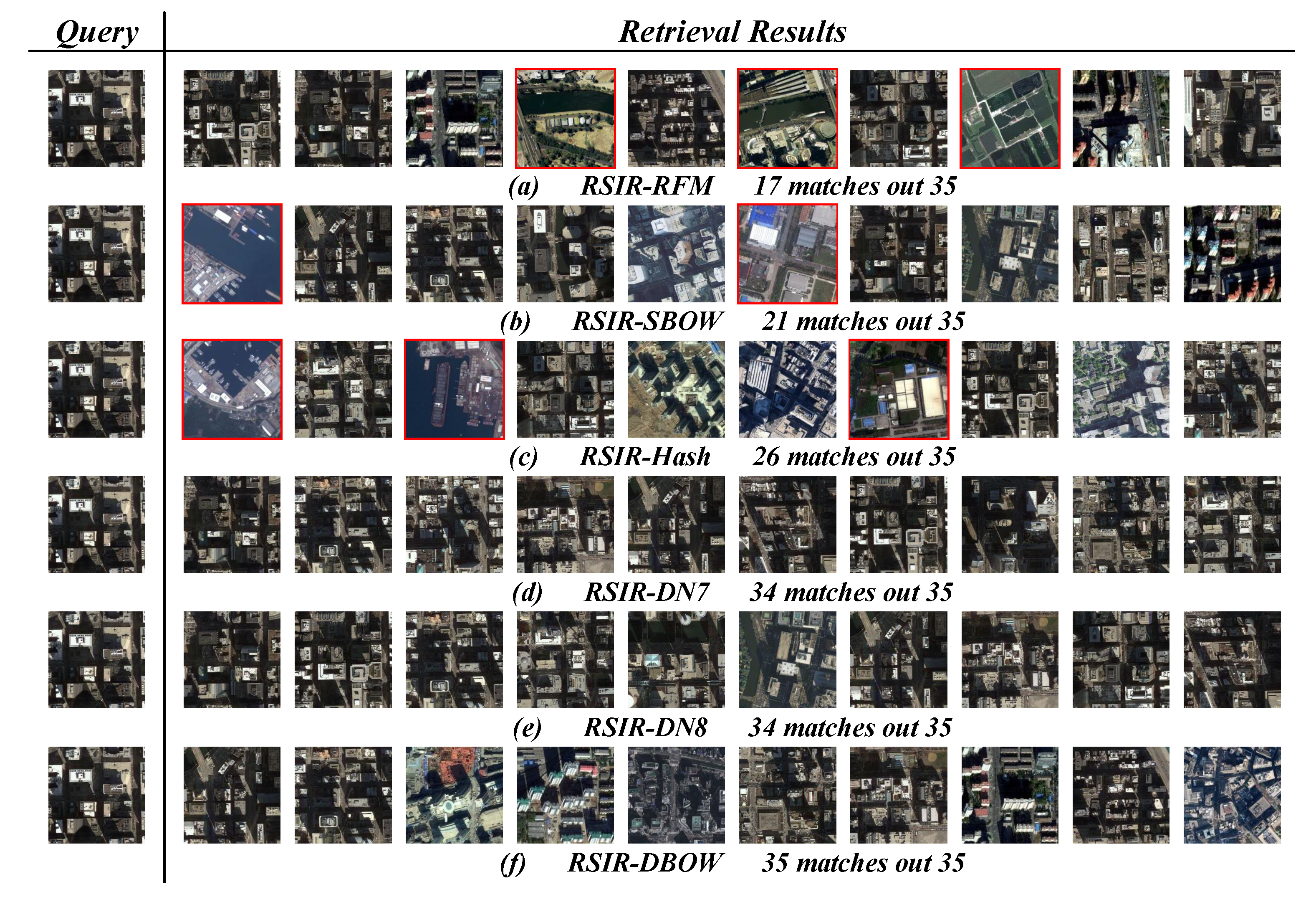
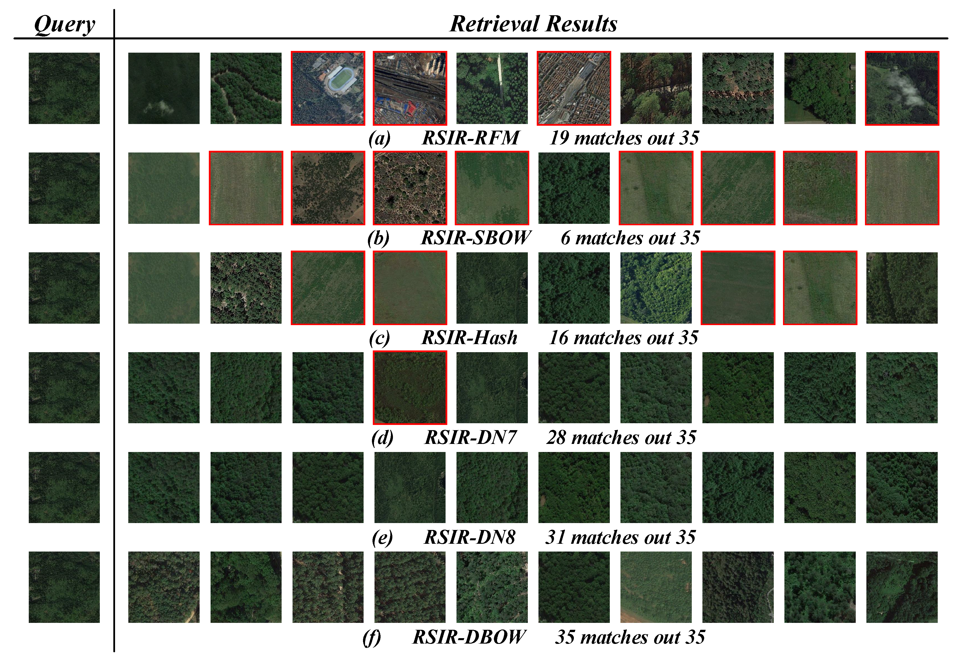
Apart from the numerical assessment, we provide some retrieval examples in this section. Four queries are selected from different RS image archives randomly. Then, different RSIR methods are adopted to acquire the retrieval results. Due to space limitations, only top 10 retrieval images are exhibited in Figure 19, Figure 20, Figure 21 and Figure 22. The incorrect results are tagged in red, and the number of correct retrieval images within top 35 results is provided for reference. From the observation of visual exhibition, we can find that the retrieval performance of our method is the best compared with other approaches. These encouraging experimental results prove the effectiveness of our method again.
4.6. Parameter Analysis
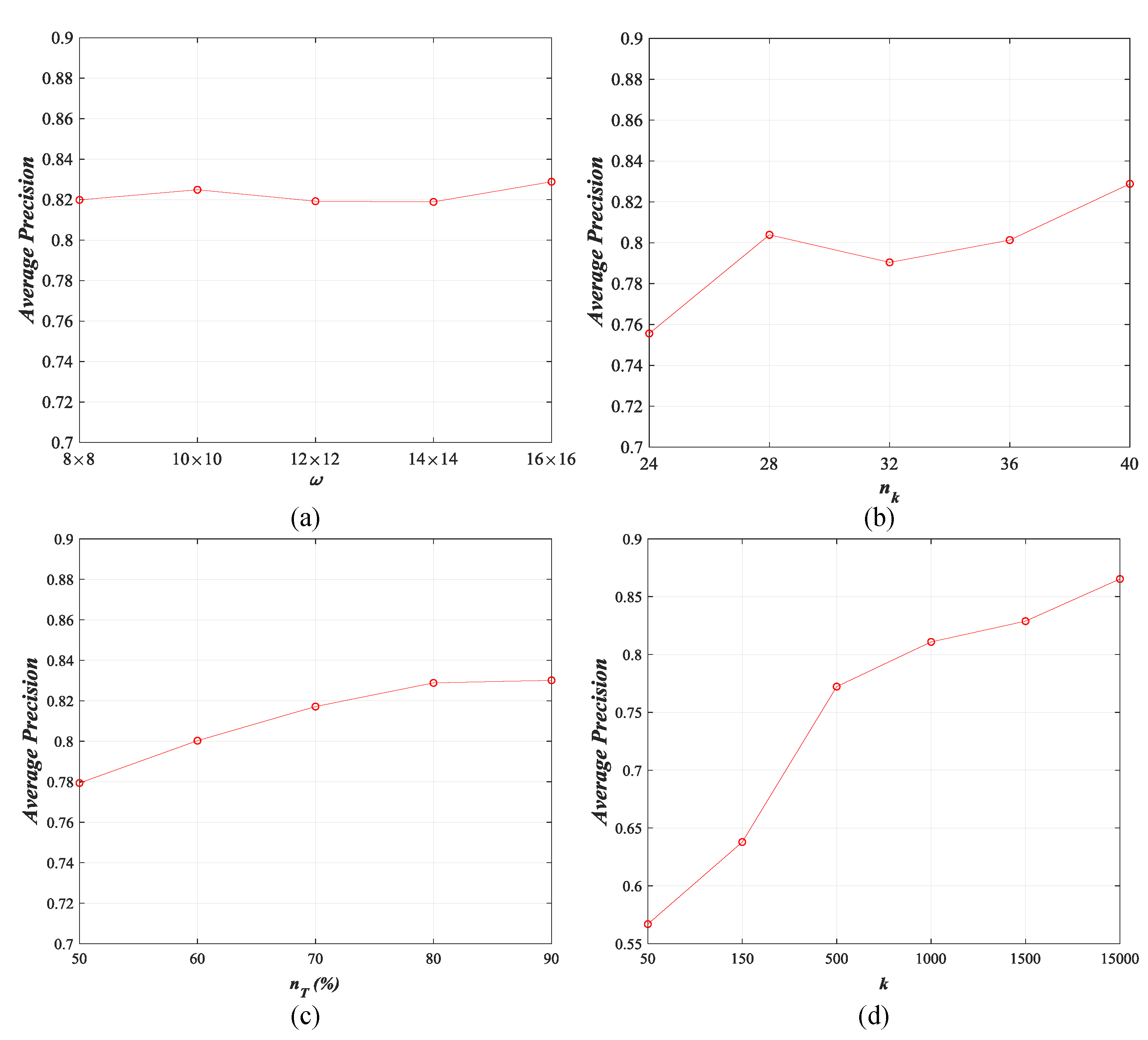
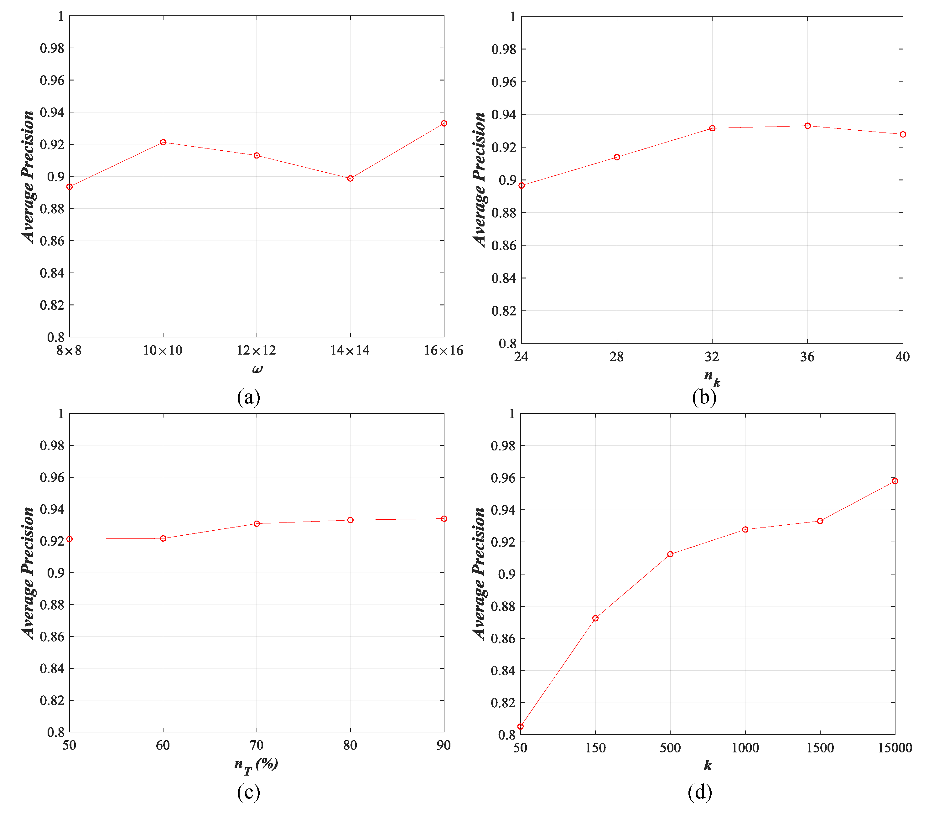
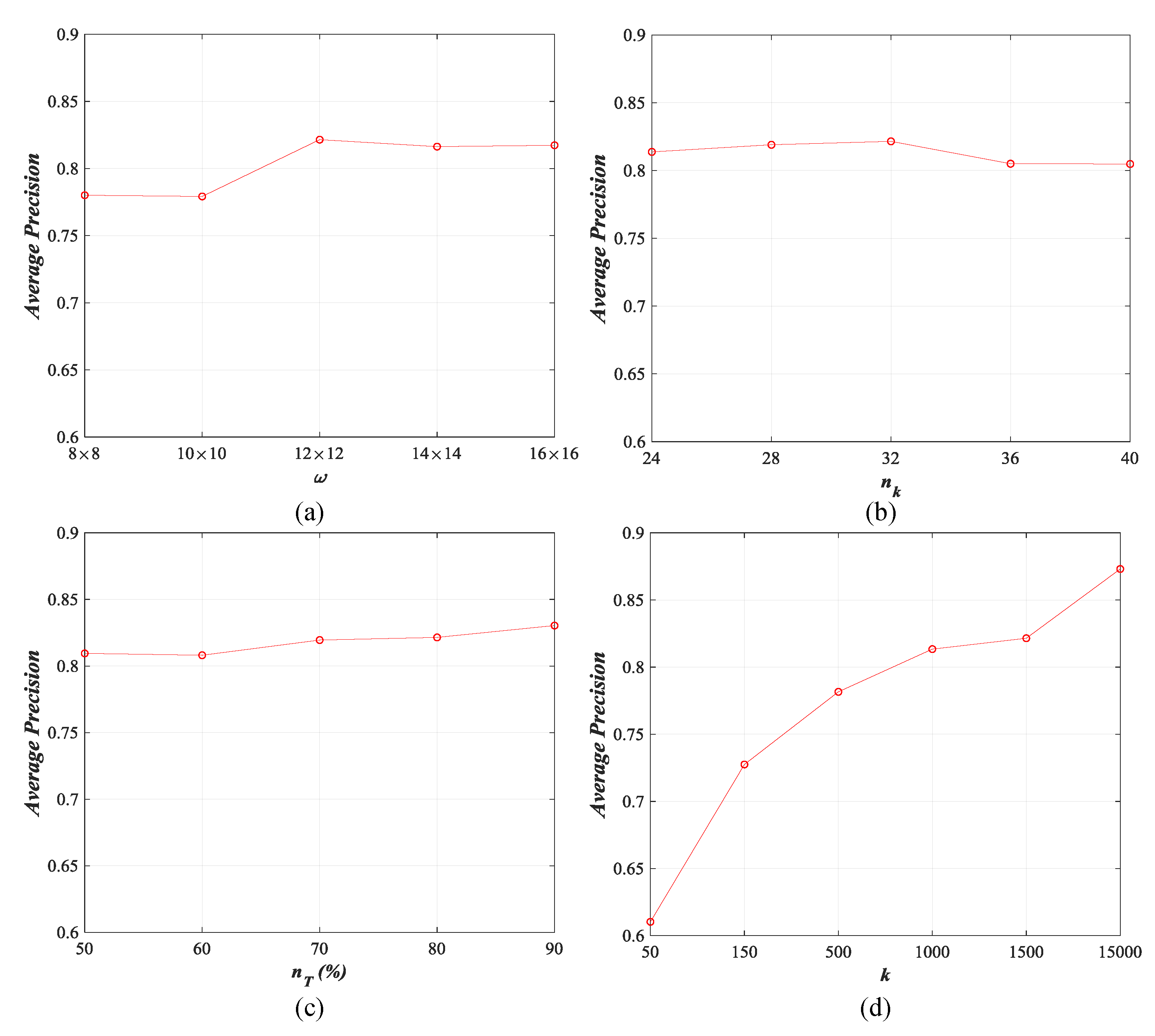
As mentioned in Section 4.1.2, there are four parameters that impact the performance of our DBOW directly, including the size of uniform and superpixel visual words , the number of convolution kernels and the percentage of training set for DCAE training, and the size of codebook k for DBOW generation. In this section, we study the influence of those four parameters in detail through changing their values. The size of visual words is tuned from to with the interval of , the number of convolution kernels is changed from 24 to 40 with the interval of 4, the percentage of training set is varied from 50% to 90% with the interval of 10%, and the size of codebook k is set 50, 150, 500, 1000, 1500, and 1500, respectively. The results of three archives counted using the top-20 retrieval images are exhibited in Figure 23, Figure 24, Figure 25 and Figure 26.
For , the performance of our method is fluctuated within an acceptable range, and the peak values are reached when (ImgDB1, ImgDB2, and ImgDB3) and (ImgDB4). For , the whole trend of our method’s behavior is rising with increases. For different archives, the highest retrieval performance appears at for ImgDB1, for ImgDB2 and ImgDB3, and for ImgDB4. For , more training samples lead to more accurate retrieval results. Nevertheless, more training samples results in longer training time. In addition, the performance is enhanced slightly when for both of the data sets. Thus, we set in this paper. For k, it is obvious that the performance of our method is getting better when the value of k increases. However, the computational complexity will be increased dramatically when . Therefore, we set in this paper to balance the performance and the computational complexity.
4.7. Computational Cost
Apart from the average retrieval precision and recall, the computation cost is another important assessment criteria for the RSIR methods. In this section, we discuss the computational cost of our method. As mentioned in Section 3, the RSIR method proposed in this paper consists of two parts, including DBOW feature learning and similarity matching. Therefore, we study the computational cost from those two aspects.
The process of DBOW feature learning can be split into offline training and online feature learning. The offline training process is time consuming. Taking ImgDB1 as an example, when the proportion of the training set equals 80% (more than 600,000 image patches with size of ), we need almost 40 min to train our DCAE models and generate the codebook using different kinds of visual words. After the model training, the offline feature extraction process is fast, which just needs around 300 milliseconds for a RS image.
For similarity matching, the common distance metric is used to measure the similarities between query and target images, and the exhaustive search through linear scan is used to obtain the retrieval results. The time cost of this part is impacted by the size of image archive and the dimension of image feature directly. Here, we further study the computational cost of similarity matching through changing the size of target archive. The time cost of different comparisons is also counted as the reference. The experimental results are shown in Table 7. From the observation of the values, we can find that the most time-consuming method is RSIR-RFM. The reason is that the feature used in RFM measure is discrete distribution rather than the single vector. The fastest method is RSIR-Hash since the hashing code is the binary feature, and the similarities between hashing features can be calculated by the bit operation. For other RSIR methods, the similarity matching time cost is proportional to the feature dimension.
5. Conclusions
This paper presents an unsupervised deep feature learning method for the RSIR task. First, we use the image patches rather than the whole image to explore the diverse contents within the RS image. In addition, considering the multi-scale property of objects, two region sampling schemes are adopted for generating the patches with different sizes. Second, instead of using the low-/mid-level representations, the DCAE model is introduced to learn the latent features from the patches. This guarantees that the acquired features are discriminative enough to be the image descriptors. Third, all of the deep descriptors are used to generate the codebook using the k-means algorithm. Finally, the histogrammic DBOW features are constructed by counting the frequency of the single codewords. The RSIR results can be obtained according to the L1-norm distances between DBOW features directly. The encouraging experimental results of four RS image archives prove that our deep feature is effective for the RSIR task.
Although the proposed feature learning method performs positively for RSIR tasks, its shortcomings are obvious enough that we cannot neglect them. Since there are two sets of patches for an RS image, the contents within the patches belonging to different sets may be overlapped. Thus, the convolution operation is performed several times on some overlapping patches from one image, which is redundant in computation. How to overcome this limitation for reducing the computation cost is one of our future focuses.
Author Contributions
X.T. designed the project, oversaw the analysis, and wrote the manuscript; X.Z. and F.L. analyzed the data; L.J. improved the manuscript.
Funding
This work was supported in part by the China Postdoctoral Science Foundation funded projects (No. 2017M620441, 2017M623126), the National Science Basic Research Plan in Shaanxi Province of China (No. 2018JQ6018), the National Natural Science Foundation of China (No. 61772400), and the Xidian University New Teacher Innovation Fund Project (No. XJS18032).
Acknowledgments
The authors would like to show their gratitude to the editors and the anonymous reviewers for their comments and suggestions.
Conflicts of Interest
The authors declare no conflict of interest.
References
- Quartulli, M.; Olaizola, I.G. A review of EO image information mining. J. Photogram. Remote Sens. 2013, 75, 11–28. [Google Scholar] [CrossRef] [Green Version]
- Datcu, M.; Daschiel, H.; Pelizzari, A.; Quartulli, M.; Galoppo, A.; Colapicchioni, A.; Pastori, M.; Seidel, K.; Marchetti, P.G.; d’Elia, S. Information mining in remote sensing image archives: System concepts. IEEE Trans. Geosci. Remote Sens. 2003, 41, 2923–2936. [Google Scholar] [CrossRef]
- Datta, R.; Joshi, D.; Li, J.; Wang, J.Z. Image retrieval: Ideas, influences, and trends of the new age. ACM Comput. Surv. 2008, 40, 5. [Google Scholar] [CrossRef]
- Wang, J.Z.; Li, J.; Wiederhold, G. SIMPLIcity: Semantics-sensitive integrated matching for picture libraries. IEEE Trans. Pattern Anal. Mach. Intell. 2001, 23, 947–963. [Google Scholar] [CrossRef]
- Chen, Y.; Wang, J.Z.; Krovetz, R. CLUE: Cluster-based retrieval of images by unsupervised learning. IEEE Trans. Image Process. 2005, 14, 1187–1201. [Google Scholar] [CrossRef] [PubMed]
- Yu, J.; Yang, X.; Gao, F.; Tao, D. Deep multimodal distance metric learning using click constraints for image ranking. IEEE Trans. Cybern. 2017, 47, 4014–4024. [Google Scholar] [CrossRef] [PubMed]
- Napoletano, P. Visual descriptors for content-based retrieval of remote-sensing images. Int. J. Remote Sens. 2018, 39, 1343–1376. [Google Scholar] [CrossRef]
- Lu, X.; Zheng, X.; Yuan, Y. Remote sensing scene classification by unsupervised representation learning. IEEE Trans. Geosci. Remote Sens. 2017, 55, 5148–5157. [Google Scholar] [CrossRef]
- Tao, Y.; Xu, M.; Zhang, F.; Du, B.; Zhang, L. Unsupervised-Restricted Deconvolutional Neural Network for Very High Resolution Remote-Sensing Image Classification. IEEE Trans. Geosci. Remote Sens. 2017, 55, 6805–6823. [Google Scholar] [CrossRef]
- Wang, Q.; He, X.; Li, X. Locality and Structure Regularized Low Rank Representation for Hyperspectral Image Classification. IEEE Trans. Geosci. Remote Sens. 2018, 1–13. [Google Scholar]
- Wang, Q.; Zhang, F.; Li, X. Optimal Clustering Framework for Hyperspectral Band Selection. IEEE Trans. Geosci. Remote Sens. 2018, PP, 1–13. [Google Scholar] [CrossRef]
- Demir, B.; Bruzzone, L. Hashing-based scalable remote sensing image search and retrieval in large archives. IEEE Trans. Geosci. Remote Sens. 2016, 54, 892–904. [Google Scholar] [CrossRef]
- Haralick, R.M.; Shanmugam, K.; Dinstein, I. Textural features for image classification. IEEE Trans. Syst. Man Cybern. 1973, SMC-3, 610–621. [Google Scholar]
- Zhang, X.; Jiao, L.; Liu, F.; Bo, L.; Gong, M. Spectral clustering ensemble applied to SAR image segmentation. IEEE Trans. Geosci. Remote Sens. 2008, 46, 2126–2136. [Google Scholar] [CrossRef]
- Manjunath, B.S.; Salembier, P.; Sikora, T. Introduction to MPEG-7: Multimedia Content Description Interface; John Wiley & Sons: New York, NY, USA, 2002; Volume 1. [Google Scholar]
- Sivic, J.; Zisserman, A. Video Google: A text retrieval approach to object matching in videos. In Proceedings of the 9th IEEE International Conference on Computer Vision, Nice, France, 13–16 October 2003; p. 1470. [Google Scholar]
- Krizhevsky, A.; Sutskever, I.; Hinton, G.E. Imagenet classification with deep convolutional neural networks. In Proceedings of the Advances in Neural Information Processing Systems, Lake Tahoe, NV, USA, 3–6 December 2012; pp. 1097–1105. [Google Scholar]
- Simonyan, K.; Zisserman, A. Very deep convolutional networks for large-scale image recognition. arXiv 2014, arXiv:1409.1556. [Google Scholar]
- Gong, M.; Zhao, J.; Liu, J.; Miao, Q.; Jiao, L. Change detection in synthetic aperture radar images based on deep neural networks. IEEE Trans. Neural Netw. Learn. Syst. 2016, 27, 125–138. [Google Scholar] [CrossRef] [PubMed]
- Zhang, X.; Liang, Y.; Li, C.; Huyan, N.; Jiao, L.; Zhou, H. Recursive Autoencoders-Based Unsupervised Feature Learning for Hyperspectral Image Classification. IEEE Geosci. Remote Sens. Lett. 2017, 14, 1928–1932. [Google Scholar] [CrossRef] [Green Version]
- Liu, X.; Jiao, L.; Zhao, J.; Zhao, J.; Zhang, D.; Liu, F.; Yang, S.; Tang, X. Deep Multiple Instance Learning-Based Spatial-Spectral Classification for PAN and MS Imagery. IEEE Trans. Geosci. Remote Sens. 2018, 56, 461–473. [Google Scholar] [CrossRef]
- Wang, Q.; Yuan, Z.; Li, X. GETNET: A General End-to-end Two-dimensional CNN Framework for Hyperspectral Image Change Detection. IEEE Trans. Geosci. Remote Sens. 2018. [Google Scholar] [CrossRef]
- Yang, Y.; Newsam, S. Geographic image retrieval using local invariant features. IEEE Trans. Geosci. Remote Sens. 2013, 51, 818–832. [Google Scholar] [CrossRef]
- Yang, Y.; Newsam, S. Bag-of-visual-words and spatial extensions for land-use classification. In Proceedings of the 18th SIGSPATIAL International Conference on Advances in Geographic Information Systems, San Jose, CA, USA, 3–5 November 2010; pp. 270–279. [Google Scholar]
- Bai, Y.; Yu, W.; Xiao, T.; Xu, C.; Yang, K.; Ma, W.Y.; Zhao, T. Bag-of-words based deep neural network for image retrieval. In Proceedings of the 22nd ACM international conference on Multimedia, Orlando, FL, USA, 3–7 November 2014; pp. 229–232. [Google Scholar]
- Leskovec, J.; Rajaraman, A.; Ullman, J.D. Mining of Massive Datasets; Cambridge University Press: Cambridge, UK, 2014. [Google Scholar]
- Datcu, M.; Seidel, K.; Walessa, M. Spatial information retrieval from remote-sensing images. I. Information theoretical perspective. IEEE Trans. Geosci. Remote Sens. 1998, 36, 1431–1445. [Google Scholar] [CrossRef]
- Schroder, M.; Rehrauer, H.; Seidel, K.; Datcu, M. Spatial information retrieval from remote-sensing images. II. Gibbs-Markov random fields. IEEE Trans. Geosci. Remote Sens. 1998, 36, 1446–1455. [Google Scholar] [CrossRef]
- Daschiel, H.; Datcu, M.P. Cluster structure evaluation of dyadic k-means for mining large image archives. In Proceedings of the Image and Signal Processing for Remote Sens. VIII. International Society for Optics and Photonics, Crete, Greece, 13 March 2003; Volume 4885, pp. 120–131. [Google Scholar]
- Shyu, C.R.; Klaric, M.; Scott, G.J.; Barb, A.S.; Davis, C.H.; Palaniappan, K. GeoIRIS: Geospatial information retrieval and indexing system—Content mining, semantics modeling, and complex queries. IEEE Trans. Geosci. Remote Sens. 2007, 45, 839–852. [Google Scholar] [CrossRef] [PubMed]
- Lowe, D.G. Object recognition from local scale-invariant features. In Proceedings of the Seventh IEEE International Conference on Computer Vision, Kerkyra, Greece, 20–27 September 1999; Volume 2, pp. 1150–1157. [Google Scholar]
- Lowe, D.G. Distinctive image features from scale-invariant keypoints. Int. J. Comput. Vis. 2004, 60, 91–110. [Google Scholar] [CrossRef]
- Aptoula, E. Remote sensing image retrieval with global morphological texture descriptors. IEEE Trans. Geosci. Remote Sens. 2014, 52, 3023–3034. [Google Scholar] [CrossRef]
- Pham, M.T.; Mercier, G.; Regniers, O.; Michel, J. Texture retrieval from VHR optical remote sensed images using the local extrema descriptor with application to vineyard parcel detection. Remote Sens. 2016, 8, 368. [Google Scholar] [CrossRef] [Green Version]
- Zhou, W.; Shao, Z.; Diao, C.; Cheng, Q. High-resolution remote-sensing imagery retrieval using sparse features by auto-encoder. Remote Sens. Lett. 2015, 6, 775–783. [Google Scholar] [CrossRef]
- Li, Y.; Zhang, Y.; Tao, C.; Zhu, H. Content-based high-resolution remote sensing image retrieval via unsupervised feature learning and collaborative affinity metric fusion. Remote Sens. 2016, 8, 709. [Google Scholar] [CrossRef]
- Zhou, W.; Newsam, S.; Li, C.; Shao, Z. Learning low dimensional convolutional neural networks for high-resolution remote sensing image retrieval. Remote Sens. 2017, 9, 489. [Google Scholar] [CrossRef]
- Li, Y.; Zhang, Y.; Huang, X.; Zhu, H.; Ma, J. Large-scale remote sensing image retrieval by deep hashing neural networks. IEEE Trans. Geosci. Remote Sens. 2018, 56, 950–965. [Google Scholar] [CrossRef]
- Datta, R.; Li, J.; Parulekar, A.; Wang, J.Z. Scalable remotely sensed image mining using supervised learning and content-based retrieval. Tech. Rep. CSE 2006, 6–19. Available online: https://pdfs.semanticscholar.org/4438/012b243ad7e1741e0e111d68b0b5d3ce31f0.pdf (accessed on 9 June 2012).
- Jiao, L.; Tang, X.; Hou, B.; Wang, S. SAR images retrieval based on semantic classification and region-based similarity measure for earth observation. IEEE J. Sel. Top. Appl. Earth Obs. Remote Sens. 2015, 8, 3876–3891. [Google Scholar] [CrossRef]
- Tang, X.; Jiao, L.; Emery, W.J. SAR image content retrieval based on fuzzy similarity and relevance feedback. IEEE J. Sel. Top. Appl. Earth Obs. Remote Sens. 2017, 10, 1824–1842. [Google Scholar] [CrossRef]
- Scott, G.J.; Klaric, M.N.; Davis, C.H.; Shyu, C.R. Entropy-balanced bitmap tree for shape-based object retrieval from large-scale satellite imagery databases. IEEE Trans. Geosci. Remote Sens. 2011, 49, 1603–1616. [Google Scholar] [CrossRef]
- Wang, Y.; Zhang, L.; Tong, X.; Zhang, L.; Zhang, Z.; Liu, H.; Xing, X.; Mathiopoulos, P.T. A three-layered graph-based learning approach for remote sensing image retrieval. IEEE Trans. Geosci. Remote Sens. 2016, 54, 6020–6034. [Google Scholar] [CrossRef]
- Tang, X.; Jiao, L. Fusion similarity-based reranking for SAR image retrieval. IEEE Geosci. Remote Sens. Lett. 2017, 14, 242–246. [Google Scholar] [CrossRef]
- Tang, X.; Jiao, L.; Emery, W.J.; Liu, F.; Zhang, D. Two-stage reranking for remote sensing image retrieval. IEEE Trans. Geosci. Remote Sens. 2017, 55, 5798–5817. [Google Scholar] [CrossRef]
- Masci, J.; Meier, U.; Cireşan, D.; Schmidhuber, J. Stacked convolutional auto-encoders for hierarchical feature extraction. In Proceedings of the International Conference on Artificial Neural Networks, Espoo, Finland, 14–17 June 2011; pp. 52–59. [Google Scholar]
- Csurka, G.; Dance, C.; Fan, L.; Willamowski, J.; Bray, C. Visual categorization with bags of keypoints. In Proceedings of the 8th European Conference on Computer Vision, Prague, Czech Republic, 11–14 May 2004; Volume 1, pp. 1–2. [Google Scholar]
- Zhu, Q.; Zhong, Y.; Zhao, B.; Xia, G.S.; Zhang, L. Bag-of-visual-words scene classifier with local and global features for high spatial resolution remote sensing imagery. IEEE Geosci. Remote Sens. Lett. 2016, 13, 747–751. [Google Scholar] [CrossRef]
- Hu, J.; Xia, G.S.; Hu, F.; Zhang, L. A comparative study of sampling analysis in the scene classification of optical high-spatial resolution remote sensing imagery. Remote Sens. 2015, 7, 14988–15013. [Google Scholar] [CrossRef]
- Veksler, O.; Boykov, Y.; Mehrani, P. Superpixels and supervoxels in an energy optimization framework. In Proceedings of the 11th European Conference on Computer Vision, Heraklion, Crete, Greece, 5–11 September 2010; pp. 211–224. [Google Scholar]
- Achanta, R.; Süsstrunk, S. Superpixels and polygons using simple non-iterative clustering. In Proceedings of the 2017 IEEE Conference on Computer Vision and Pattern Recognition (CVPR), Honolulu, HI, USA, 21–26 July 2017; pp. 4895–4904. [Google Scholar]
- Achanta, R.; Shaji, A.; Smith, K.; Lucchi, A.; Fua, P.; Süsstrunk, S. SLIC superpixels compared to state-of-the-art superpixel methods. IEEE Trans. Pattern Anal. Mach. Intell. 2012, 34, 2274–2282. [Google Scholar] [CrossRef] [PubMed]
- Lee, H.; Grosse, R.; Ranganath, R.; Ng, A.Y. Convolutional deep belief networks for scalable unsupervised learning of hierarchical representations. In Proceedings of the 26th Annual International Conference on Machine Learning, Montreal, QC, Canada, 14–18 June 2009; pp. 609–616. [Google Scholar]
- Zhao, B.; Zhong, Y.; Xia, G.S.; Zhang, L. Dirichlet-derived multiple topic scene classification model for high spatial resolution remote sensing imagery. IEEE Trans. Geosci. Remote Sens. 2016, 54, 2108–2123. [Google Scholar] [CrossRef]
- Zhao, B.; Zhong, Y.; Zhang, L.; Huang, B. The Fisher kernel coding framework for high spatial resolution scene classification. Remote Sens. 2016, 8, 157. [Google Scholar] [CrossRef]
- Cheng, G.; Han, J.; Lu, X. Remote sensing image scene classification: Benchmark and state of the art. Proc. IEEE 2017, 105, 1865–1883. [Google Scholar] [CrossRef]
- Maaten, L.V.D.; Hinton, G. Visualizing data using t-SNE. J. Mach. Learn. Res. 2008, 9, 2579–2605. [Google Scholar]
- Sermanet, P.; Eigen, D.; Zhang, X.; Mathieu, M.; Fergus, R.; LeCun, Y. Overfeat: Integrated recognition, localization and detection using convolutional networks. arXiv 2013, arXiv:1312.6229. [Google Scholar]
- Kulis, B.; Grauman, K. Kernelized locality-sensitive hashing. IEEE Trans. Pattern Anal. Mach. Intell. 2012, 34, 1092–1104. [Google Scholar] [CrossRef] [PubMed]
- Marmanis, D.; Datcu, M.; Esch, T.; Stilla, U. Deep learning earth observation classification using ImageNet pretrained networks. IEEE Geosci. Remote Sens. Lett. 2016, 13, 105–109. [Google Scholar] [CrossRef]
- Deng, J.; Dong, W.; Socher, R.; Li, L.J.; Li, K.; Li, F. Imagenet: A large-scale hierarchical image database. In Proceedings of the 2009 IEEE Conference on Computer Vision and Pattern Recognition, Miami, FL, USA, 20–25 June 2009; pp. 248–255. [Google Scholar]
Figure 1.
Basic flowchart of the remote sensing image retrieval method.

Figure 2.
Complex contents within one remote sensing image. The main body of this remote sensing image is “Freeway”. Apart from “Freeway”, there are also “Vehicle”, “Tree”, “Building”, “Parking lot”, etc. In addition, the scales of the same targets are different.
Figure 2.
Complex contents within one remote sensing image. The main body of this remote sensing image is “Freeway”. Apart from “Freeway”, there are also “Vehicle”, “Tree”, “Building”, “Parking lot”, etc. In addition, the scales of the same targets are different.

Figure 3.
Three “Agricultural” remote sensing images selected from the UCMerced archive randomly: (a) Agricultural02; (b) Agricultural03; (c) Agricultural04.
Figure 3.
Three “Agricultural” remote sensing images selected from the UCMerced archive randomly: (a) Agricultural02; (b) Agricultural03; (c) Agricultural04.

Figure 4.
Framework of RSIR based on the proposed feature learning method.

Figure 5.
Framework of a convolutional auto-encoder.

Figure 6.
Framework of the proposed patch based deep descriptor learning.

Figure 7.
Framework of the utilized deep convolutional auto-encoder.

Figure 8.
Pipeline of deep bag-of-words generation.

Figure 9.
Examples of ImgDB1.

Figure 10.
Examples of ImgDB2.

Figure 11.
Examples of ImgDB3.

Figure 12.
Examples of ImgDB4.

Figure 13.
Two-dimensional scatterplots of different high-dimensional features obtained by t-SNE over ImgDB1 with 21 semantic classes. The relationships between number ID and semantics can be found in Figure 9. (a) HT; (b) CH; (c) S-BOW; (d) DN-7; (e) DN-8; (f) DBOW.
Figure 13.
Two-dimensional scatterplots of different high-dimensional features obtained by t-SNE over ImgDB1 with 21 semantic classes. The relationships between number ID and semantics can be found in Figure 9. (a) HT; (b) CH; (c) S-BOW; (d) DN-7; (e) DN-8; (f) DBOW.

Figure 14.
Two-dimensional scatterplots of different high-dimensional features obtained by t-SNE over ImgDB2 with 20 semantic classes. The relationships between number ID and semantics can be found in Figure 10. (a) HT; (b) CH; (c) S-BOW; (d) DN-7; (e) DN-8; (f) DBOW.
Figure 14.
Two-dimensional scatterplots of different high-dimensional features obtained by t-SNE over ImgDB2 with 20 semantic classes. The relationships between number ID and semantics can be found in Figure 10. (a) HT; (b) CH; (c) S-BOW; (d) DN-7; (e) DN-8; (f) DBOW.

Figure 15.
Two-dimensional scatterplots of different high-dimensional features obtained by t-SNE over ImgDB3 with 12 semantic classes. The relationships between number ID and semantics can be found in Figure 11. (a) HT; (b) CH; (c) S-BOW; (d) DN-7; (e) DN-8; (f) DBOW.
Figure 15.
Two-dimensional scatterplots of different high-dimensional features obtained by t-SNE over ImgDB3 with 12 semantic classes. The relationships between number ID and semantics can be found in Figure 11. (a) HT; (b) CH; (c) S-BOW; (d) DN-7; (e) DN-8; (f) DBOW.

Figure 16.
Two-dimensional scatterplots of different high-dimensional features obtained by t-SNE over ImgDB4 with 45 semantic classes. The relationships between number ID and semantics can be found in Figure 12. (a) HT; (b) CH; (c) S-BOW; (d) DN-7; (e) DN-8; (f) DBOW.
Figure 16.
Two-dimensional scatterplots of different high-dimensional features obtained by t-SNE over ImgDB4 with 45 semantic classes. The relationships between number ID and semantics can be found in Figure 12. (a) HT; (b) CH; (c) S-BOW; (d) DN-7; (e) DN-8; (f) DBOW.

Figure 17.
Retrieval performance of different RSIR methods on four RS image sets. (a) average retrieval precision on ImgDB1; (b) average retrieval recall on ImgDB1; (c) average retrieval precision on ImgDB2; (d) average retrieval recall on ImgDB2; (e) average retrieval precision on ImgDB3; (f) average retrieval recall on ImgDB3; (g) average retrieval precision on ImgDB4; (h) average retrieval recall on ImgDB4.

Figure 18.
Recall–precision curve of different RSIR methods on four RS image sets. (a) the results on ImgDB1; (b) the results on ImgDB2; (c) the results on ImgDB3; (d) the results on ImgDB4.
Figure 18.
Recall–precision curve of different RSIR methods on four RS image sets. (a) the results on ImgDB1; (b) the results on ImgDB2; (c) the results on ImgDB3; (d) the results on ImgDB4.

Figure 19.
Retrieval examples of “Harbor” within ImgDB1 using different RSIR methods. The first images on the left in each row are the queries. The rest of the images in each row are the top 10 retrieval results. The incorrect results are tagged in red, and the number of correct results among the top 35 retrieval images is also provided.

Figure 20.
Retrieval examples of “Beach” within ImgDB2 using different RSIR methods. The first images on the left in each row are the queries. The rest of the images in each row are the top 10 retrieval results. The incorrect results are tagged in red, and the number of correct results among the top 35 retrieval images is also provided.

Figure 21.
Retrieval examples of “Commercial” within ImgDB3 using different RSIR methods. The first images on the left in each row are the queries. The rest of the images in each row are the top 10 retrieval results. The incorrect results are tagged in red, and the number of correct results among the top 35 retrieval images is also provided.

Figure 22.
Retrieval examples of “Forest” within ImgDB4 using different RSIR methods. The first images on the left in each row are the queries. The rest of the images in each row are the top 10 retrieval results. The incorrect results are tagged in red, and the number of correct results among the top 35 retrieval images is also provided.

Figure 23.
Influence of different parameters for ImgDB1. (a) ; (b) ; (c) ; (d) k.

Figure 24.
Influence of different parameters for ImgDB2. (a) ; (b) ; (c) ; (d) k.

Figure 25.
Influence of different parameters for ImgDB3. (a) ; (b) ; (c) ; (d) k.

Figure 26.
Influence of different parameters for ImgDB4. (a) ; (b) ; (c) ; (d) k.


Table 1.
Configuration of the deep convolutional auto encoder Model.
| ImgDB1/ImgeDB2/ImgDB3 | ImgDB4 | |||
|---|---|---|---|---|
| Encode | Decode | Encode | Decode | |
| Conv Kernel Size | - | - | ||
| Max-pooling size | - | - | ||
| Up-sample | - | - | ||
| Trans-Conv Kernel Size | - | - | ||
| Learning Rate | 0.0001 | |||
| Batch Size | 512 | |||
Table 2.
Average retrieval precision of different histogram-based distance metrics on four test archives. The values are counted using the top 20 retrieval results.
Table 2.
Average retrieval precision of different histogram-based distance metrics on four test archives. The values are counted using the top 20 retrieval results.
| L1-Norm | Intersection | Bhattacharyya | Chi-Square | Cosine | Correlation | L2-Norm | Inner Product | |
|---|---|---|---|---|---|---|---|---|
| ImgDB1 | 0.8303 | 0.8301 | 0.8213 | 0.8169 | 0.7744 | 0.7728 | 0.7270 | 0.6304 |
| ImgDB2 | 0.9331 | 0.9330 | 0.9164 | 0.9157 | 0.9065 | 0.9061 | 0.8483 | 0.8013 |
| ImgDB3 | 0.9265 | 0.9265 | 0.9019 | 0.9057 | 0.8869 | 0.8818 | 0.8430 | 0.6604 |
| ImgDB4 | 0.8215 | 0.8214 | 0.8156 | 0.8151 | 0.7637 | 0.7611 | 0.7606 | 0.4018 |
Table 3.
Retrieval precision of different remote sensing image retrieval methods across 21 semantic categories in ImgDB1 counted by the top 20 results.
Table 3.
Retrieval precision of different remote sensing image retrieval methods across 21 semantic categories in ImgDB1 counted by the top 20 results.
| RSIR-RFM | RSIR-SBOW | RSIR-Hash | RSIR-DN7 | RSIR-DN8 | RSIR-DBOW | |
|---|---|---|---|---|---|---|
| Agriculture | 0.5145 | 0.8505 | 0.8900 | 0.9430 | 0.9300 | 0.9185 |
| Airplane | 0.4125 | 0.4650 | 0.4590 | 0.7365 | 0.7535 | 0.9460 |
| Baseball Diamond | 0.2180 | 0.2975 | 0.2975 | 0.7755 | 0.7665 | 0.8685 |
| Beach | 0.6310 | 0.5060 | 0.4965 | 0.9440 | 0.9705 | 0.8790 |
| Buildings | 0.3120 | 0.3545 | 0.3825 | 0.5145 | 0.4690 | 0.9320 |
| Chaparral | 0.7760 | 0.9790 | 0.9795 | 0.9824 | 0.9825 | 0.9420 |
| Dense Residential | 0.2630 | 0.4630 | 0.4170 | 0.3575 | 0.3305 | 0.9595 |
| Forest | 0.6205 | 0.9525 | 0.9235 | 0.9825 | 0.9780 | 0.9870 |
| Freeway | 0.1960 | 0.5885 | 0.5525 | 0.7190 | 0.7120 | 0.7785 |
| Golf Course | 0.2730 | 0.3040 | 0.3825 | 0.6345 | 0.6525 | 0.8520 |
| Harbor | 0.7825 | 0.8605 | 0.8585 | 0.8535 | 0.8350 | 0.9510 |
| Intersection | 0.2210 | 0.4720 | 0.3540 | 0.6450 | 0.6055 | 0.7740 |
| Medium-density Residential | 0.2835 | 0.3390 | 0.3525 | 0.6605 | 0.5950 | 0.7410 |
| Mobile Home Park | 0.4710 | 0.6350 | 0.6705 | 0.6615 | 0.6460 | 0.7610 |
| Overpass | 0.2735 | 0.4935 | 0.5155 | 0.5730 | 0.5895 | 0.8580 |
| Parking Lot | 0.5155 | 0.8595 | 0.8320 | 0.9200 | 0.8970 | 0.6650 |
| River | 0.2510 | 0.2300 | 0.3080 | 0.4780 | 0.5145 | 0.7390 |
| Runway | 0.4545 | 0.7110 | 0.7435 | 0.8655 | 0.8265 | 0.6565 |
| Sparse Residential | 0.3075 | 0.2140 | 0.2475 | 0.6655 | 0.7785 | 0.7855 |
| Storage Tanks | 0.2330 | 0.2515 | 0.2545 | 0.3980 | 0.4505 | 0.4975 |
| Tennis Courts | 0.2085 | 0.3495 | 0.3355 | 0.4790 | 0.5315 | 0.9440 |
| Average | 0.3913 | 0.5322 | 0.5358 | 0.7042 | 0.7055 | 0.8303 |
Table 4.
Retrieval precision of different RSIR methods across 20 semantic categories in ImgDB2 counted by the top 20 results.
Table 4.
Retrieval precision of different RSIR methods across 20 semantic categories in ImgDB2 counted by the top 20 results.
| RSIR-RFM | RSIR-SBOW | RSIR-Hash | RSIR-DN7 | RSIR-DN8 | RSIR-DBOW | |
|---|---|---|---|---|---|---|
| Agricultural | 0.2930 | 0.5626 | 0.5830 | 0.8470 | 0.8480 | 0.9656 |
| Airplane | 0.4746 | 0.4870 | 0.5733 | 0.6350 | 0.6390 | 0.9613 |
| Artificial Lawn | 0.4886 | 0.4616 | 0.4723 | 0.7356 | 0.7803 | 0.9703 |
| Beach | 0.4746 | 0.6690 | 0.6583 | 0.6793 | 0.6610 | 0.9473 |
| Building | 0.4556 | 0.5320 | 0.5573 | 0.7396 | 0.7076 | 0.9690 |
| Chaparral | 0.3976 | 0.8176 | 0.7790 | 0.7120 | 0.6883 | 0.9633 |
| Cloud | 0.9040 | 0.9500 | 0.9573 | 1.0000 | 1.0000 | 0.9940 |
| Container | 0.2783 | 0.7786 | 0.7903 | 0.7213 | 0.7406 | 0.9556 |
| Dense Residential | 0.5843 | 0.8293 | 0.7760 | 0.8660 | 0.8536 | 1.0000 |
| Factory | 0.2573 | 0.3326 | 0.2830 | 0.5926 | 0.5826 | 0.9050 |
| Forest | 0.4986 | 0.9696 | 0.9180 | 0.9443 | 0.9270 | 0.9600 |
| Harbor | 0.7040 | 0.6186 | 0.6546 | 0.6000 | 0.6486 | 0.9800 |
| Medium-Density Residential | 0.3636 | 0.5413 | 0.5296 | 0.6826 | 0.6583 | 0.9963 |
| Ocean | 0.4313 | 0.9166 | 0.9290 | 0.9533 | 0.9413 | 0.9246 |
| Parking lot | 0.3883 | 0.5806 | 0.5700 | 0.6923 | 0.6260 | 0.9463 |
| River | 0.2493 | 0.2776 | 0.3376 | 0.6056 | 0.6276 | 0.7066 |
| Road | 0.2106 | 0.7133 | 0.6426 | 0.6423 | 0.6003 | 0.8233 |
| Runway | 0.5383 | 0.7336 | 0.8176 | 0.8383 | 0.8200 | 0.8613 |
| Sparse Residential | 0.3470 | 0.4436 | 0.4603 | 0.6910 | 0.7546 | 0.9190 |
| Storage Tanks | 0.3366 | 0.6200 | 0.5863 | 0.6276 | 0.6993 | 0.9126 |
| Average | 0.4338 | 0.6418 | 0.6438 | 0.7403 | 0.7402 | 0.9331 |
Table 5.
Retrieval precision of different RSIR methods across 12 semantic categories in ImgDB3 counted by the top 20 results.
Table 5.
Retrieval precision of different RSIR methods across 12 semantic categories in ImgDB3 counted by the top 20 results.
| RSIR-RFM | RSIR-SBOW | RSIR-Hash | RSIR-DN7 | RSIR-DN8 | RSIR-DBOW | |
|---|---|---|---|---|---|---|
| Agriculture | 0.4237 | 0.6810 | 0.6477 | 0.8152 | 0.7932 | 0.9925 |
| Commercial | 0.5595 | 0.6010 | 0.6402 | 0.8040 | 0.7967 | 0.9920 |
| Harbor | 0.4232 | 0.1807 | 0.2007 | 0.5500 | 0.5597 | 0.8917 |
| Idle land | 0.3932 | 0.4110 | 0.3747 | 0.5760 | 0.6035 | 0.9725 |
| Industrial | 0.3400 | 0.5282 | 0.4625 | 0.7205 | 0.6980 | 0.9015 |
| Meadow | 0.3477 | 0.6275 | 0.6217 | 0.7077 | 0.6295 | 0.9290 |
| Overpass | 0.2470 | 0.7652 | 0.5905 | 0.7102 | 0.7595 | 0.8882 |
| Park | 0.2700 | 0.3905 | 0.4870 | 0.6655 | 0.6660 | 0.8730 |
| Pond | 0.2822 | 0.3315 | 0.2825 | 0.4660 | 0.5047 | 0.9695 |
| Residential | 0.4492 | 0.7705 | 0.7305 | 0.8072 | 0.7795 | 0.9657 |
| River | 0.2895 | 0.2435 | 0.2740 | 0.5867 | 0.5682 | 0.8867 |
| Water | 0.8585 | 0.8649 | 0.9722 | 0.9895 | 0.9910 | 0.8550 |
| Average | 0.4070 | 0.5330 | 0.5237 | 0.6999 | 0.6958 | 0.9265 |
Table 6.
Retrieval precision of different RSIR methods across 45 semantic categories in ImgDB4 counted by the top 20 results.
Table 6.
Retrieval precision of different RSIR methods across 45 semantic categories in ImgDB4 counted by the top 20 results.
| RSIR-RFM | RSIR-SBOW | RSIR-Hash | RSIR-DN7 | RSIR-DN8 | RSIR-DBOW | |
|---|---|---|---|---|---|---|
| Airplane | 0.4108 | 0.1870 | 0.2337 | 0.5602 | 0.5742 | 0.9805 |
| Airport | 0.1219 | 0.3150 | 0.2478 | 0.4980 | 0.4695 | 0.9462 |
| Baseball Diamond | 0.1923 | 0.1289 | 0.1305 | 0.4318 | 0.4495 | 0.8638 |
| Basketball Court | 0.1267 | 0.1702 | 0.1318 | 0.3300 | 0.3215 | 0.8252 |
| Beach | 0.2348 | 0.1911 | 0.1937 | 0.5567 | 0.5754 | 0.8483 |
| Bridge | 0.1926 | 0.1051 | 0.1210 | 0.6688 | 0.6627 | 0.9462 |
| Chaparral | 0.7215 | 0.9108 | 0.9183 | 0.9252 | 0.9257 | 0.9611 |
| Church | 0.1876 | 0.1841 | 0.1515 | 0.2466 | 0.2590 | 0.8021 |
| Circular Farmland | 0.2752 | 0.6442 | 0.6400 | 0.8255 | 0.8360 | 0.9416 |
| Cloud | 0.4297 | 0.7432 | 0.7568 | 0.9130 | 0.9069 | 0.9791 |
| Commercial Area | 0.2447 | 0.3022 | 0.2281 | 0.5270 | 0.4531 | 0.7893 |
| Dense Residential | 0.2871 | 0.4434 | 0.4380 | 0.6206 | 0.5817 | 0.9022 |
| Desert | 0.4841 | 0.4169 | 0.3767 | 0.8545 | 0.8311 | 0.9666 |
| Forest | 0.5463 | 0.7726 | 0.7842 | 0.9136 | 0.8877 | 0.9500 |
| Freeway | 0.1075 | 0.2412 | 0.2057 | 0.5459 | 0.5194 | 0.6363 |
| Golf Course | 0.2782 | 0.3647 | 0.3255 | 0.6278 | 0.5976 | 0.8208 |
| Ground Track Field | 0.1827 | 0.1161 | 0.1095 | 0.5872 | 0.6097 | 0.7976 |
| Harbor | 0.5866 | 0.4158 | 0.5562 | 0.6427 | 0.6547 | 0.8830 |
| Industrial Area | 0.1540 | 0.3770 | 0.2790 | 0.5712 | 0.5157 | 0.8537 |
| Intersection | 0.1808 | 0.2880 | 0.1932 | 0.5736 | 0.5095 | 0.8022 |
| Island | 0.2291 | 0.1678 | 0.1988 | 0.7813 | 0.7285 | 0.8751 |
| Lake | 0.1877 | 0.2302 | 0.2017 | 0.6909 | 0.6893 | 0.8547 |
| Meadow | 0.4612 | 0.6895 | 0.6803 | 0.8159 | 0.8165 | 0.8992 |
| Medium Residential | 0.2100 | 0.3128 | 0.2373 | 0.5650 | 0.5133 | 0.9382 |
| Mobile Home Park | 0.2787 | 0.4266 | 0.3569 | 0.5223 | 0.5158 | 0.8287 |
| Mountain | 0.2213 | 0.5584 | 0.4337 | 0.7447 | 0.7147 | 0.9468 |
| Overpass | 0.1237 | 0.4697 | 0.4272 | 0.5070 | 0.5250 | 0.7435 |
| Palace | 0.1242 | 0.1787 | 0.1335 | 0.2467 | 0.2345 | 0.8032 |
| Parking Lot | 0.3996 | 0.5292 | 0.4774 | 0.7143 | 0.6814 | 0.6962 |
| Railway | 0.1661 | 0.4801 | 0.4800 | 0.6032 | 0.5814 | 0.8363 |
| Railway Station | 0.1521 | 0.3410 | 0.3508 | 0.4827 | 0.4557 | 0.8639 |
| Rectangular Farmland | 0.1252 | 0.5087 | 0.5140 | 0.7137 | 0.6636 | 0.6610 |
| River | 0.1488 | 0.2566 | 0.1779 | 0.5020 | 0.4959 | 0.7566 |
| Roundabout | 0.1370 | 0.1202 | 0.1152 | 0.6115 | 0.6127 | 0.8280 |
| Runway | 0.1718 | 0.3830 | 0.4014 | 0.6267 | 0.5849 | 0.7786 |
| Sea Ice | 0.5666 | 0.9138 | 0.9042 | 0.9069 | 0.8935 | 0.8951 |
| Ship | 0.2390 | 0.1104 | 0.1289 | 0.4263 | 0.4617 | 0.6529 |
| Snowberg | 0.5156 | 0.5262 | 0.4941 | 0.7786 | 0.7944 | 0.8284 |
| Sparse Residential | 0.2172 | 0.1595 | 0.1552 | 0.5826 | 0.6201 | 0.8370 |
| Stadium | 0.1575 | 0.1827 | 0.1390 | 0.5945 | 0.5749 | 0.5660 |
| Storage Tank | 0.1840 | 0.3376 | 0.3218 | 0.6058 | 0.6177 | 0.4757 |
| Tennis Court | 0.1715 | 0.1121 | 0.1384 | 0.3361 | 0.3705 | 0.7242 |
| Terrace | 0.1347 | 0.6255 | 0.4766 | 0.5360 | 0.5427 | 0.7607 |
| Thermal Power Station | 0.1459 | 0.3628 | 0.2293 | 0.4298 | 0.4475 | 0.7187 |
| Wetland | 0.1202 | 0.3577 | 0.3267 | 0.4991 | 0.4851 | 0.7024 |
| Average | 0.2563 | 0.3702 | 0.3449 | 0.6054 | 0.5947 | 0.8215 |
Table 7.
Computational cost of similarity matching based on different RSIR methods. (Unit: Millisecond)
Table 7.
Computational cost of similarity matching based on different RSIR methods. (Unit: Millisecond)
| Target Image Size | RSIR-RFM | RSIR-SBOW | RSIR-Hash | RSIR-DN7 | RSIR-DN8 | RSIR-DBOW |
|---|---|---|---|---|---|---|
| 50 | 63.10 | 2.200 | 0.921 | 5.800 | 5.700 | 2.300 |
| 100 | 81.90 | 6.300 | 2.200 | 17.10 | 17.30 | 6.100 |
| 200 | 118.1 | 21.60 | 6.200 | 58.70 | 58.40 | 21.40 |
| 300 | 356.6 | 46.00 | 13.30 | 127.4 | 127.8 | 45.90 |
| 400 | 396.3 | 79.60 | 19.60 | 223.1 | 224.3 | 79.60 |
| 500 | 440.5 | 124.2 | 29.90 | 346.0 | 344.9 | 123.9 |
© 2018 by the authors. Licensee MDPI, Basel, Switzerland. This article is an open access article distributed under the terms and conditions of the Creative Commons Attribution (CC BY) license (http://creativecommons.org/licenses/by/4.0/).
Share and Cite
MDPI and ACS Style
Tang, X.; Zhang, X.; Liu, F.; Jiao, L. Unsupervised Deep Feature Learning for Remote Sensing Image Retrieval. Remote Sens. 2018, 10, 1243. https://doi.org/10.3390/rs10081243
AMA Style
Tang X, Zhang X, Liu F, Jiao L. Unsupervised Deep Feature Learning for Remote Sensing Image Retrieval. Remote Sensing. 2018; 10(8):1243. https://doi.org/10.3390/rs10081243
Chicago/Turabian StyleTang, Xu, Xiangrong Zhang, Fang Liu, and Licheng Jiao. 2018. "Unsupervised Deep Feature Learning for Remote Sensing Image Retrieval" Remote Sensing 10, no. 8: 1243. https://doi.org/10.3390/rs10081243
Note that from the first issue of 2016, this journal uses article numbers instead of page numbers. See further details here.