Regional Scale Mapping of Grassland Mowing Frequency with Sentinel-2 Time Series
by
 ,
,
Natalia Kolecka
1,2,3,*, 
Christian Ginzler
2,
Robert Pazur
2,
Bronwyn Price
2 and
Peter H. Verburg
1,2 1
Environmental Geography group, VU University Amsterdam, De Boelelaan 1085, 1081 Amsterdam, The Netherlands
2
Swiss Federal Institute for Forest, Snow and Landscape Research WSL, Zürcherstrasse 111, CH-8903 Birmensdorf, Switzerland
3
Institute of Geography and Spatial Management, Jagiellonian University, Gronostajowa 7, 30-387 Kraków, Poland
*
Author to whom correspondence should be addressed.
Remote Sens. 2018, 10(8), 1221; https://doi.org/10.3390/rs10081221
Submission received: 28 June 2018
/
Accepted: 31 July 2018
/
Published: 3 August 2018
(This article belongs to the Special Issue Monitoring Agricultural Land-Use Change and Land-Use Intensity)
Abstract
:Grassland use intensity is a topic of growing interest worldwide, as grasslands are integral in supporting biodiversity, food production, and regulating of the global carbon cycle. Data available for characterizing grasslands management are largely descriptive and collected from laborious field campaigns or questionnaires. The recent launch of the Sentinel-2 earth monitoring constellation provides new possibilities for high temporal and spatial resolution remote sensing data covering large areas. This study aims to evaluate the potential of a time series of Sentinel-2 data for mapping of mowing frequency in the region of Canton Aargau, Switzerland. We tested two cloud masking processes and three spatial mapping units (pixels, parcel polygons and shrunken parcel polygons), and investigated how missing data influence the ability to accurately detect and map grassland management activity. We found that more than 40% of the study area was mown before 15 June, while the remaining part was either mown later, or was not mown at all. The highest accuracy for detection of mowing events was achieved using additional clouds masking and size reduction of parcels, which allowed correct detection of 77% of mowing events. Additionally, we found that using only standard cloud masking leads to significant overestimation of mowing events, and that the detection based on sparse time series does not fully correspond to key events in the grass growth season.
1. Introduction
Europe has experienced widespread change in agricultural land use [1] in the form of both intensification and abandonment over recent decades. Due to conflicting ecological and economic drivers, these intensification and abandonment processes often have significant impacts on grasslands. On the one hand, the protection of extensively managed grasslands is key to maintaining agro-biodiversity [2], and, on the other hand, their intensive management can provide a major feed source for livestock [3].
In Europe, the area of low intensity use grasslands has been significantly reduced over the last 30 years, mainly due to increasing demand for food production [4]. Since almost all European grasslands are to some extent modified by human activity, these valuable habitats are considered vulnerable. To regulate agriculture and rural development, in 2003, the European Union introduced the Common Agricultural Policy (CAP), which aimed to support innovation and sustainability of farming through a system of direct payments, and to halt biodiversity loss within the EU. In Switzerland, agriculture and grassland use has intensified since the 1950s. Implementation of the Swiss Agricultural Policy in 1990s emphasized a multifunctional and sustainable agricultural sector, including the mitigation of impacts of management intensification. The introduction of environmentally friendly agricultural practice is encouraged by a direct payments system. The payments are conditional on an appropriate proportion of a farm being designated as ecological compensation areas, the rational use of fertilizers, crop rotation, soil protection, the economic and specific use of plant treatment products and the implementation of animal welfare measures [5]. Low intensity, biodiversity friendly farming generally requires little intervention, e.g., permanent grasslands can be managed with mowing only once a year, which is sufficient to prevent regrowth of shrubs and trees. High-intensity grassland farming systems are characterized by a higher number of mowings, greater stocking density and much greater inputs per hectare (e.g., nutrients, agrochemicals and irrigation water) [6]. These types of grassland systems are managed for very different values and productivities. Therefore, the monitoring of management activities is of high importance within farming systems, to optimize grassland use intensity for the variety of grassland values and management goals [7].
Data available for characterizing grassland management in Switzerland, as with many countries, is largely in the form of descriptive data, e.g., farm statistics on the use of livestock and remote sensing data. Descriptive data from field campaigns can be very informative, but their collection is labor intensive and time consuming for large-scale coverage.
Multi-temporal satellite remote sensing has been demonstrated as a valuable method to assess grasslands use intensity. Various types of grasslands in southern Germany and the Canton of Zurich, Switzerland have been successfully differentiated using vegetation indices derived from a time series of five RapidEye images [2,8]. The spectral differences between sequential images were investigated as an indicator of intensity of agricultural activity. Using a random forest classification of a dense irregular time series of Landsat-7 and Landsat-8 over three years, pasture management in the Brazilian Amazon has been mapped. Annual layers of fire and tillage events were derived and summarized over multiple years [9]. However, the low spatial resolution or site-specific characteristics of these studies mentioned above limit transferability of their methodologies to a country-wide extent or European areas. Sparse time series allow characterization of general trends rather than detection of single agricultural activities. The low spatial resolution of Landsat data [9] precludes its use for field-level application in many countries, especially those with small parcel sizes or heterogeneous management. Incorporation of commercial imagery [2,8] substantially increases costs which can limit research possibilities.
These limitations can be addressed with high spatial, high temporal resolution data such as that from the recent launch of Sentinel-2 (S2) earth monitoring constellation including two satellites launched in mid-2015 and early 2017 [10]. Together these sensors provide global coverage of the land surface with revisit approximately every five days. With 13 spectral bands (443 nm–2190 nm) at spatial resolutions of 10 m (four visible and near-infrared bands), 20 m (six red-edge/shortwave-infrared bands) and 60 m (three atmospheric correction bands), S2 offers potential for mapping of land cover and land cover change over large areas [10]. The tiled data can be downloaded free of cost from many different repositories, where the European Space Agency (ESA) Copernicus Open Access Hub is the core access point.
The launch of S2 is recent and the available time series are relatively short, therefore, to date little research has covered how the S2 imagery could be utilized for land use and land cover related purposes. Some studies have achieved satisfactory results with single-date images for crop species mapping [11], forest canopy cover and leaf area index estimation [12], and grass species discrimination [13], showing the importance of the red-edge and shortwave infrared (SWIR) bands. Other studies successfully incorporated multi-temporal images for general land cover classification [14] and crops mapping [15]. To our knowledge, only two studies have specifically addressed grasslands using Sentinel-2 imagery. Lopes et al. [16] analyzed intra-annual multispectral and normalized difference vegetation index (NDVI) time series to predict a grasslands biodiversity index, but achieved unsatisfactory results. However, they found that grassland management activities have a higher impact on NDVI signal than does species composition. Griffiths and Hostert [17] succeeded in detection of mowing events using dense intra annual time series constructed from the integrated Sentinel-2A and Landsat-8 imagery. As the launch of the S2 constellation is recent, there remain many unanswered questions on the performance of S2 data in land cover and land use studies. This is particularly the case for grasslands where monitoring and understanding of dynamics is especially important for biodiversity protection.
The main goal of this study is to evaluate the potential of S2 imagery for mapping an important dimension of grassland use intensity: mowing frequency. Specifically, the performance of the S2 time series is investigated using a range of approaches aimed at improving classification performance. In an additional sensitivity experiment the influence of a reduced number of images is tested to see how missing data, which results from cloud cover, influences the ability to accurately detect and map management activity. We intentionally aimed at a regional scale application for an entire canton of Switzerland to be able to identify how the approach works across an area that has some spatial variation in conditions.
2. Materials and Methods
2.1. Study Area
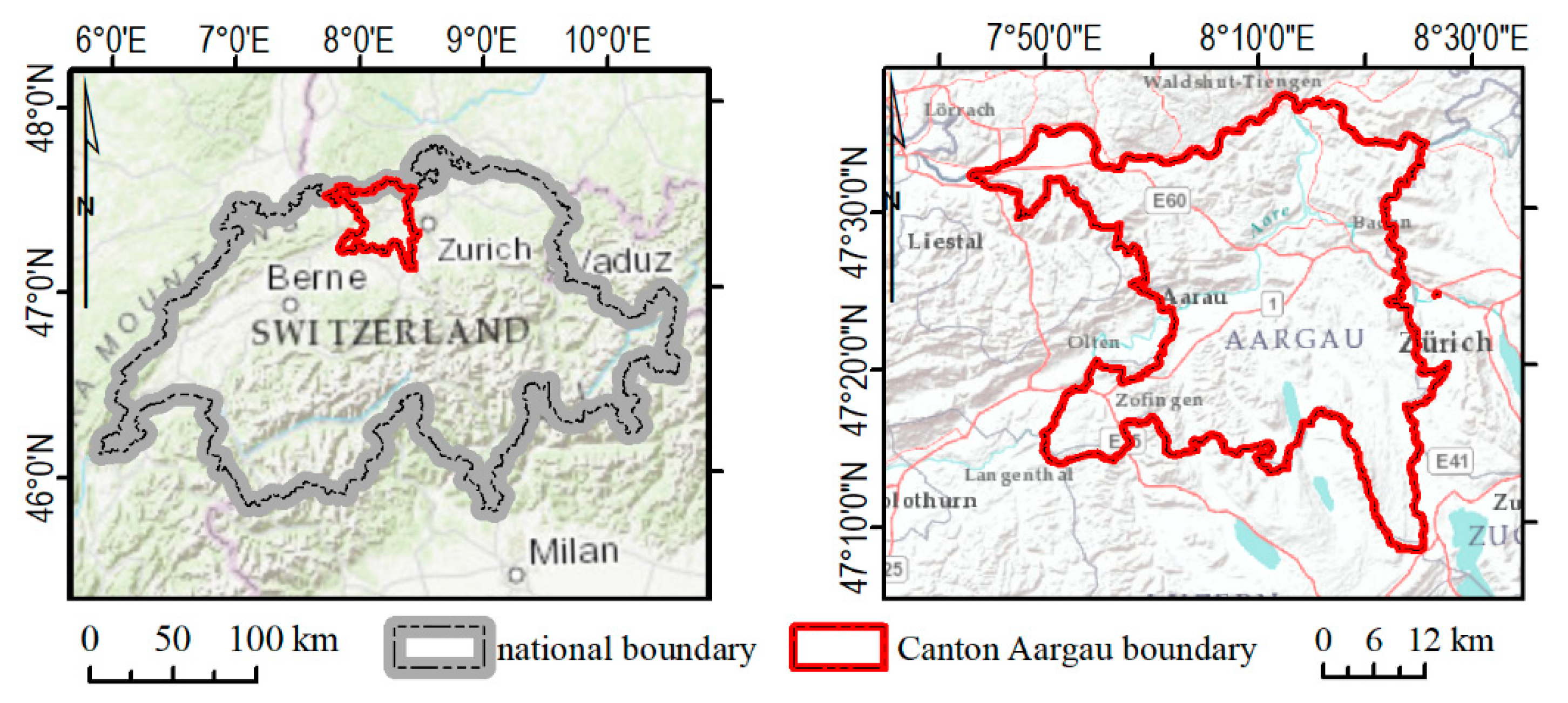
Switzerland is a central European country with 35.8% of its land area in agricultural usage, including 12.4% alpine agricultural areas. Grasslands constitute 70.3% of the agricultural area (UAA) [18]. However, the frequency of grassland mowing and the spatial distribution of different grassland and pasture management types across the country are not well known. Our study area is Canton Aargau (1403 km2), located within the Swiss Plateau (Figure 1), an undulating region with elevation ranging from 300 to 800 m a.s.l., and slopes reaching 55°. Almost 50% of the Canton is under agricultural land use. With some of the most fertile farmland in Switzerland, relatively large areas are managed intensively. The average farm size is 20.8 ha. More than half of the agricultural area is meadows or pastures (53%), and most of the rest is cropland (with main cultivation being maize, wheat, barley, potatoes, sugar beets, and rape) (Swiss Statistics, www.bfs.admin.ch). On the most intensively used grasslands, the first mowing event generally takes place in April, while on extensive grasslands the date of first mowing is later and depends largely on whether the land qualifies for direct payments [5]. Fields that are subject to subsidies cannot be mown in this region earlier than 15 June, and often the grass is cut just after this date.
2.2. Data
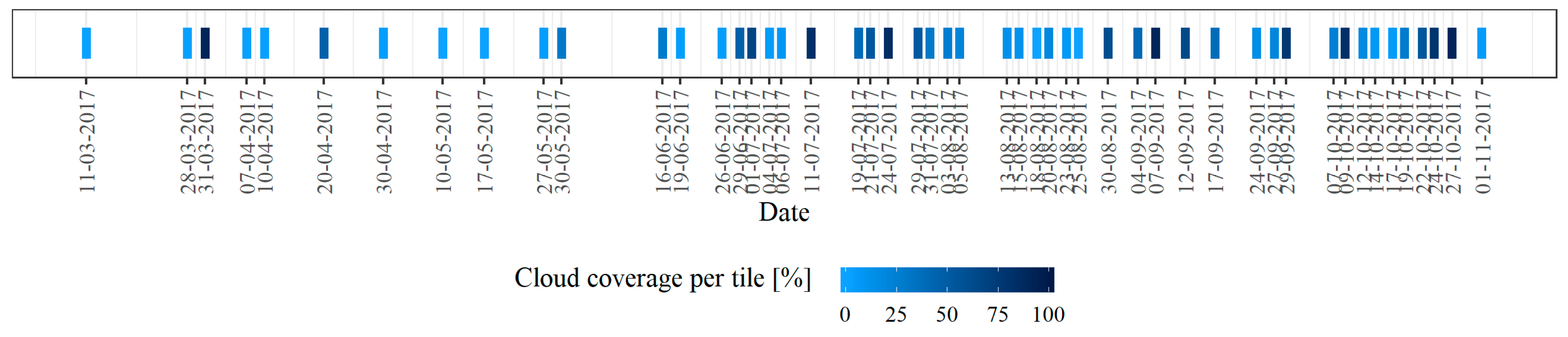
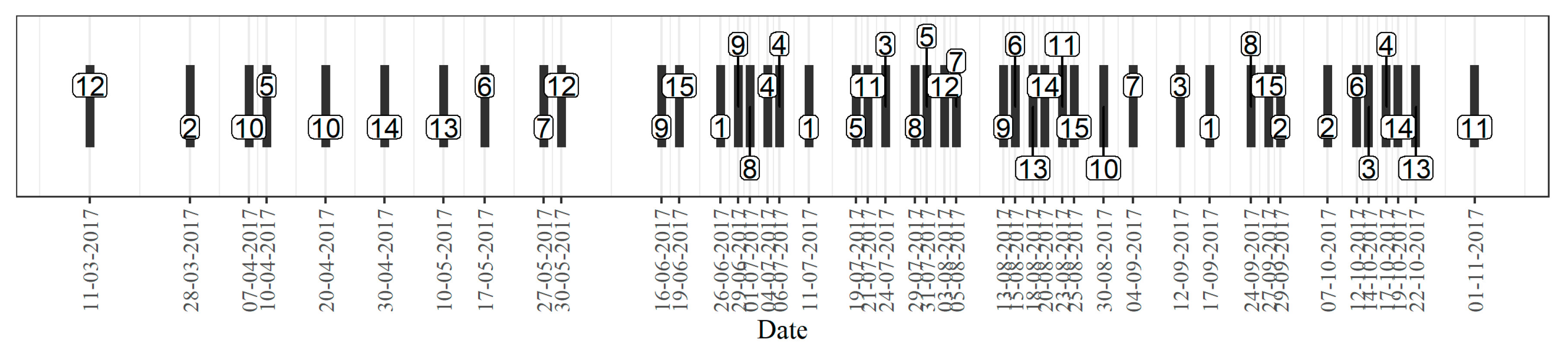
We downloaded S2 Level-1C images, tile identifier 32 TMT, captured between 1 March 2017 and 1 November 2017, with ESA-reported cloud cover less than 95% per tile. The Level-1C product contains a projected and ortho-rectified image expressed in Top Of Atmosphere (TOA) reflectance, as well as a cloud mask processed with data sampled at 60 m spatial resolution and resampled to 10 m and 20 m [10,19]. The downloaded dataset included 50 images distributed irregularly over the investigated period (Figure 2).
Auxiliary data included: (i) Land cover vector layers from the Swiss Federal Office of Topography’s (swisstopo) Topographic Landscape Model Model (TLM) and the Swiss national vector map 1:25,000 (VECTOR25). This dataset details forest, water, wetlands, rocks, and glacier coverage, updated within 2010–2016 (TLM Landcover), and built-up area, updated during 1987–2006 (VECTOR25 Primary surfaces). (ii) A vector layer with parcel boundaries and information on agricultural land use in 2017, sourced from land holders via the cantonal authority. The grassland categories included three subcategories, namely Artificial Meadows (fields in crop rotation, currently used for grass production), Permanent Meadows, and Permanent Pastures, divided into specific grassland types (Table S1). Parcel polygons that were not larger than 1000 m2 (10 pixels) were initially eliminated as potentially error-prone due to being covered mostly by mixed use pixels. The remaining parcels were then shrunk by 10 m to avoid mixed pixels at parcel edges, referred to as edge effect. The datasets included 71,252 non-shrunken and 62,420 shrunken parcels, referred to as parcels and shrunken parcels, respectively.
2.3. Methods
This study aims to investigate the potential of S2 imagery for mapping mowing frequency and develop an optimized processing approach for this purpose. The temporal phenological profiles of various agricultural land use types were constructed and analyzed using the NDVI which is generated from red and near-infrared spectral bands at 10 m spatial resolution. NDVI is one of the most widely used vegetation indices in vegetation-related studies [20,21], mainly because it is effective in limiting spectral noise arising from topography, cloud shadows and illumination conditions [22].
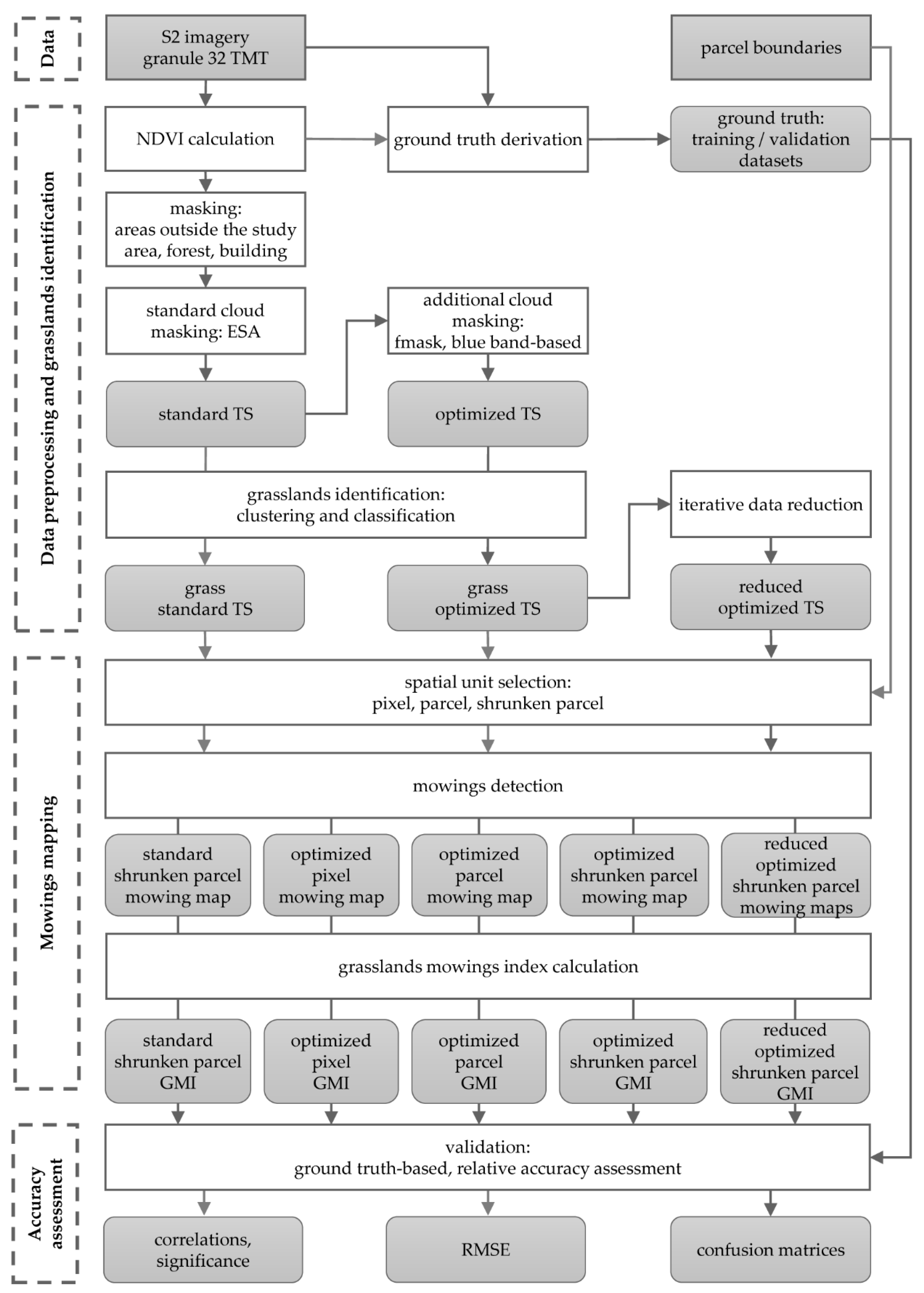
In general, gentle periodic NDVI increases and decreases over a season reflect the natural growth and decay of vegetation, while abrupt drops of the index indicate agricultural activities such as grass mowing, fertilization or crop harvesting. Our aim was to detect and count sudden drops of NDVI on grasslands that are related to mowing events. The proposed strategy involved four basic steps: (i) data preprocessing and land use/land cover classification into “grass” and “non-grass”; (ii) ground truth data derivation; (iii) mowing detection for grasslands management mapping; and (iv) validation/evaluation, for assessing accuracy of mowing events detection, and comparison of the results derived from various different analysis approaches. Step iv was repeated for two different cloud masking approaches and three different spatial mapping units, namely pixels, parcel polygons and shrunken parcel polygons (Figure 3).
2.3.1. Data Preprocessing and Grassland Identification
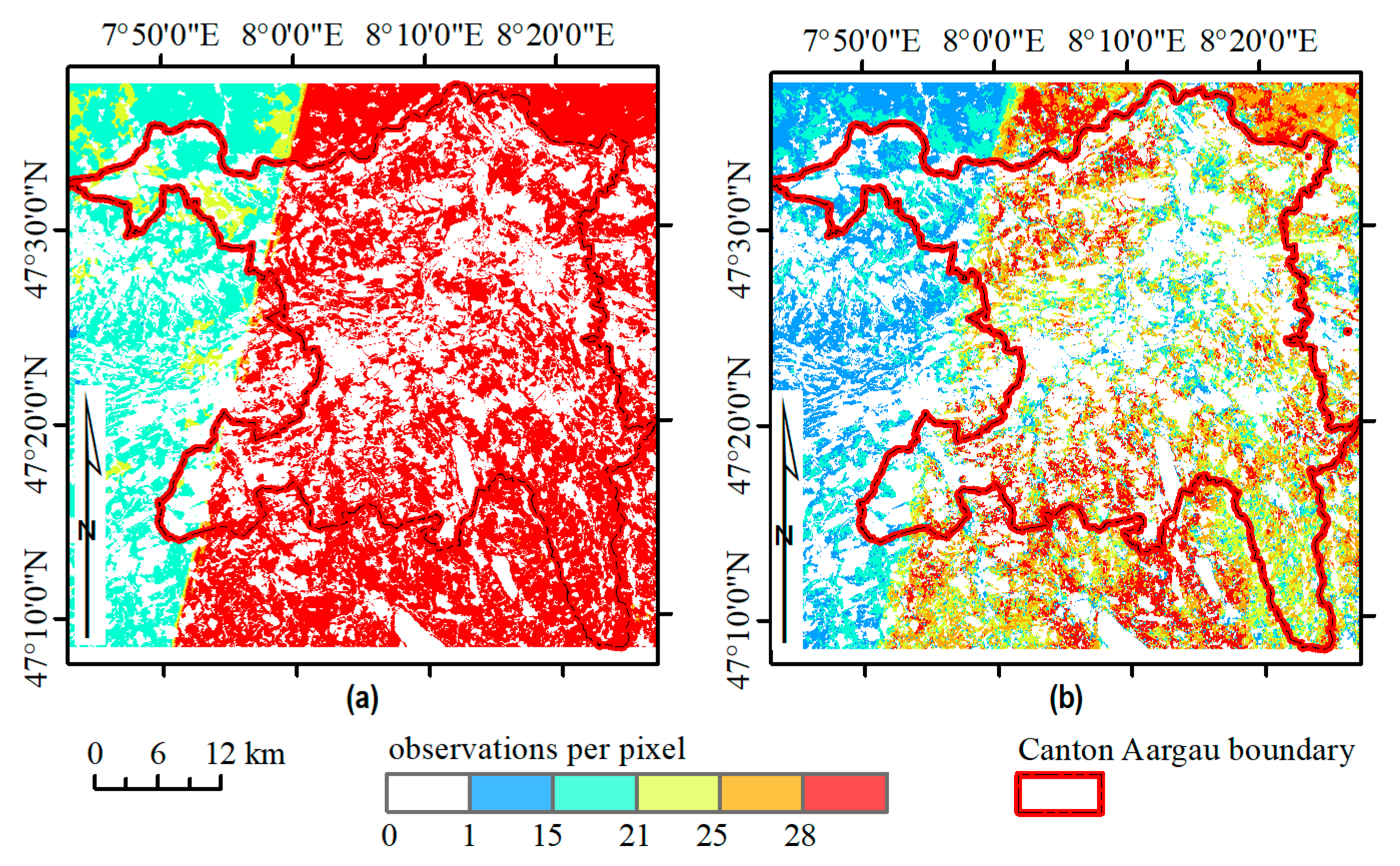
We used S2 Level-1C imagery, with no additional atmospheric and geometric corrections applied. Preprocessing of the S2 imagery included several steps. First, NDVI was calculated. Second, the data were clipped to the boundary of Canton Aargau enlarged by a 50 m buffer. Third, forest and built-up areas were masked using the topographic vector data. Fourth, the ESA opaque and cirrus cloud masks were applied. Fifth, a raster stack was constructed of all available NDVI images. This raw raster stack, referred to as standard TS, had a maximum of 46 observations per pixel. It is worth noting that, due to the S2 image acquisition strip edge, the eastern side of the study area had a denser time series than the eastern part.
Despite the ESA declarations [23], many remaining clouds were observed after cloud mask application, as well as snow, which could significantly influence the analysis. Thus, an additional masking was applied to remove these artifacts using the Fmask algorithm [24], and a blue band-based mask. The blue band-based masking approach was built upon the findings of Breon and Colzy (1999) and Hagolle et al. (2015) [25,26], who reported high cloud and snow reflectance in the blue spectrum (the same is true for some buildings and artificial surfaces, but these were already removed in the previous land use masking step), higher for low and opaque clouds than for high and thin clouds. We performed many tests using blue (S2 band 2) channel thresholding to find an optimal break value to mask as much cloud and snow as possible, but not influence bright surfaces. The tests were performed in Google Earth Engine for efficiency reasons. Based on visual assessment, we found the dimensionless (dl) reflectance threshold value of 1500 in band 2 suitable for masking as not only opaque clouds, but also most thin clouds were removed. Then, the blue band-based mask was produced in few simple steps: blue band (S2 band 2) thresholding at 1500 dl pixel values, buffering by 5 pixels to include haze at the borders of clouds, and masking holes smaller than 100 pixels. This additional masking resulted in an optimized time series, with maximum of 37 observations per pixel over the length of the time series (Figure 4).
Pixel-based land cover classification was performed to distinguish grassland parcels and parcels of other land uses that were excluded from further analysis. We did not use the cantonal agricultural land use data in this step as it is not available for many other regions, and transferability of the method is of high importance. The classification was conducted independently for the standard and optimized TS. For detection of grassland areas, we first applied a linear imputation of missing values for irregular time series (R package zoo and na.locf function) for the spatial location of each pixel. Then, we performed k-means clustering of the pixel time series with 12 clusters and 50 different random starting assignments. The optimal number of clusters was found using the elbow method, which considers the percentage of variance explained as a function of the number of clusters: a final number of clusters is found when adding another cluster does not significantly increase the variance explained [27]. To reduce the salt and pepper effect on the resulting cluster map, we applied a focal majority filter with a 3 × 3 pixel window size. Differentiation of grass and non-grass clusters was aided by careful visual inspection against the orthophoto map and visual comparison of the NDVI profiles of clusters and the agricultural land use data. Non-grass pixels were then masked out from the respective NDVI time series. The data were then aggregated to the parcel level, whereby parcels containing more than 50% grass pixels were considered grasslands. We characterized correspondence between grass/non-grass classification and the ground data using a confusion matrix [28] (Table S2).
2.3.2. Training and Validation Data
The training and validation data were necessary for mowing events detection methodology development (Section 2.3.3) and accuracy assessment (Section 2.3.4). The samples were derived manually as reference data including exact mowing dates for particular parcels were not available (not collected by Canton Aargau). We subset the available image times series into areas with the highest number of available observations (min = 30) and manually identified grassland parcels of homogeneous land use within these areas using red, green and blue (RGB) image composites assisted by knowledge of the general patterns of grassland management in the study area. We randomly sampled 70 grassland parcels and generated the NDVI profiles over the season. Based on the RGB composites and NDVI profiles we manually derived mowing frequency and dates. The dataset was split into training and validation samples of 20 and 50 parcels, respectively. Within the validation set we observed 125 mowing events between 20 April and 7 October 2017.
2.3.3. Grass Mowing Index
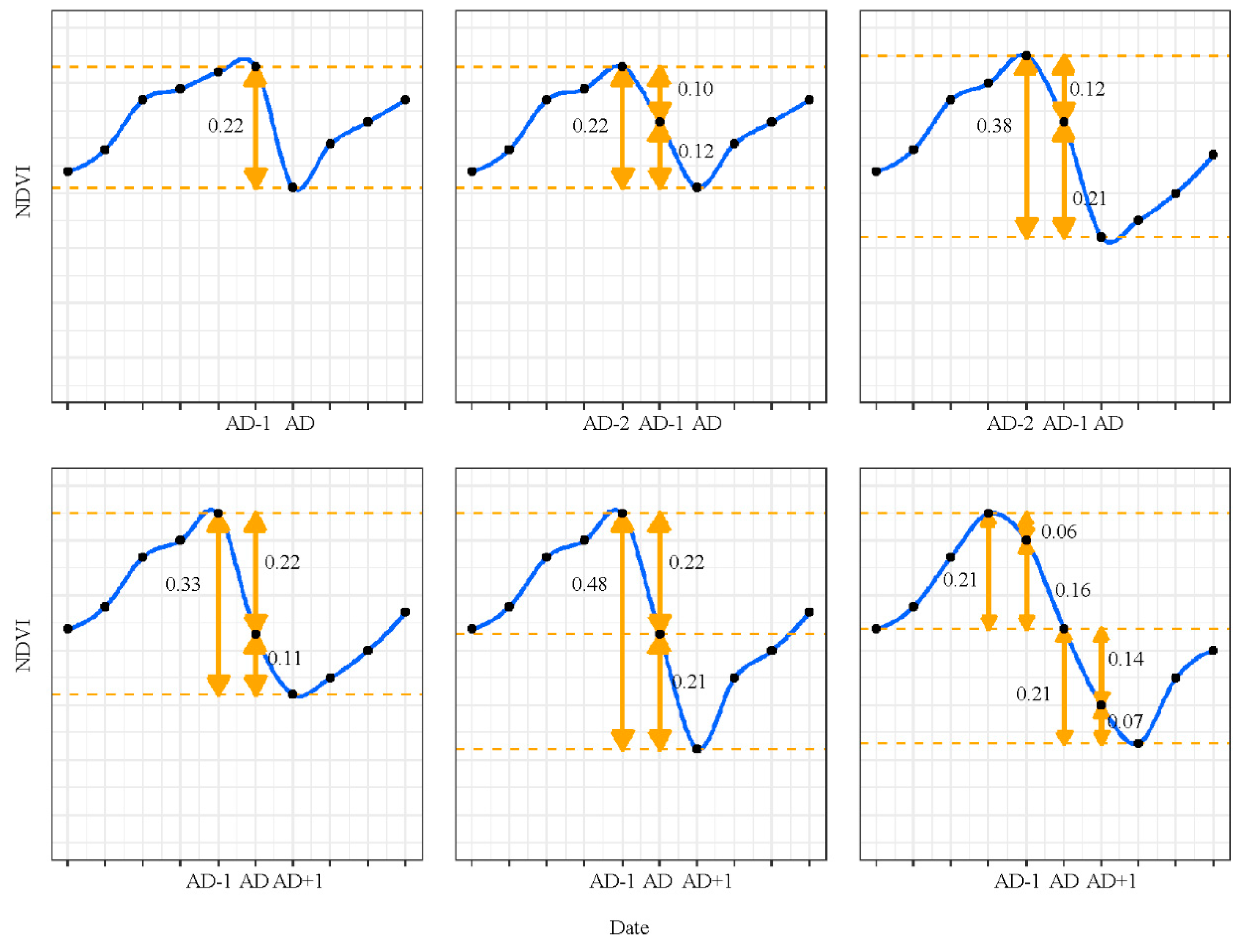
To develop a rule set for detection of mowing events, we first determined the general observed NDVI profiles for grasslands in Canton Aargau using the training sample. Grasslands in Canton Aargau were found to have relatively high NDVI values at the beginning of March, increasing gently until the first mowing. NDVI of bare ground did not exceed 0.3, while for high grass NDVI values were typically larger than 0.65. Following mowing NDVI dropped by at least 0.2, and recovered half of the drop within 8–10 days. If grass was mown, but not removed before the next image acquisition, the NDVI was observed to still be relatively high (drop of 0.05–0.10). Then, the next image acquired after the grass removal showed NDVI values typical for mown grassland (drop of at least 0.2 compared to the before-mowing values).
Based on these observations we developed a ruleset for mowing event detection. We defined a valid observation as a clear Sentinel-2 observation (pixel or parcel based) at a given acquisition date (AD). Observation gaps were not filled. For each AD, we extracted the following values:
- NDVI value.
- NDVI difference between AD and proceeding clear observation AD-1.
- NDVI difference between AD and the second-to-last clear observation AD-2.
- Day of the year of the AD.
- Number of days between AD and proceeding clear observation AD-1.
- Number of days between AD and the second-to-last clear observation AD-2.
To identify the number and dates of mowing events, we searched for NDVI drops of more than 0.2: (i) between consecutive clear observations; and (ii) between the current and the second-to-last clear observations. We checked for and excluded overlapping events (mowing events indicated by both conditions at the same date or at subsequent dates), prioritizing mowing detected by the first condition. Mowing events were assigned to the AD that was the first observation after the management event (Figure 5). We produced maps of number of detected mowings and day of the year of the first mowing.
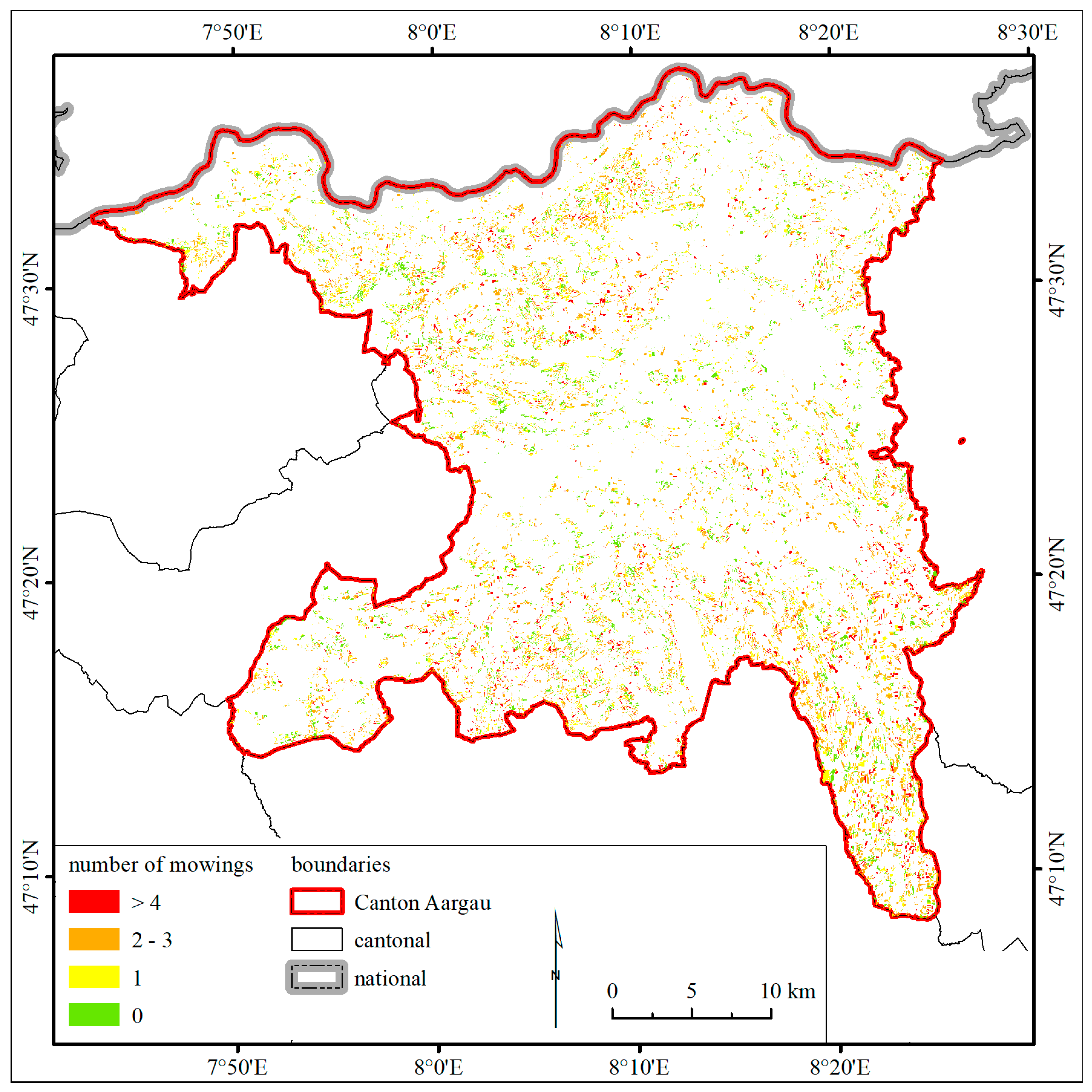
To summarize mowing frequency and schedule, we developed the grasslands mowing index (GMI), considering the Swiss regulations on the date of first mowing. First, grasslands mown 0, 1, 2–3 or >3 times were classified as not mown, low, medium and high mowing frequency, respectively. Second, the mown grasslands with first mowing event before or after 15 June were classified as early and late, respectively. Late mown grasslands are regarded as more extensively used than early mown [5]. We ranked the seven categories by ascending use intensity: not mown, low-late, medium-late, high-late, low-early, medium-early, and high-early. Areas of non-grass use were assigned NA. We checked how the GMI corresponded to observed agricultural land use and if this and mowing frequency were related to parcel size, tree fraction, mean elevation and mean slope. The tree fraction was calculated based on the vegetation height model from the Swiss National Forest Inventory [29], as the proportion of parcel area covered by vegetation higher than 3 m. Mean elevation and mean slope were calculated using the digital elevation model at scale 1:25,000 (DEM25) [30].
To investigate the potential of S2 for the detection of grass mowing, three spatial mapping units were tested: grassland pixels, grassland parcels and shrunken grassland parcels. The observations were NDVI values for pixels, and median NDVI for parcels. Considering the standard and optimized time series (various levels of clouds masking), and the three mapping units, we undertook the following experiments: (i) optimized-pixel; (ii) optimized-parcel; (iii) optimized-shrunken-parcel; (iv) standard-shrunken-parcel; and (v) iteratively reduced optimized-shrunken-parcel (based on reduction of input imagery). Optimized-pixel results were then aggregated to parcel and shrunken parcel to enable comparison between various approaches. Case (v) artificially simulated missing images to investigate the implications of missing imagery (for example due to cloud cover) for the mowing detection results. We set initial conditions as parcels with at least 30 available NDVI images and an area larger than 1000 m2. This resulted in a sample of 1345 shrunken parcels. In each of 15 iterations, three randomly chosen images were removed until only five images remained (Figure 6). For the standard TS, we analyzed only shrunken parcels to eliminate edge effect, that is mixed pixels at parcel edges, and focus exclusively on the influence of clouds.
2.3.4. Accuracy Assessment
We performed a two-stage accuracy assessment. First, we used the manually derived validation dataset to evaluate the accuracy of mowing event detection for each of Experiments (1)–(4) in terms of correlation (r) and significance value (p-value) supported by root mean square error (RMSE). Results from the pixel-based analysis (Experiment (1)) were aggregated to parcels and shrunken parcels using a majority rule. Second, the results with the highest correlation and lowest p-value, and confirmed by low RMSE, were treated as a reference for comparison with the number of mowings and date of first mowing obtained from the remaining experiments. The relative accuracy was assessed in terms of overall accuracy, producer’s accuracy, and user’s accuracy metrics [28] using the datasets containing all parcels. Within Experiment (5), the results of each iteration were compared to the reference experiment results with respect to the number of detected mowings and the number of mowings detected at the same date.
We checked if differences in number of mowings between the reference experiment and all the other experiments were correlated with parcel characteristics such as parcel size, tree fraction, mean elevation and mean slope.
3. Results
3.1. Data Preprocessing
Differentiation of grass and non-grass pixels was based on interpretation of the phenological profiles of clusters. The profiles based on the optimized TS are smoother than profiles based on standard TS (Figure S1), but the general patterns correspond well to each other. In general, four types of profiles can be distinguished: (i) flat profiles where low values of NDVI represent buildings and artificial surfaces; (ii) sinusoidal profiles including both very low and very high values of NDVI representing various crop types; (iii) gentle profiles rising at the beginning and descending at the end of the growing season but with NDVI remaining slightly above 0.5 representing single trees, groups of trees, and tree lines; and (iv) grassland represented by gently fluctuating profiles of values rarely below 0.5 but higher than in Type (3). This categorization of profiles was confirmed by comparison to NDVI profiles of reference land use categories using a pixel-based cross tabulation (Figure S2).
Comparing the profile categories to the results of the k-means clustering, we selected two grass clusters for the standard TS, and two clusters for the optimized TS, which indicated grass areas of 223.65 km2 and 247.15 km2, respectively. The area of parcels classified as grasslands equaled to 236.49 km2, 230.06 km2, and 207.16 km2, for classifications of optimized-shrunken-parcel, optimized-parcel and standard-shrunken-parcel, respectively. The number of grassland parcels exceeded 20,000 for each of the classifications, and 19,125 of them were classified as grasslands in all cases.
3.2. Grass Mowing Index
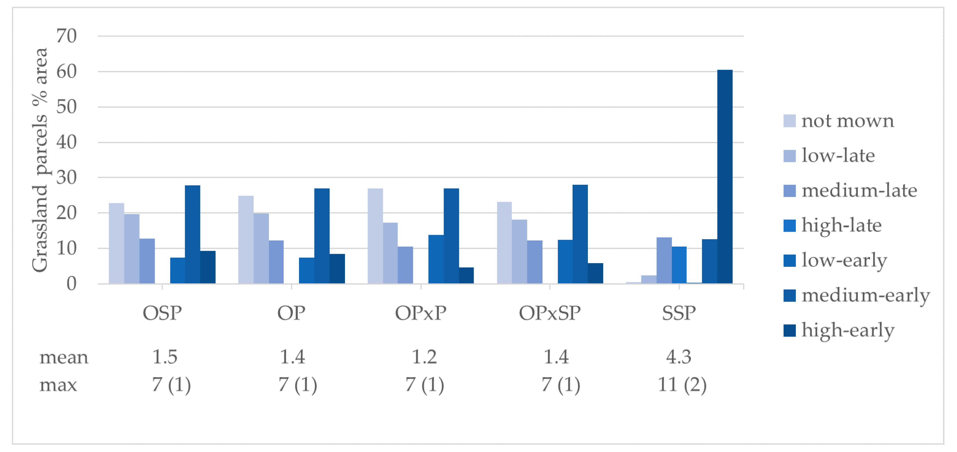
The results based on the optimized TS were consistent with one another, while, in comparison, the standard TS significantly overestimated number of mowings (Table S3 and Figure 7, Figure 8 and Figure 9). According to the optimized TS, 22.8–27.0% of grassland parcels area were not mown at all, 42.8–46.3% were mown early, and 27.8–32.7% were mown late, but the numbers of parcels mown early and late were equal. Larger parcels were mown early more frequently than small parcels. The standard TS identified 0.5% of parcels not mown, and almost 75% mown early. The optimized and standard TS showed, respectively, up to seven and eleven mowings per season, and the most frequent number of mowings equal to one and four or more. In both cases, fields of higher mowing frequency were rare.
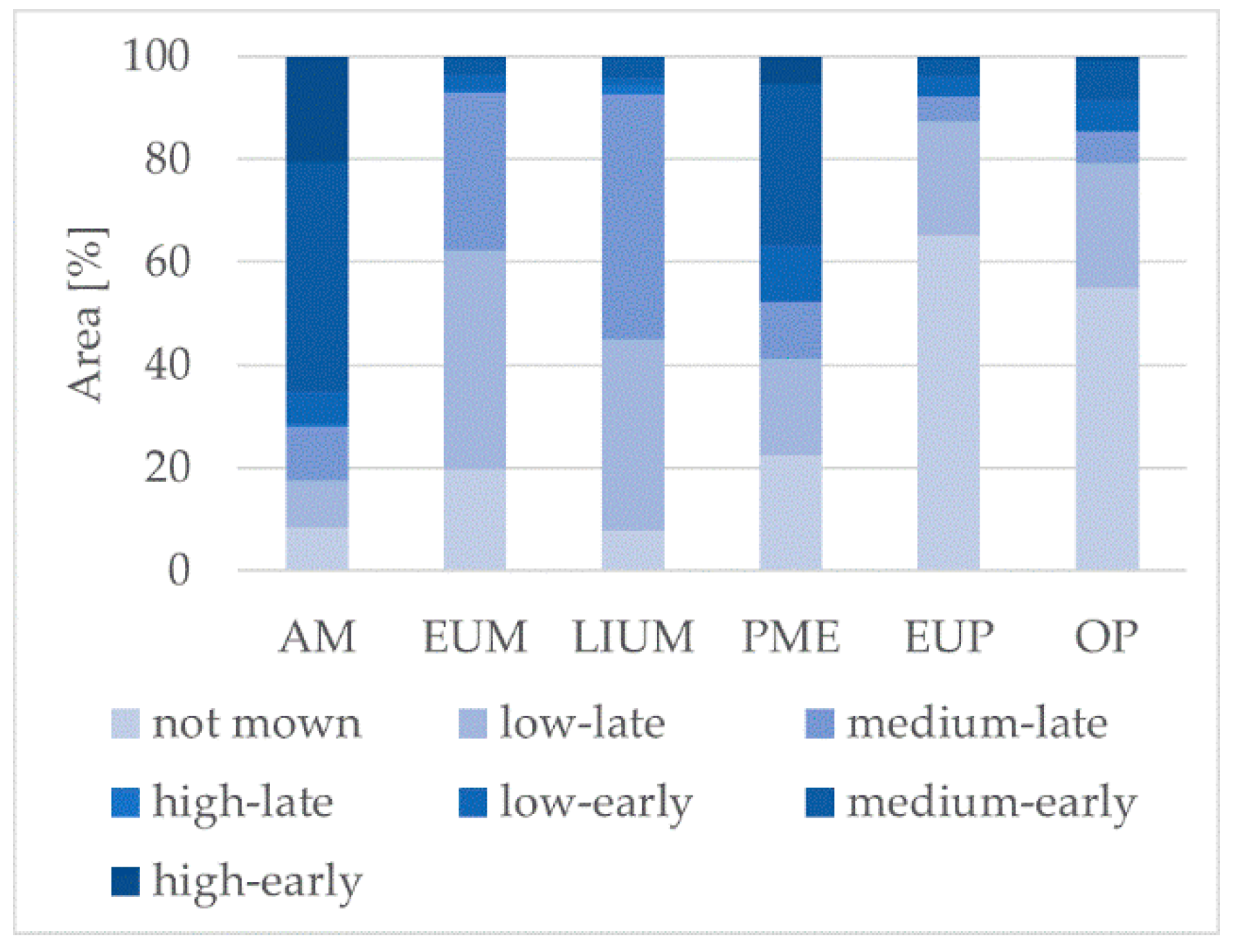
The classification of grassland area into the categories of the grasslands mowing index are similar across all the analyses based on the optimized TS (Figure 9 and Table S4). The highest GMI values were for artificial meadows, which were mown many times in the season, with the first cut taking place before 15 June. Extensively used pastures and other pastures have the lowest GMI values, as they were mown rarely and late in most cases. Extensively and less intensively used meadows were both mown late, but the former were mown fewer times. The largest variety of management was observed on permanent meadows, from no to many mowings, with the first mowing either early or late. The results for the GMI were substantially different for the standard TS analysis. All but one of the grassland categories were assigned the GMI category high-early, only extensively used pastures were mainly labeled as medium-late (Table S4).
According to parcel characteristics (Figure 10, Table 2), artificial meadows were located on the largest and mostly flat parcels with lowest tree fraction. Permanent meadows and pastures at the borders of farms were of medium size, on low to moderate slopes and with higher tree fraction. Extensively and less intensively used meadows both occupied the smallest parcels with moderate slopes and tree fraction. Extensively used pastures were located on medium size, steep parcels with the highest tree fraction. We found moderate negative correlation between mowing frequency and tree fraction (−0.24) and slope (−0.20), and weak positive correlations with parcel size (0.13) and elevation (0.06), all significant.
3.3. Accuracy Assessment
The accuracy assessment (using 125 observations of the validation dataset) indicated that the highest correlation coefficient (0.723), the lowest p-value (0.30 × 10⁻⁸), the second lowest RMSE (1.058), and correct detection of high number of mowing events was associated with the optimized-shrunken-parcel approach (Table 3). The optimized-pixel aggregated to shrunken parcel approach showed slightly worse correlation and p-value (0.718 and 0.45 × 10⁻⁸, respectively) and the lowest RMSE (1.039). All the results based on the optimized TS showed a strong positive relationship with the validation dataset, but the relationship was more significant for shrunken-parcel-based than parcel-based approaches. The lowest correlation, and highest p-value and RMSE were obtained using the standard-shrunken-parcel approach. Although this approach had the highest number of correctly detected mowing events, it also falsely identified a very high number of mowing events. Visual inspection of the results revealed overestimation of mowing events for optimized and standard time series was likely due to fertilization events or remaining clouds, respectively, which can cause a similar drop in NDVI as mowing.
Relative accuracy was used to evaluate the entire dataset against the reference experiment (optimized-shrunken-parcel). The greatest similarity to the reference results was found with the optimized-parcel approach with user’s and producer’s accuracies higher than 73% (Table S4). Investigation of NDVI profiles for individual parcels confirmed high similarity between the optimized-shrunken-parcels and optimized-parcels, and large discrepancies between those and standard-shrunken-parcels.
In most cases, correlations between differences in numbers of detected mowing events and parcel area, tree fraction, mean elevation and mean slope were very weak but significant (Table S5). Optimized-pixels aggregated to parcels were not correlated with mean elevation, and optimized-pixels aggregated to shrunken parcels showed no correlation to parcel area. All other variables showed very weak but significant correlations to differences in numbers of detected mowing events. The only positive correlations were for differences between Experiment (3) and Experiment (2) results and tree fraction, mean elevation and mean slope.
3.4. Imagery Reduction
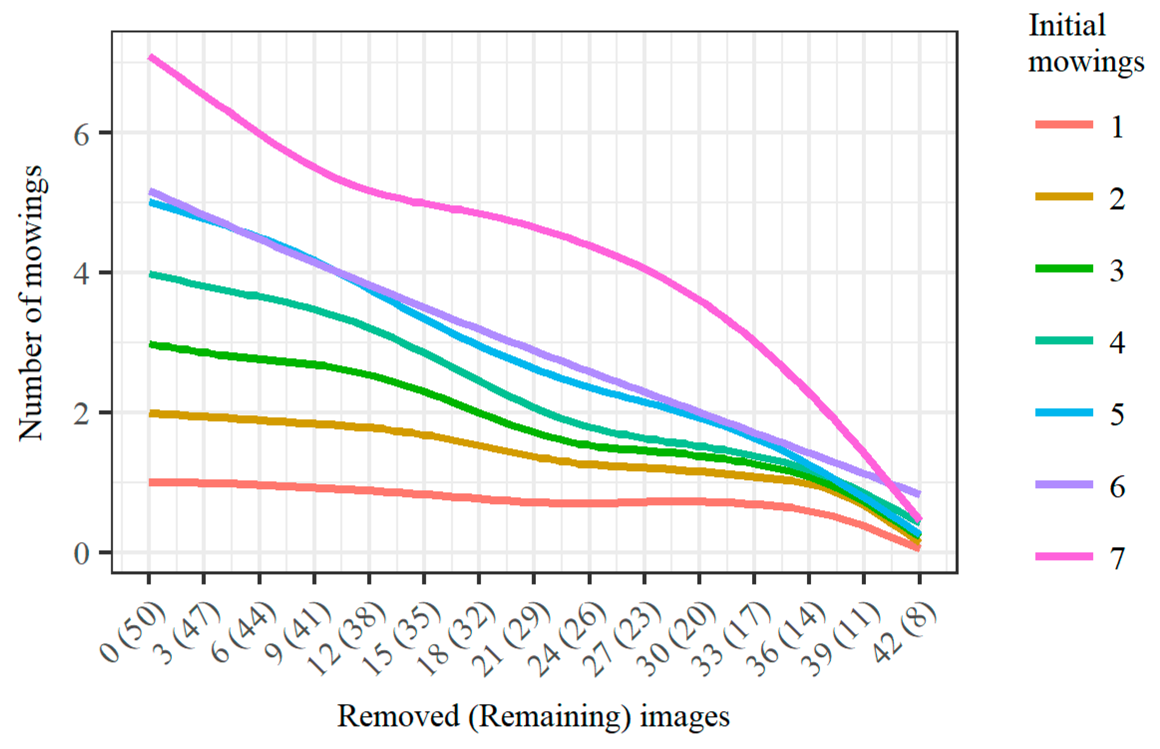
The overall tendency was that with decreasing number of input images, fewer mowing events are detected, or they are detected at different dates. Parcels with high frequency of mowing were more sensitive to image removal than those with low frequency of mowing (Figure 11). A significant shift in number of mowing events detected at the same date was observed after removal of 15 images of the total of 50 images, and after removal of 18 images there was less than 25% matches (Figures S3 and S4). This also holds for the one-time mowing events that are little affected by the reduction of images.
4. Discussion
This study investigated the performance of S2 time series for detection of grass mowing events. The data were shown to be effective in detecting spatial differences in grass mowing over large areas. Various GMI values show that, while on some plots farmers make intensive use of their land, in other parts of the study region grassland is managed less intensively in ways that can be considered to be maintaining biodiversity (Table 3). When using occurrence and date of first mowing as an indicator of grasslands use intensity, as did Franke et al. and Gomez et al. [2,8], we learn that slightly more grasslands are used extensively than intensively, inclusive of not mown land. Quite a high proportion of the unmown parcels may be fields used as grazing pastures, as grazing causes only subtle NDVI changes. Grassland use intensity is to some extent regulated by environmental conditions (Table 3). Large, flat and non-wooded plots of land are favorable to machinery operations and distribution of fertilizers. They are easily accessible and more efficient to manage than fragmented, steep or overgrown parcels. Thus, they are often used more intensively, especially for hay and fodder production or are a part of crop rotation areas subject to a regular application of nutrients. On the other hand, the less accessible parcels promote biodiversity through reduction of environmental impacts on meadows or pastures.
We managed to discriminate between various frequencies and dates of mowing. As expected, clouds and mixed pixels decreased the accuracy of mowing detection. The most accurate results were obtained for optimized-shrunken-parcel analysis, where the influence of the two constraints was reduced (Table 3). Validation showed that we correctly detected 96 out of 125 (77%) mowing events, but we also detected nine mowing events that did not occur. These falsely detected events can largely be explained by field fertilization, which is another important indicator of grassland use intensity. Analysis based on various spatial mapping units: pixels, parcels and shrunken parcels, produced similar results. The results also suggested a smoothing effect of field edges, possibly due to neighboring land uses of more constant or lower NDVI, e.g., trees or artificial surfaces. However, the edge effect was not very clear, which may be due to most non-grass-covered areas being eliminated prior to mowing detection. While clustering allowed removal of non-grass pixels (e.g., trees) from the inside and the edges of parcels and single pixels with erroneous spectral reflectance, parcel shrinking removed only remaining edge pixels that were mostly grass, and thus did not cause much change to the results.
Using either parcels or shrunken-parcels as spatial units for mowing detection was difficult when different management practices occurred on a single parcel (e.g., temporal fallow plot on a part of the actively used parcel), were partly shaded by forest and trees or included terrain shadows not corrected in the imagery. A possible method to overcome this issue is an object-based approach [31] which segments an area into spectrally homogeneous and spatially related units with limited influence of noisy pixels. This approach can be used to detect patches of different phenology within existing parcels or within the entire area if parcel boundaries are not available [32]. However, in the case of high variation in field size within the study area, a particular scale parameter that is suitable in one place can lead to over- or under-segmentation in another location [15]. Therefore, as Canton Aargau contained parcels of area ranging from 0.1 ha to 30 ha, we decided to perform a pixel-based classification.
We found careful cloud masking critical for correct identification of grassland mowing events for two reasons. First, the single-date cloudy observations cause a sudden drop of NDVI that can be easily confused with mowing events and lead to overestimation of their number. Second, long cloudy periods preclude detection of rapid and irregular events, such as grass mowing. This occurs because in favorable conditions (humidity, temperature) grass can regrow rapidly, with NDVI returning to pre-mowing levels within a week. Thus, even weekly cloudy periods may preclude detection of some mowing events. Our imagery reduction experiment confirmed that more frequent observations result in better coincidence with key events in the grass growth season and detection of single agricultural activities, and not only characterization of general trends in grasslands use intensity [2,8].
Obtaining a dense cloud free time series is thus the biggest challenge for detection of grass mowing, and is very location dependent [33]. In the Swiss Plateau, the climatic conditions limit the number of cloud-free days as this is the least sunny region in Switzerland with an average of more than ten rainy days per month. Only 50 of 67 available images captured between 1 March 2017 and 1 November 2017 for Canton Aargau had ESA defined cloud cover less than 95%, with an average of 31%. In most cases, the real cloud cover was higher, so the number of usable (cloud-free) scenes was much lower. We found that neither the ESA cloud mask nor Fmask could handle both dense and cirrus clouds. Thus, we applied a blue band-based algorithm that allowed removal of most clouds. This method had advantages over other existing solutions. It did not lead to over-reduction of available clear observations, which is often the case with generation of cloud free, seasonally and radiometrically consistent periodic mosaics [17,33,34]. The blue band method was also less time-consuming than some ready-to-use algorithms [26,35]. The method may also remove bare soil or buildings, however this would not affect the results of grass mowing detection. Recent improvements to the S2 Fmask [36] may mean improved cloud detection and less need for the blue band approach, but this implementation was not available to us at the time of our research.
A very good user’s accuracy for grass classification ensured that other land use types were not included in the grass class and that the mowing event analysis dataset was almost entirely grass pixels. The relatively low producer’s accuracy can partially be explained in that the reference data described land use information, while the pixel-based classifications were for land cover. In particular, the differences might have arisen from the fact that some reference parcels: (i) were divided into smaller pieces of land each with different management; (ii) included other land cover elements such as trees; (iii) were partly shadowed by forest and trees; and (iv) were adjacent to roads causing mixed pixels. Much omission error could be caused by clusters containing trees, shadows and artificial surfaces being classified as non-grass, even if they overlapped the reference grasslands. Analogically, grass patches may occur on areas of another land use category, e.g., orchards, which would increase the commission error. Investigation of only grass pixels allowed limiting the edge effect in the case of parcel-based analysis. Therefore, we assume that the low producer’s accuracy of grass class had only a marginal impact on the mowing event detection results of our study.
We found the NDVI time series based method developed here powerful for mapping grass mowing frequency over various areas for two reasons. First, it is not conditional upon the availability of reference data, which is often missing, contrary to widely used machine learning strategies, which require training data. Understanding seasonal and phenological aspects of management practices in the study area was sufficient to allow discrimination between grass and non-grass clusters and, together with careful investigation of satellite imagery, allowed for development of a rule set for mowing event detection. Second, the method we developed can easily be transferred to different landscape types and management systems. There are two steps that require a discretionary decision: selection of grass clusters during land use classification, and setting a NDVI drop threshold to indicate a mowing event. Reference data can aid in determining land use types and their phenological profiles, especially for detailed crop species mapping, but is not necessary if the main goal is to distinguish between just two categories, namely grass and non-grass. In most European countries, the bare ground period (e.g., very low NDVI) is sufficient to eliminate non-grass areas [37]. While records including dates of grass mowing for a set of parcels would be helpful, guiding information can be successfully derived through visual interpretation of imagery.
This study is a proof of concept for using Sentinel-2 for grassland management mapping. A limitation of the approach is the sensor spatial resolution, which may be too coarse for imaging fragmented or long and narrow fields typical for rural landscapes in many mountainous areas [38,39], or unsuitable when a high level of detail is necessary to inform decisions at small spatial scales. In such cases, alternative sources, such as unmanned aerial vehicles could be used.
Continued acquisition of S2 in the coming years will allow construction of longer time series useful for detection of crop rotation areas and changes in land management. That information should improve classification of land use intensity, especially differentiation between permanent and temporal grasslands, and detection of land use shifts and transitions, e.g., land abandonment areas.
5. Conclusions
This study illustrated that S2 time series have potential for regional scale mapping of mowing frequency. However, frequent images and careful cloud masking are required. Additional cloud masking and elimination of mixed pixels allowed identification of 77% of mowing events, while standard cloud masking led to considerable overestimation of mowing events. Denser time series increased the likelihood of detection of rapid events, especially in the case of intensively used grasslands with a high number of mowings, and had higher coincidence with key events in the grass growth season. The findings are important because they show that detection of individual grass mowing events is possible with Sentinel-2 imagery [17], and that grassland management mapping is not limited by using only cloudless images so long as they are carefully selected and acquired in crucial moments of the growing season [2,8]. Moreover, the applied methodology is not conditional upon the availability of reference data, which is particularly important in areas with limited ancillary data. The method also requires few discretionary decisions, and can be easily applied to different landscape types and management systems. In the future, longer S2 time series would enable discrimination between permanent and temporary grasslands by investigation of multi-seasonal management regimes in particular fields. Overall, the straightforward methodology can easily be applied to grassland management mapping in various areas, and therefore can contribute to the optimization of land use intensity and the encouragement of biodiversity friendly farming.
Supplementary Materials
The following are available online at https://www.mdpi.com/2072-4292/10/8/1221/s1, Figure S1: Phenological profiles of the most frequent land use classes, according to agricultural land use data from the Canton Aargau: (a) classes 500 s; (b) classes 600 s; and (c) classes 700 s, Figure S2: Phenological profiles of clusters, derived from pixel-based k-means clustering of: (a) standard time series; and (b) optimized time series, Figure S3: Relative difference between number of mowings detected with full and reduced image dataset, grouped by number of initial mowings, Figure S4: Mowings detected on the same date with reduction of input image dataset, grouped by number of initial mowings, Table S1: Grassland types according to from Canton Aargau data on agricultural land use in 2017, Table S2: Accuracy of grasslands identification for pixel- and parcel-based classifications. For pixel-level accuracy assessment, only pixels overlapping the cantonal agricultural land use dataset were considered. Pixel-based results are given as number of pixels multiplied by 1000. Parcel-based results are given as number of parcels, Table S3: Relative accuracy of mowing detection: comparison of number of mowings between the reference experiment (optimized-shrunken-parcel) and the remaining experiments, Table S4: Correspondence between GMI categories and agricultural land use types for various analysis approaches. The marginal agricultural land use types were not included. AM, artificial meadows; EUM, extensively used meadows; LIUM, less intensively used meadows; PM, permanent meadows; EUP, extensively used pastures; OP, other pastures (pastures bordering on the farm), Table S5: Correlations between differences in numbers of mowing events (between the reference experiment (optimized-shrunken-parcel) and the remaining experiments) and selected environmental variables. Insignificant correlation p-values are italic. OSP, Optimized-shrunken-parcel; OP, Optimized-parcel; OPxP, Optimized-pixel—aggregated to parcel; OPxSP, Optimized-pixel—aggregated to shrunken parcel; SSP, Standard-shrunken-parcel.
Author Contributions
N.K., P.V. and C.G. conceived and designed the study; N.K. performed the data analysis and interpretation; P.V., C.G., R.P. and B.P. assisted in the data analysis and interpretation; and all authors reviewed and improved the overall manuscript.
Funding
This research received no external funding.
Acknowledgments
This research reported was supported by European Union’s Seventh Framework Programme ERC Grant Agreement No. 311819—GLOLAND. We would like to thank the Canton of Aargau for making the data available for agricultural use of 2017.
Conflicts of Interest
The authors declare no conflict of interest.
References
- Kuemmerle, T.; Levers, C.; Erb, K.; Estel, S.; Jepsen, M.R.; Müller, D.; Plutzar, C.; Stürck, J.; Verkerk, P.J.; Verburg, P.H.; et al. Hotspots of land use change in Europe. Environ. Res. Lett. 2016, 11, 1–14. [Google Scholar] [CrossRef]
- Franke, J.; Keuck, V.; Siegert, F. Assessment of grassland use intensity by remote sensing to support conservation schemes. J. Nat. Conserv. 2012, 20, 125–134. [Google Scholar] [CrossRef]
- Ali, I.; Cawkwell, F.; Dwyer, E.; Barrett, B.; Green, S. Satellite remote sensing of grasslands: From observation to management. J. Plant Ecol. 2016, 9, 649–671. [Google Scholar] [CrossRef]
- Huyghe, C.; De Vliegher, A.; van Gils, B.; Peeters, A. Grasslands and Herbivore Production in Europe and Effects of Common Policies; Editions Quae: Versailles, France, 2014; p. 287. [Google Scholar]
- FOAG. Swiss Agricultural Policy. Objectives, Tools, Prospects; Swiss Federal Office for Agriculture: Bern, Switzerland, 2004; Available online: https://www.cbd.int/financial/pes/swiss-pesagriculturalpolicy.pdf (accessed on 30 June 2018).
- Beaufoy, G.; Baldock, D.; Clark, J. The Nature of Farming: Low Intensity Farming Systems in Nine European Countries. 1994, p. 66. Available online: https://ieep.eu/publications/the-nature-of-farming-low-intensity-farming-systems-in-nine-european-countries (accessed on 30 June 2018).
- Nemecek, T.; Huguenin-Elie, O.; Dubois, D.; Gaillard, G.; Schaller, B.; Chervet, A. Life cycle assessment of Swiss farming systems: II. Extensive and intensive production. Agric. Syst. 2011, 104, 233–245. [Google Scholar] [CrossRef]
- Gómez Giménez, M.; de Jong, R.; Della Peruta, R.; Keller, A.; Schaepman, M.E. Determination of grassland use intensity based on multi-temporal remote sensing data and ecological indicators. Remote Sens. Environ. 2017, 198, 126–139. [Google Scholar] [CrossRef]
- Jakimow, B.; Griffiths, P.; van der Linden, S.; Hostert, P. Mapping pasture management in the Brazilian Amazon from dense Landsat time series. Remote Sens. Environ. 2017. [Google Scholar] [CrossRef]
- ESA European Space Agency—Missions—Sentinel-2. Available online: https://sentinel.esa.int/web/sentinel/missions/sentinel-2 (accessed on 30 June 2018).
- Immitzer, M.; Vuolo, F.; Atzberger, C. First experience with Sentinel-2 data for crop and tree species classifications in central Europe. Remote Sens. 2016, 8. [Google Scholar] [CrossRef]
- Korhonen, L.; Hadi; Packalen, P.; Rautiainen, M. Comparison of Sentinel-2 and Landsat 8 in the estimation of boreal forest canopy cover and leaf area index. Remote Sens. Environ. 2017, 195, 259–274. [Google Scholar] [CrossRef]
- Shoko, C.; Mutanga, O. Examining the strength of the newly-launched Sentinel 2 MSI sensor in detecting and discriminating subtle differences between C3 and C4 grass species. ISPRS J. Photogramm. Remote Sens. 2017, 129, 32–40. [Google Scholar] [CrossRef]
- Rujoiu-Mare, M.-R.; Olariu, B.; Mihai, B.-A.; Nistor, C.; Săvulescu, I. Land cover classification in Romanian Carpathians and Subcarpathians using multi-date Sentinel-2 remote sensing imagery. Eur. J. Remote Sens. 2017, 50, 496–508. [Google Scholar] [CrossRef] [Green Version]
- Belgiu, M.; Csillik, O. Sentinel-2 cropland mapping using pixel-based and object-based time-weighted dynamic time warping analysis. Remote Sens. Environ. 2017, 204, 509–523. [Google Scholar] [CrossRef]
- Lopes, M.; Fauvel, M.; Ouin, A.; Girard, S. Potential of Sentinel-2 and SPOT5 (Take5) time series for the estimation of grasslands biodiversity indices. In Proceedings of the 2017 9th International Workshop on the Analysis of Multitemporal Remote Sensing Images (MultiTemp), Brugge, Belgium, 27–29 June 2017; Volume 5. [Google Scholar]
- Griffiths, P.; Hostert, P. Integration of Sentinel-2 and Landsat Data for Phenological Characterization of Semi-Natural Vegetation; Boston University: Boston, MA, USA, 2017. [Google Scholar]
- FSO. Food and Agriculture—Pocket Statistics 2017; Federal Statistical Office: Neuchâtel, Switzerland, 2017; p. 36. [Google Scholar]
- ESA. European Space Agency—Products—Sentinel-2 MSI. Available online: https://sentinel.esa.int/web/sentinel/user-guides/sentinel-2-msi/product-types/level-1c (accessed on 30 June 2018).
- Liang, S.; Yang, C.; Yu, D.; Ma, W. Extracting multiple cropping index based on NDVI time series: A method integrating temporal and spatial information. In Proceedings of the 3rd International Conference on Agro-Geoinformatics, Agro-Geoinformatics, Beijing, China, 11–14 August 2014; pp. 1–5. [Google Scholar]
- Esch, T.; Metz, A.; Marconcini, M.; Keil, M. Differentiation of Crop Types and Grassland by Multi-scale Analysis of Seasonal Satellite Data. In Land Use and Land Cover Mapping in Europe. Remote Sensing and Digital Image Processing; Manakos, I., Braun, M., Eds.; Springer: Dordrecht, The Netherlands, 2014; Volume 18, pp. 329–339. ISBN 978-94-007-7968-6. [Google Scholar]
- Huete, A.; Didan, K.; Miura, T.; Rodriguez, E.P.; Gao, X.; Ferreira, L.G. Overview of the radiometric and biophysical performance of the MODIS vegetation indices. Remote Sens. Environ. 2002, 83, 195–213. [Google Scholar] [CrossRef]
- ESA. European Space Agency—Sentinel-2—Cloud Masks. Available online: https://sentinel.esa.int/web/sentinel/technical-guides/sentinel-2-msi/level-1c/cloud-masks (accessed on 30 June 2018).
- Zhu, Z.; Wang, S.; Woodcock, C.E. Improvement and expansion of the Fmask algorithm: Cloud, cloud shadow, and snow detection for Landsats 4-7, 8, and Sentinel 2 images. Remote Sens. Environ. 2015, 159, 269–277. [Google Scholar] [CrossRef]
- Breon, F.-M.; Colzy, S. Cloud Detection from the Spaceborne POLDER Instrument and Validation against Surface Synoptic Observations. J. Appl. Meteorol. 1999, 38, 777–785. [Google Scholar] [CrossRef]
- Hagolle, O.; Huc, M.; Pascual, D.V.; Dedieu, G. A multi-temporal and multi-spectral method to estimate aerosol optical thickness over land, for the atmospheric correction of FormoSat-2, LandSat, VENμS and Sentinel-2 images. Remote Sens. 2015, 7, 2668–2691. [Google Scholar] [CrossRef]
- Kaufman, L.; Rousseuw, P.J. Finding Groups in Data: An Introduction to Cluster Analysis; Wiley-Liss, Div John Wiley & Sons Inc.: New York, NY, USA, 1990; ISBN 0471878766. [Google Scholar]
- Congalton, R.G. A Review of Assessing the Accuracy of Classifications of Remotely Sensed Data. Remote Sens. Environ. 1991, 46, 35–46. [Google Scholar] [CrossRef]
- Ginzler, C.; Hobi, M.L. Countrywide Stereo-Image Matching for Updating Digital Surface Models in the Framework of the Swiss National Forest Inventory. Remote Sens. 2015, 7, 4343–4370. [Google Scholar] [CrossRef] [Green Version]
- Swisstopo. The Digital hEight Model of Switzerland DHM25. Available online: https://shop.swisstopo.admin.ch/en/products/height_models/dhm25 (accessed on 20 April 2018).
- Blaschke, T. Object based image analysis for remote sensing. ISPRS J. Photogramm. Remote Sens. 2010, 65, 2–16. [Google Scholar] [CrossRef]
- Yin, H.; Prishchepov, A.V.; Kuemmerle, T.; Bleyhl, B.; Buchner, J.; Radeloff, V.C. Mapping agricultural land abandonment using spatial and temporal segmentation of dense Landsat time series. Remote Sens. Environ. 2018, 210, 12–24. [Google Scholar] [CrossRef]
- White, J.C.; Wulder, M.A.; Hobart, G.W.; Luther, J.E.; Hermosilla, T.; Griffiths, P.; Coops, N.C.; Hall, R.J.; Hostert, P.; Dyk, A.; et al. Pixel-based image compositing for large-area dense time series applications and science. Can. J. Remote Sens. 2014, 40, 192–212. [Google Scholar] [CrossRef]
- Griffiths, P.; Van Der Linden, S.; Kuemmerle, T.; Hostert, P. A pixel-based landsat compositing algorithm for large area land cover mapping. IEEE J. Sel. Top. Appl. Earth Obs. Remote Sens. 2013, 6, 2088–2101. [Google Scholar] [CrossRef]
- Hollstein, A.; Segl, K.; Guanter, L.; Brell, M.; Enesco, M. Ready-to-use methods for the detection of clouds, cirrus, snow, shadow, water and clear sky pixels in Sentinel-2 MSI images. Remote Sens. 2016, 8, 666. [Google Scholar] [CrossRef]
- Frantz, D.; Haß, E.; Uhl, A.; Stoffels, J.; Hill, J. Improvement of the Fmask algorithm for Sentinel-2 images: Separating clouds from bright surfaces based on parallax effects. Remote Sens. Environ. 2018. [Google Scholar] [CrossRef]
- Gómez Giménez, M.; Della Peruta, R.; De Jong, R.; Keller, A.; Schaepman, M.E. Spatial Differentiation of Arable Land and Permanent Grassland to Improve a Land Management Model for Nutrient Balancing. IEEE J. Sel. Top. Appl. Earth Obs. Remote Sens. 2016, 9, 5655–5665. [Google Scholar] [CrossRef]
- Kolecka, N.; Kozak, J.; Kaim, D.; Dobosz, M.; Ostafin, K.; Ostapowicz, K.; Wężyk, P.; Price, B. Understanding farmland abandonment in the Polish Carpathians. Appl. Geogr. 2017, 88, 62–72. [Google Scholar] [CrossRef]
- Gellrich, M.; Baur, P.; Koch, B.; Zimmermann, N.E. Agricultural land abandonment and natural forest re-growth in the Swiss mountains: A spatially explicit economic analysis. Agric. Ecosyst. Environ. 2007, 118, 93–108. [Google Scholar] [CrossRef]
Figure 1.
Study area Canton Aargau located in the northern part of Switzerland.

Figure 2.
Temporal availability of the Sentinel-2 time series data used in this study. Colors indicate cloud coverage per tile.
Figure 2.
Temporal availability of the Sentinel-2 time series data used in this study. Colors indicate cloud coverage per tile.

Figure 3.
Workflow overview. Sentinel-2 (S2); normalized difference vegetation index (NDVI); European Space Agency (ESA); time series (TS); grasslands mowing index (GMI); root mean square error (RMSE).
Figure 3.
Workflow overview. Sentinel-2 (S2); normalized difference vegetation index (NDVI); European Space Agency (ESA); time series (TS); grasslands mowing index (GMI); root mean square error (RMSE).

Figure 4.
Number of observations per pixel in: (a) standard TS; and (b) optimized TS. The white areas were excluded from the analysis. The eastern part of the study area is covered by much denser time series, due to overlap between Sentinel-2 stripes.
Figure 4.
Number of observations per pixel in: (a) standard TS; and (b) optimized TS. The white areas were excluded from the analysis. The eastern part of the study area is covered by much denser time series, due to overlap between Sentinel-2 stripes.

Figure 5.
Graph showing illustrative profiles and mowings. The black dots represent available imagery. Mowing date is indicated as AD, however the exact event date is between AD-1 and AD. If mowings were detected in subsequent dates, only the first was considered.
Figure 5.
Graph showing illustrative profiles and mowings. The black dots represent available imagery. Mowing date is indicated as AD, however the exact event date is between AD-1 and AD. If mowings were detected in subsequent dates, only the first was considered.

Figure 6.
Images reduction. Numbers indicate iteration in which the image was removed.

Figure 7.
Mowing frequency map of Canton Aargau derived from optimized-shrunken-parcel.

Figure 8.
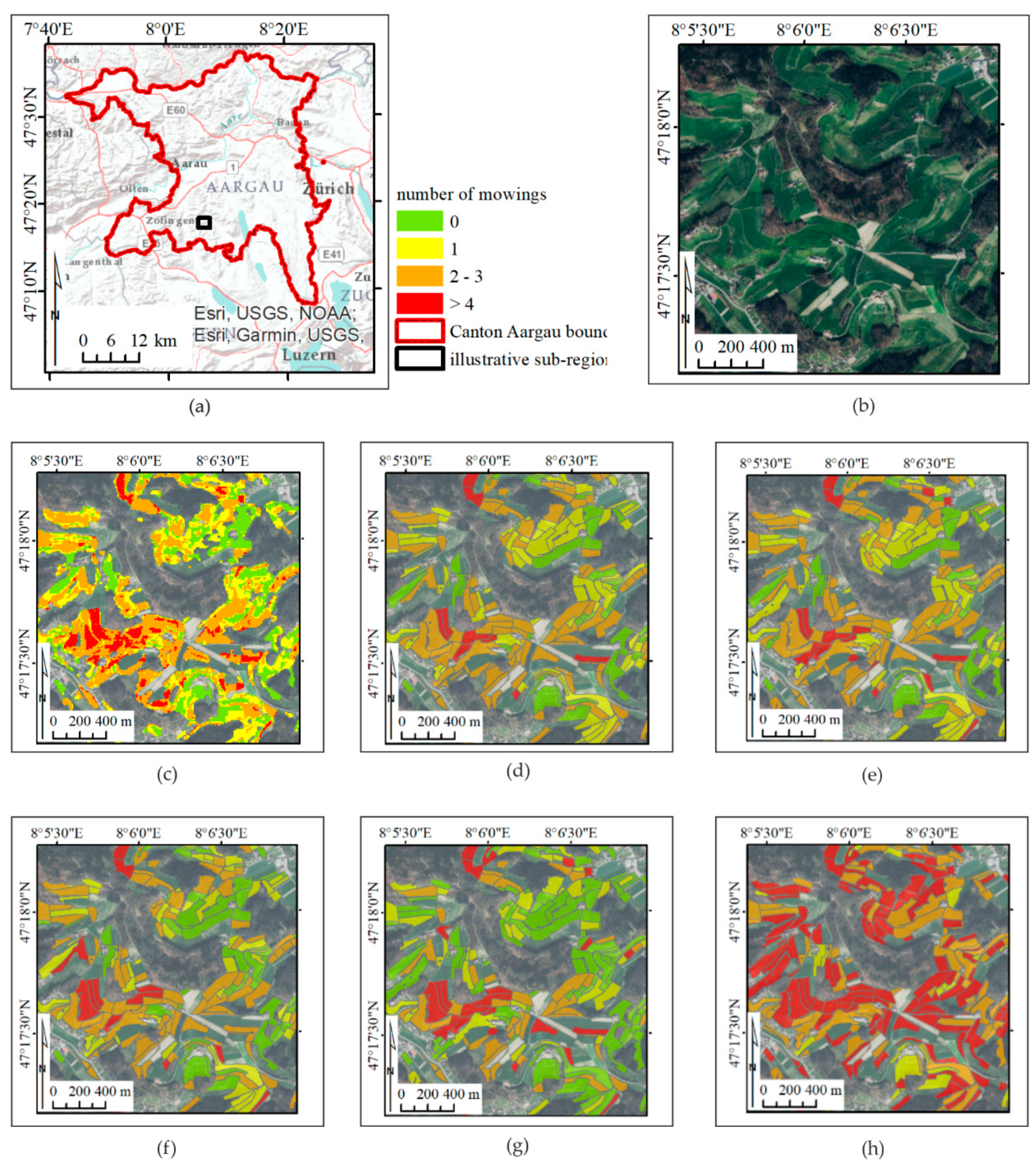
Representative sub-region in the South of Canton Aargau, based on various spatial mapping units, and standard and optimized time series: (a) illustrative sub-region location in Canton Aargau; (b) orthophoto map of the sub-region; (c) Experiment 1a, optimized-pixel; (d) Experiment 1b, optimized-pixel—aggregated to parcels; (e) Experiment 1c, optimized-pixel—aggregated to shrunken parcels; (f) Experiment 2, optimized-parcel; (g) Experiment 3, optimized-shrunken-parcel; and (h) Experiment 4, standard-shrunken-parcel.
Figure 8.
Representative sub-region in the South of Canton Aargau, based on various spatial mapping units, and standard and optimized time series: (a) illustrative sub-region location in Canton Aargau; (b) orthophoto map of the sub-region; (c) Experiment 1a, optimized-pixel; (d) Experiment 1b, optimized-pixel—aggregated to parcels; (e) Experiment 1c, optimized-pixel—aggregated to shrunken parcels; (f) Experiment 2, optimized-parcel; (g) Experiment 3, optimized-shrunken-parcel; and (h) Experiment 4, standard-shrunken-parcel.

Figure 9.
Percentage of grassland parcel area derived from various spatial mapping units and clouds masking levels within GMI categories, and number of detected mowing events: mean and maximum (frequency). Optimized-pixel—aggregated to parcel (OPxP); Optimized-pixel—aggregated to shrunken parcel (OPxSP).

Figure 10.
Percentage of study area in each category of the grasslands mowing index for the reference experiment (optimized-shrunken-parcel) within selected agricultural land use types. The marginal agricultural land use types were not included. artificial meadows (AM); extensively used meadows (EUM); less intensively used meadows (LIUM); permanent meadows (PM); extensively used pastures (EUP); OP, other pastures (pastures at farm borders).

Figure 11.
Average numbers of mowings detected with reduction of input image dataset, grouped by number of initial mowings.
Figure 11.
Average numbers of mowings detected with reduction of input image dataset, grouped by number of initial mowings.


Table 1.
Land use classification accuracy for pixels only within the reference data. optimized-pixel (OPx); standard-pixel (SPx); optimized-parcel (OP); optimized-shrunken-parcel (OSP); standard-shrunken-parcel (SSP).
Table 1.
Land use classification accuracy for pixels only within the reference data. optimized-pixel (OPx); standard-pixel (SPx); optimized-parcel (OP); optimized-shrunken-parcel (OSP); standard-shrunken-parcel (SSP).
| OPx | SPx | OP | OSP | SSP | |
|---|---|---|---|---|---|
| User’s accuracy—grass | 91.2 | 92.1 | 91.7 | 94.6 | 95.3 |
| User’s accuracy-non—grass | 72.7 | 69.3 | 59.7 | 59.5 | 56.3 |
| Producer’s accuracy—grass | 66.8 | 60.3 | 59.0 | 57.3 | 50.7 |
| Producer’s accuracy—non-grass | 93.2 | 94.5 | 91.9 | 95.0 | 96.2 |
| Overall accuracy | 79.7 | 76.9 | 72.1 | 72.3 | 68.8 |
Table 2.
Parcel characteristics of the agricultural land use types. The marginal land use types were not included. OP, other pastures (pastures at farm borders).
Table 2.
Parcel characteristics of the agricultural land use types. The marginal land use types were not included. OP, other pastures (pastures at farm borders).
| Parcel Characteristics—Mean Values | ||||
|---|---|---|---|---|
| Agricultural Land Use Type | Area (ha) | Tree Fraction (%) | Elevation (m) | Slope (deg) |
| AM | 1.20 | 1.6 | 491.9 | 5.6 |
| EUM | 0.47 | 10.5 | 474.2 | 9.0 |
| LIUM | 0.47 | 11.5 | 489.4 | 9.7 |
| PM | 0.85 | 8.5 | 492.5 | 8.6 |
| EUP | 0.73 | 16.5 | 484.5 | 14.0 |
| OP | 1.02 | 10.8 | 488.8 | 9.4 |
Table 3.
Accuracy assessment of analyzed strategies: various spatial mapping units and cloud masking levels, number of correctly detected, and omitted and committed mowing events. r, correlation coefficient; p, significance, Optimized-parcel (OP).
Table 3.
Accuracy assessment of analyzed strategies: various spatial mapping units and cloud masking levels, number of correctly detected, and omitted and committed mowing events. r, correlation coefficient; p, significance, Optimized-parcel (OP).
| Number of Mowing Events | Mean Difference of Number of Mowing Events from OSP | Overall Accuracy (in Relation to OSP) | ||||||
|---|---|---|---|---|---|---|---|---|
| r | p-Value | RMSE | Detected Correctly | Omitted | Committed | |||
| OSP | 0.723 | 0.30 × 10⁻⁸ | 1.058 | 96 | 29 | 9 | - | - |
| OP | 0.705 | 1.11 × 10⁻⁸ | 1.158 | 88 | 37 | 6 | 0.1 | 80.2 |
| OPxP | 0.702 | 1.39 × 10⁻⁸ | 1.039 | 87 | 38 | 4 | 0.3 | 68.7 |
| OPxSP | 0.718 | 0.45 × 10⁻⁸ | 1.149 | 97 | 28 | 8 | 0.1 | 74.7 |
| SSP | 0.416 | 2.64 × 10⁻³ | 2.371 | 116 | 9 | 86 | −2.8 | 4.5 |
© 2018 by the authors. Licensee MDPI, Basel, Switzerland. This article is an open access article distributed under the terms and conditions of the Creative Commons Attribution (CC BY) license (http://creativecommons.org/licenses/by/4.0/).
Share and Cite
MDPI and ACS Style
Kolecka, N.; Ginzler, C.; Pazur, R.; Price, B.; Verburg, P.H. Regional Scale Mapping of Grassland Mowing Frequency with Sentinel-2 Time Series. Remote Sens. 2018, 10, 1221. https://doi.org/10.3390/rs10081221
AMA Style
Kolecka N, Ginzler C, Pazur R, Price B, Verburg PH. Regional Scale Mapping of Grassland Mowing Frequency with Sentinel-2 Time Series. Remote Sensing. 2018; 10(8):1221. https://doi.org/10.3390/rs10081221
Chicago/Turabian StyleKolecka, Natalia, Christian Ginzler, Robert Pazur, Bronwyn Price, and Peter H. Verburg. 2018. "Regional Scale Mapping of Grassland Mowing Frequency with Sentinel-2 Time Series" Remote Sensing 10, no. 8: 1221. https://doi.org/10.3390/rs10081221
Note that from the first issue of 2016, this journal uses article numbers instead of page numbers. See further details here.