Fog and Low Cloud Frequency and Properties from Active-Sensor Satellite Data

Abstract

An analysis of fog and low cloud properties and distribution is performed using satellite-based LiDAR. Recent years have seen great progress in the remote sensing of fog and low clouds using passive satellite-based sensors. On this basis, maps of fog distribution and frequency as well as baseline climatologies have been constructed. However, no information on fog altitude and vertical extent is available in this way, and fog/low cloud below other clouds cannot be detected in most cases. In this study, ten years of observations by the LiDAR aboard the CALIPSO (Cloud-Aerosol LiDAR and Pathfinder Satellite Observations) platform are used to construct a map and statistical evaluations of fog/low cloud distribution and properties. For the purpose of evaluation, a comparison is made to an evaluation of fog/low cloud distribution in Europe, derived from Meteosat measurements using the Satellite-Based Operation Fog Observation Scheme (SOFOS). Both maps show good agreement in spatial patterns in this region with very diverse fog formation mechanisms. It is found that fog/low cloud layers display distinct spatial differences in terms of geometrical thickness and detection accuracy. The number of fog/low cloud instances missed by passive-sensor retrievals due to multi-layer cloud situations is considerable, with clear regional differences.

1. Introduction

Fog and low clouds (FLC) are phenomena that directly and indirectly impact on several human and natural systems: Air and ground-based traffic safety and volume are reduced, with economic impacts, and water is made available to a range of environments. To better understand, characterize and predict FLC situations, accurate knowledge of the spatial and temporal patterns as well as FLC physical properties is required. Satellite data are most suited to provide a coherent data basis given the spatial component of the information required.

In the past, techniques have been developed to use passive-sensor satellite imagery in the visible and infrared ranges to construct such climatologies. Bendix et al. [1] produced a map of FLC frequency in Germany and surrounding regions based on data from the Advanced Very-High Resolution Radiometer (AVHRR). While this and similar maps include a large amount of spatial detail, they are not representative for the entire day, given that AVHRR is mounted on polar-orbiting satellite platforms with infrequent spatial coverage of any given region. This type of problem was overcome when improved spectral capabilities allowed for FLC detection on the basis of geostationary satellite data with the advent of the Spinning-Enhanced Visible and Infrared Imager (SEVIRI) aboard the Meteosat Second Generation (MSG) satellites. Climatological distributions of FLC for Europe have been produced on the basis of the Satellite-based Operational Fog Observation Scheme (SOFOS, [2]) by Cermak et al. [3], and updated by Egli et al. [4]. However, the detection of FLC in these studies is incomplete, with hit rates for SOFOS at 63 to 70% [2] and 43% [4]. The non-detection of a third to more than half of FLC situations has been explained by small-scale features too thin or small for the satellite footprint (3–5 km resolution in Europe), general classification errors, and multi-layer cloud situations, where another cloud is above a FLC situation, rendering the latter invisible in the passive-sensor satellite data [2]. So far, it has not been possible to quantify the relative contributions of each of these error sources.

Active-sensor satellite data, in particular the space-based LiDAR aboard the Cloud-Aerosol LiDAR and Infrared Pathfinder Satellite Observations (CALIPSO) system, has proven very capable at detecting the presence and altitude of atmospheric features such as clouds (e.g., [5]). With respect to FLC observations, CALIPSO has thus proven very useful as an independent source of validation data in regions where other evaluation data sets are largely absent [6].

However, since CALIPSO is a nadir-pointing polar-orbiting system, repeated observations of the same location are far between. Nonetheless, global climatologies of a range of features have been constructed in the past using spatial averaging (e.g., [7]). So far, no climatological evaluation of FLC presence and properties has been performed based on CALIPSO data despite the obvious potential for expanding present-day knowledge of FLC.

On this basis, the following research questions are identified for the present study:

(1)

Can CALIPSO data be used to plausibly represent FLC distribution?

(2)

Are there distinct differences in FLC properties between FLC regimes?

(3)

How frequent are FLC situations below other clouds?

2. Data and Methods

Europe was chosen as the analysis region for this study. There are two reasons for this: On the one hand, passive-sensor FLC baseline climatologies are available for qualitative comparison in this region [4,8]. On top of this, Europe features a relatively complex combination of continental and marine fog regimes in a comparatively small area and thus seems well-suited for an objective analysis.

For the study of FLC presence, the CALIPSO level 2 1 km cloud-layer product was chosen (version 3.30, and 3.01 where the former was not available). While this space-based LiDAR product can reliably detect cloud layers even under thin aerosol or cloud layers higher up in the atmosphere, multi-layer detection will only work as long as these overlying layers are not optically opaque.

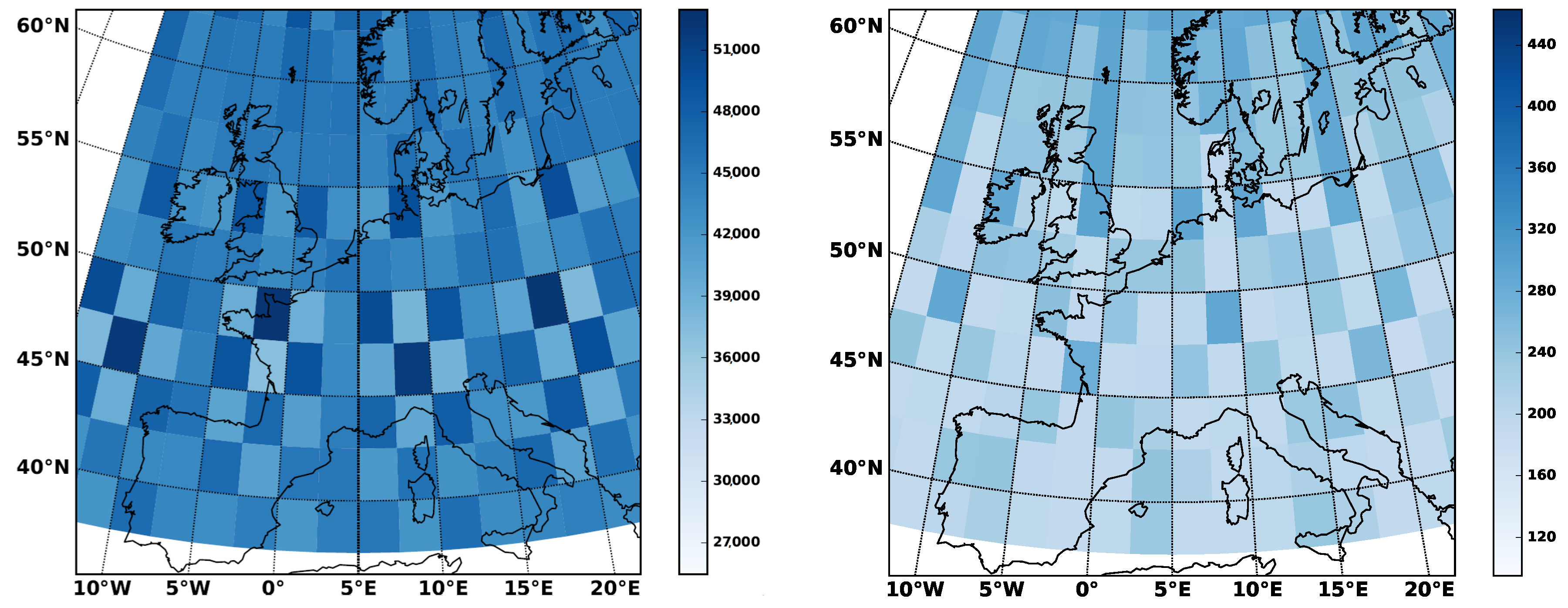
To increase the sample size for this study, both daytime and night-time CALIPSO overpasses were included in the analysis. Since winter is the season with the most pronounced FLC occurrence in Europe (e.g., [4]), data was used for December, January and February (DJF) of the ten available winters, 2006/2007 to 2015/2016. In total, 5641 overpasses were available for the region. To further increase the sample size, data were aggregated in grid cells of 2.5${}^{°}$ latitude by 2.5${}^{°}$ longitude. In each of these cells, between 20,000 and 50,000 data points were available in a few hundred overpasses per grid cell, as shown in Figure 1.

To derive a count of overpasses with FLC for each grid cell, the following procedure was applied:

• Feature altitude above the terrain was computed for each LiDAR profile by subtracting the terrain elevation included in the CALIPSO cloud-layer product from the reported feature altitude. This was done to eliminate terrain effects, in particular over mountaineous regions.
• For each individual LiDAR profile available within a given grid cell, it was tested whether in the lowermost cloud layer cloud top was at or below 2000 m; this threshold was chosen as a cut-off level for low clouds, and is consistent with Cermak et al. [3]. Also, cloud base had to be at or below 500 m to ensure proximity to the surface. This comparatively high altitude was chosen as the cloud-base criterion so as not to exclude too many situations with optically opaque clouds, in which the LiDAR signal will be fully attenuated. A LiDAR profile was classified as an ‘FLC profile’ where both cloud altitude criteria were met.
• A given overpass over a given grid cell was classified as an ‘FLC overpass’ if at least 10% of the LiDAR profiles of the overpass within the cell were identified as FLC profiles. There is no specific physical basis for this precise threshold, but it appeared very plausible in careful screening of many overpasses.
• To characterize the FLC overpasses, additional information was extracted from the CALIPSO cloud-layer product for these situations: FLC geometrical thickness, the presence of other cloud layers above the FLC, and the cloud-aerosol discrimination (CAD) score for the FLC feature, which reports the certainty with which a given feature is classified as a cloud [5].

Since the individual grid cells still appear to show artifacts of the overpasses (cf. 45${}^{°}$N to 50${}^{°}$N in Figure 1), sample size was further increased by aggregation. Two methods were pursued: Aggregation by latitude as an objective approach, and aggregation by four regions seen as representative of specific fog regimes present in Europe. These regions are shown in Figure 2, and encompass the following:

• Atlantic—oceanic conditions
• Baltic—cold-marine conditions
• Mediterranean—warm-marine conditions
• Continental—continental conditions

3. Results and Discussion

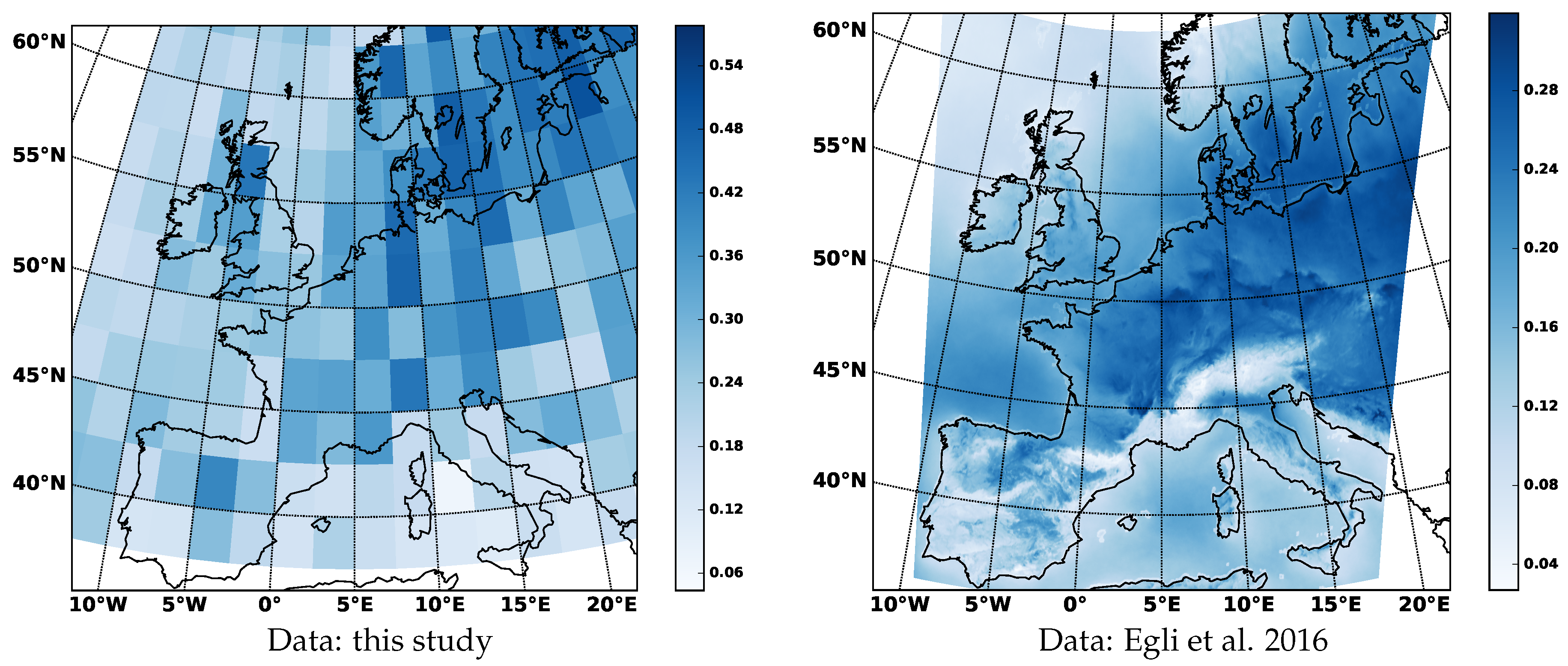
Figure 3 highlights the general patterns found in the distribution of FLC frequency found for DJF in this study and in Egli et al. [4] based on the SOFOS method [2,9]. Given the vastly different approaches used in the generation of both data sets, this is intended as no more than a qualitative plausibility check. In particular, the data sets juxtaposed in this figure differ in the following central aspects:

• The CALIPSO data set builds on up to two observations per 24-hour period, the Meteosat data on continuous geostationary observations.
• In contrast to the CALIPSO data set, the Meteosat data set does not contain information on FLC below other clouds.
• While the Meteosat data set considers the situation in individual pixels, the CALIPSO data set presents an aggregation in larger grid cells that do not have to be entirely covered by FLC to be counted (see Section 2).

Against this background, a quantitative comparison would not be reasonable. However, despite the differences in the data sets, an agreement is found in the general regional patterns of FLC distribution. In particular, the Baltic sea region is marked by the highest frequencies in both data sets, and there is a general tendency towards lower FLC frequencies from North to South. In some regions, FLC patches are well represented in the CALIPSO data set, e.g., in Northern Spain; in other places local detail is lost however, e.g., in the Po valley of Northern Italy.

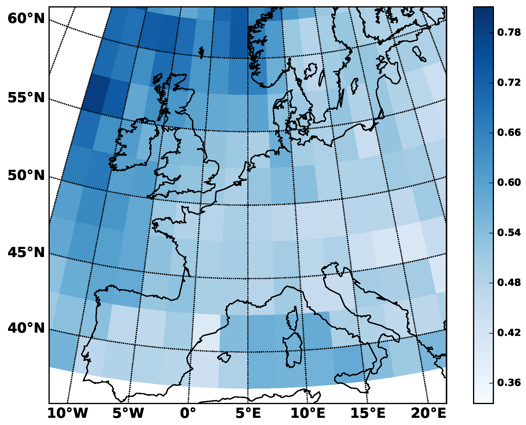
In addition to the distribution of FLC situations, the profile information obtained by space-based LiDAR allows for a characterization of the average vertical extent of FLC situations, as shown in Figure 4. A clear pattern with greater average thickness over the Atlantic ocean and the Mediterranean sea as compared to the land masses is seen here. This may possibly be due to greater cloud water availability over the water masses and warm advection.

Despite the apparent plausibility of the map presentations of FLC distribution, regionally aggregated analysis appears more robust given the relatively small sample sizes. The following analysis builds on the sectoring shown in Figure 2, and on latitudinal aggregation.

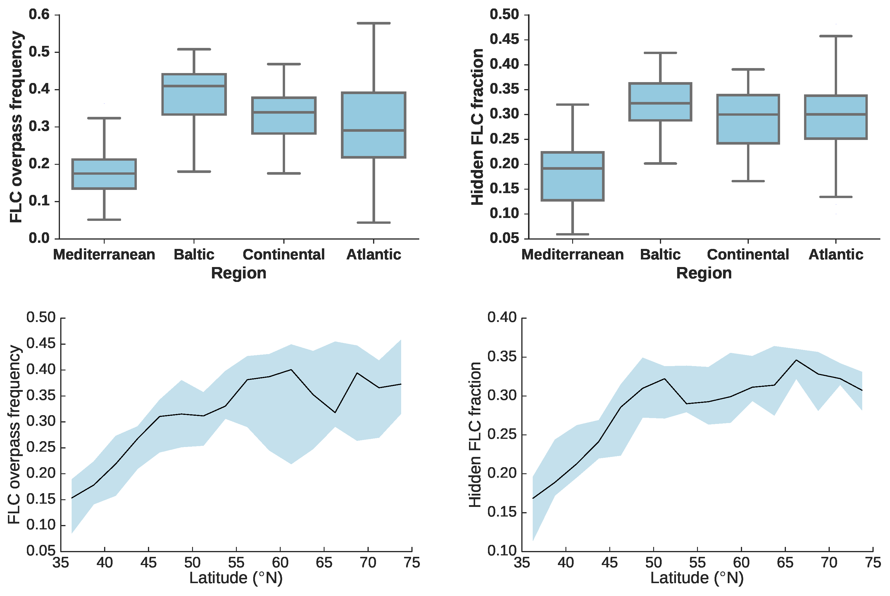
Figure 5 shows evaluations of several parameters on a regional/latitudinal level. As expected and already seen in the map (Figure 3) the frequency of FLC overpasses is greatest in the Baltic region with a median at about 40% and lowest in the Mediterranean with a median at roughly 18%. The continental and Atlantic regions are in between these (median around 30 to 35%), with a higher variability in the Atlantic region. Similarly, the latitudinal aggregation (bottom row of Figure 5) reveals an increase in FLC overpass frequency from South to North, with a stabilization around 50${}^{°}$N. Variability, as indicated by the inter-quartile range, is remarkably large north of 50${}^{°}$N; this is explained by the pronounced difference between the regions, as seen in the left-hand panel of Figure 3.

The FLC situations underneath another cloud as a fraction of all FLC situations (‘hidden FLC fraction’) is similar in the Baltic, continental and Atlantic regions, and more generally north of about 47${}^{°}$N, with a median value of around 30% in each region. In the Mediterranean region, the median is lower, at just below 20%. This very likely provides an explanation for the reduced hit rates in passive-sensor FLC detection techniques: FLC underneath another cloud will not be detected. Given that Cermak and Bendix [2] detected 63–70% of FLC situations from passive-sensor data and 25–30% of such situations are masked by higher-level clouds, errors due to other sources likely are less important than multi-layer situations. In the case of the Egli et al. [4] implementation of the passive-sensor technique with a hit rate of 43%, errors due to other difficulties likely appear more frequently, as discussed in that paper.

Finally, the Cloud-Aerosol-Discrimination (CAD) score reported in the CALIPSO product set is an indication of the certainty with which a feature was identified as cloud or aerosol. A value of 100 indicates a certain detection of cloud, −100 indicates aerosol [10,11]. In the Baltic, continental and Atlantic regions, CAD is at 100 almost always (not shown)—the FLC situations identified are very likely to actually be clouds in almost all cases. In the Mediterranean region or the southernmost latitudes however, a slightly wider distribution is found. This may be an indication of hazy situations making up a portion of the FLC identified in the Mediterranean region.

4. Conclusions and Outlook

The method applied in this study has several shortcomings when used in the analysis of average FLC conditions: It relies on up to two time steps over a day, it is made up of sparse overpasses of a sensor with only a very small footprint, and the averaging performed rests on the assumption that there were no significant trends over the 10-year period considered. Nonetheless, for the reasons presented in the manuscript, insights can be gained from careful consideration of the aggregated data set (research question 1 above).

In this way, the evaluation of ten years of observations by space-based LiDAR on CALIPSO has led to new insights about the distribution of FLC. Spatial patterns obtained for Europe are similar to those seen in ten years of Meteosat observations, despite the sparsity of observations available from CALIPSO. Distinct differences between regions within Europe can be discerned in terms of FLC frequency and CAD score (research question 2). Analysis of multi-layer cloud situations reveals that in most regions, about a quarter of FLC situations are underneath other clouds, thus making detection impossible for present-day generation passive-sensor FLC detection techniques, and accounting for much of the error in these (research question 3). Given that CALIPSO cloud layer detection will be impeded in cases of opaque overlying clouds, the actual number of ‘hidden’ FLC situations may actually be even greater than shown in this study.

The main benefit of active-sensor evaluations as presented here over a passive-sensor evaluation is the potential to explicitly derive information on the vertical distribution of FLC, including in situations with several feature layers. A future challenge will be to find a way to combine the specific advantages of passive and active satellite-based sensor systems to fully characterize FLC situations.

References

- Bendix, J.; Thies, B.; Nauss, T.; Cermak, J. A feasibility study of daytime fog and low stratus detection with TERRA/AQUA-MODIS over land. Meteorol. Appl. 2006, 13, 111–125. [Google Scholar] [CrossRef]
- Cermak, J.; Bendix, J. A Novel Approach to Fog/Low Stratus Detection using Meteosat 8 Data. Atmos. Res. 2008, 87, 279–292. [Google Scholar] [CrossRef]
- Cermak, J.; Eastman, R.M.; Bendix, J.; Warren, S.G. European climatology of fog and low stratus based on geostationary satellite observations. Q. J. R. Meteorol. Soc. 2009, 135, 2125–2130. [Google Scholar] [CrossRef] [Green Version]
- Egli, S.; Thies, B.; Drönner, J.; Cermak, J.; Bendix, J. A 10 year fog and low stratus climatology for Europe based on Meteosat Second Generation data. Q. J. R. Meteorol. Soc. 2017, 143, 530–541. [Google Scholar] [CrossRef]
- Vaughan, M.A.; Powell, K.A.; Winker, D.M.; Hostetler, C.A.; Kuehn, R.E.; Hunt, W.H.; Getzewich, B.J.; Young, S.A.; Liu, Z.; McGill, M.J. Fully Automated Detection of Cloud and Aerosol Layers in the CALIPSO Lidar Measurements. J. Atmos. Ocean. Technol. 2009, 26, 2034–2050. [Google Scholar] [CrossRef]
- Cermak, J. Low clouds and fog along the South-Western African coast—Satellite-based retrieval and spatial patterns. Atmos. Res. 2012, 116, 15–21. [Google Scholar] [CrossRef]
- Stephens, G.; Winker, D.; Pelon, J.; Trepte, C.; Vane, D.; Yuhas, C.; L’Ecuyer, T.; Lebsock, M. CloudSat and CALIPSO within the A-Train: Ten Years of Actively Observing the Earth System. Bull. Am. Meteorol. Soc. 2018. [Google Scholar] [CrossRef]
- Cermak, J.; Bendix, J. Detecting Ground Fog From Space—A Microphysics-Based Approach. Int. J. Remote Sens. 2011, 32, 3345–3371. [Google Scholar] [CrossRef]
- Cermak, J.; Bendix, J. Dynamical Nighttime Fog/Low Stratus Detection Based on Meteosat SEVIRI Data: A Feasibility Study. Pure Appl. Geophys. 2007, 164, 1179–1192. [Google Scholar] [CrossRef]
- Fuchs, J.; Cermak, J. Where Aerosols Become Clouds—Potential for Global Analysis Based on CALIPSO Data. Remote Sens. 2015, 7, 4178–4190. [Google Scholar] [CrossRef] [Green Version]
- Yang, W.; Marshak, A.; Várnai, T.; Liu, Z. Effect of CALIPSO cloud-aerosol discrimination (CAD) confidence levels on observations of aerosol properties near clouds. Atmos. Res. 2012, 116, 134–141. [Google Scholar] [CrossRef]
Figure 1.
Number of individual data points (left), and overpasses (right) available in each grid cell over the period considered.
Figure 2.
Regions over which FLC data were aggregated.
Figure 3.
Relative frequency of days with DJF FLC in each grid box based on CALIPSO observations (left, this study), and relative frequency of hours with DJF FLC in each pixel based on SEVIRI observations, 2005 to 2016 (right, [4]). Since CALIPSO is only available up to twice a day whereas up to 96 scenes are considered in the SEVIRI evaluation, the two panels can only be compared qualitatively.
Figure 4.
Average geometrical thickness of FLC layers detected (km).
Figure 5.
Frequency of overpasses with FLC, and fraction of these FLC situations hidden below another cloud layer. Values for all the grid boxes contained within each region are given at the top, where boxes contain the second and third quartiles separated by the median line, and whiskers extend up to the highest and lowest values within 1.5 standard deviations. At the bottom, the same is shown averaged over latitude instead of regions, with the median shown in black and the second and third quartiles shaded.
© 2018 by the author. Licensee MDPI, Basel, Switzerland. This article is an open access article distributed under the terms and conditions of the Creative Commons Attribution (CC BY) license (http://creativecommons.org/licenses/by/4.0/).
Share and Cite
MDPI and ACS Style
Cermak, J. Fog and Low Cloud Frequency and Properties from Active-Sensor Satellite Data. Remote Sens. 2018, 10, 1209. https://doi.org/10.3390/rs10081209
AMA Style
Cermak J. Fog and Low Cloud Frequency and Properties from Active-Sensor Satellite Data. Remote Sensing. 2018; 10(8):1209. https://doi.org/10.3390/rs10081209
Chicago/Turabian StyleCermak, Jan. 2018. "Fog and Low Cloud Frequency and Properties from Active-Sensor Satellite Data" Remote Sensing 10, no. 8: 1209. https://doi.org/10.3390/rs10081209
Note that from the first issue of 2016, this journal uses article numbers instead of page numbers. See further details here.