Unsupervised Segmentation Evaluation Using Area-Weighted Variance and Jeffries-Matusita Distance for Remote Sensing Images

1
State Key Laboratory of Resources and Environmental Information System, Institute of Geographical Sciences and Natural Resources Research, Chinese Academy of Sciences, Beijing 100101, China
2
University of Chinese Academy of Sciences, Beijing 100049, China
*
Author to whom correspondence should be addressed.
Remote Sens. 2018, 10(8), 1193; https://doi.org/10.3390/rs10081193
Submission received: 26 June 2018
/
Revised: 20 July 2018
/
Accepted: 20 July 2018
/
Published: 30 July 2018
(This article belongs to the Special Issue Pattern Analysis and Recognition in Remote Sensing)
Abstract
:Image segmentation is an important process and a prerequisite for object-based image analysis. Thus, evaluating the performance of segmentation algorithms is essential to identify effective segmentation methods and to optimize the scale. In this paper, we propose an unsupervised evaluation (UE) method using the area-weighted variance (WV) and Jeffries-Matusita (JM) distance to compare two image partitions to evaluate segmentation quality. The two measures were calculated based on the local measure criteria, and the JM distance was improved by considering the contribution of the common border between adjacent segments and the area of each segment in the JM distance formula, which makes the heterogeneity measure more effective and objective. Then the two measures were presented as a curve when changing the scale from 8 to 20, which can reflect the segmentation quality in both over- and under-segmentation. Furthermore, the WV and JM distance measures were combined by using three different strategies. The effectiveness of the combined indicators was illustrated through supervised evaluation (SE) methods to clearly reveal the segmentation quality and capture the trade-off between the two measures. In these experiments, the multiresolution segmentation (MRS) method was adopted for evaluation. The proposed UE method was compared with two existing UE methods to further confirm their capabilities. The visual and quantitative SE results demonstrated that the proposed UE method can improve the segmentation quality.
1. Introduction
With the rapid development of high-resolution satellite sensor technology, the phenomenon often occurs that different geo-objects have the same spectral reflectance, or the same geo-objects have different spectral reflectance in a high spatial resolution (HSR) remote sensing image, thus, resulting in the poor performance of traditional pixel-based image analysis in HSR images. Geographic object-based image analysis (GEOBIA) has become increasingly important as a new and evolving paradigm in remote-sensing translation and analysis [1,2] because of its lower sensitivity to the spectral variance within geo-objects [3]. In addition, the spectral, textural, and contextual information, and geo-object features could be effectively used by GEOBIA to improve the subsequent classification accuracy [4,5,6]. GEOBIA for a remote sensing image includes three main steps, i.e., image segmentation, information extraction, and segments classification [7,8].
The image segmentation process, which partitions a remote sensing image into spatially contiguous and spectrally homogeneous regions [9], is commonly considered to be a prerequisite for GEOBIA because GEOBIA performance is directly affected by the segmentation quality. Following the studies on this task, many segmentation methods have been proposed, such as the deep learning method [10], fractal network evolutionary approach (FNEA) [11], multi-resolution recursive spanning tree method [12], watershed segmentation [13,14], spectral segmentation [15], and multi-resolution segmentation (MRS) [16]. In the aforementioned segmentation methods, the “scale” parameter is used to control the sizes of the segments, and different scales can lead to different segmentation results. Hence, the evaluation of segmentation quality is considered to be important for GEOBIA in determining optimal scales and obtaining effective segmentation results for subsequent analysis.
Since segmentation quality has been shown to have an impact on GEOBIA, some scholars have focused on image segmentation evaluation methods to determine good segmentation scales [4,8,17,18,19,20,21]. In general, the segmentation evaluation methods can be grouped into three strategies: Visual analysis, supervised evaluation (SE), and unsupervised evaluation (UE) [4,22,23,24]. Visual analysis methods involve users determining the optimal scales that can produce good segmentations by visually comparing multiple segmentations, and it has been applied in several studies [25,26,27]. However, the greatest problem of the method is that it is highly subjective and time-consuming because a set of segmentations needs to be inspected in detail to determine the best one, and opinions vary on the best segmentation. SE methods evaluate segmentations by comparing the segmentation results with reference images, and this comparison involves computing some dissimilarity measures to determine the segmentation that best matches the reference [8,18,19,28,29,30,31]. It is the most commonly used segmentation evaluation strategy because the methods can allow for the determination of the most accurate segmentation relative to the objects that the user believes are important [19]. However, the limitations of SE methods are that the reference image is generated by human interpretation and the creation of reference polygons can be subjective and time-consuming. Compared with visual and SE methods, UE methods are completely independent of expert knowledge without needing a reference polygon [32], and the segmentation quality is evaluated according to certain measures, which are typically established in agreement with human perception of what makes a good segmentation [24]. This makes it more efficient and less subjective than the other two methods. Thus, much effort has been put into the UE methods recently [17,20,21,22,33,34,35].
UE methods consider that a good segmentation should have two desirable properties: Each segment should be internally homogeneous and should be distinguishable from its neighbors [36]. Hence, most UE methods involve calculating intrasegment homogeneity and intersegment heterogeneity measures and then aggregating these values into a global value [21,23,24,29,32,36,37,38,39]. For example, the area-weighed variance (WV) and global Moran’s I (MI) were used to calculate the intrasegment homogeneity and intersegment heterogeneity, respectively, in Espindola et al. [36], Johnson and Xie [24], and Johnson et al. [21] articles. Zhang et al. [23] proposed an unsupervised remote sensing image evaluation method using the T method to calculate the homogeneity and the D method to calculate the heterogeneity. Although these existing methods could be helpful to the automation of selecting the optimal scale parameters, they ignored the fact that the homogeneity measures are a local evaluation criteria, whereas the heterogeneity measures are a global evaluation criteria. Due to the difference in the homogeneity and heterogeneity evaluation criteria characteristics, this may cause a biased segmentation result, i.e., an over- or under-segmented result. In addition, the combination strategies for the homogeneity and heterogeneity measures must be carefully designed to achieve the potential trade-offs of different measures. When the number of measures is large, combining them is difficult.
This paper addressed these issues by proposing a new unsupervised remote sensing image segmentation evaluation method using the area-weighted variance (WV) and Jeffries-Matusita (JM) distance. The WV and JM distance were used to calculate the homogeneity and heterogeneity, respectively. Both of these metrics are local measure criteria, which may solve the problem of a biased segmentation result caused by the difference in the homogeneity and heterogeneity of the evaluation criteria characteristics. At the moment, the contribution of the common border between adjacent segments and the area of each segment are integrated into the JM distance formula, which could make the heterogeneity measure more effective and objective. Then, the WV and JM distance were combined to reveal the segmentation quality by capturing the trade-offs of the two measures. In this paper, to achieve potential trade-offs of different measures, the effectiveness of the three combination strategies by means of a geometric illustration is revealed. The remainder of the paper is organized as follows. In Section 2, the details of the proposed method are described, with a particular focus on the JM distance that considers the contribution of the common border between adjacent segments and the area of each segment. Then, a description of the study areas and images, as well as the result analyses, follows in Section 3. In Section 4 and Section 5, the discussion and conclusions are presented, respectively.
2. Materials and Methods
2.1. Overview
A schematic of calculating the WV and JM distance measures to evaluate the segmentation quality is shown in Figure 1. First, we calculated the WV values to represent the homogeneity of the segmentation result. Second, the JM distance was improved by considering the contribution of the common border between adjacent segments and the area of each segment was calculated to represent the heterogeneity. Third, the two measures were jointly used to assess the segmentation quality. Furthermore, the two measures can be combined into a single measure to evaluate the segmentation quality.
2.2. Area-Weighted Variance (WV) and Jeffries-Matusita (JM) Distance Measures
Most UE methods in remote sensing usually consider that the segmentation result at the optimal scale should, on average, be internally homogeneous and externally heterogeneous. These criteria fit with what is generally accepted as a good segmentation for natural images [25]. The existing methods consist of two components: A measure of within-segment homogeneity and one of between-segment heterogeneity. Then, the results are aggregated. First, the WV was used to measure the global intra-segment goodness and was weighed by each segment’s area. It is defined as follows:
where is the area, is the variance averaged across all bands of segment i, n is the number of segments, m is the number of bands of remote sensing image, and is the variance of segment i in band b. The variance was chosen as the intra-segment homogeneity measure because relatively homogeneous segments generally have low variance. The variance was averaged across all bands to take full use of the band information occupied by the remote sensing image. The area-weighted variance was used for the global calculation so that large segments have more influence on global calculations than small ones. Second, the region adjacency graph (RAG) was built to simplify the evaluation processing. The RAG is an undirected graph, which is used to express the spatial relationship between adjacent segments, with nodes representing segments and arcs representing their adjacency [40,41]. Third, the JM distance of each pair of segments was calculated based on the RAG as follows:
where is the Bhattacharyya distance, and are the means, and and are the variance of adjacent segments i and j, respectively. The JM distance is a widely used measure of the spectral separability distance between the two class density functions [42,43]. If two adjacent segments are regard as two classes, it is reasonable to use the JM distance to measure the spectral heterogeneity. As shown in Figure 2, in the case that Segment1’ and Segment2 are regarded as two geo-objects, Segment1 is considered to be over-segmented and Segment1” is considered to be under-segmented. The JM values between adjacent segments from Figure 2a–c are 1.96, 1.75, and 1.35, respectively. From over-segmentation to under-segmentation, the JM value is decreasing. Thus, the relatively heterogeneous segments generally have low JM distances. Fourth, the relative JM distance can be calculated as the heterogeneity of each segment, which weights the contribution of the common border of a segment and its neighboring segments as follows:
where is the boundary length of segment i, and , and are the common border and the JM distance of segment i and its neighboring segment k, respectively. The common border-weighed JM distance is used for each segment calculation so that the neighboring segments, which have a large common border, have more of an impact than small ones. Fifth, the average JM distance can be calculated by being averaged across all bands as follows:
where is the JM distance of segment i in band b. Finally, the inter-segment global goodness can be measured across all segments, which weights the contribution of each segment by its area as follows:
The WV and JM distance measures were jointly used to assess the segmentation quality. Lower WV values and JM values indicate segmentation levels with higher within-segment homogeneity and inter-segment heterogeneity, respectively. In an ideal case, both the WV and JM distance measures achieve the lowest values of 0 for a good segmentation. Moreover, the joint use of the two measures can indicate both over- and under-segmentation and is not biased toward over- or under-segmented images. When an image is over-segmented, the WV value is small, but the JM value increases to incur the penalty. By contrast, when an image is under-segmented, the JM value is small, but the WV value increases.
2.3. Combination of WV and JM Distance Measures
As previously mentioned, if the WV and JM values of one segmentation are both lower or both higher than those of another segmentation, it will be easy to distinguish the better segmentation. However, when the two measure values of one segmentation are not concurrently higher or lower than those of another segmentation, it will be difficult to determine the better segmentation. To deal with this complexity, the WV and JM distance measures can be combined into a single measure to capture the trade-off between the two measures. However, the effectiveness of the combined measures can be directly affected by the way in which they are combined. Accordingly, this paper compared three combination strategies to reveal the effectiveness.
The first combination strategy is the F-measure [21], which is defined as follows:
where the weight α is a constant 0.5 in this paper. The value of the F-measure varies from 0 to 1, with higher values indicating higher segmentation quality. The WV and JM values are both normalized to a 0–1 range, in which higher values indicate higher homogeneity and higher values indicate higher heterogeneity. They are defined by:
The second combination strategy is the Z method [23], with lower values indicating higher segmentation quality, which is defined as:
The third strategy is the LP method, which is considered as the signal for the optimal scale parameterization [29]. The LP is defined as:
where H(l) is the H value at scale parameter l, and denotes the interval of the scale parameter. Specifically, the largest value of represents the optimal scale parameter and good segmentation.
2.4. Comparison with Existing UE Methods
To demonstrate the effectiveness of the proposed UE method, this paper first selected the best combination strategy by comparing the above-mentioned combination strategies. Then, the two methods by Zhang et al. [23] and Espindola et al. [36] were compared to the proposed method. All measures are sensitive to both over-segmentation and under-segmentation when two partitions are compared. The reason for selecting these two UE methods for comparison is that they both follow the characteristic criteria, similar to the proposed method. In addition, in the existing two methods, the heterogeneity measures are both global criteria, because Moran’s I and D measures are calculated based on the mean gray value of the entire image, which are different from the JM distance.
2.5. SE Methods
The SE methods of the quality rate (QR), under-segmentation (US), over-segmentation (OS) and an index of combining the US and OS (D) were used to validate the effectiveness of the proposed UE method. The QR index ranges from 0 to 1 and measures the discrepancy in the area between a reference polygon and its corresponding segment. Note that lower values of QR indicate less discrepancy in the area, and, thus, a more accurate segmentation. The US, OS and D can reflect the geometric relationships between the reference polygons and the corresponding segments. In particular, zero values for US and OS indicate that there are no over-segmented and under-segmented objects, respectively. Since both US and OS are normalized indices between 0 and 1, the composite index D is reasonable enough to equally value these two indices. Thus, a lower value of D reflects a higher overall segmentation quality considering both the over-segmentation and under-segmentation. The details on these metrics can be found in Clinton et al. [19].
2.6. Image Segmentation Method
Of the various image segmentation methods, the region-based method is particularly suitable and, thus, widely used for remote sensing image segmentation [44,45,46]. The region-based method can produce spatially contiguous regions that have inherent continuous boundaries. At the moment, these regions can be regarded as geo-objects directly. In this paper, the multiresolution segmentation (MRS) method [47] embedded in the commercial software eCognition Developer 8.7 was chosen and evaluated to show the effectiveness of the proposed UE method.
The MRS method uses a bottom-up region growing strategy starting from the pixel level based on the local-mutual best merging. The scale parameter is the stop criterion for the optimization process. If the resulting increase in heterogeneity when fusing two adjacent objects exceeds a threshold determined by the scale parameter, then no further fusion takes place, and the segmentation stops. The shape and compactness parameters range from 0 to 1. If the shape parameter is set as small, the MRS will concentrate on generating segments with spectral homogeneity. By contrast, if the shape parameter is set as large, the segments will likely have a regular shape and neglect the spectral constraint. In this paper, the segmentation was implemented at the scale parameter with a range from 8 to 20, whereas the other two parameters were fixed to their default values (shape: 0.1, compactness: 0.5). The range of the scale parameter was selected by taking into account the sizes of geo-objects in the experimental image.
3. Results
3.1. Study Area and Image
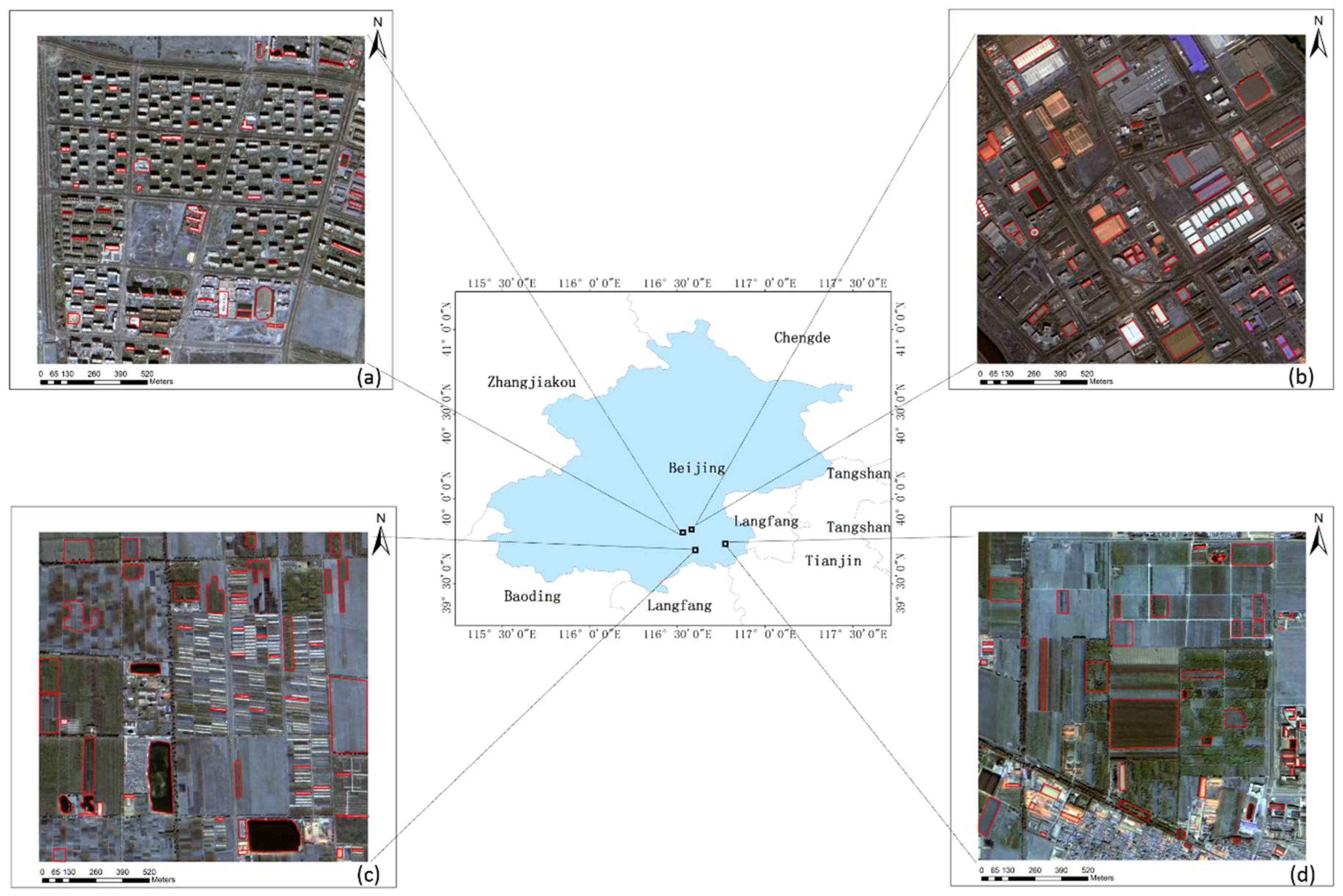
A gaofen-1 (GF-1) scene in Beijing, China, which was acquired on 8 May 2016, was used as the image data. The GF-1 images, which were obtained by the panchromatic and multispectral (PMS) sensor, contain four multi-spectral bands (blue, green, red, and near infrared) and a panchromatic band. The multispectral and panchromatic images were fused to produce a four-band pan-sharpened multispectral image with 2 m resolution using the NNDiffuse Pan Sharpening function from ENVI 5.2 software. Four test image areas of an industrial area, a residential area, and two farmland areas in the GF-1 scene were used to show the segmentation evaluation results (Figure 3). The one farmland area includes vegetation, farmland, water, and a cultivation hothouse (Figure 3c), and the other includes a forest, farmland, and a village (Figure 3d). The image sizes are all 1.6 × 1.6 km.
3.2. Effectiveness Analysis of the WV and JM Distance Measures
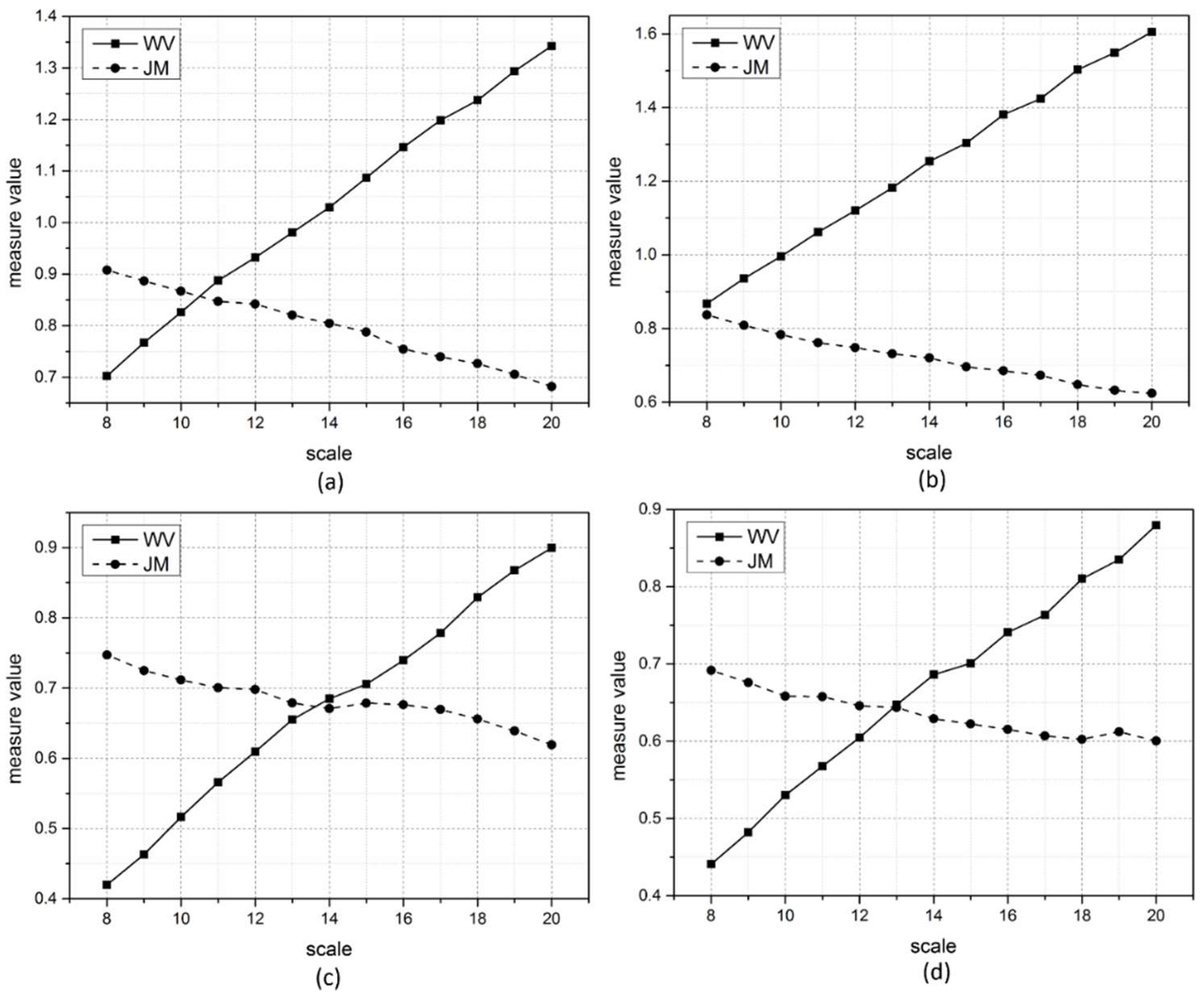
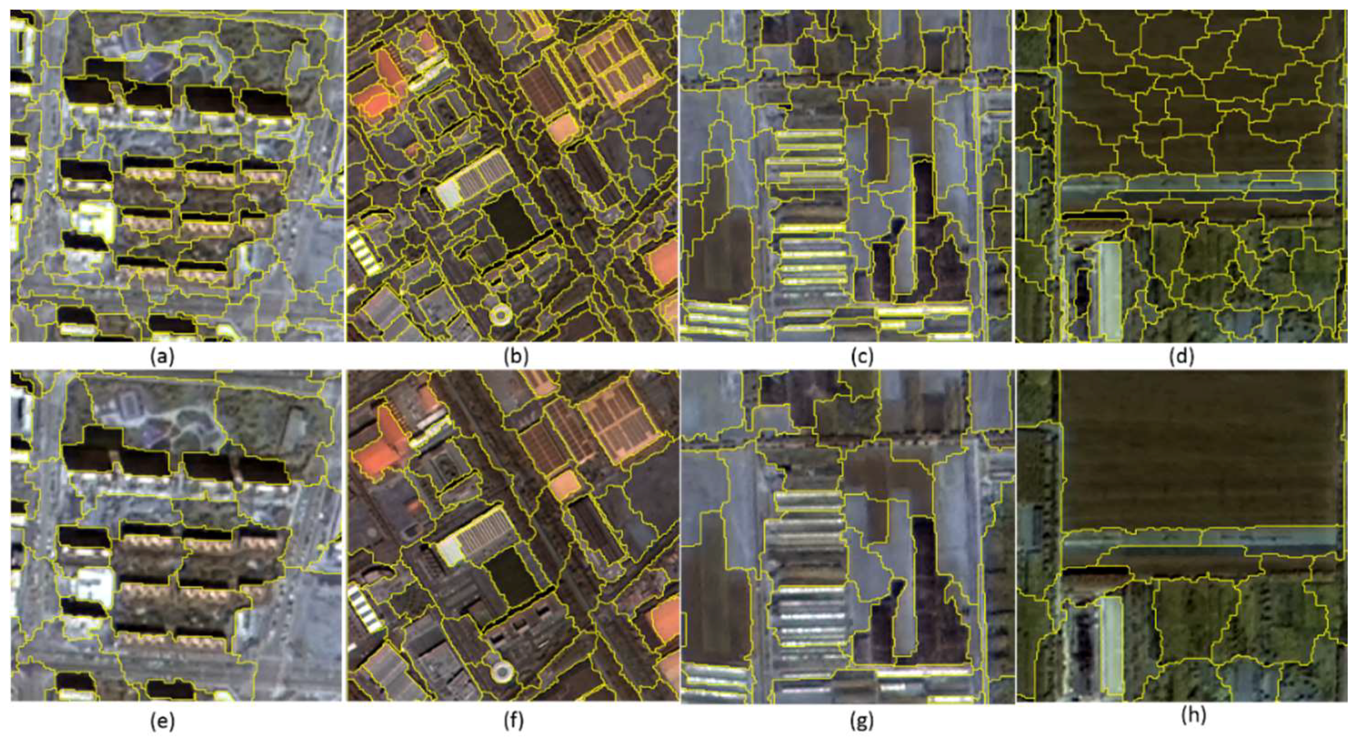
The MRS method was applied in the four study areas to produce 13 segmentation results for each study area with the scale of 8–20, respectively. Then, the WV and JM distance measures were calculated for each segmentation result to demonstrate the effectiveness of the two measures, as shown in Figure 4. From the visual assessment, the segmentation at scale 8 is apparently over-segmented, while the one at scale 20 is apparently under-segmented (Figure 5). When over-segmented, the homogeneity indicator WV is small, while the heterogeneity indicator JM is large because the segmentations have a high within-segment homogeneity and low inter-segment heterogeneity in this case. However, when they are under-segmented, the WV value is large, and the JM value is small because the homogeneity within segments decreases and the heterogeneity between segments increases. From scale 8 to 20, the WV value is increasing, and the JM value is decreasing gradually for the four study areas of the T1, T2, T3, and T4 images. The WV and JM distance measures can reflect the change in image quality during a coarsening of the segmentation scales, but it cannot directly reveal the optimal scale parameters. The combination of the WV and JM distance measures resolves these difficulties, as discussed in the next subsection.
3.3. Effectiveness Analysis of Different Combined Measures
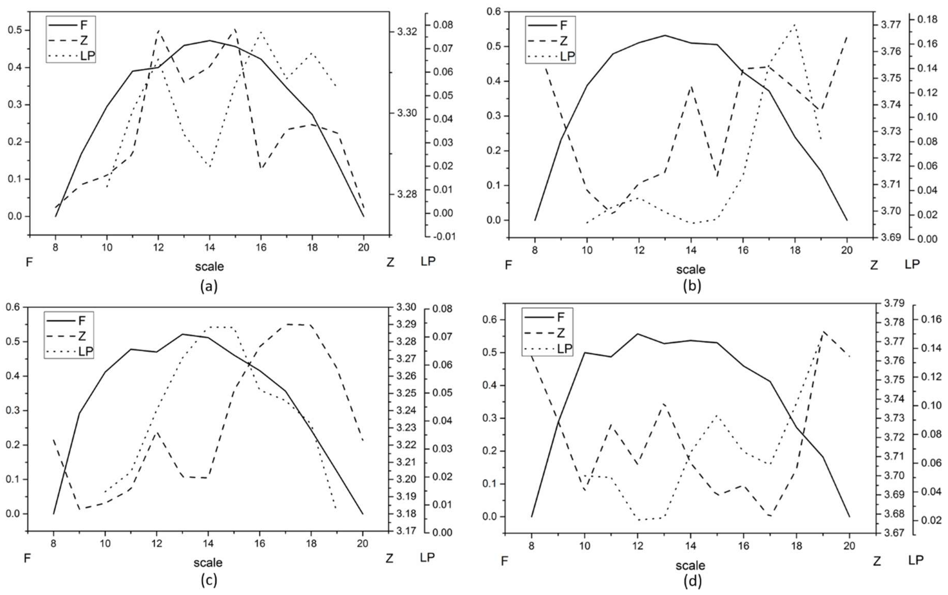
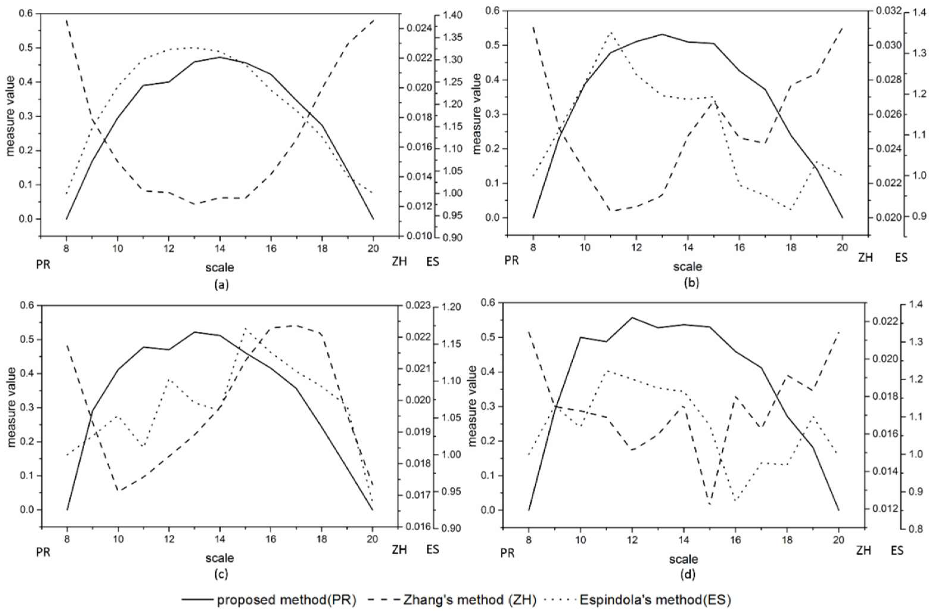
The combined measures of the F-measure, Z and LP methods are plotted as curves in Figure 6 for each test image. As illustrated in Section 2.3, the larger F-measure and LP values and the lower Z value indicate higher segmentation quality. For the T1 image, the best segmentation using the F-measure, Z, and LP methods was obtained by setting the scale at 14, 20, and 16, respectively (Figure 6a). For the T2 image, the best segmentation was obtained by setting the scale at 13, 11, and 18, respectively (Figure 6b). For the T3 image, the best segmentation was obtained by setting the scale at 13, 9, and 14, respectively (Figure 6c). For the T4 image, the best segmentation was obtained by setting the scale at 12, 17, and 19, respectively (Figure 6d). In general, the F-measure shows significant difference regarding the indications from the other two measures. The F-measure can clearly reveal the change in the segmentation quality when setting different scales for the MRS. When the image is over-segmented or under-segmented, the F-measure value is always low. From over-segmentation to under-segmentation, the F-measure shows the trend of first increasing and then decreasing, whereas the changing direction of Z and LP values varies more often. Thus, the F-measure is more sensitive to over- and under-segmentation than the other two measures. Moreover, we found that the optimal scales obtained by the LP method are always large for the four test images, and so the method is likely to be biased to under-segmented results.
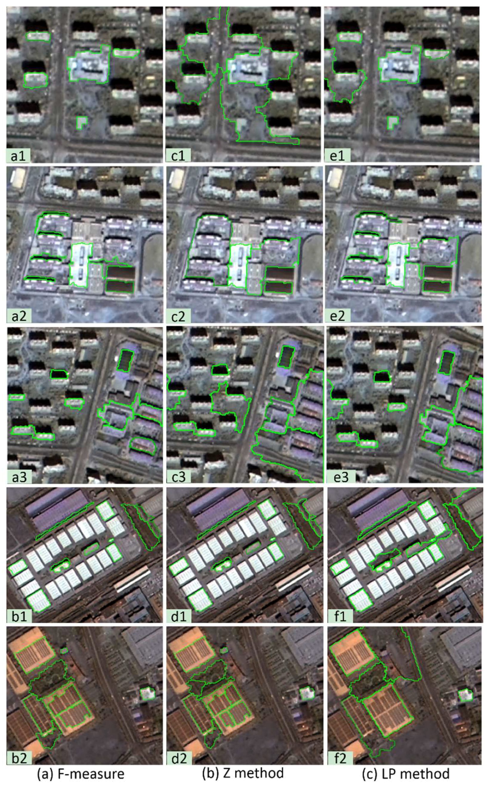
First, the best segmentation results produced by the MRS method for urban images of T1 and T2 using the optimal scales obtained by the F-measure, Z, and LP methods are presented in Figure 7. To further assess the segmentation quality, five subsets were selected from the T1 and T2 images to visually compare the best segmentation results using the optimal scales obtained by the three methods (Figure 8). Overall, the F-measure method was more accurate because it could allow the retrieval of the segmentation result, in which variously sized geo-objects were segmented well from a set of candidates (Figure 8a). By contrast, the other two methods obtained some over- or under-segmented geo-objects in their results (Figure 8b,c). In the first and third subsets, some buildings and impervious surfaces cannot be distinguished well in the Z and LP results. In the second subset, the shadow was under-segmented in the Z result, and the segmentations using the F-measure and LP method could discriminate the shadow well. However, the LP method obtained the under-segmented road in this subset. In the fourth subset, the shadow and some building were segmented out in the F-measure and Z results, whereas the LP method cannot obtain the segmentation that can distinguish the shadow and building very well. In the fifth subset, the large tree field was over-segmented in the Z result, and both a small building and a large building were under-segmented with other geo-objects in the LP result. However, the LP method was more accurate than the Z method in most cases.
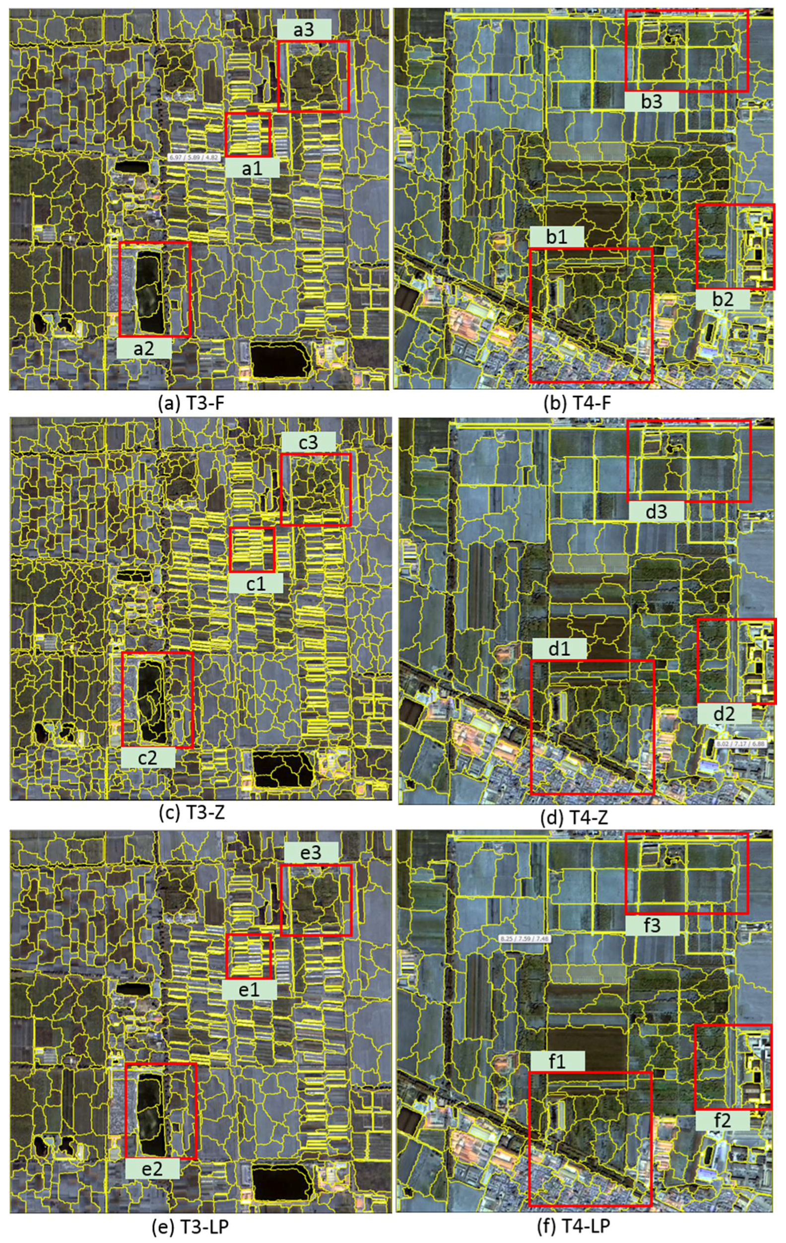
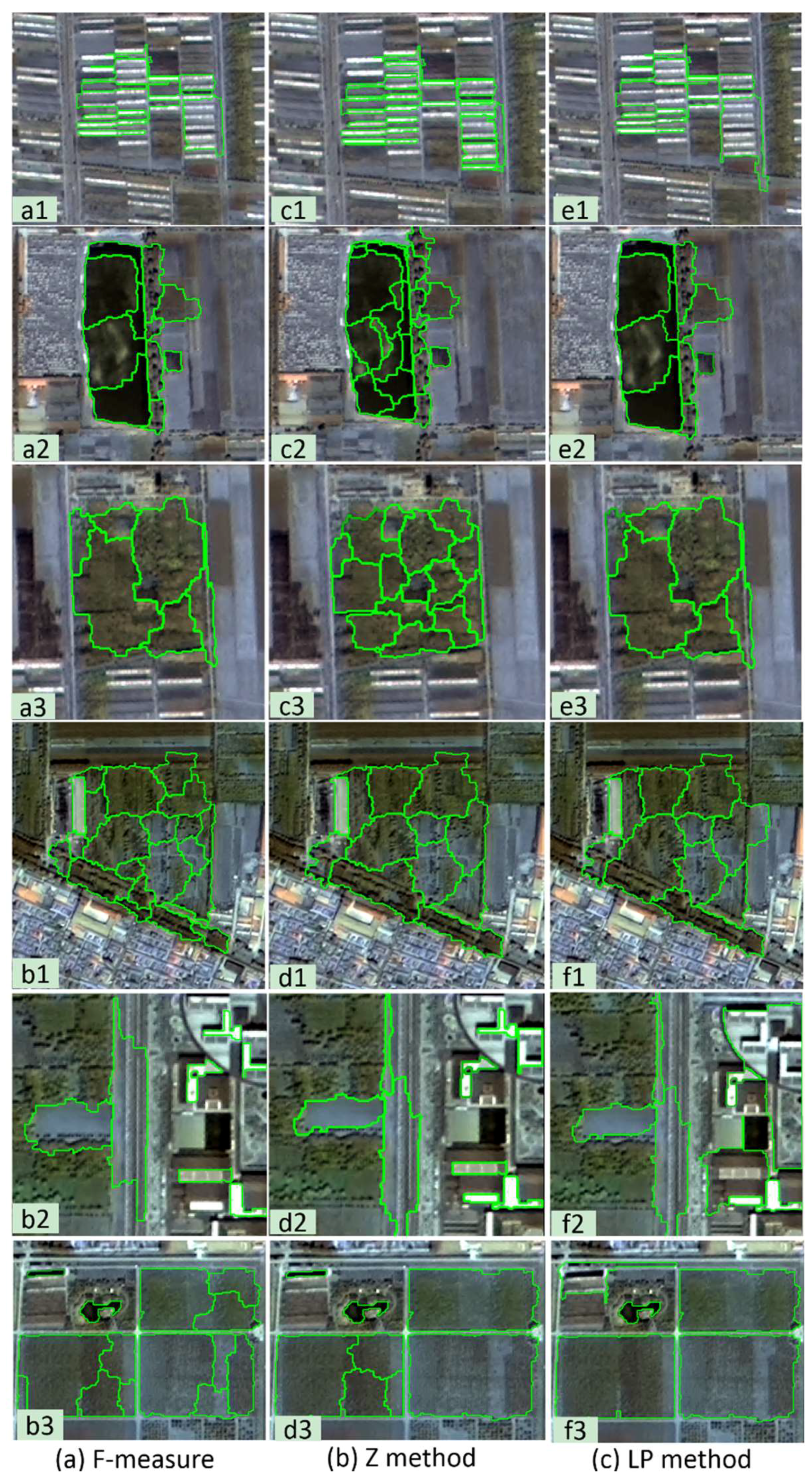
Second, we show the best segmentation results produced by the MRS method for the rural images of T3 and T4 using the optimal scales obtained by the three combination methods in Figure 9. Then, a close-up of six subsets selected from the T3 and T4 images in the segmentation results was used to demonstrate the differences (Figure 10). The segmentation results of the T3 and T4 images also demonstrated the fact that the F-measure could allow the obtaining of different sizes of geo-objects in its result (Figure 10a), whereas some geo-objects occurred in over- and under-segmentation in the Z and LP results (Figure 10b,c). In the first subset, the cultivation hothouses were segmented well in the Z result, but these areas were under-segmented in the F-measure and LP results. Moreover, the F-measure was more accurate than the LP method in this subset. The second subset showed the F-measure’s advantage. The tree cluster and water in this subset were separated from other geo-objects in their entirety by the F-measure, whereas there were bad performances in the Z and LP results, in which the tree cluster and water were over-segmented by the Z method, and the tree cluster was wrongly merged with the farmland by the LP method. In the third subset, the F-measure and LP method got nearly the same segmentations, but the tree cluster was over-segmented in the Z result. In the fifth and sixth subsets, the tree cluster and small buildings were segmented out in the F-measure result, whereas the tree cluster and mall buildings cannot be distinguished well in the other two methods’ results, respectively. However, the Z method had a better performance than the LP method in these two subsets. In the final subset, small geo-objects were segmented well in the F-measure and Z results, but large geo-objects were segmented well in the LP result. However, under-segmentation is a greater problem than over-segmentation, because it would largely affect the subsequent image analyses [32].
Finally, the SE results were presented to further demonstrate the effectiveness of the three combination methods (Table 1). In this paper, a total of 50 reference polygons were randomly delineated for each scene to calculate the SE accuracy metrics (Figure 3). For the T1, T3, and T4 images, the F-measure had lower QR and D values than the Z and LP methods, thus, indicating that the segmentations produced by the MRS method using the optimal scale obtained by the F-measure were the best in these three images. For the T2 image, the F-measure and Z method had almost the same lower QR and D values than the LP method, thus, indicating that they were better performers in the F-measure and Z results. In summary, the visual and quantitative results demonstrate that the F-measure is more accurate than the Z and LP methods.
3.4. Comparison with Existing UE Methods
The effectiveness of the combined indicators is further demonstrated by comparing them with Zhang et al. [23] and Espindola et al.s’ [36] methods. Because the combined F-measure indicator performs better than the Z and LP indicators in Section 3.3, only the F-measure is presented for comparison in this subsection. The scale parameters are set the same as those described in Section 2.6. The results of the three UE methods mentioned above are presented in Figure 11. For the T1 image, the best segmentation using the three UE methods was obtained by setting the scale at 14, 13, and 13, respectively (Figure 11a). For the T2 image, the best segmentation was obtained by setting the scale at 13, 11, and 11, respectively (Figure 11b). For the T3 image, the best segmentation was obtained by setting the scale at 13, 10, and 15, respectively (Figure 11c). For the T4 image, the best segmentation was obtained by setting the scale at 12, 15, and 11, respectively (Figure 11d). The change in the segmentation quality can be clearly revealed by using the three UE methods in the T1 image because the measure values of Espindola and the proposed methods are small and that of Zhang’s method is large when over- or under-segmented. However, in the other three test images, the changing direction of the Zhang and Espindola methods varies more often, whereas the proposed method has the same trend as the T1 image when changing the scale from 8 to 20. Thus, the proposed UE method is more sensitive to over- and under-segmentation than the other two UE methods.
Then, the SE results were shown to quantitatively demonstrate the effectiveness of the proposed UE method (Table 2). For the T1 image, the QR and D values of the Zhang and Espindola methods were both lower than those of the proposed method, thus, indicating that the proposed method had a bad performance in the T1 result. For the T2 image, the QR values of the Zhang and Espindola methods were lower than that of the proposed method, whereas the D value of the proposed method was lower than that of the Zhang and Espindola methods, thus, showing that the three UE methods had similar performances in the T2 result. For the T3 and T4 images, the proposed method had lower QR and D values than the Zhang and Espindola methods, thus, indicating that the proposed method had a better segmentation quality than the other two UE methods in the T3 and T4 results. The quantitative comparison results demonstrated that it is suitable to evaluate the segmentation results using the proposed UE method.
3.5. The Performance of the Proposed Method in Another Dataset
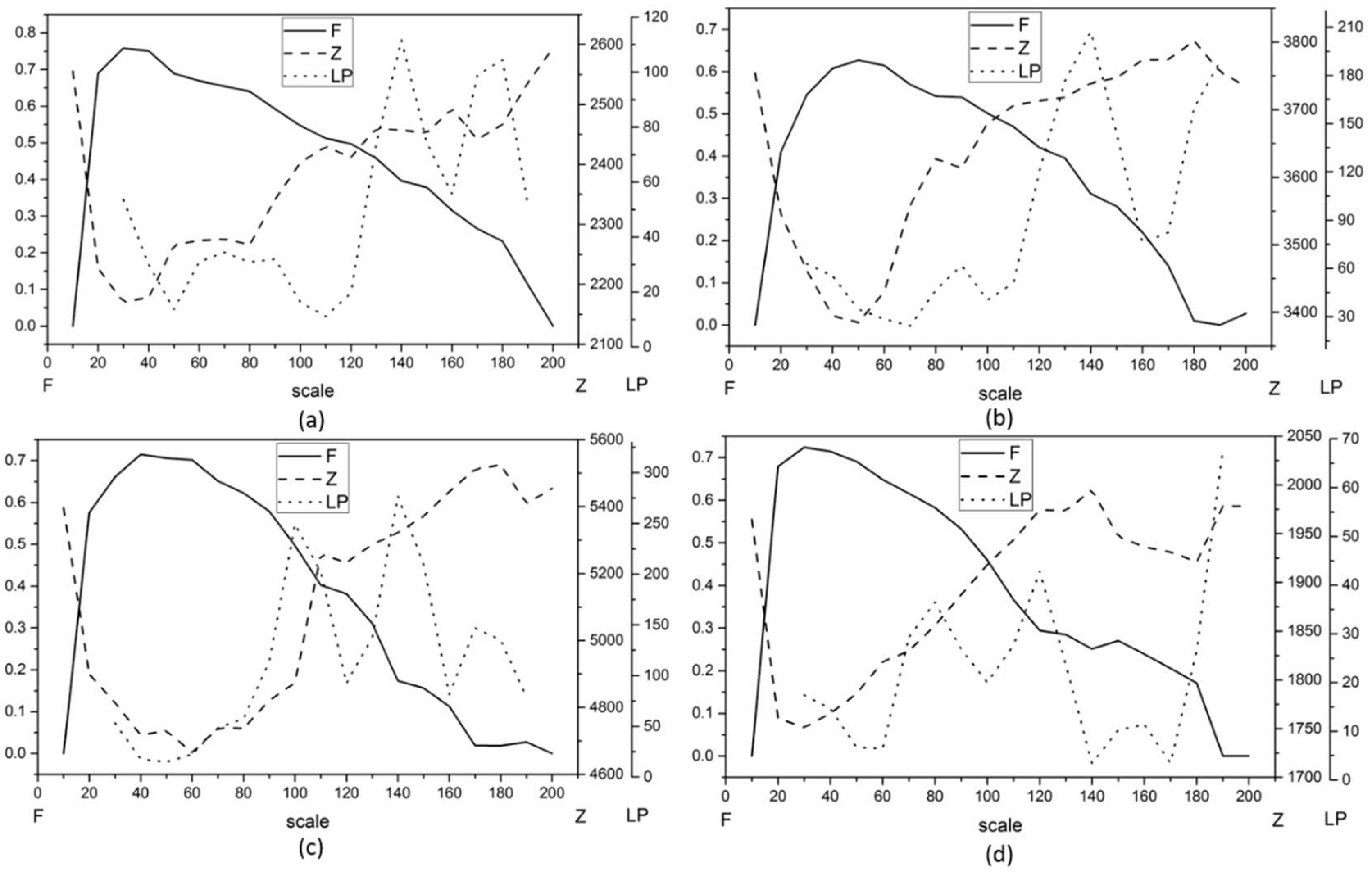
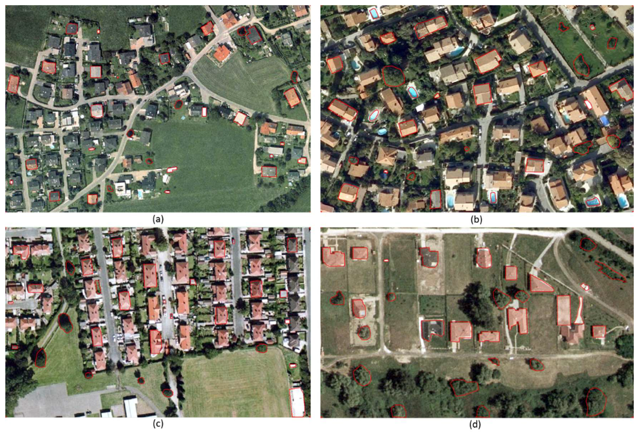
According to the experiments above, the proposed method showed good performance for improving segmentation quality in the GF-1 image applications. Furthermore, the SZTAKI-INRIA building detection dataset [48] is used to further evaluate the effectiveness of the proposed method, which was obtained from their website (http://web.eee.sztaki.hu/remotesensing/building_benchmark.html). Moreover, this dataset contains 9 aerial or satellite images taken from Budapest, Szada (both in Hungary), Manchester (UK), Bodensee (Germany), Normandy and Cot d’Azur (both in France). In this paper, images from the four regions of Bodensee, Cot d’Azur, Manchester and Szada were selected in the dataset. In this part, the scale was ranged from 10 to 200 in increments of 10, which was different from those for the GF-1 images. First, the three combination results of the WV and JM distance are shown in Figure 12. For the Bodensee image, the best segmentation using the F-measure, Z, and LP methods was obtained by setting the scale at 30, 200, and 140, respectively (Figure 12a). For the Cot d’Azur image, the best segmentation was obtained by setting the scale at 50, 180, and 140, respectively (Figure 12b). For the Manchester image, the best segmentation was obtained by setting the scale at 40, 180, and 140, respectively (Figure 12c). For the Szada image, the best segmentation was obtained by setting the scale at 30, 140, and 190, respectively (Figure 12d). Then, the SE results were shown to quantitatively demonstrate the effectiveness of the three combination strategies in the best segmentations (Table 3). In this paper, a total of 30 reference polygons were randomly delineated for each scene to calculate the SE accuracy metrics (Figure 13). For the four test images, the F-measure had the lowest QR and D values than the Z and LP methods, thus, indicating that the segmentations produced by the MRS method using the optimal scale obtained by the F-measure were the best in these four images. The quantitative results again demonstrate that the F-measure is more accurate than the Z and LP methods. Thus, the combination strategy of the F-measure was applied to the proposed method for the subsequent comparative analysis of the different UE methods.
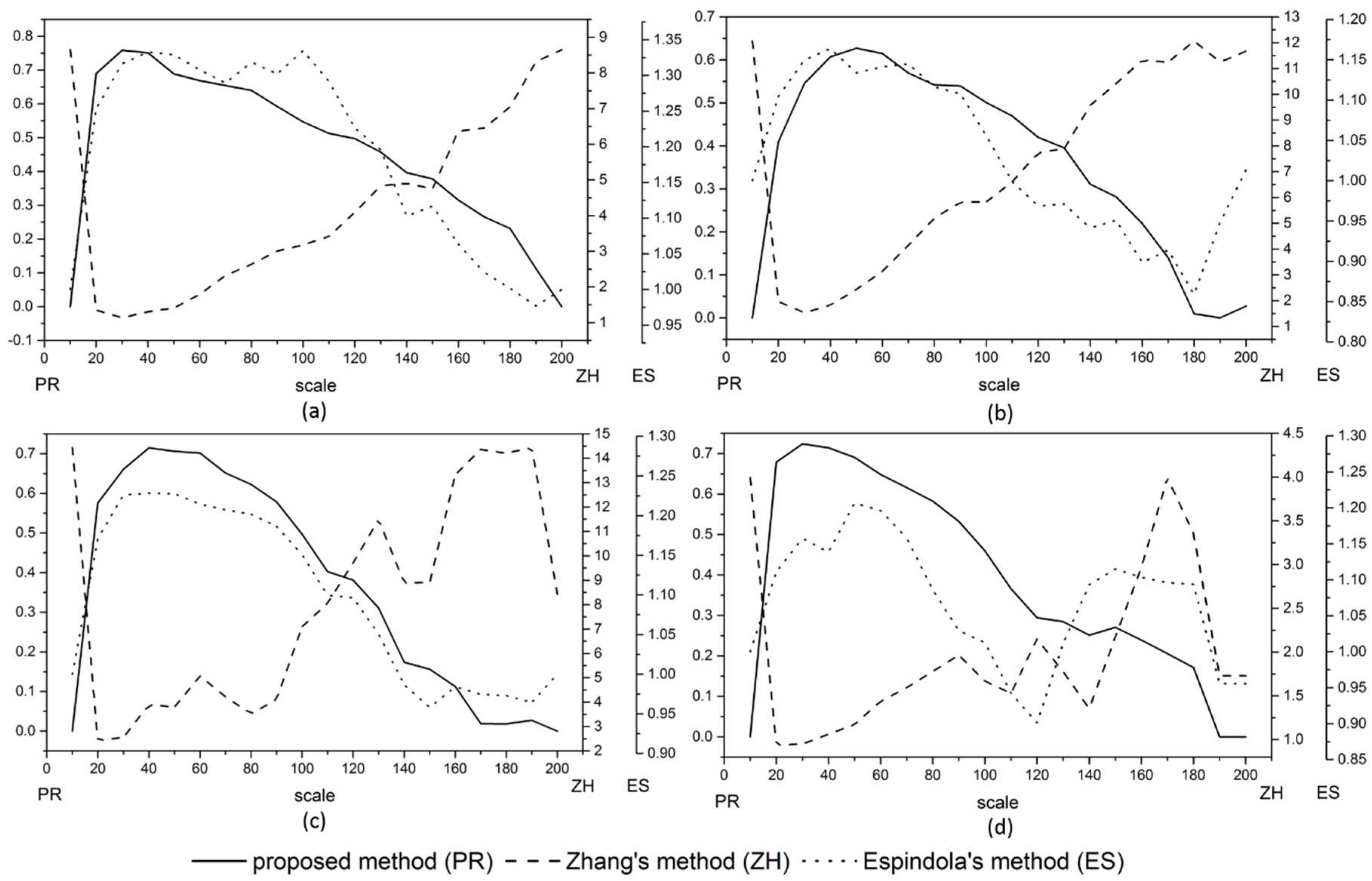
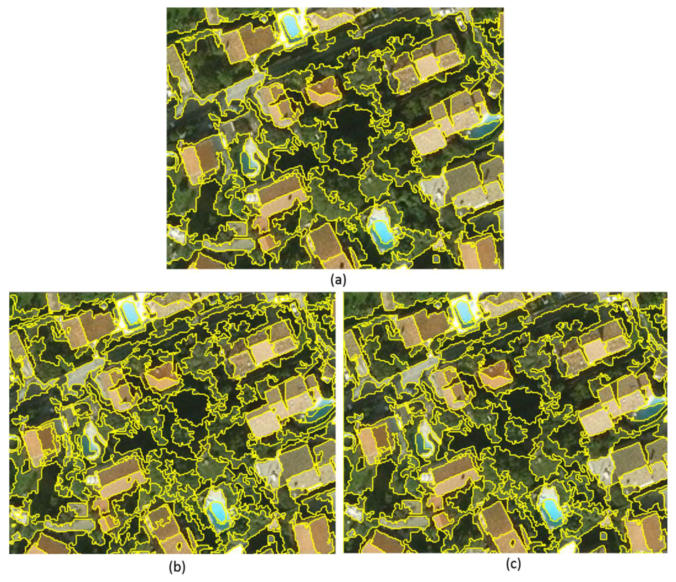
The three UE results of the proposed method and the Zhang and Espindola methods are presented in Figure 14. For the Bodensee image, the best segmentation using the three UE methods was obtained by setting the scale at 30, 30, and 100, respectively (Figure 14a). For the Cot d’Azur image, the best segmentation was obtained by setting the scale at 50, 30, and 40, respectively (Figure 14b). For the Manchester image, the best segmentation was obtained by setting the scale at 40, 20, and 40, respectively (Figure 14c). For the Manchester image, the best segmentation was obtained by setting the scale at 30, 20, and 50, respectively (Figure 14d). The best segmentations are shown in Figure 15 for visual comparison, where only the subsets of the Cot d’Azur results are presented. The SE results for the best segmentations with the optimal scale obtained by the three UE methods are shown in Table 4. The visual results showed that the proposed method had a better performance in allowing the obtaining of the best segmentations where the tree clusters could be segmented better than other two UE methods, whereas these three methods allowed the obtaining of a similar segmented building in the best segmentations. For the Bodensee, Cot d’Azur, and Manchester images, both the QR and D values of the proposed method were the lowest, thus, indicating that the proposed method had a better performance in allowing the retrieval of the segmentations with the high segmentation quality. However, for the Szada image, the Espindola method had the lowest QR and values, thus, showing the proposed method did not obtain the result with the best segmentation quality. Yet, the proposed method was more accurate than the Zhang method because it had lower QR and D values than the Zhang method. In summary, the visual and quantitative results proved that the proposed method could allowing the improvement of the segmentation quality in most cases.
4. Discussion
Image segmentation evaluation is a necessary prerequisite for obtaining a good segmentation result, and an accurate segmentation evaluation can improve the segmentation quality. Regardless of the visual analysis, the image segmentation evaluation can be categorized into the SE method and UE method. The SE method has an obvious advantage because it could provide a satisfactory characterization of geo-objects from the perspective of human interpretation. But it may be labor intensive and subjective for the user to manually digitize a large number of representative geo-objects in many applications [25]. At the moment, it cannot make the automation of selecting a proper scale for a given image. The UE method overcomes the aforementioned limitations and can make the automation of the scale parameterization more efficient and objective. In general, the intrasegment homogeneity and intersegment heterogeneity are considered in most UE methods and then are aggregated into a global value [27,29,37]. However, in the existing UE methods, the homogeneity measures are a local evaluation criteria, whereas the heterogeneity measures are a global evaluation criteria. This may cause a biased segmentation result because of the differences in the homogeneity and heterogeneity evaluation criteria characteristics. Moreover, the combination strategies for the homogeneity and heterogeneity measures must be carefully designed to achieve the potential trade-offs of different measures. Different combination strategies can lead to allowing for the retrieval of different segmentations. To address the issue mentioned above, the proposed UE method combines the WV and JM distance into a global value, in which the two measures are both local evaluation criteria, to evaluate the segmentation result. Then the contribution of the common border between adjacent segments and the area of each segment were integrated into the JM distance formula to make the heterogeneity measure more effective and objective. In addition, the three combination strategies of the F-measure, Z and LP methods were compared and analyzed to achieve the potential trade-offs of different measures. This proposed method provides a possible solution to obtain a more efficient and objective segmentation evaluation result by establishing the consistency of the homogeneity and heterogeneity criteria characteristics.
The proposed UE method focuses on the scale parameterization, which is the most important process for the characterization of real geo-objects. The scale parameterization is a generalized definition of the parameter that controls the sizes of image segments, and the sizes are adjusted by increasing or decreasing the corresponding parameter in the segmentation process [32]. Thus, the proposed UE method is believed to be transferable when employing different algorithms to segment images. As aforementioned, segmentation results impact the subsequent GEOBIA performance. It is an accepted fact that higher segmentation quality would improve the classification accuracy, but it is not always intuitive for the relationship between segmentation quality and classification accuracy. Over-segmentation may lead to a better classification when the spectral features are distinct, because it could classify smaller patches of land covers. However, the function of image segmentation is to recognize real geo-objects rather than classification, and, thus, it should be independent upon the classification.
The proposed UE method is a single-scale segmentation scale optimization technology. However, the fact often occurs that there are many different geo-object sizes, such as factories, farmland, water and tree clusters, in an image (Figure 3). In many cases, multiple scales should be used jointly for image analysis because representing the various objects in high spatial resolution images using a single segmentation is difficult. For SE methods, it is easy to evaluate multi-scale segmentations by preparing different groups of reference objects at multiple scales. However, it is difficult to evaluate multi-scale segmentations using UE methods, because the UE methods evaluate the segmentation quality based on the intrasegment homogeneity and intersegment heterogeneity criteria. A possible solution is to build the correspondence between the evaluation criteria and the semantic meaning of geo-objects. For example, in a farmland image (Figure 3d), we can imagine a layered segmentation in which one segment is occupied by a big field in low resolution, and one segment is crossed by a road in high resolution. Then, we could introduce hierarchical analysis and establish a link with different analysis layers as future work.
The WV and JM distance measures are jointly used to evaluate the segmentation quality. The proposed measures are sensitive to both over- and under-segmentation. In the case of over-segmentation, the WV value is small and the JM value is large. When under-segmented, the two measure values are inverse compared to over-segmentation. The curve is plotted on a set of multi-scale segmentations, which clearly reflects the change from over- to under-segmentation (Figure 4). In general, the WV value increases and the JM value decreases as the segmentation scale coarsens, thus, demonstrating the effectiveness of the proposed measures.
When comparing two segmentation results, if one segmentation has lower values regarding both measures than the other, its quality will be higher than that of the other. However, it is common that the two measures of one segmentation do not concurrently have higher or lower values than those of another segmentation. To solve the complexity, in this paper, the WV and JM distance measures are combined using three different methods to indicate the segmentation quality and to capture the trade-off between the two measures. The study of Zhang [4] has shown that the F-measure is more effective for combining the within and between-segment heterogeneity metrics and can penalize excessive under- or over-segmentation when compared to the sum and Euclidean distance (including ED and ED’) combination strategies, and, thus, this paper compared the three combination strategies of the F-measure, Z, and LP methods. The visual and quantitative SE results (Figure 8 and Figure 10, and Table 1) show that the F-measure performs better than both the Z and LP methods, which is a similar conclusion to Zhang. The combination strategies are applied to the same WV and JM values, thus, proving the superiority of F-measure. To further demonstrate the effectiveness of the proposed UE method, this paper compared it to the Zhang [23] and Espindola [36] methods. The quantitative SE results (Table 2) in the T1 and T2 images indicate that the proposed method was not always more accurate than the Zhang and Espindola methods, thus, showing that further improving the UE methods using other metrics is possible. But in the quantitative SE results of the T3 and T4 images, both the QR and D values of the proposed method were lower than those of the Zhang and Espindola methods, which indicates that the proposed method performed better than the other two methods. The experiments in the SZTAKI-INRIA building detection dataset again demonstrate that the proposed UE method had a good performance in allowing the retrieval of the results with high segmentation quality.
The main contributions of this study are as follows: (1) The existing UE methods use different evaluation criteria characteristics to express the intrasegment homogeneity and intersegment heterogeneity, thus, limiting the goodness-of-fit between segments and geo-objects. This is because the difference in the homogeneity and heterogeneity evaluation criteria characteristics may cause a biased segmentation result, i.e., an over- or under-segmented result. To overcome this limitation, this paper proposed a UE method using the WV and JM distance, which are both local measure criteria, to express the homogeneity and heterogeneity. (2) This paper considered the contribution of the common border between adjacent segments and the area of each segment in the JM distance formula, thus, making the heterogeneity measure more effective and objective. (3) This paper first compared the segmentation results using the three different combination strategies of the F-measure, Z, and LP methods, and the results demonstrate that the F-measure is more accurate than the other two combination strategies. Then, the F-measure was applied to the proposed method to be compared with the Zhang and Espindola methods. The visual and quantitative SE results show that the proposed method has a good performance in allowing the obtaining of the result with high segmentation quality, demonstrating the superiority of using the same evaluation criteria characteristic in the proposed UE method.
5. Conclusions
A UE method of the WV and JM distance measures based on local measure criteria has been proposed for evaluating segmentation quality, and the JM distance is improved by considering the contribution of the common border between adjacent segments and the area of each segment to make the heterogeneity measure more effective and objective. The two measures are jointly used to reveal the segmentation quality by changing the scale from 8 to 20. Then, to clearly indicate the segmentation quality, the three combination strategies of the F-measure, Z, and LP methods are compared and evaluated according to the visual analysis and the SE methods of quality rate (QR), under-segmentation (US), over-segmentation (OS), and an index of combining the US and OS (D). Finally, the proposed UE method is compared with the Zhang and Espindola methods to further demonstrate the effectiveness of the proposed UE method. The MRS method embedded in eCognition Developer 8.7 is adopted for the evaluation. A GF-1 image is used as an example, and a set of images of different study areas was used to perform the experiments to show the effectiveness of the proposed measures. The experimental results show that the WV and JM distance measures can reflect the change in image quality during a coarsening of the segmentation scales for the MRS, demonstrating the superiority of the local evaluation criteria in the proposed UE method. The combined strategy of the F-measure can clearly reveal the segmentation quality when different scales are set. The effectiveness of the combined indicator is further proven by comparing it with two existing UE methods. The visual and quantitative SE results prove that the proposed UE method can improve the segmentation quality. In the future, we will focus on building the correspondence between the evaluation criteria and the semantic meaning of geo-objects to satisfy multiple-scale image analysis for a given application and the combination of homogeneity and heterogeneity using other metrics to further improve the UE method’s performances.
Author Contributions
Conceptualization, Y.W. and Q.Q.; Data curation, Y.L.; Funding acquisition, Q.Q.; Investigation, Y.W. and Y.L.; Methodology, Y.W.; Supervision, Q.Q.; Validation, Y.W. and Y.L.; Visualization, Y.W.; Writing—original draft, Y.W.; Writing—review and editing, Y.W., Q.Q. and Y.L.
Funding
This study was supported by the Science and Technology Service Network Project with project number KFJ-EW-STS-069, and the Special Topic of Basic Work of Science and Technology with project number 2007FY140800.
Acknowledgments
Thanks to Csaba Benedek for supplying the SZTAKI-INRIA building detection dataset as parts of experimental data for this study. The authors would like to thank the reviewers and editors for the comments and suggestions.
Conflicts of Interest
The authors declare no conflicts of interest.
References
- Blaschke, T. Object based image analysis for remote sensing. ISPRS J. Photogramm. Remote Sens. 2010, 65, 2–16. [Google Scholar] [CrossRef]
- Blaschke, T.; Hay, G.J.; Kelly, M.; Lang, S.; Hofmann, P.; Addink, E.; Feitosa, R.Q.; van der Meer, F.; van der Werff, H.; van Coillie, F.; et al. Geographic object-based image analysis—Towards a new paradigm. ISPRS J. Photogramm. Remote Sens. 2014, 87, 180–191. [Google Scholar] [CrossRef] [PubMed]
- Hay, G.J.; Castilla, G.; Wulder, M.A.; Ruiz, J.R. An automated object-based approach for the multiscale image segmentation of forest scenes. Int. J. Appl. Earth Obs. Geoinf. 2005, 7, 339–359. [Google Scholar] [CrossRef]
- Zhang, X.L.; Feng, X.Z.; Xiao, P.F.; He, G.J.; Zhu, L.J. Segmentation quality evaluation using region-based precision and recall measures for remote sensing images. ISPRS J. Photogramm. Remote Sens. 2015, 102, 73–84. [Google Scholar] [CrossRef]
- Zhang, X.L.; Xiao, P.F.; Feng, X.Z.; Wang, J.G.; Wang, Z. Hybrid region merging method for segmentation of high-resolution remote sensing images. ISPRS J. Photogramm. Remote Sens. 2014, 98, 19–28. [Google Scholar] [CrossRef]
- Myint, S.W.; Gober, P.; Brazel, A.; Grossman-Clarke, S.; Weng, Q.H. Per-pixel vs. Object-based classification of urban land cover extraction using high spatial resolution imagery. Remote Sens. Environ. 2011, 115, 1145–1161. [Google Scholar] [CrossRef]
- Su, T.F.; Zhang, S.W. Local and global evaluation for remote sensing image segmentation. ISPRS J. Photogramm. Remote Sens. 2017, 130, 256–276. [Google Scholar] [CrossRef]
- Yang, J.; He, Y.H.; Caspersen, J.; Jones, T. A discrepancy measure for segmentation evaluation from the perspective of object recognition. ISPRS J. Photogramm. Remote Sens. 2015, 101, 186–192. [Google Scholar] [CrossRef]
- Pekkarinen, A. A method for the segmentation of very high spatial resolution images of forested landscapes. Int. J. Remote Sens. 2002, 23, 2817–2836. [Google Scholar] [CrossRef]
- Chen, L.C.; Papandreou, G.; Kokkinos, I.; Murphy, K.; Yuille, A.L. Deeplab: Semantic image segmentation with deep convolutional nets, atrous convolution, and fully connected crfs. IEEE Trans. Pattern Anal. Mach. Intell. 2018, 40, 834–848. [Google Scholar] [CrossRef] [PubMed]
- Happ, P.N.; Ferreira, R.S.; Bentes, C.; Costa, G.; Feitosa, R.Q. Multiresolution segmentation: A parallel approach for high resolution image segmentation in multicore architectures. In Int Arch Photogramm; Addink, E.A., VanCoillie, F.M.B., Eds.; Copernicus Gesellschaft Mbh: Gottingen, German, 2010; PP 38-4-C7. [Google Scholar]
- Doulamis, A.D.; Doulamis, N.D.; Kollias, S.D. A fuzzy video content representation for video summarization and content-based retrieval. Signal Process. 2000, 80, 1049–1067. [Google Scholar] [CrossRef] [Green Version]
- Vincent, L.; Soille, P. Watersheds in digital spaces—An efficient algorithm based on immersion simulations. IEEE Trans. Pattern Anal. Mach. Intell. 1991, 13, 583–598. [Google Scholar] [CrossRef]
- Wagner, B.; Dinges, A.; Muller, P.; Haase, G. Parallel volume image segmentation with watershed transformation. Lect. Notes Comput. Sci. 2009, 5575, 420–429. [Google Scholar]
- Shi, J.B.; Malik, J. Normalized cuts and image segmentation. IEEE Trans. Pattern Anal. Mach. Intell. 2000, 22, 888–905. [Google Scholar] [Green Version]
- Benz, U.C.; Hofmann, P.; Willhauck, G.; Lingenfelder, I.; Heynen, M. Multi-resolution, object-oriented fuzzy analysis of remote sensing data for gis-ready information. ISPRS J. Photogramm. Remote Sens. 2004, 58, 239–258. [Google Scholar] [CrossRef]
- Böck, S.; Immitzer, M.; Atzberger, C. On the objectivity of the objective function—Problems with unsupervised segmentation evaluation based on global score and a possible remedy. Remote Sens. 2017, 9, 769. [Google Scholar] [CrossRef]
- Cardoso, J.S.; Corte-Real, L. Toward a generic evaluation of image segmentation. IEEE Trans. Image Process. 2005, 14, 1773–1782. [Google Scholar] [CrossRef] [PubMed] [Green Version]
- Clinton, N.; Holt, A.; Scarborough, J.; Yan, L.; Gong, P. Accuracy assessment measures for object-based image segmentation goodness. Photogramm. Eng. Remote Sens. 2010, 76, 289–299. [Google Scholar] [CrossRef]
- Dragut, L.; Csillik, O.; Eisank, C.; Tiede, D. Automated parameterisation for multi-scale image segmentation on multiple layers. ISPRS J. Photogramm. Remote Sens. 2014, 88, 119–127. [Google Scholar] [CrossRef] [PubMed]
- Johnson, B.A.; Bragais, M.; Endo, I.; Magcale-Macandog, D.B.; Macandog, P.B.M. Image segmentation parameter optimization considering within- and between-segment heterogeneity at multiple scale levels: Test case for mapping residential areas using landsat imagery. ISPRS Int. Geo-Inf. 2015, 4, 2292–2305. [Google Scholar] [CrossRef]
- Grybas, H.; Melendy, L.; Congalton, R.G. A comparison of unsupervised segmentation parameter optimization approaches using moderate- and high-resolution imagery. Gisci. Remote Sens. 2017, 54, 515–533. [Google Scholar] [CrossRef]
- Zhang, X.L.; Xiao, P.F.; Feng, X.Z. An unsupervised evaluation method for remotely sensed imagery segmentation. IEEE Geosci. Remote Sens. Lett. 2012, 9, 156–160. [Google Scholar] [CrossRef]
- Johnson, B.; Xie, Z.X. Unsupervised image segmentation evaluation and refinement using a multi-scale approach. ISPRS J. Photogramm. Remote Sens. 2011, 66, 473–483. [Google Scholar] [CrossRef]
- Zhang, H.; Fritts, J.E.; Goldman, S.A. Image segmentation evaluation: A survey of unsupervised methods. Comput. Vis. Image Understand. 2008, 110, 260–280. [Google Scholar] [CrossRef] [Green Version]
- Flanders, D.; Hall-Beyer, M.; Pereverzoff, J. Preliminary evaluation of ecognition object-based software for cut block delineation and feature extraction. Can. J. Remote Sens. 2003, 29, 441–452. [Google Scholar] [CrossRef]
- Duro, D.C.; Franklin, S.E.; Dube, M.G. A comparison of pixel-based and object-based image analysis with selected machine learning algorithms for the classification of agricultural landscapes using spot-5 hrg imagery. Remote Sens. Environ. 2012, 118, 259–272. [Google Scholar] [CrossRef]
- Liu, Y.; Bian, L.; Meng, Y.H.; Wang, H.P.; Zhang, S.F.; Yang, Y.N.; Shao, X.M.; Wang, B. Discrepancy measures for selecting optimal combination of parameter values in object-based image analysis. ISPRS J. Photogramm. Remote Sens. 2012, 68, 144–156. [Google Scholar] [CrossRef]
- Yang, J.; Li, P.J.; He, Y.H. A multi-band approach to unsupervised scale parameter selection for multi-scale image segmentation. ISPRS J. Photogramm. Remote Sens. 2014, 94, 13–24. [Google Scholar] [CrossRef]
- Zhang, X.L.; Xiao, P.F.; Song, X.Q.; She, J.F. Boundary-constrained multi-scale segmentation method for remote sensing images. ISPRS J. Photogramm. Remote Sens. 2013, 78, 15–25. [Google Scholar] [CrossRef]
- Abeyta, A.M.; Franklin, J. The accuracy of vegetation stand boundaries derived from image segmentation in a desert environment. Photogramm. Eng. Remote Sens. 1998, 64, 59–66. [Google Scholar]
- Yang, J.; He, Y.H.; Weng, Q.H. An automated method to parameterize segmentation scale by enhancing intrasegment homogeneity and intersegment heterogeneity. IEEE Geosci. Remote Sens. Lett. 2015, 12, 1282–1286. [Google Scholar] [CrossRef]
- Dragut, L.; Tiede, D.; Levick, S.R. Esp: A tool to estimate scale parameter for multiresolution image segmentation of remotely sensed data. Int. J. Geogr. Inf. Sci. 2010, 24, 859–871. [Google Scholar] [CrossRef]
- Kim, M.; Madden, M.; Warner, T. Estimation of Optimal Image Object Size for the Segmentation of Forest Stands with Multispectral Ikonos Imagery; Springer: Berlin/Heidelberg, Germany, 2008; pp. 291–307. [Google Scholar]
- Chabrier, S.; Emile, B.; Rosenberger, C.; Laurent, H. Unsupervised performance evaluation of image segmentation. EURASIP J. Appl. Signal Process. 2006, 2006, 96306. [Google Scholar] [CrossRef]
- Espindola, G.M.; Camara, G.; Reis, I.A.; Bins, L.S.; Monteiro, A.M. Parameter selection for region-growing image segmentation algorithms using spatial autocorrelation. Int. J. Remote Sens. 2006, 27, 3035–3040. [Google Scholar] [CrossRef]
- Kim, M.; Madden, M.; Warner, T.A. Forest type mapping using object-specific texture measures from multispectral ikonos imagery: Segmentation quality and image classification issues. Photogramm. Eng. Remote Sens. 2009, 75, 819–829. [Google Scholar] [CrossRef]
- Faur, D.; Gavat, I.; Datcu, M. Salient remote sensing image segmentation based on rate-distortion measure. IEEE Geosci. Remote Sens. Lett. 2009, 6, 855–859. [Google Scholar] [CrossRef]
- Corcoran, P.; Winstanley, A.; Mooney, P. Segmentation performance evaluation for object-based remotely sensed image analysis. Int. J. Remote Sens. 2010, 31, 617–645. [Google Scholar] [CrossRef] [Green Version]
- Tremeau, A.; Colantoni, P. Regions adjacency graph applied to color image segmentation. IEEE Trans. Image Process. 2000, 9, 735–744. [Google Scholar] [CrossRef] [PubMed] [Green Version]
- Haris, K.; Efstratiadis, S.N.; Maglaveras, N.; Katsaggelos, A.K. Hybrid image segmentation using watersheds and fast region merging. IEEE Trans. Image Process. 1998, 7, 1684–1699. [Google Scholar] [CrossRef] [PubMed] [Green Version]
- Richards, J.A. Remote Sensing Digital Image Analysis: An Introduction; Springer: Berlin/Heidelberg, Germany, 2006; pp. 47–54. [Google Scholar]
- Schmidt, K.S.; Skidmore, A.K. Spectral discrimination of vegetation types in a coastal wetland. Remote Sens. Environ. 2003, 85, 92–108. [Google Scholar] [CrossRef]
- Leonardis, A.; Gupta, A.; Bajcsy, R. Segmentation of range images as the search for geometric parametric models. Int. J. Comput. Vis. 1995, 14, 253–277. [Google Scholar] [CrossRef]
- Hong, T.H.; Rosenfeld, A. Compact region extraction using weighted pixel linking in a pyramid. IEEE Trans. Pattern Anal. Mach. Intell. 1984, 6, 222–229. [Google Scholar] [CrossRef] [PubMed]
- Wang, Y.; Meng, Q.; Qi, Q.; Yang, J.; Liu, Y. Region merging considering within- and between-segment heterogeneity: An improved hybrid remote-sensing image segmentation method. Remote Sens. 2018, 10, 781. [Google Scholar] [CrossRef]
- Baatz, M.; Schape, A. Multiresolution Segmentation—An Optimization Approach for High Quality Multi-Scale Image Segmentation. In Angewandte Geographische Informations-Verarbeitung; Strobl, J., Blaschke, T., Griesebner, G., Eds.; Wichmanm Verlag: Karlsruhe, Germany, 2000; pp. 12–23. [Google Scholar]
- Benedek, C.; Descombes, X.; Zerubia, J. Building development monitoring in multitemporal remotely sensed image pairs with stochastic birth-death dynamics. IEEE Trans. Pattern Anal. Mach. Intell. 2012, 34, 33–50. [Google Scholar] [CrossRef] [PubMed] [Green Version]
Figure 1.
Schematic of calculating the area-weighted variance (WV) and Jeffries-Matusita (JM) distance measures to evaluate the segmentation quality.
Figure 1.
Schematic of calculating the area-weighted variance (WV) and Jeffries-Matusita (JM) distance measures to evaluate the segmentation quality.

Figure 2.
Sample illustrations of JM distance measure: (a) Segment1 is occupied by the pixel values of 1 and 2, and Segment2 is occupied by the pixel values of 5 and 6; (b) Segment1’ in which pixel value 3 is merged into Segment1; and (c) Segment1in which pixel value 4 is merged into Segment1’.
Figure 2.
Sample illustrations of JM distance measure: (a) Segment1 is occupied by the pixel values of 1 and 2, and Segment2 is occupied by the pixel values of 5 and 6; (b) Segment1’ in which pixel value 3 is merged into Segment1; and (c) Segment1in which pixel value 4 is merged into Segment1’.

Figure 3.
Four study areas of the gaofen-1 (GF-1) image: (a) T1, residential area, (b) T2, industrial area, (c) T3, farmland area includes vegetation, farmland, water, and a cultivation hothouse, and (d) T4, farmland area includes a forest, farmland, and a village. Red polygons represent the manually digitized reference objects.

Figure 4.
The WV and JM values of the segmentation results, produced by multiresolution segmentation (MRS) method with the scale from 8 to 20, for the four study areas of (a) T1, (b) T2, (c) T3, and (d)T4.
Figure 4.
The WV and JM values of the segmentation results, produced by multiresolution segmentation (MRS) method with the scale from 8 to 20, for the four study areas of (a) T1, (b) T2, (c) T3, and (d)T4.

Figure 5.
Subsets of segmenting four study areas: (a–d) are the segmentations of T1, T2, T3, and T4 produced by MRS with setting scale as 8, and (e–h) are the ones of T1, T2, T3, and T4 produced by MRS with setting scale as 20, respectively.
Figure 5.
Subsets of segmenting four study areas: (a–d) are the segmentations of T1, T2, T3, and T4 produced by MRS with setting scale as 8, and (e–h) are the ones of T1, T2, T3, and T4 produced by MRS with setting scale as 20, respectively.

Figure 6.
The unsupervised evaluation (UE) results of segmentations produced by the MRS method with a scale of 8–20 for the four study areas: (a) T1, (b) T2, (c) T3, and (d) T4.
Figure 6.
The unsupervised evaluation (UE) results of segmentations produced by the MRS method with a scale of 8–20 for the four study areas: (a) T1, (b) T2, (c) T3, and (d) T4.

Figure 7.
The segmentation results of the test images T1 and T2 produced by the MRS method with the optimal scales obtained by the three combination methods.
Figure 7.
The segmentation results of the test images T1 and T2 produced by the MRS method with the optimal scales obtained by the three combination methods.

Figure 8.
Subsets of the segmentation results in Figure 7, which are the F-measure, Z and LP results from left to right.
Figure 8.
Subsets of the segmentation results in Figure 7, which are the F-measure, Z and LP results from left to right.

Figure 9.
The segmentation results of the test images T3 and T4 produced by the MRS method with optimal scales obtained by the three combination methods.
Figure 9.
The segmentation results of the test images T3 and T4 produced by the MRS method with optimal scales obtained by the three combination methods.

Figure 10.
Subsets of the segmentation results in Figure 9, which are the F-measure, Z, and LP results from left to right.
Figure 10.
Subsets of the segmentation results in Figure 9, which are the F-measure, Z, and LP results from left to right.

Figure 11.
The UE results of the segmentations produced by the MRS method with the different UE methods for the four study areas: (a) T1, (b) T2, (c) T3, and (d) T4.
Figure 11.
The UE results of the segmentations produced by the MRS method with the different UE methods for the four study areas: (a) T1, (b) T2, (c) T3, and (d) T4.

Figure 12.
The UE results of the segmentations produced by the MRS method with different combination methods, using the SZTAKI-INRIA building detection dataset: (a) Bodensee, (b) Cot d’Azur, (c) Manchester, and (d) Szada.
Figure 12.
The UE results of the segmentations produced by the MRS method with different combination methods, using the SZTAKI-INRIA building detection dataset: (a) Bodensee, (b) Cot d’Azur, (c) Manchester, and (d) Szada.

Figure 13.
Referenced images using human interpretation, containing 30 regions in each image: (a) Bodensee, (b) Cot d’Azur, (c) Manchester, and (d) Szada. The red polygons represent the manually digitized reference objects.
Figure 13.
Referenced images using human interpretation, containing 30 regions in each image: (a) Bodensee, (b) Cot d’Azur, (c) Manchester, and (d) Szada. The red polygons represent the manually digitized reference objects.

Figure 14.
The UE results of the segmentations produced by the MRS method with different UE methods, using the SZTAKI-INRIA building detection dataset: (a) Bodensee, (b) Cot d’Azur, (c) Manchester, and (d) Szada.
Figure 14.
The UE results of the segmentations produced by the MRS method with different UE methods, using the SZTAKI-INRIA building detection dataset: (a) Bodensee, (b) Cot d’Azur, (c) Manchester, and (d) Szada.

Figure 15.
Subsets of the segmentation results with the optimal scale obtained by different UE methods: (a) proposed method, (b) Zhang method and (c) Espindola method.
Figure 15.
Subsets of the segmentation results with the optimal scale obtained by different UE methods: (a) proposed method, (b) Zhang method and (c) Espindola method.


Table 1.
The supervised evaluation (SE) results for the segmentations produced with the three combination methods.
Table 1.
The supervised evaluation (SE) results for the segmentations produced with the three combination methods.
| Test | Combination Methods | Segmentation Accuracy Metrics | |||
|---|---|---|---|---|---|
| QR | OS | US | D | ||
| T1 | F-measure | 0.4177 | 0.0963 | 0.3548 | 0.26 |
| Z method | 0.6121 | 0.0717 | 0.5673 | 0.4043 | |
| LP method | 0.4786 | 0.089 | 0.4166 | 0.3012 | |
| T2 | F-measure | 0.3052 | 0.1544 | 0.1679 | 0.1613 |
| Z method | 0.2972 | 0.1836 | 0.1355 | 0.1614 | |
| LP method | 0.4665 | 0.0643 | 0.423 | 0.3026 | |
| T3 | F-measure | 0.3995 | 0.162 | 0.2764 | 0.2265 |
| Z method | 0.4326 | 0.3088 | 0.1683 | 0.2487 | |
| LP method | 0.4124 | 0.1571 | 0.2942 | 0.2358 | |
| T4 | F-measure | 0.4637 | 0.1156 | 0.387 | 0.2856 |
| Z method | 0.5954 | 0.076 | 0.5609 | 0.4003 | |
| LP method | 0.6215 | 0.0455 | 0.6087 | 0.4316 | |
Table 2.
The supervised evaluation (SE) results for the segmentations produced with the different unsupervised evaluation (UE) methods.
Table 2.
The supervised evaluation (SE) results for the segmentations produced with the different unsupervised evaluation (UE) methods.
| Test | UE Methods | Segmentation Accuracy Metrics | |||
|---|---|---|---|---|---|
| QR | OS | US | D | ||
| T1 | Proposed method | 0.4177 | 0.0963 | 0.3548 | 0.26 |
| Zhang method | 0.4071 | 0.112 | 0.3331 | 0.2485 | |
| Espindola method | 0.4071 | 0.112 | 0.3331 | 0.2485 | |
| T2 | Proposed method | 0.3052 | 0.1544 | 0.1679 | 0.1613 |
| Zhang method | 0.2972 | 0.1836 | 0.1355 | 0.1614 | |
| Espindola method | 0.2972 | 0.1836 | 0.1355 | 0.1614 | |
| T3 | Proposed method | 0.3995 | 0.162 | 0.2764 | 0.2265 |
| Zhang method | 0.4129 | 0.2709 | 0.1856 | 0.2322 | |
| Espindola method | 0.4469 | 0.1635 | 0.3233 | 0.2562 | |
| T4 | Proposed method | 0.4637 | 0.1156 | 0.387 | 0.2856 |
| Zhang method | 0.545 | 0.0953 | 0.494 | 0.3558 | |
| Espindola method | 0.4796 | 0.1694 | 0.3669 | 0.2857 | |
Table 3.
The SE results for the segmentations produced with the three combination methods.
| Test | Combination Methods | Segmentation Accuracy Metrics | |||
|---|---|---|---|---|---|
| QR | OS | US | D | ||
| Bodensee | F-measure | 0.3797 | 0.2931 | 0.147 | 0.2318 |
| Z method | 0.7994 | 0.025 | 0.7895 | 0.5586 | |
| LP method | 0.693 | 0.0271 | 0.6795 | 0.4808 | |
| Cot d’Azur | F-measure | 0.5254 | 0.3838 | 0.2575 | 0.3268 |
| Z method | 0.8275 | 0.0754 | 0.8187 | 0.5813 | |
| LP method | 0.7846 | 0.1234 | 0.7526 | 0.5393 | |
| Manchester | F-measure | 0.5378 | 0.4033 | 0.2462 | 0.3341 |
| Z method | 0.8531 | 0.0995 | 0.8403 | 0.5983 | |
| LP method | 0.813 | 0.1018 | 0.7963 | 0.5676 | |
| Szada | F-measure | 0.5294 | 0.4794 | 0.1615 | 0.3577 |
| Z method | 0.6302 | 0.1223 | 0.5943 | 0.4291 | |
| LP method | 0.791 | 0.0609 | 0.7715 | 0.5472 | |
Table 4.
The SE results for the segmentations produced with the different UE methods, using the SZTAKI-INRIA building detection dataset.
Table 4.
The SE results for the segmentations produced with the different UE methods, using the SZTAKI-INRIA building detection dataset.
| Test | UE Methods | Segmentation Accuracy Metrics | |||
|---|---|---|---|---|---|
| QR | OS | US | D | ||
| Bodensee | Proposed method | 0.3797 | 0.2931 | 0.147 | 0.2318 |
| Zhang method | 0.3797 | 0.2931 | 0.147 | 0.2318 | |
| Espindola method | 0.5646 | 0.0746 | 0.521 | 0.3722 | |
| Cot d’Azur | Proposed method | 0.5254 | 0.3838 | 0.2575 | 0.3268 |
| Zhang method | 0.5416 | 0.4395 | 0.2206 | 0.3477 | |
| Espindola method | 0.5385 | 0.33 | 0.3276 | 0.3288 | |
| Manchester | Proposed method | 0.5378 | 0.4033 | 0.2462 | 0.3341 |
| Zhang method | 0.5842 | 0.5377 | 0.1183 | 0.3893 | |
| Espindola method | 0.5378 | 0.4033 | 0.2462 | 0.3341 | |
| Szada | Proposed method | 0.5294 | 0.4794 | 0.1615 | 0.3577 |
| Zhang method | 0.6122 | 0.5912 | 0.1016 | 0.4241 | |
| Espindola method | 0.503 | 0.3739 | 0.2866 | 0.3331 | |
© 2018 by the authors. Licensee MDPI, Basel, Switzerland. This article is an open access article distributed under the terms and conditions of the Creative Commons Attribution (CC BY) license (http://creativecommons.org/licenses/by/4.0/).
Share and Cite
MDPI and ACS Style
Wang, Y.; Qi, Q.; Liu, Y. Unsupervised Segmentation Evaluation Using Area-Weighted Variance and Jeffries-Matusita Distance for Remote Sensing Images. Remote Sens. 2018, 10, 1193. https://doi.org/10.3390/rs10081193
AMA Style
Wang Y, Qi Q, Liu Y. Unsupervised Segmentation Evaluation Using Area-Weighted Variance and Jeffries-Matusita Distance for Remote Sensing Images. Remote Sensing. 2018; 10(8):1193. https://doi.org/10.3390/rs10081193
Chicago/Turabian StyleWang, Yongji, Qingwen Qi, and Ying Liu. 2018. "Unsupervised Segmentation Evaluation Using Area-Weighted Variance and Jeffries-Matusita Distance for Remote Sensing Images" Remote Sensing 10, no. 8: 1193. https://doi.org/10.3390/rs10081193
Note that from the first issue of 2016, this journal uses article numbers instead of page numbers. See further details here.