An Inverse Model for Raindrop Size Distribution Retrieval with Polarimetric Variables

1
Institute of Atmospheric Physics, Chinese Sciences of Academy, Beijing 100029, China
2
School of Meteorology, University of Oklahoma, Norman, OK 73019, USA
3
Cooperative Institute for Research in the Atmosphere, Colorado State University, Fort Collins, CO 80523, USA
4
NOAA/Earth System Research Laboratory, Boulder, CO 80305, USA
*
Authors to whom correspondence should be addressed.
Remote Sens. 2018, 10(8), 1179; https://doi.org/10.3390/rs10081179
Submission received: 7 May 2018
/
Revised: 15 July 2018
/
Accepted: 17 July 2018
/
Published: 26 July 2018
(This article belongs to the Special Issue Radar Polarimetry—Applications in Remote Sensing of the Atmosphere)
Abstract
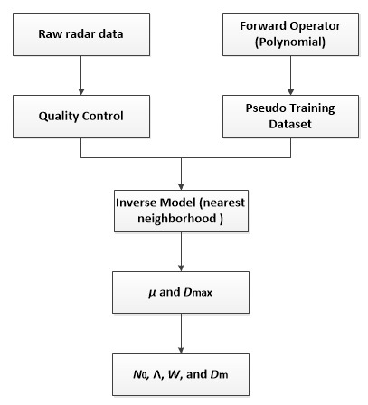
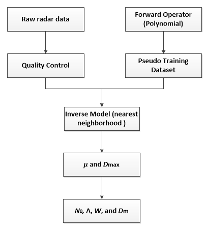
:This paper proposes an inverse model for raindrop size distribution (DSD) retrieval with polarimetric radar variables. In this method, a forward operator is first developed based on the simulations of monodisperse raindrops using a T-matrix method, and then approximated with a polynomial function to generate a pseudo training dataset by considering the maximum drop diameter in a truncated Gamma model for DSD. With the pseudo training data, a nearest-neighborhood method is optimized in terms of mass-weighted diameter and liquid water content. Finally, the inverse model is evaluated with simulated and real radar data, both of which yield better agreement with disdrometer observations compared to the existing Bayesian approach. In addition, the rainfall rate derived from the DSD by the inverse model is also improved when compared to the methods using the power-law relations.
1. Introduction
The raindrop size distribution (DSD) is one of the most important characteristics of a precipitating process, since the raindrop formation and its size evolution are related to the mechanism of cloud microphysics, kinetics, and thermodynamics. Weather radar is suited to obtain backscattering properties of the raindrops on mesoscale and convective scales when the raindrops form and descend toward the surface. The correct retrieval of DSD by radar is valuable for documenting and understanding the microphysical properties of a cloud system, increasing the accuracy of quantitative precipitation estimation, and improving the parameterization of numerical weather prediction. Potential applications include the flash flood warning, water resource management, reservoir construction, aviation, and weather modification.
The polarimetric weather radar has a long and profound impact on the remote sensing of atmosphere. Seliga and Bringi (1976) [1] first indicated that the ratio of the radar reflectivity at the horizontal and vertical polarizations, i.e., differential reflectivity, provided an additional evidence of distorted raindrops. Later, they [2] showed that the polarimetric measurements are in good agreement with model calculations of raindrops with a T-matrix method at S-band frequency. This technology was also transferred to attenuating frequencies, such as C-band [3] and X-band [4]. As the polarimetric radar transmits and receives the electromagnetic waves at two orthogonal polarizations, it also measures polarimetric variables, including differential reflectivity, differential phase shift, specific differential phase, and cross-correlation coefficient, when compared to the conventional radar [5,6]. By combining with absolute reflectivity, these variables can be used to determine the parameters in the truncated Gamma DSD [7,8].
In the literature, the algorithms for the DSD retrieval can be divided into two categories: One is a physical method and the other is a statistical approach. The physical method explores the direct relationship between the DSD parameters and polarimetric measurements. For example, the constraint method [9,10,11] uses radar reflectivity and differential reflectivity to retrieve the Gamma distribution by assuming an empirical relation between the slope and shape parameters. Meanwhile, the beta method [12] derives the effective slope of the axis ratio with respect to the diameter to make a better use of specific differential phase. This method also utilizes a normalized Gamma distribution [13] instead of the nonnormalized one [7], yielding a more realistic DSD [14]. However, it is evident that the constraint method has better consistency with the disdrometer data when compared to the beta method, since the beta method is sensitive to the noise of specific differential phase [15,16]. To reduce the noise effects, a power-law relation was employed for light rain in the beta method [17,18]. Moreover, the relations between the DSD parameters and polarimetric variables can be derived by using a reflectivity-weighted mean diameter [19,20]. This algorithm also considers the Mie effects at X-band frequency, to correct the rain-path attenuation. In addition, Raupach and Berne [21] retrieved the third and sixth moments to obtain a double-moment model for normalized DSD.
In contrast, the statistical approach approximates the nonlinear relation between the Gamma parameters and polarimetric variables with a mathematical process. Vulpiani et al. [22] proposed a regularized neural network method to give a non-parametric mapping from the polarimetric variables to the DSD parameters. Cao et al. [23] developed a Bayesian regression model by assuming the samples of radar measurements are independent and approaching to a Gaussian function. The Bayesian framework consists of a priori and a probability density function. If the probability density function is transferred to a penalty function, a variational method [24,25] can be used to obtain the associated parameters via an optimization procedure.
This study proposes a statistical approach to estimating the parameters of a truncated Gamma model for DSD with the polarimetric radar variables, called an inverse model. This approach designs a forward operator to calculate the polarimetric variables for a given DSD by assuming the shape and orientation of raindrops, ambient temperature, and radar wavelength. Furthermore, it approximates the forward operator with a polynomial function to generate a pseudo training dataset, which is inversely used to obtain the relation between the DSD and polarimetric variables. Finally, it adopts a non-parametric estimator based on a nearest-neighborhood method to retrieve the parameters within the truncated Gamma model. By comparing to the existing algorithms, there are some advantages of the inverse model. First, it uses pseudo training data generated by a forward operator to retrieve the DSD parameters inversely. These pseudo data are adjustable according to the dynamic range of the DSD parameters. Secondly, it can obtain the maximum drop diameter to yield a realistic Gamma model for DSD, whereas the existing algorithms generally assume the maximum drop diameter as a deterministic value or infinity. Thirdly, the model is optimized with regard to the mass-weighted mean diameter and liquid water content, since they are important for the Gamma representation of the DSD.
The paper is organized as follows: Section 2 presents the mathematical representations of the DSD and the microphysical quantities calculated by the DSD. It also introduces the dataset used in this study. Section 3 gives the forward operator for polarimetric variables and its polynomial approximation, which is used to generate a pseudo training dataset. In Section 4, a non-parametric estimator based on a nearest-neighborhood method for the DSD retrieval is proposed and its error characteristics are described. In Section 5, the performance of the proposed approach is evaluated by comparing to the existing Bayesian approach, while the rainfall rate derived from the DSD is also examined against the power-law relations. Finally, Section 6 provides a summary and some further discussions on the proposed method.
2. Representation of Raindrop Size Distribution
The raindrop size distribution is defined as the number density of raindrops per unit size range and per unit volume [26]. It plays a key role in the microphysics and dynamics of raindrops while falling in the atmosphere. Some instruments (e.g., disdrometer) can provide direct measurements of DSD by detecting individual drops with optical light illumination [27,28], whereas the measurements of remote sensing methods (e.g., radar) are indirect. That means the number density at a particular size bin cannot be obtained directly from radar measurements compared to the disdrometer. In this case, a parametric function has to be selected and transferred to represent the DSD of interest. A variety of theoretical distributions could be used for the DSD representation, including Gamma distribution [7,13], log-normal distribution [29], and exponential distribution [30], among others (e.g., [31]). In the literature, the most commonly used one is Gamma distribution, which is described in the following section.
2.1. Gamma Model
The Gamma function [7] is widely used to model the DSD in the precipitating system. It is formulated as
where is the size spectrum in mm−1 m−3, N0 is an intercept parameter in m−3, is a shape parameter in unitless, and is a slope parameter in mm−1. This definition is convenient since the corresponding moment (Mn in mmn m−3) of this distribution yields an explicit function other than an implicit integral form:
It is worth noting that Equation (1) represents the spectrum with a drop size from zero to infinity, thus the DSD moment in Equation (2) becomes an infinite integral accordingly. However, in nature, the measurements are often conducted within a limited sampling volume and time, and the resulting DSD is truncated in a finite size range . For example, the two-dimensional video disdrometer (2DVD) can measure drops with a diameter between 0.1 and 8 mm [32]. To reduce the number of parameters in the DSD model, the lower limit is often set to be zero [7], whereas an exception is an unusual DSD associated with a size-sorting effect due to updrafts and wind shear [33]. The Gamma model is then changed to [7]
and the corresponding moment is calculated as [8]
where is a lower incomplete Gamma function.
In Equation (1), the unit of the intercept parameter N0 varies according to the shape parameter . To obtain an independent intercept term, a normalized Gamma function is introduced by scaling the DSD in terms of liquid water content and mass-weighted mean diameter [13,34]. It is formulated as
where Nw is the normalized intercept term in mm−1 m−3, Dm is the mass-weighted mean diameter in mm, and is a normalization factor defined in [5]. The new intercept term Nw can be written as
where is the density of liquid water, and W is the liquid water content. The new term Nw is equivalent to the intercept of an exponential distribution with an identical liquid water content [5]. In addition, the slope parameter is substituted by an approximation expression:
which assumes the maximum diameter Dmax is sufficiently larger than the mass-weighted mean diameter Dm (Dmax/Dm2.5 [7,35]). The corresponding DSD moments can then be expressed as
with
Another normalization method, called a double-moment generalized Gamma model [21,36,37], takes into account two random DSD moments:
with
Further, the general moment can be derived from the relationship among the DSD moments:
with
2.2. Bulk Properties of DSD
The liquid water content W is calculated by using the third moment of DSD:
where the water density is considered as 1 g cm−3. The median volume diameter, D0 in mm, is the upper limit of raindrop size that contributes to half of the total liquid water content [5]:
Meanwhile, the mass-weighted mean diameter (Dm) is defined as the ratio of the fourth and third moments:
In the still air, the rainfall rate is determined by the combined effects of drop fall velocity and DSD, which is expressed as
2.3. Dataset
This study analyzed the polarimetric radar measurements collected by the Next Generation Weather Radar (NEXRAD) system located near Oklahoma City (35.333°N, 97.278°W), United States. The KTLX radar is a dual-polarization radar at a frequency of around 2.8 GHz, with a resolution of 250 m in range by 0.5 degree in azimuth below 2.4 degree in elevation. The minimum and maximum elevation ranges from 0.1 to 19.5 degree. We primarily analyzed the first unblocked scan (typically 0.5 degree) in VCP 212 mode updated in 4–6 min. The radar simultaneously measures three base data, i.e., radar reflectivity factor (Zh in mm6 m−3), mean Doppler velocity, and spectrum width, as well as three polarimetric variables, namely, differential reflectivity (Zdr in unitless), differential phase ( in degree), and cross-correlation coefficient at zero lag. The radar dataset is organized and processed using an open-source software package called the Python ARM Radar Toolkit (Py-ART), which has been widely used in weather radar community [41,42]. Prior to performing the DSD retrieval, the data fields were smoothed by a moving window with five range gates to reduce the noise effect, and the ground clutters are removed with a quality control procedure [43,44,45]. Furthermore, the specific differential phase (Kdp in degree km−1), which is the range derivative of , was computed using an iterative linear regression process [46] and compared with NEXRAD level 3 products [47,48]. Finally, this study utilized three processed radar variables, Zh, Zdr, and Kdp, since they are more sensitive to the variability of the DSD when compared to the others [6].
To validate the DSD retrieval method, a second-generation low-profile 2DVD [27] was deployed in the Kessler Atmospheric and Ecological Field Station (KAEFS) in southwest Oklahoma (34.9846°N, 97.5234°W), about 44.7 km away from the KTLX radar. The radar beam at an elevation of 0.5 degree is about 886 m higher than the disdrometer. Strong wind and turbulence may significantly affect the disdrometer measurements of raindrops [49]. Therefore, the disdrometer data were corrected by a terminal velocity filter following the theoretical relation between the diameter and velocity as in [39]. In addition, the time periods with total drop number less than 10 or rainfall rate less than 0.1 mm h−1 were excluded. The processed disdrometer dataset contained 63,806 1-min drop spectra in 852 rain events collected between 0524 UTC 17 June 2006 and 1658 UTC 18 January 2017.
3. Forward Operator for Polarimetric Variables
The polarimetric variables are sensitive to ensemble properties, such as particle size, shape, and different hydrometeor phases [50,51]. For a volume of raindrops, these variables depend on not only the size spectrum, but also the scattering amplitudes, which are determined by the shape and orientation of raindrops, ambient temperature, and radar wavelength. In this section, we first introduce the polarimetric variables used in the DSD retrieval, and then utilize a forward operator to prescribe the scattering amplitude across the size bin. It is simplified with a polynomial approximation, yielding an explicit form for calculating each variable based on the Gamma DSD assumption. Finally, the forward operator is used to generate a pseudo training dataset to optimize a non-parametric estimator that is detailed in the next section.
3.1. Polarimetric Variables
This study used three polarimetric variables on a linear scale, namely, radar reflectivity at horizontal (Zh) and vertical (Zv) polarizations, as well as specific differential phase (Kdp). The radar reflectivity can be calculated via the radar cross-section, dielectric constant, and DSD in case of a linear polarization:
where is the radar wavelength in millimeter, |K|2 is the water dielectric constant factor in unitless, and is the backward scattering amplitude in mm, of a raindrop with an equivalent-volume diameter (D; hereafter diameter):
where a is the transverse semi-axis in mm and b is the symmetry semi-axis in mm.
Furthermore, the differential reflectivity (Zdr) is defined as the ratio of the radar reflectivity at the two polarizations:
The specific differential phase is mathematically formulated as the integral of the real part of the propagation constant difference and DSD:
where are the forward scattering amplitudes for particles with a diameter D at the horizontal and vertical polarizations, respectively, and represents the real part of the scattering amplitude.
In this paper, the scattering amplitudes are computed by using T-matrix codes for non-spherical particles [52,53]. The oblate raindrops with the symmetry semi-axis b less than the transverse semi-axis a are uniformly distributed in a volume with a known size spectrum. Moreover, axis ratio (b/a) is a key parameter for computations of reflectivity and phase shift at the two orthogonal polarizations. To characterize the relationship between the diameter and axis ratio in an analytic form, a universal equation is applied following the observational work in [38], with a modification that the drops with diameters less than 0.5 mm are spherical [26]. This relation is expressed as
The dielectric constant is obtained by calculating the complex indices of refraction following the least square fit of the Debye equations [54], with assumptions that the ambient temperature is 10 °C and the radar wavelength is 10.8 cm. It is noted that one typical temperature is selected for T-matrix simulations for raindrops, and the effects of temperature variation have been investigated in previous studies [5,20]. The canting angle distribution has been studied under experimental conditions [55,56]. In this study, we considered a Gaussian distribution with zero mean and small variance (10°).
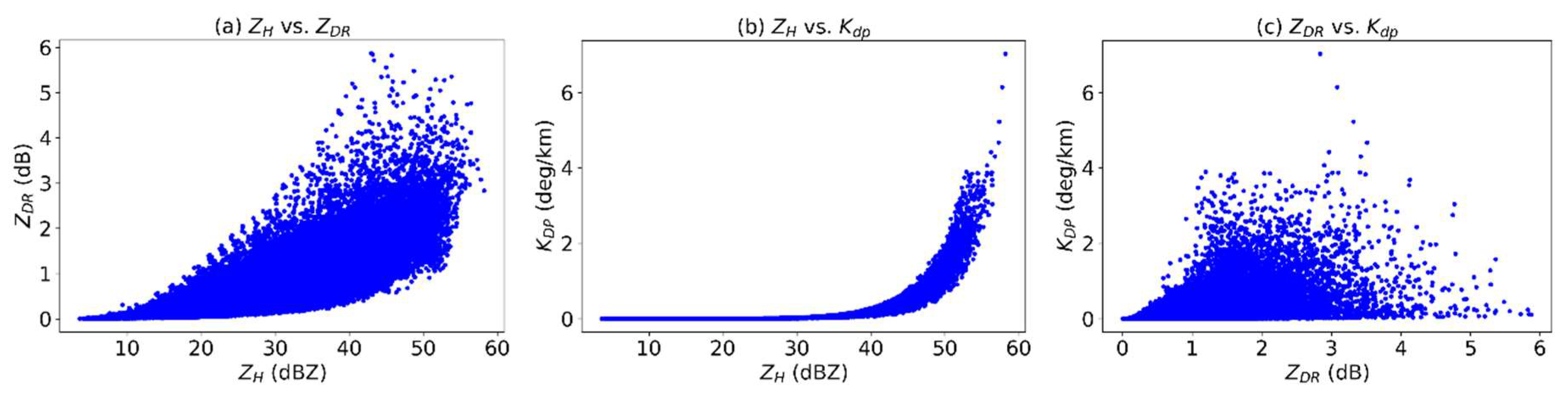
Figure 1 shows the characteristics of the three polarimetric variables simulated using the disdrometer observations. In Figure 1a, it is clear that Zdr is gradually rising with Zh going up. However, this increasing trend is negligible when Zh is below 0 dBZ, indicating these DSDs are dominated by small spheroid drops. The values of Zdr then have a rapid growth when Zh is over 0 dBZ, while the spreads of Zdr become wider. This might show that the corresponding DSDs contain a significant amount of oblate median-size and large drops. Similarly, Figure 1b illustrates that the values of Kdp remain relatively stable at 0 deg km−1 for Zh below 37 dBZ, following a boom in Kdp when Zh is larger than 37 dBZ. When Kdp is very small, it is difficult to accurately estimate the DSD parameters due to the noise effect [12], thus a self-consistency method may be used to provide an additional constraint for the data with Zh below 37 dBZ [57]. For the scatterplot of Zdr and Kdp (Figure 1c), it is interesting to note that, when Zdr reaches 5 dB, Kdp could stay below 0.5 deg km−1, implying the forward scattering amplitude may significantly differ from the backward one due to Mie scattering.
Table 1 shows the means, standard deviations, minima, and maxima of microphysical quantities and polarimetric variables simulated using the disdrometer data. It is noticeable that the means of microphysical quantities (Dm, W, and R) are generally small, since the entire dataset is dominated by light rain and drizzle. However, as the moderate and heavy rain cases are taken into account, the probability distributions of these quantities are significantly widened, producing relatively large standard deviations. Furthermore, the dynamic range of Zh on a linear scale reaches mm6 m−3 corresponding to 479.5 mm h−1 for R, whereas the ones for Zdr and Kdp on a linear scale are 3.86 and 7.03 deg km−1, respectively, which are much smaller than that of Zh and R. This implies that small measurement errors of Zdr and Kdp may result in a significant bias on R comparing to Zh. In contrast, the dynamic ranges of Zdr and Kdp are comparable to that of Dm and W, indicating a good estimation can be achieved using these variables.
3.2. Forward Operator
In Equation (19), it can be found that the scattering amplitude is independent from the DSD at each size bin. If the scattering amplitude is considered a forward operator, Equation (19) can be transferred as
where is the scattering amplitudes at the horizontal and vertical polarizations, respectively, is the integration operator, and is thus the forward operators for the radar reflectivity. Similarly, Kdp is computed in terms of a forward operator:
where is the amplitude of the forward operator of Kdp.
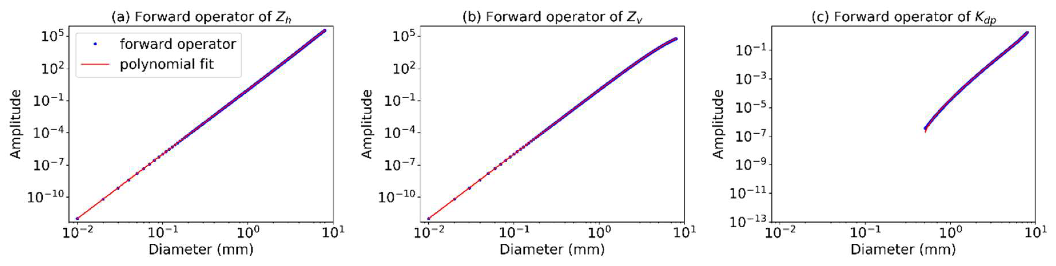
The forward operators of Zh, Zv, and Kdp can be obtained by performing simulations of monodisperse raindrops with diameters varying from 0.01 mm to 8 mm. As shown in Figure 2a, the forward operator presents a quasi-linear shape in a logarithmic coordinate, while the amplitude of the forward operator monotonically increases with the diameter climbing up. This quasi-linear shape on a logarithmic scale suggests a polynomial relationship between the diameter and the amplitude on a linear scale, which is consistent with the Rayleigh approximation. Similarly, Figure 2b also illustrates a progressively increasing trend for the forward operator of Zv. A noticeable difference can be seen when the diameter is larger than 1 mm, where the vertical amplitude of a larger drop grows relatively slower than the horizontal dimension. On the one hand, it is because the contribution of the vertical dimension (b axis) to the diameter D in Equation (20) significantly differs from that of the horizontal dimension (a axis). On the other hand, as the diameter gets larger, the axis ratio in Equation (23) gives a large discrepancy from the unity, which indicates that the large raindrops tend to be more oblate than small drops. Under the Rayleigh assumption, the radar cross section at a particular polarization is proportional to sixth order of the corresponding geometric dimension of a raindrop. Therefore, the amplitude at the vertical polarization is generally smaller than that at the horizontal polarization, particularly for larger raindrops. Moreover, Figure 2c shows that the forward operator of Kdp is also characterized by a monotonically increasing curve, but the amplitude of forward operator is equal to zero when the diameter is less than 0.5 mm, due to unity axis ratio at this diameter range in Equation (23). In addition, in this region, the forward operators of Zh and Zv are identical, yielding Zdr equal to 1 (0 dB).
Figure 2 shows that the amplitudes of the forward operators for Zh, Zv, and Kdp may have a quasi-linear relation as a function of the diameter on a logarithmic scale, which is equivalent to a polynomial on a linear scale. Therefore, the forward operator may be approximated by a polynomial function to avoid the implicit integral form in Equations (19) and (22), by using the Gamma model of the DSD. Since the amplitude is several orders higher than the diameter, a basis polynomial needs to be selected, and then the residuals are fitted into a high-order polynomial expansion. It can be formulated as
where b is the order number for the basis polynomial, p is the maximum order number for the polynomial fit, and ai is the polynomial coefficient for the order i.
To obtain the optimal performance for the fitting, the mean square error (MSE) is used to select the polynomial model. It is defined as
where p is predicted values and a are actual values.
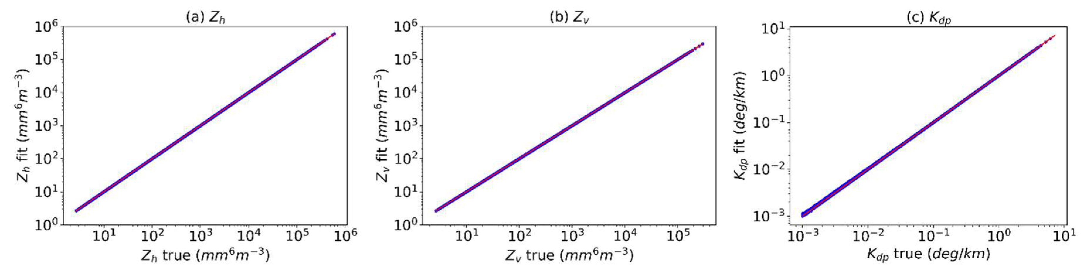
Figure 3a illustrates that the MSE of Zh is generally reduced as the basis order increases from 3 to 6, whereas the basis order of 7 produces a significant error by comparing to the others. Therefore, the basis order for Zh is set as 6 based on the MSE test. Furthermore, for the curve with the basis order of 6, the MSE gradually decreases as the order p goes down, while a sharp fall can be found between 2 and 3. When p is larger than 3, the decline trend becomes steady. Consequently, we set p as 3 to achieve a balance between the model complexity and approximation accuracy. The fitting results are in good agreement with T-matrix computations, as shown in Figure 2a. Moreover, when the polynomial fit is applied to the real DSD, it agrees well with disdrometer data in Figure 4a, with small bias, relative error, and MSE as well as high correlation coefficient (CC) in Table 2.
As shown in Figure 3b, the basis orders of 4 and 5 for Zv can yield even better MSEs than that of 6 when p is relatively large (6–9). However, the higher accuracy of fitting results from overfitting of the data samples by the model with high complexity, which is evident from the comparison between the data and fitting curve of higher orders (not shown). Following a way similar to Zh, the b and p for Zv are set as 6 and 4, respectively, yielding a good consistency in terms of bias, relative error, MSE, and CC (Table 2), when applied to the monodisperse raindrops (Figure 2b) and real DSDs (Figure 4b).
The selection of order number of polynomial model for Kdp is more straightforward than Zh and Zv (Figure 3c). The curve with the basis order of 4 generally gives the lowest MSE among the ones from 3 to 7. Meanwhile, the polynomial order is set to as 4, since the MSEs of p larger than 4 become stable at around . Note the fitting range for Kdp is from 0.5 to 8 mm rather than from 0.01 to 8 mm for Zh and Zv. Figure 2c shows the comparison between the data and the fitting results, where a relatively large difference can be found for the diameter between 0.5 and 0.7 mm. When the real DSDs are considered, an increase of uncertainty is expected for Kdp below 0.01 deg km−1 (Figure 4c). The rest of the coefficients in Equation (26) are listed in Table 2.
3.3. Pseudo Training Dataset
On substituting Equation (26) into Equations (24) and (25), and assuming the Gamma model for the DSD, the polarimetric variables can be re-written as
and
where Mi+b is the (i + b)th DSD moments obtained by multiplying N(D) in Equations (24) and (25) with Di+b in Equation (26). To eliminate the factor N0, the ratios between Zh and Zv, and between Zh and Kdp are taken into consideration, yielding
and
where x1 and x2 are the training data; the subscripts h, v, and d represent the parameter set of b, p, and ai for Zh, Zv, and Kdp, respectively; the minimum diameter for calculation of Kdp is 0.5 mm; and , , and Dmax are the parameters in the Gamma model retrieved by x1 and x2. Since three dependent variables need to be estimated by two independent variables, the solution of the DSD retrieval may be unstable, thus an empirical constraining assumption has to be made, e.g., the - relation used in [11]. Although this relation is believed to be valid for limited types of rain events [58] and subjective to the minimum diameter and data filtering [59], it arises from the actual rain microphysical processes [60,61]. An alternative approach to the two-parameter solution is based on the joint probability distribution of the parameters within the raindrop mass spectrum [62].
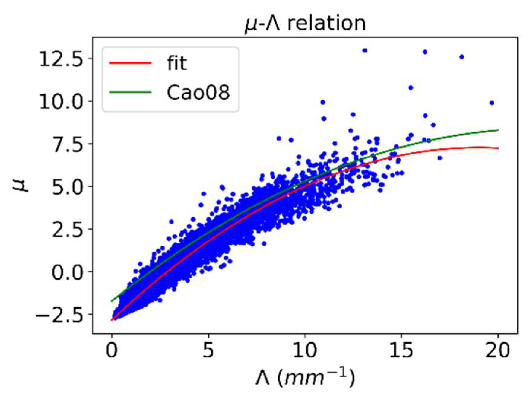
In this study, we use the thresholds of rainfall rate larger than 5 mm h−1 and total number counts larger than 1000 drops min−1 to avoid the fluctuations arisen from DSD fitting, which is consistent with the studies in [11,63]. It yields the relation as
Figure 5 illustrates the curve for the - relation obtained by using the ten-year disdrometer data. The result is generally consistent with the previous study in [63]. However, the MSE is 0.184 for our relation, whereas it is 0.727 for the relation in [63].
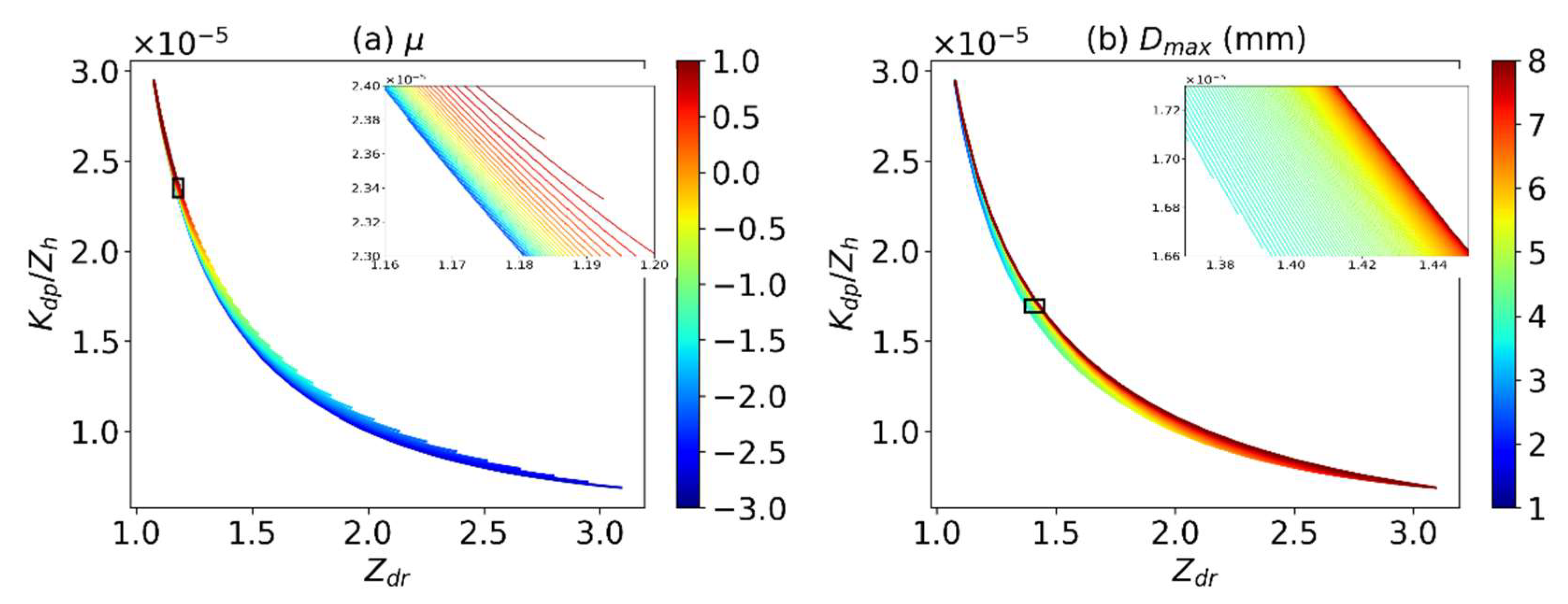
Finally, the training dataset, Zdr and Kdp/Zh, can be generated via Equations (30)–(32), by drawing and Dmax. Based on the observations of dynamic ranges of and Dmax in the ten-year-disdrometer data, we assume that the drawing poll ranges from −3 to 20 for and from 1.7 mm to 8 mm for Dmax, with an additional constraint that Dm is no larger than Dmax. Figure 6 presents the simulation results of the training dataset Zdr and Kdp/Zh projected onto a two-dimensional plane by assuming a number of fixed and Dmax, respectively. In Figure 6a,b, Kdp/Zh dramatically drops with Zdr increasing when Zdr less than 2. The decreasing trend then becomes steady, showing a concave curve. Furthermore, for identical Zdr, the values of Kdp/Zh rise as or Dmax climbs up, while for identical Kdp/Zh, the values of Zdr also increase with or Dmax going up. In addition, when Zdr is relatively small (less than 0.318 dB), the colored curves in Figure 6 may not be disjoint. It means that two distinct parameter sets of and Dmax can generate identical training data of Zdr and Kdp/Zh, leading to instability of an inverse model. To tackle this problem, we separate the data with instability by applying a threshold of Zdr less than 0.318 dB. As shown in Figure 6, by applying this threshold, the training dataset is well-separated and the corresponding curves are mutually disjoint. As a result, the problem of inversion of polarimetric variables to Gamma parameters is stable, and the retrieval uncertainty directly relates to measurement errors exclusively.
4. Inverse Model for Gamma Parameter Retrieval
The previous section shows that the polarimetric variables are calculated by the DSDs via the forward operator. Since the generated data are uniquely associated with the physical parameters, the data may be used to retrieve the DSD parameters inversely. In this section, we first introduce a non-parametric model to solve the inverse problem, and then select the optimal model by using real DSD data. Finally, we show the effect of the measurement error on the DSD retrieval.
4.1. Non-Parametric Estimator for the Inverse Model
There are some approaches to solving the inverse problem if the training dataset is available, such as Neural Network [64], Bayesian method [65], and variational method [66]. In this paper, we adopt a nearest neighborhood method, due to its nature of simplicity and high speed.
The idea of the nearest neighborhood method is to use the observations in the training set closest in the feature space (i.e., a space composed by the polarimetric variables) to the input x to estimate the output y. Let and ; the k-nearest neighbor estimate is then defined as
where Nk(x) is the neighborhood defined by the kth closest points to x in the training dataset, and the metric of closeness is the Euclidean distance. Since the two independent variables have very different dynamic ranges, it is necessary to perform the normalization of the variables, which produces a zero-mean and unity covariance matrix. The procedures based on Cholesky factorization [50,67] is described as:
- Subtract the averaged values from the data matrix.
- Calculate the covariance of the residual matrix.
- Calculate an upper-triangular matrix of the covariance using Cholesky factorization.
- Divisde the residual matrix by the upper-triangular matrix.
Afterwards, the k observations closest to x in the feature space are averaged to give the retrievals of and Dmax. Finally, we calculate the estimates of the intercept N0 by substituting the and Dmax estimates into Equations (28) and (29) and take an average of the estimates to obtain the N0.
4.2. Model Selection
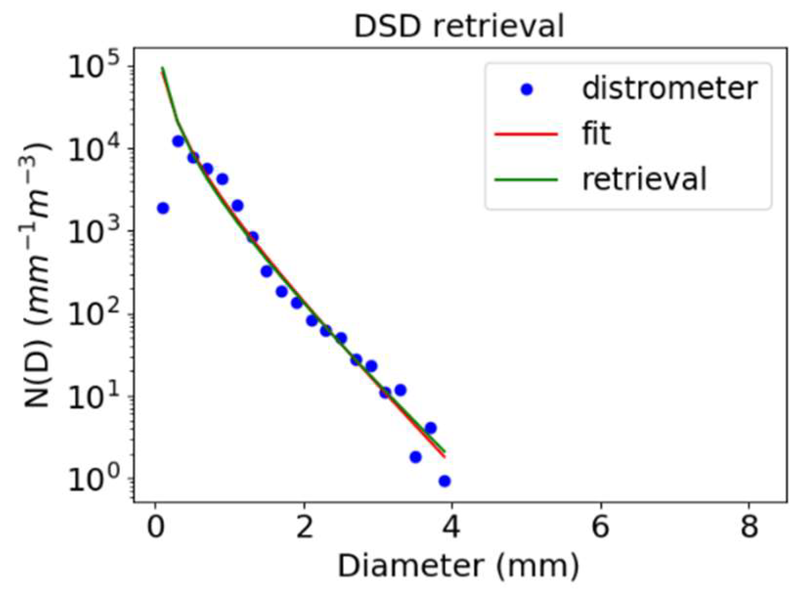
The performance of the nearest-neighborhood estimator relates to its capability of prediction on an independent test set of the real data. It is fundamentally important to assess this performance, since it determines the selection of the model, and provides a metric of the model quality. The statistical methods commonly search for the minimum of the MSE of in Equation (33), yielding an optimal model for estimation of the target variables y. However, as shown in Figure 7, the DSD observed by disdrometer may suffer from significant model errors with the assumption of the Gamma shape. At some stages of a precipitating process, the DSD occasionally exhibits a bi-modal or tri-modal distribution [68,69,70]. In addition, some errors may also arise from the moment method used to fit the Gamma function to the disdrometer observations [60,71]. Due to these problems, the polarimetric variables may result in a retrieval of Gamma parameters that is significantly different from the true DSD (Figure 7).
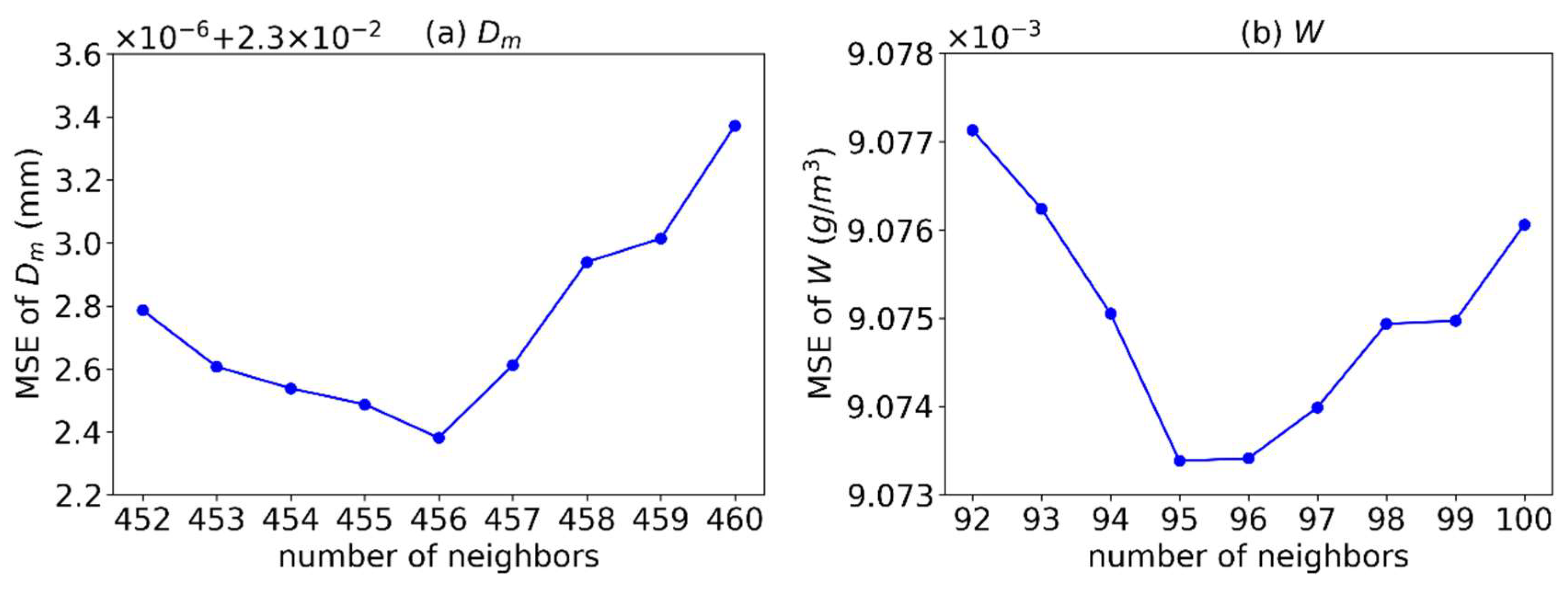
It is noticeable that the liquid water content (W) and mass-weighted mean diameter (Dm) in Equations (5) and (6) play an important role in the representation of the DSD. Furthermore, the deviation of a Gamma function from the disdrometer observations depends on these two microphysical quantities [17,18,72]. Therefore, the objective functions of the inverse model may be modified to produce a DSD retrieval similar to the disdrometer-derived Gamma parameters. To obtain a number for k neighbors, we search that yields an optimal estimate of Dm by using Equation (32). Furthermore, we determine the k neighbors of Dmax by optimizing W via Equation (14), where N0 is computed using Equations (28) and (29). Figure 8 illustrates the MSEs of W and Dm associated with the model complexity. The optimal numbers are 456 for and 96 for Dmax, but they are also affected by the spacing of data points in the pseudo training dataset.
4.3. Error Characteristics
Practically, it is difficult to obtain the polarimetric radar data free of measurement errors. These errors may have a significant impact on DSD retrievals, and sometimes lead to meaningless results. Therefore, it is important to evaluate the magnitude of the errors.
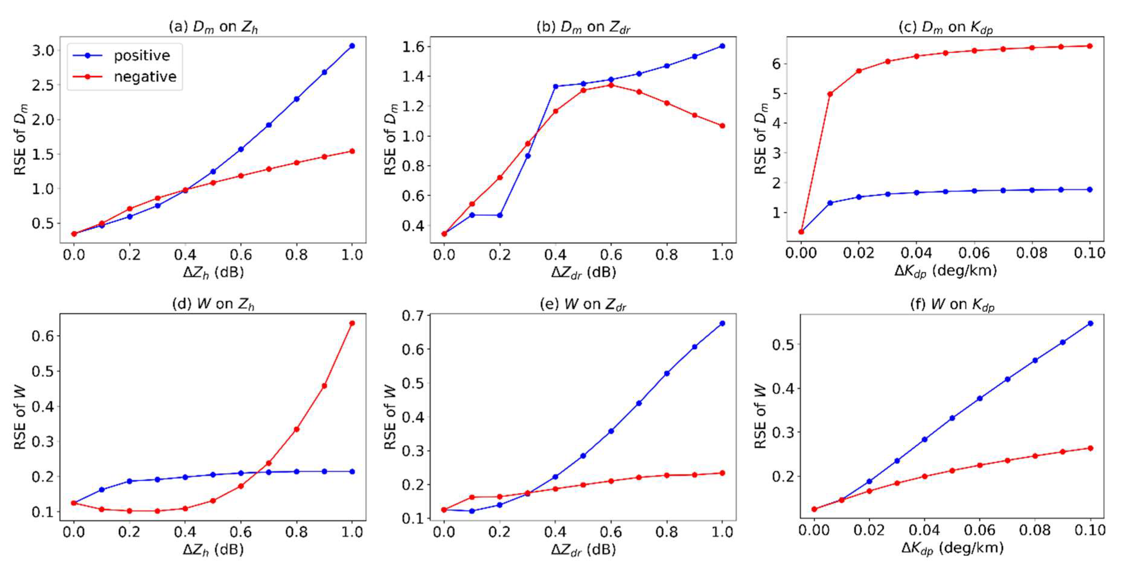
The problem may be formulated as follows. With the assumption of the perfect accuracy of the measurements of Zdr and Kdp, the uncertainties of Dm and W would correspond to that in Zh exclusively. Since the radar records Zh measurements on a logarithmic scale, the impacts of the relative error (ΔZh) in decibel are assessed. This analysis can also be applied to Zdr and Kdp, but Kdp needs to be considered on a linear scale. Note that we study the characteristics of relative square error (RSE), which is defined as
where
Figure 9 illustrates the analysis of error characteristics on Zh, Zdr, and Kdp, respectively, in the disdrometer dataset. In Figure 9a, the RSE of Dm generally presents an increasing trend associated with either the positive or negative ΔZh. In practice, for ΔZh < 0.3 dB, the RSE for positive ΔZh is not very large (less than 1), and it becomes large beyond this limit. By contrast, the RSE for negative ΔZh rises slowly, but it is more sensitive to ΔZh between 0.1 and 0.4 dB, leading to a lower threshold of 0.2 dB for the RSE less than 1. Moreover, the RSE of W for positive ΔZh increases rapidly when ΔZh < 0.2 dB and remains steady at around 0.2 (Figure 9d). It is interesting to note that the RSE of W for negative ΔZh decreases slightly when ΔZh is below 0.2 dB. This is because Equations (28) and (29) may produce distinct estimates of N0, where Zh often gives the largest one. By adding a negative error, the variance of N0 estimates is reduced, yielding a slightly improved W.
The dependence of the uncertainty of Dm and W on Zdr errors (Figure 9b,e) generally preserves the trend similar to the previous case (Figure 9a,d), however, some distinct features are noticeable. In Figure 9b, the RSE of Dm for positive ΔZdr shows a dramatic rise between 0.2 dB and 0.4 dB. It may indicate a threshold of 0.2 dB for Zdr to obtain an accurate estimate of Dm, while the RSE is below 0.6 for negative ΔZdr less than 0.1 dB. Furthermore, Figure 9e presents a local minimum for ΔZdr at around 0.1 dB. Apart from the reduction of the variance of N0 estimates, this minimum may be due to an effect of the thresholding of Zdr prior to performing the nearest-neighborhood estimator. With the positive ΔZdr adding to the data, the number of points for the calculation of RSE increases more significantly than the squared errors, resulting in a slight decrease of RSE. Moreover, it is clear that Dm is very sensitive to Kdp errors, since a small value (e.g., 0.01 deg km−1) can lead to a boom in RSE, particularly for negative bias (Figure 9c). To determine a threshold for Kdp error, it can be found that the growth rate of RSE for positive ΔKdp is accelerated when Kdp is larger than about 0.01 deg km−1 (Figure 9f), while the RSEs of the two types of errors are both small (below 0.2).
The important conclusion of this analysis is that, if the Dm and W are retrieved by using the polarimetric variables, we suggest the thresholds of 0.2 dB, 0.1 dB, and 0.01 deg km−1 be applied to the errors of Zh, Zdr, and Kdp, respectively.
5. Results
In this section, the inverse model (IM) for the DSD retrieval is first tested with polarimetric data simulated by the ten-year disdrometer observations, and compared to an existing algorithm designed for the same regime [23], called a Bayesian approach (BA). Furthermore, the model is applied to the five-year joint observations of dual-polarized radar and disdrometer to assess its performance on real radar data. Finally, the rainfall rate calculated by the DSD is compared to the results of the power-law relations to evaluate the potential of an operational application. In addition to mean square error (MSE) and relative square error (RSE), we also use mean absolute error (MAE),
relative absolute error (RAE),
correlation coefficient (CC),
where
root mean square error (RMSE),
and root relative square error (RRSE),
5.1. DSD Retrieval with Disdrometer-Simulated Data
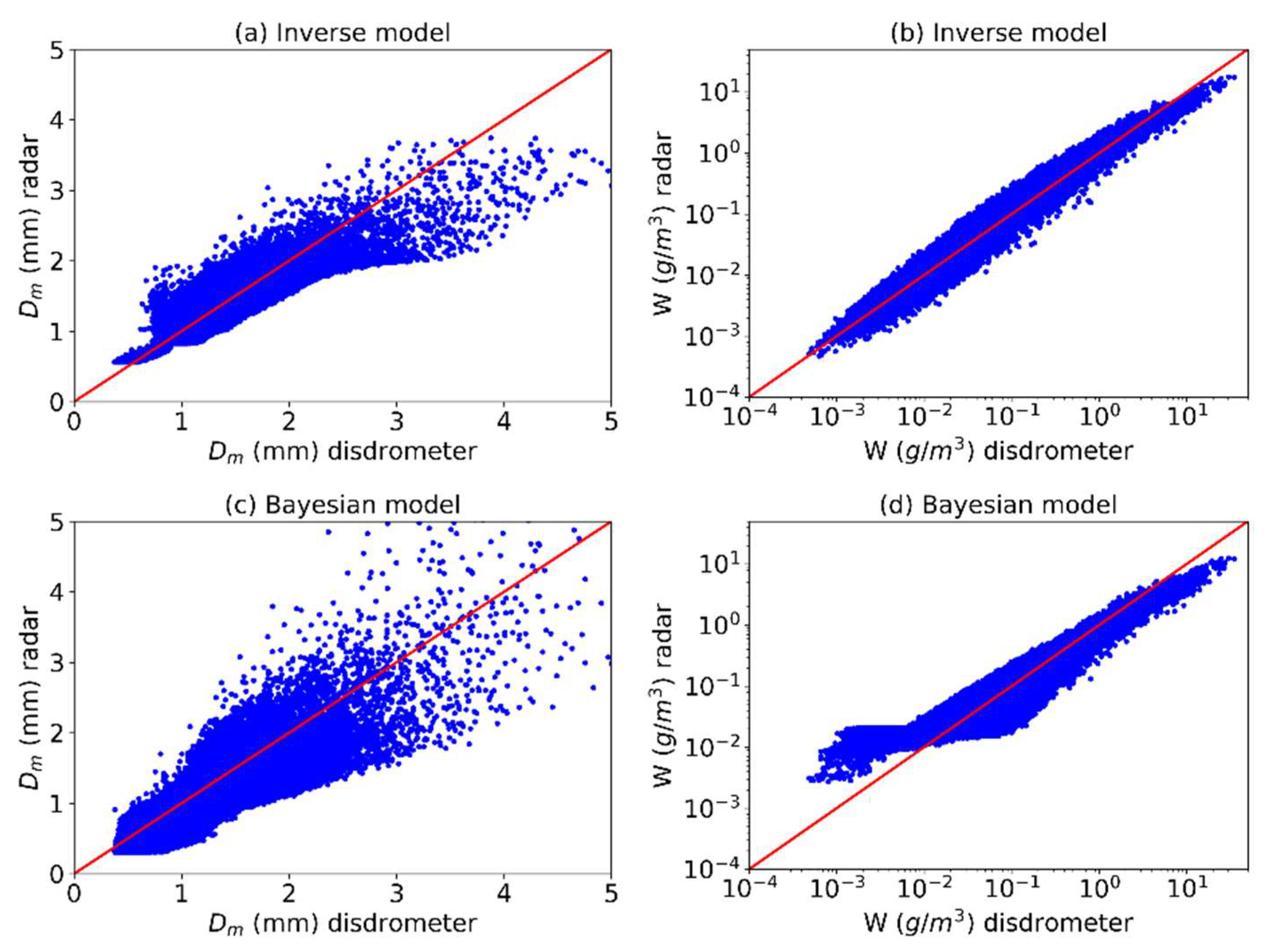
At the first stage of the assessment, we apply IM to the simulated dataset (see Section 3.1) and compare to BA. Figure 10 illustrates the comparison between the disdrometer observations and the DSD retrievals. As shown in Figure 10a, the Dm results from IM show good consistency with the disdrometer data for Dm less than 0.8 mm, while a boundary exists at around 0.8 mm due to the Zdr threshold of 0.318 dB. When Dm is between 0.8 mm and 2.5 mm, the retrievals fairly agree with the disdrometer data, following a large spread for Dm larger than 2.5 mm. By contrast, the uncertainty of the retrievals by BA gradually increases as Dm goes up, particularly for Dm larger than 2 mm (Figure 10b). Since the Bayesian approach constructs the joint distribution of polarimetric variables and DSD parameters from the radar data, it gives a better performance on the lower end comparing to IM. By analyzing the statistics in Table 3, it is clear that the Dm retrievals by IM outperform that by BA. The MSE and RSE of IM are generally one third of BA, while the MAE and RAE of IM are half than of BA. The difference of the CC is less pronounced, with IM at 0.917 and BA at 0.821.
Figure 10b,d shows the comparison of W obtained by IM and BA, respectively. The retrievals of W by IM well match the disdrometer observations between 0.001 g m−3 and 10 g m−3. When W is above 10 g m−3, the points tend to be below the red curve, indicating an underestimation of W at this range. By comparing to IM, BA gives higher estimates when W below 0.01 g m−3, while it underestimates W above 5 g m−3 (Figure 10d). In addition, it shows high density at around 0.01 g m−3 in BA, due to small priori below 0.01 g m−3 [23]. As shown in Table 3, the statistics of IM are generally improved in terms of MSE, MAE, RSE, RAE, and CC. Notably, the retrievals of W by IM and BA both achieve a high CC, yielding good agreement between retrievals and observations.
It can be found that Zh and Zv are generally proportional to the sixth-order moment of DSD, while the basis polynomial of Kdp is on the fourth order (Section 3). For the simulation data, IM yields high accuracy for the sixth-order moment, Z, with RSE of 2.4 and CC of 0.9989, but very low accuracy for the zero-order moment (or total number concentration), Nt, with RSE of 3.2 and CC of 0.6183. In contrast, the zeroth and sixth moments estimated by BA are less accurate, while RSE for Nt and Z are 77.5 and 0.050, and CC are 0.2417 and 0.6884, respectively.
5.2. DSD Retrieval with Real Radar Data
When the inverse model is applied to real radar data, some problems may arise due to the sampling difference between the instruments. The radar beam often illuminates the hydrometeors at a higher altitude due to the curvature of the earth surface and the radar elevation angle. In our study, we used the first unblocked radar elevation (approximately at 0.5°), thus the altitude difference between the two instruments is about 886 m by considering the altitude of radar location. During the falling of raindrops, their size distribution may evolve as a result of coalescence, collision, breakup, accretion of droplets, and evaporation. Moreover, the polarimetric variables are calculated from the disdrometer observations under the assumption that the raindrops uniformly distributed in the radar volume. However, the radar resolution volume above the disdrometer location is about 3.91 m3, whereas the sensing volume of the disdrometer is around 2.4 m3. Therefore, the variables may be biased in the real case if the radar volume is not filled completely. These sampling problems lead to an uncertainty when real radar data are used for the DSD retrieval.
To compare the radar measurements with the disdrometer observations, a Cartesian coordinate was established with the origin located at the radar center. The perpendicular coordinate of the disdrometer relative to the radar center was then calculated with the haversine formula [73]. To achieve a good consistency, we selected five radar gates closest to the disdrometer coordinate and shift the disdrometer data within min for each precipitating process, corresponding to the radar temporal resolution of 4–6 min. The pairs of the radar data and disdrometer data with the highest correlation were processed as a validation dataset for the DSD retrieval. In addition, the mean bias was deduced from the radar measurements for each rain process.
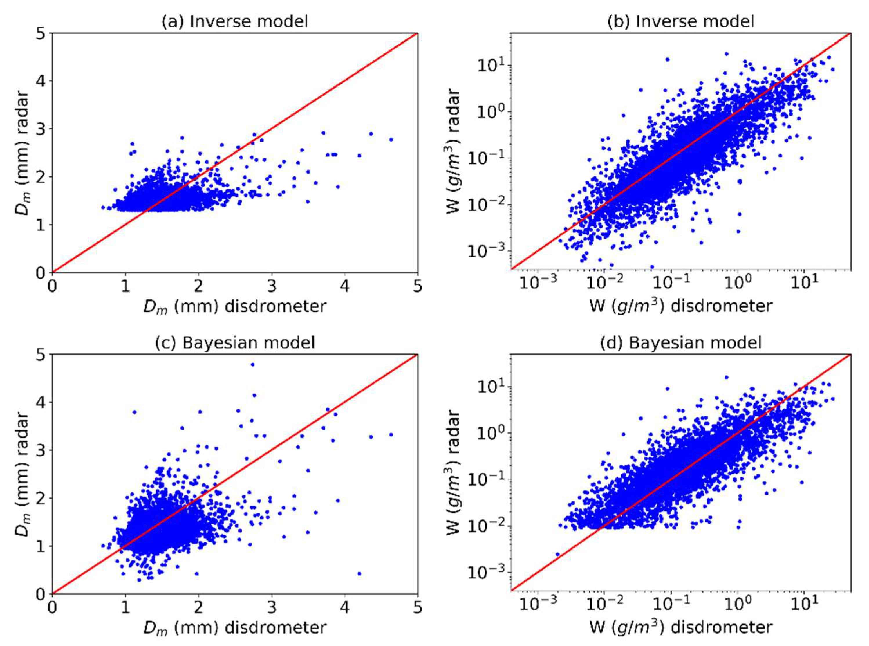
Figure 11 illustrates the comparison between Dm and W obtained by IM and BA using real radar data. It is noticeable that the Dm retrievals by IM concentrate on the range between 1.2 and 2.8 mm, whereas there is a large variation for the retrievals by BA. The BA retrievals also show a lower bound at around 0.01 g m−3; by contrast, the IM ones are less biased in this region. Furthermore, the statistics in Table 4 indicate that IM achieves better agreement than BA in terms of MSE, MAE, RSE, and RAE, but CCs for the two models are generally low. In addition, the W retrievals by IM and BA have a wide spread when compared to the results of the simulated data, due to the measurement errors, noise, and sampling problems.
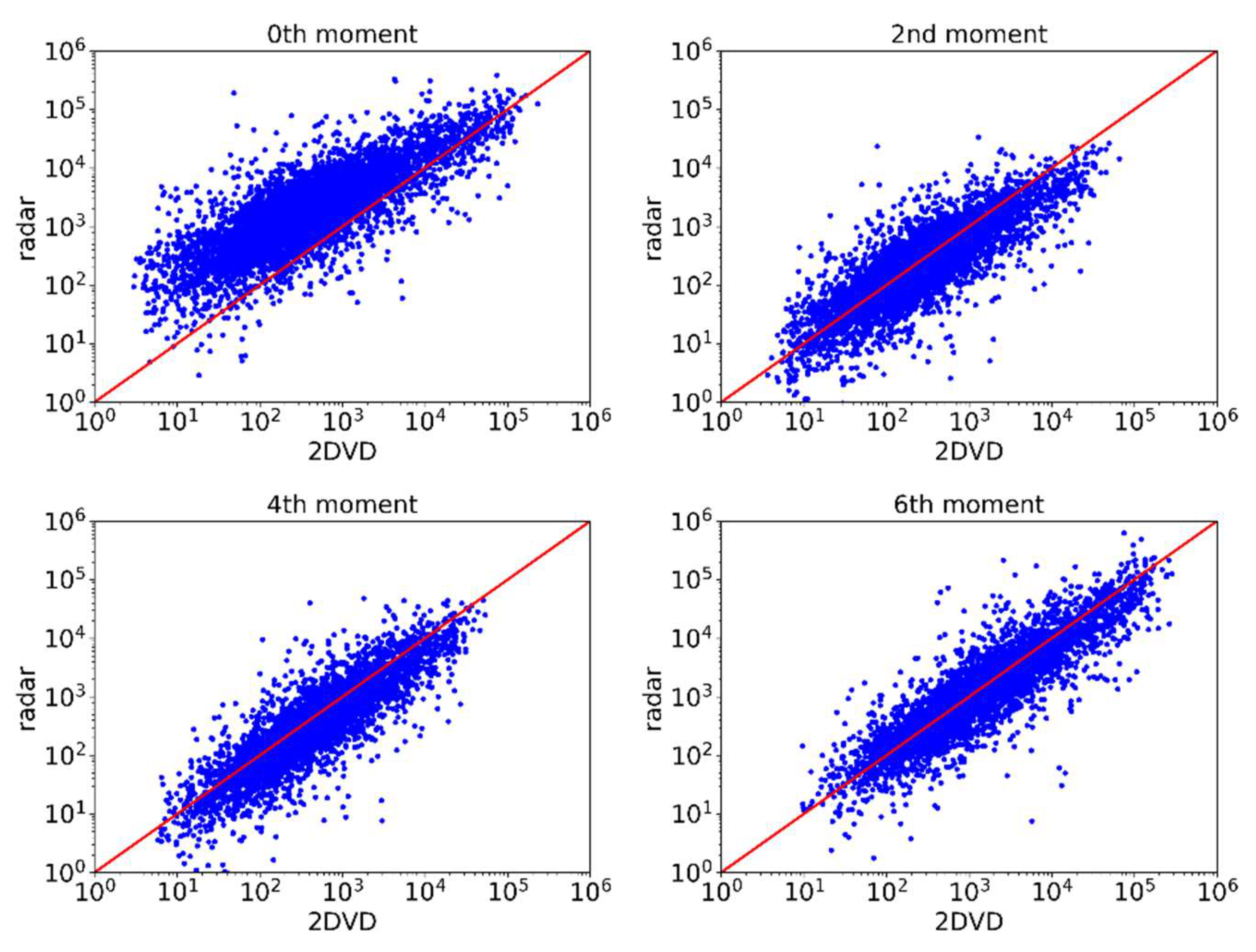
It is also very important to evaluate the DSD moments obtained by the inverse model, since the moments play an important role in the representation of the DSD. In this study, we compared the zeroth, second, fourth, and sixth moments, which are commonly used in the DSD estimation [21,37,74]. Since the infinite zeroth-moment sometimes results from less than −1, an approximation method has been used. We first calculated the drop concentration N(D) at each size bin using Equation (3), and then integrated the moment concentration . By using this approximation method, the zeroth-moment can yield valid error statistics, while the second, fourth, and sixth moments remain the values calculated by Equation (4). In addition, the Bayesian method has constructed the prior probability with W and Dm, leading to invalid by solving the quadratic equation in Equation (7). Therefore, the DSD moments calculated by the Bayesian retrievals are not presented here.
Figure 12 illustrates the comparison of the moments calculated by the disdrometer observations and retrieved by the radar data. The red curve (reference) crosses the region of high intensity of the blue dots (data) for the second, fourth, and sixth moments. However, the blue dots for the zeroth moment tend to be biased toward the ordinate, leading to an overestimation.
The statistics in Table 5 provide quantitative assessment for the performance on the moment estimation. In general, for RMSE, MAE, RRSE, and CC, the second and fourth moments yield better results when compared to the zero and sixth moments, since the inverse model is optimized by W, which is proportional to the third-order moment. By contrast, RAE is constantly reducing as the order increases. In addition, the RMSEs and MAEs of the zeroth and sixth moment are much larger than the others, due to the significance of its magnitude.
5.3. Rainfall Rate Estimation
The rainfall rate estimation is one of the most important applications of polarimetric weather radar [75]. Since the rainfall rate in Equation (18) is related to DSD, a physical relationship between the polarimetric variables and rainfall rate exists. For rainfalls at the experiment site, the curves of Zh and R in a logarithmic scale present a linear shape, and therefore, yield an empirical relation as
By applying Zdr to the Z-R relation, the performance of the rainfall rate estimation is improved, as demonstrated in the JPOLE field experiment [76]. The dual-polarization algorithm is expressed as
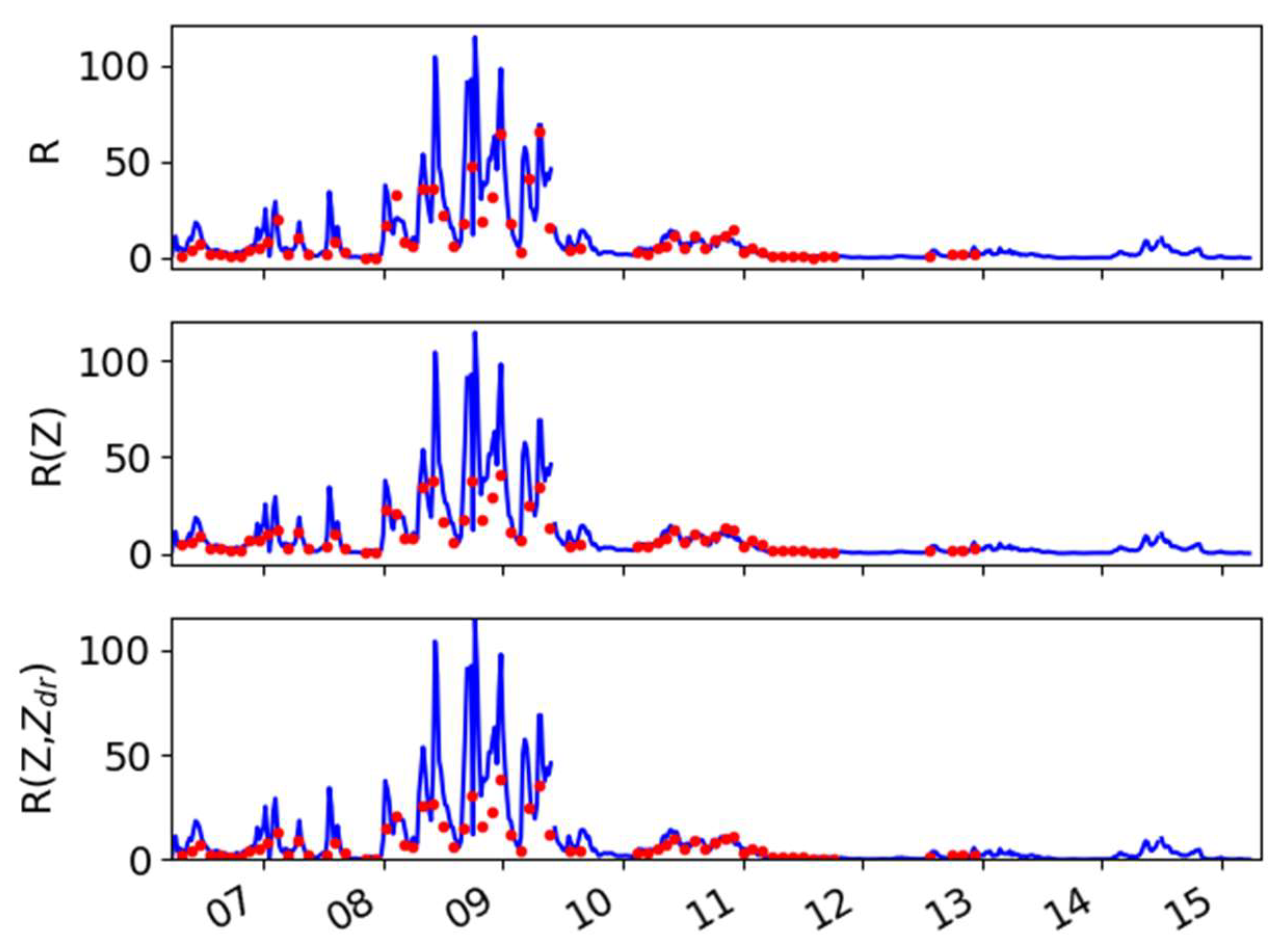
In this study, we compared the rainfall rate of the inverse model (IM) calculated by Equation (18) with that of the existing algorithms R(Zh) in Equation (44) and R(Zh, Zdr) in Equation (45).
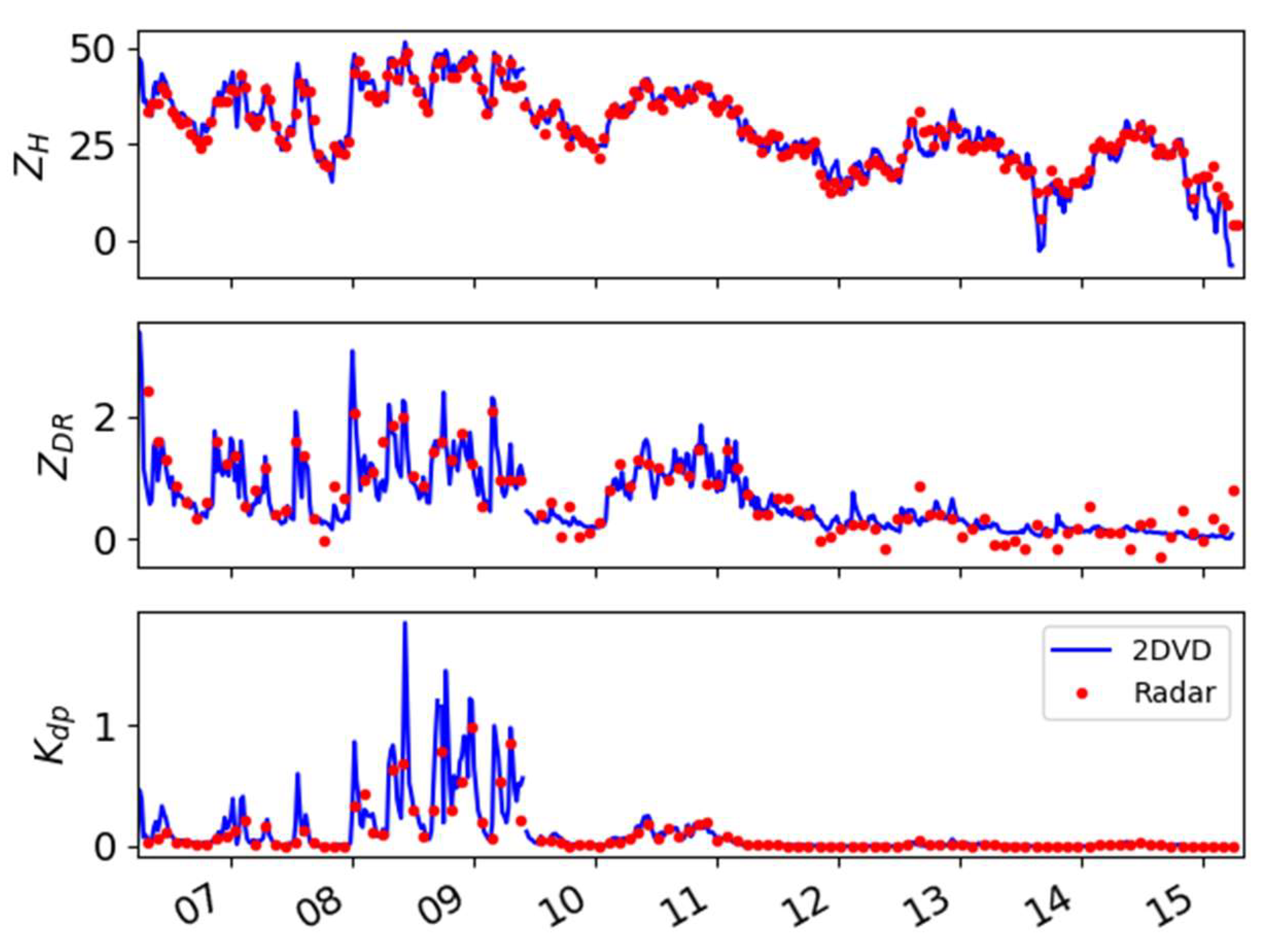
Figure 13 illustrates the time series of the radar measurements of a convective case that occurred between 0614 and 1519 UTC on 8 June 2014. The precipitating system arrived at the location of the disdrometer at the mature stage, with a maximum reflectivity of 51.5 dBZ. As it propagated eastward, the system gradually decayed and reached an average of 25 dBZ between 1200 and 1500 UTC. Furthermore, there was a large variation in the time series of the polarimetric variables Zdr and Kdp between 0800 and 0930 UTC, associated with the DSD variability during the mature stage. The two variables then remained steady at around 0.5 dB and 0 deg km−1, respectively, as the system became stratiform rainfall.
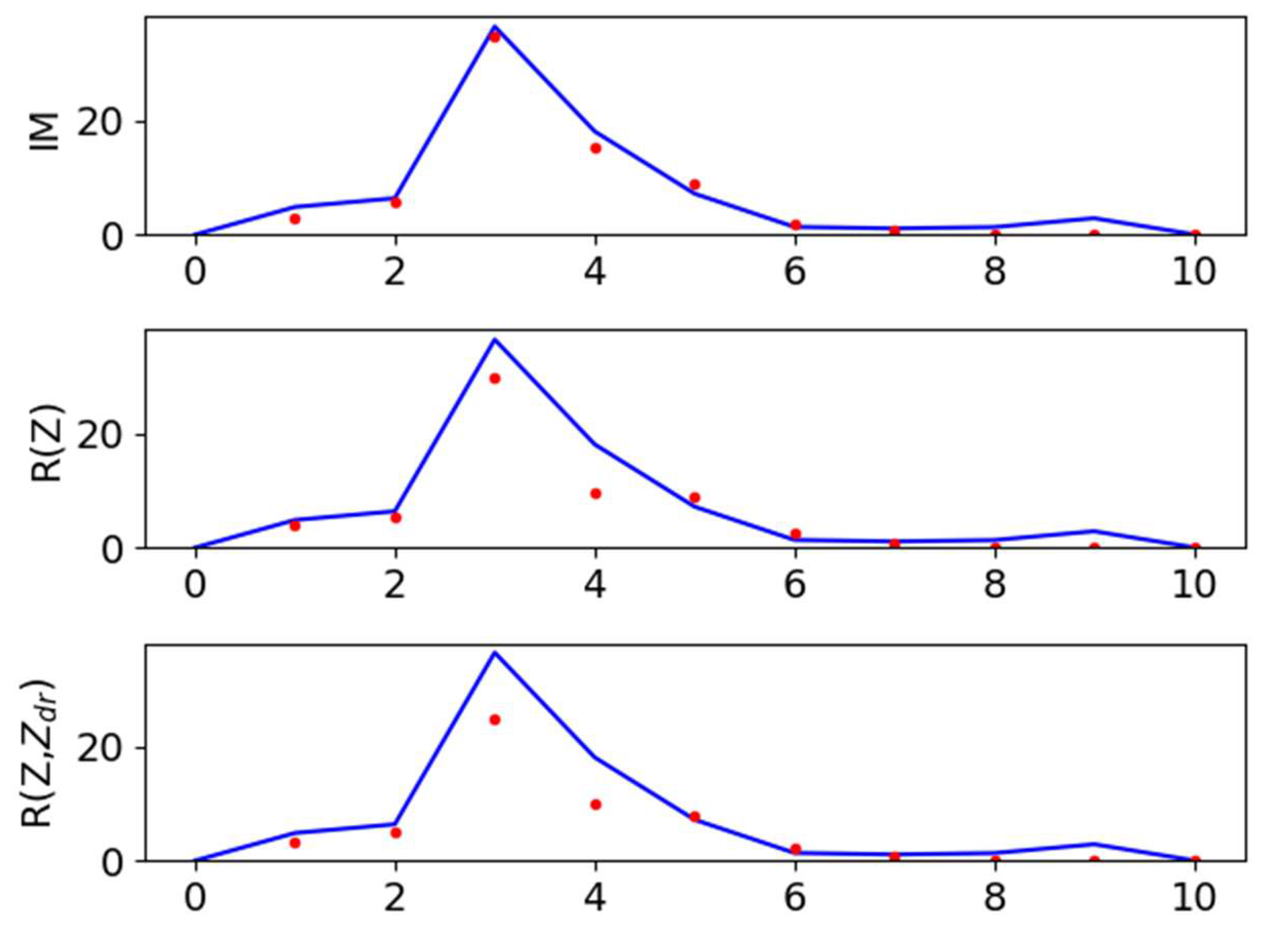
Figure 14 shows the results of rainfall rate estimation by IM, R(Zh), and R(Zh, Zdr). In general, the three retrievals well match the disdrometer observations with the correlation coefficient of 0.931, 0.932, and 0.937, respectively, while the MSE of IM is 95.2, about half that of R(Zh) and R(Zh, Zdr). However, all three algorithms tend to give an underestimation of the rainfall rate at the mature stage between 0800 and 0900 UTC. It is more evident from the one-hour rain accumulation (R1h), as shown in Figure 15. When R1h reaches its maximum at the third hour of the precipitating process, the bias (relative error) of IM is 1.63 mm (4.5%), comparing to 6.62 mm (18.2%) for R(Zh) and 11.69 mm (32.2%) for R(Zh, Zdr). It can be concluded that the inverse model gives some advantages over the power-law relations, particularly for the periods with high DSD variability.
6. Summary and Conclusions
In this paper, an inverse model for raindrop size distribution (DSD) retrieval has been designed and validated using observations from polarimetric radar and a two-dimensional video disdrometer.
First, the polarimetric variables, Zh, Zdr, and Kdp, were calculated via the T-matrix method to study the combined effects of the DSD and scattering properties of raindrops. Subsequently, a forward operator was obtained for each polarimetric variable by performing simulations for monodisperse raindrops under assumptions of ambient temperature, radar frequency, drop shape, and orientation. To yield an explicit form for the forward operator, the high-order polynomial approximation was utilized and optimized according to the mean square error test. The forward operator was then applied to assumed DSDs to generate a pseudo training dataset used by the inverse model. In addition, an empirical relation between the shape parameter and the slope parameter was used as an additional constraint to reduce the effect of instability in the forward operator when the maximum diameter was taken into account.
Secondly, a non-parametric estimator based on the nearest-neighborhood method was developed to map the polarimetric variables to DSD parameters. Since the input variables were on different scales, a normalization procedure was introduced to produce a zero-mean and unity-variance data matrix. The inverse model was then trained with regard to the mass-weighted mean diameter (Dm) and liquid water content (W), since these two microphysical quantities were important for the representation of DSD. Moreover, the characteristics of measurement errors of the polarimetric variables were investigated, leading to the conclusion that the error thresholds for Zh, Zdr, and Kdp are 0.2 dB, 0.1 dB, and 0.01 deg km−1, respectively.
Finally, the inverse model was validated by ten-year disdrometer data, and five-year joint observations from polarimetric radar. The results were also compared to an existing algorithm called a Bayesian approach. When the inverse model was applied to the simulated data, it generally yielded better agreement with the disdrometer observations when compared to the Bayesian approach. For real radar data, both the inverse model and Bayesian approach produced DSD retrievals with large uncertainties due to the measurement errors, noise, and sampling problems of the instruments. However, the inverse model still resulted in better DSD retrievals than the Bayesian approach in terms of mean square error, mean absolute error, relative square error, relative absolute error, and correlation coefficient. To make an operational use, the rainfall rate derived from the inverse model was compared to the power-law relations R(Zh) and R(Zh, Zdr), showing that the inverse model can improve rainfall rate estimation, particularly for the rainfall regimes with highly varied DSDs.
The inverse model may be extended to other DSD models, such as normalized Gamma model in Equation (5) and generalized Gamma model in Equation (10). In the normalized Gamma model, the normalized intercept is independent from the shape parameter in Equation (6), thus the retrieval procedure is equivalent to the ones proposed in this paper. In the generalized Gamma model, the moments play a key role in calculations of Zdr and Kdp/Zh via Equation (12). An inverse mode is then constructed to retrieve the moments within the generalized Gamma model.
The X-band radar has attracted increasing attentions in recent years, due to its low-cost, fine resolution, and high sensitivity to light rain. The inverse model may be adapted to the X-band frequency by considering three variables as a result of Mie effects, namely, specific attenuation (AH), differential attenuation (ADP), and differential phase shifts upon scattering (). Therefore, we can simultaneously obtain the rain-path attenuation correction and raindrop size distribution retrieval by using an iterative approach. Some pioneer work for X-band radars can be found in [19,20,77,78].
In the future, we will also apply the inverse model to the radar observations in the complex terrain [79]. With the intervention of the surface topography, the precipitation near the surface cannot be observed, giving a significant challenge on the DSD retrieval as well as rainfall rate estimation. Furthermore, we will investigate the rain characteristics in a tropical regime [72], with the DSD parameters derived by the inverse model.
Author Contributions
The work presented here was carried out in collaboration with all authors. G.W. designed and performed the calculation and wrote the manuscript. H.C., G.Z. and J.S. contributed to the reviewing and revising of the manuscript.
Funding
This work was supported in part by the China Scholarship Council, the National Natural Science Foundation of China (Grant No. 41605019), and the China Postdoctoral Science Foundation (Grant No. 2015M580123). The participation of H. Chen was also supported by the NRC Research Associateship Program.
Acknowledgments
We thank the two anonymous reviewers for their constructive comments.
Conflicts of Interest
The authors declare no conflict of interest.
References
- Seliga, T.A.; Bringi, V.N. Potential use of radar differential reflectivity measurements at orthogonal polarizations for measuring precipitation. J. Appl. Meteorol. 1976, 15, 69–76. [Google Scholar] [CrossRef]
- Seliga, T.A.; Bringi, V.N. Differential reflectivity and differential phase shift: Applications in radar meteorology. Radio Sci. 1978, 13, 271–275. [Google Scholar] [CrossRef]
- Keenan, T.; Glasson, K.; Cummings, F.; Bird, T.S.; Keeler, J.; Lutz, J. The BMRC/NCAR C-band polarimetric (C-POL) radar system. J. Atmos. Ocean. Technol. 1998, 15, 871–886. [Google Scholar] [CrossRef]
- Anagnostou, E.N.; Anagnostou, M.N.; Krajewski, W.F.; Kruger, A.; Miriovsky, B.J. High-resolution rainfall estimation from X-band polarimetric radar measurements. J. Hydrometeorol. 2004, 5, 110–128. [Google Scholar] [CrossRef]
- Bringi, V.N.; Chandrasekar, V. Polarimetric Doppler Weather Radar: Principles and Applications; Cambridge University Press: Cambridge, UK, 2001; p. 636. [Google Scholar]
- Doviak, R.J.; Zrnić, D.S. Doppler Radar and Weather Observations, 2nd ed.; Dover Publications, Inc.: Mineola, NY, USA, 2006; p. 562. [Google Scholar]
- Ulbrich, C.W. Natural variations in the analytical form of the raindrop size distribution. J. Clim. Appl. Meteorol. 1983, 22, 1764–1775. [Google Scholar] [CrossRef]
- Vivekanandan, J.; Zhang, G.; Brandes, E. Polarimetric Radar Estimators Based on a Constrained Gamma Drop Size Distribution Model. J. Appl. Meteorol. 2004, 43, 217–230. [Google Scholar] [CrossRef]
- Brandes, E.A.; Zhang, G.; Vivekanandan, J. Drop Size Distribution Retrieval with Polarimetric Radar: Model and Application. J. Appl. Meteorol. 2004, 43, 461–475. [Google Scholar] [CrossRef]
- Brandes, E.A.; Zhang, G.; Vivekanandan, J. An Evaluation of a Drop Distribution–Based Polarimetric Radar Rainfall Estimator. J. Appl. Meteorol. 2003, 42, 652–660. [Google Scholar] [CrossRef]
- Zhang, G.; Vivekanandan, J.; Brandes, E. A method for estimating rain rate and drop size distribution from polarimetric radar measurements. IEEE Trans. Geosci. Remote Sens. 2001, 39, 830–841. [Google Scholar] [CrossRef]
- Gorgucci, E.; Chandrasekar, V.; Bringi, V.N.; Scarchilli, G. Estimation of Raindrop Size Distribution Parameters from Polarimetric Radar Measurements. J. Atmos. Sci. 2002, 59, 2373–2384. [Google Scholar] [CrossRef] [Green Version]
- Willis, P.T. Functional fits to some observed drop size distributions and parameterization of rain. J. Atmos. Sci. 1984, 41, 1648–1661. [Google Scholar] [CrossRef]
- Illingworth, A.J.; Blackman, T.M. The Need to Represent Raindrop Size Spectra as Normalized Gamma Distributions for the Interpretation of Polarization Radar Observations. J. Appl. Meteorol. 2002, 41, 286–297. [Google Scholar] [CrossRef]
- Brandes, E.A.; Zhang, G.; Vivekanandan, J. Comparison of Polarimetric Radar Drop Size Distribution Retrieval Algorithms. J. Atmos. Ocean. Technol. 2004, 21, 584–598. [Google Scholar] [CrossRef]
- Anagnostou, M.N.; Anagnostou, E.N.; Vulpiani, G.; Montopoli, M.; Marzano, F.S.; Vivekanandan, J. Evaluation of X-Band Polarimetric-Radar Estimates of Drop-Size Distributions From Coincident S-Band Polarimetric Estimates and Measured Raindrop Spectra. IEEE Trans. Geosci. Remote Sens. 2008, 46, 3067–3075. [Google Scholar] [CrossRef]
- Bringi, V.N.; Huang, G.-J.; Chandrasekar, V.; Gorgucci, E. A Methodology for Estimating the Parameters of a Gamma Raindrop Size Distribution Model from Polarimetric Radar Data: Application to a Squall-Line Event from the TRMM/Brazil Campaign. J. Atmos. Ocean. Technol. 2002, 19, 633–645. [Google Scholar] [CrossRef] [Green Version]
- Bringi, V.N.; Chandrasekar, V.; Hubbert, J.; Gorgucci, E.; Randeu, W.L.; Schoenhuber, M. Raindrop Size Distribution in Different Climatic Regimes from Disdrometer and Dual-Polarized Radar Analysis. J. Atmos. Sci. 2003, 60, 354–365. [Google Scholar] [CrossRef]
- Anagnostou, M.N.; Kalogiros, J.; Marzano, F.S.; Anagnostou, E.N.; Montopoli, M.; Piccioti, E. Performance Evaluation of a New Dual-Polarization Microphysical Algorithm Based on Long-Term X-Band Radar and Disdrometer Observations. J. Hydrometeorol. 2013, 14, 560–576. [Google Scholar] [CrossRef]
- Kalogiros, J.; Anagnostou, M.N.; Anagnostou, E.N.; Montopoli, M.; Picciotti, E.; Marzano, F.S. Optimum Estimation of Rain Microphysical Parameters From X-Band Dual-Polarization Radar Observables. IEEE Trans. Geosci. Remote Sens. 2013, 51, 3063–3076. [Google Scholar] [CrossRef]
- Raupach, T.H.; Berne, A. Retrieval of the raindrop size distribution from polarimetric radar data using double-moment normalisation. Atmos. Meas. Tech. 2017, 10, 2573–2594. [Google Scholar] [CrossRef] [Green Version]
- Vulpiani, G.; Marzano, F.S.; Chandrasekar, V.; Berne, A.; Uijlenhoet, R. Polarimetric Weather Radar Retrieval of Raindrop Size Distribution by Means of a Regularized Artificial Neural Network. IEEE Trans. Geosci. Remote Sens. 2006, 44, 3262–3275. [Google Scholar] [CrossRef]
- Cao, Q.; Zhang, G.; Brandes, E.A.; Schuur, T.J. Polarimetric Radar Rain Estimation through Retrieval of Drop Size Distribution Using a Bayesian Approach. J. Appl. Meteorol. Climatol. 2010, 49, 973–990. [Google Scholar] [CrossRef]
- Yoshikawa, E.; Chandrasekar, V.; Ushio, T.; Matsuda, T. A Bayesian Approach for Integrated Raindrop Size Distribution (DSD) Retrieval on an X-Band Dual-Polarization Radar Network. J. Atmos. Ocean. Technol. 2016, 33, 377–389. [Google Scholar] [CrossRef]
- Cao, Q.; Zhang, G.; Xue, M. A Variational Approach for Retrieving Raindrop Size Distribution from Polarimetric Radar Measurements in the Presence of Attenuation. J. Appl. Meteorol. Climatol. 2013, 52, 169–185. [Google Scholar] [CrossRef] [Green Version]
- Wen, G.; Xiao, H.; Yang, H.; Bi, Y.; Xu, W. Characteristics of summer and winter precipitation over northern China. Atmos. Res. 2017, 197, 390–406. [Google Scholar] [CrossRef]
- Kruger, A.; Krajewski, W.F. Two-Dimensional Video Disdrometer: A Description. J. Atmos. Ocean. Technol. 2002, 19, 602–617. [Google Scholar] [CrossRef]
- Löffler-Mang, M.; Joss, J. An Optical Disdrometer for Measuring Size and Velocity of Hydrometeors. J. Atmos. Ocean. Technol. 2000, 17, 130–139. [Google Scholar] [CrossRef]
- Feingold, G.; Levin, Z. The Lognormal Fit to Raindrop Spectra from Frontal Convective Clouds in Israel. J. Clim. Appl. Meteorol. 1986, 25, 1346–1363. [Google Scholar] [CrossRef] [Green Version]
- Marshall, J.S.; Palmer, W.M.K. The distribution of raindrops with size. J. Meteorol. 1948, 5, 165–166. [Google Scholar] [CrossRef]
- Maguire, W.B., II; Avery, S.K. Retrieval of Raindrop Size Distributions Using Two Doppler Wind Profilers: Model Sensitivity Testing. J. Appl. Meteorol. 1994, 33, 1623–1635. [Google Scholar] [CrossRef] [Green Version]
- Schönhuber, M.; Lammer, G.; Randeu, W. One decade of imaging precipitation measurement by 2D-video-distrometer. Adv. Geosci. 2007, 10, 85–90. [Google Scholar] [CrossRef] [Green Version]
- Kumjian, M.R.; Ryzhkov, A.V. The Impact of Size Sorting on the Polarimetric Radar Variables. J. Atmos. Sci. 2012, 69, 2042–2060. [Google Scholar] [CrossRef]
- Testud, J.; Oury, S.; Black, R.A.; Amayenc, P.; Dou, X. The Concept of “Normalized” Distribution to Describe Raindrop Spectra: A Tool for Cloud Physics and Cloud Remote Sensing. J. Appl. Meteorol. 2001, 40, 1118–1140. [Google Scholar] [CrossRef]
- Sekhon, R.S.; Srivastava, R.C. Snow Size Spectra and Radar Reflectivity. J. Atmos. Sci. 1970, 27, 299–307. [Google Scholar] [CrossRef] [Green Version]
- Thurai, M.; Bringi, V.N. Application of the Generalized Gamma Model to Represent the Full Rain Drop Size Distribution Spectra. J. Appl. Meteorol. Climatol. 2018. [Google Scholar] [CrossRef]
- Lee, G.W.; Zawadzki, I.; Szyrmer, W.; Sempere-Torres, D.; Uijlenhoet, R. A General Approach to Double-Moment Normalization of Drop Size Distributions. J. Appl. Meteorol. 2004, 43, 264–281. [Google Scholar] [CrossRef]
- Brandes, E.A.; Zhang, G.; Vivekanandan, J. Experiments in Rainfall Estimation with a Polarimetric Radar in a Subtropical Environment. J. Appl. Meteorol. 2002, 41, 674–685. [Google Scholar] [CrossRef]
- Atlas, D.; Srivastava, R.; Sekhon, R.S. Doppler radar characteristics of precipitation at vertical incidence. Rev. Geophys. 1973, 11, 1–35. [Google Scholar] [CrossRef]
- Pruppacher, H.R.; Beard, K.V. A wind tunnel investigation of the internal circulation and shape of water drops falling at terminal velocity in air. Q. J. R. Meteorol. Soc. 1970, 96, 247–256. [Google Scholar] [CrossRef]
- Helmus, J.; Collis, S. The Python ARM Radar Toolkit (Py-ART), a library for working with weather radar data in the Python programming language. J. Open Res. Softw. 2016, 4, e25. [Google Scholar] [CrossRef]
- Heistermann, M.; Collis, S.; Dixon, M.J.; Giangrande, S.; Helmus, J.J.; Kelley, B.; Koistinen, J.; Michelson, D.B.; Peura, M.; Pfaff, T.; et al. The Emergence of Open-Source Software for the Weather Radar Community. Bull. Am. Meteorol. Soc. 2015, 96, 117–128. [Google Scholar] [CrossRef]
- Lakshmanan, V.; Karstens, C.; Krause, J.; Tang, L. Quality Control of Weather Radar Data Using Polarimetric Variables. J. Atmos. Ocean. Technol. 2014, 31, 1234–1249. [Google Scholar] [CrossRef]
- Lakshmanan, V.; Jian, Z. Censoring Biological Echoes in Weather Radar Images. In Proceedings of the Sixth International Conference on FSKD ‘09 Fuzzy Systems and Knowledge Discovery, Tianjin, China, 14–16 August 2009; pp. 491–495. [Google Scholar]
- Lakshmanan, V.; Smith, T.; Stumpf, G.; Hondl, K. The Warning Decision Support System–Integrated Information. Weather Forecast. 2007, 22, 596–612. [Google Scholar] [CrossRef]
- Vulpiani, G.; Montopoli, M.; Passeri, L.D.; Gioia, A.G.; Giordano, P.; Marzano, F.S. On the Use of Dual-Polarized C-Band Radar for Operational Rainfall Retrieval in Mountainous Areas. J. Appl. Meteorol. Climatol. 2012, 51, 405–425. [Google Scholar] [CrossRef]
- Klazura, G.E.; Imy, D.A. A Description of the Initial Set of Analysis Products Available from the NEXRAD WSR-88D System. Bull. Am. Meteorol. Soc. 1993, 74, 1293–1312. [Google Scholar] [CrossRef]
- Crum, T.; Smith, S.; Chrisman, J.; Vogt, R.; Istok, M.; Hall, R.; Saffle, B. WSR-88D Radar Projects: 2013 Update. In Proceedings of the 29th Conference on Environmental Information Processing Technologies, Austin, TX, USA, 9 January 2013. [Google Scholar]
- Nešpor, V.; Krajewski, W.F.; Kruger, A. Wind-Induced Error of Raindrop Size Distribution Measurement Using a Two-Dimensional Video Disdrometer. J. Atmos. Ocean. Technol. 2000, 17, 1483–1492. [Google Scholar] [CrossRef]
- Wen, G.; Protat, A.; May, P.T.; Wang, X.; Moran, W. A Cluster-Based Method for Hydrometeor Classification Using Polarimetric Variables. Part I: Interpretation and Analysis. J. Atmos. Ocean. Technol. 2015, 32, 1320–1340. [Google Scholar] [CrossRef]
- Straka, J.M.; Zrnić, D.S.; Ryzhkov, A.V. Bulk hydrometeor classification and quantification using polarimetric radar data: Synthesis of relations. J. Appl. Meteorol. 2000, 39, 1341–1372. [Google Scholar] [CrossRef]
- Mishchenko, M.I. Calculation of the amplitude matrix for a nonspherical particle in a fixed orientation. Appl. Opt. 2000, 39, 1026–1031. [Google Scholar] [CrossRef] [PubMed]
- Waterman, P.C. Symmetry, unitarity, and geometry in electromagnetic scattering. Phys. Rev. D 1971, 3, 825. [Google Scholar] [CrossRef]
- Ray, P.S. Broadband complex refractive indices of ice and water. Appl. Opt. 1972, 11, 1836. [Google Scholar] [CrossRef] [PubMed]
- Thurai, M.; Bringi, V.; May, P. Drop shape studies in rain using 2-D video disdrometer and dual-wavelength, polarimetric CP-2 radar measurements in south-east Queensland, Australia. In Proceedings of the 34th Conference on Radar Meteorology, Williamsburg, VA, USA, 5–9 October 2009; American Meteor Society Press: Geneseo, NY, USA, 2009. [Google Scholar]
- Huang, G.-J.; Bringi, V.N.; Thurai, M. Orientation Angle Distributions of Drops after an 80-m Fall Using a 2D Video Disdrometer. J. Atmos. Ocean. Technol. 2008, 25, 1717–1723. [Google Scholar] [CrossRef]
- Scarchilli, G.; Gorgucci, V.; Chandrasekar, V.; Dobaie, A. Self-consistency of polarization diversity measurement of rainfall. IEEE Trans. Geosci. Remote Sens. 1996, 34, 22–26. [Google Scholar] [CrossRef] [Green Version]
- Atlas, D.; Ulbrich, C. Drop size spectra and integral remote sensing parameters in the transition from convective to stratiform rain. Geophys. Res. Lett. 2006, 33. [Google Scholar] [CrossRef] [Green Version]
- Moisseev, D.N.; Chandrasekar, V. Examination of the μ–Λ Relation Suggested for Drop Size Distribution Parameters. J. Atmos. Ocean. Technol. 2007, 24, 847–855. [Google Scholar] [CrossRef]
- Cao, Q.; Zhang, G. Errors in Estimating Raindrop Size Distribution Parameters Employing Disdrometer and Simulated Raindrop Spectra. J. Appl. Meteorol. Climatol. 2009, 48, 406–425. [Google Scholar] [CrossRef]
- Zhang, G.; Vivekanandan, J.; Brandes, E.A.; Meneghini, R.; Kozu, T. The Shape–Slope Relation in Observed Gamma Raindrop Size Distributions: Statistical Error or Useful Information? J. Atmos. Ocean. Technol. 2003, 20, 1106–1119. [Google Scholar] [CrossRef]
- Williams, C.R.; Bringi, V.N.; Carey, L.D.; Chandrasekar, V.; Gatlin, P.N.; Haddad, Z.S.; Meneghini, R.; Munchak, S.J.; Nesbitt, S.W.; Petersen, W.A.; et al. Describing the Shape of Raindrop Size Distributions Using Uncorrelated Raindrop Mass Spectrum Parameters. J. Appl. Meteorol. Climatol. 2014, 53, 1282–1296. [Google Scholar] [CrossRef]
- Cao, Q.; Zhang, G.; Brandes, E.; Schuur, T.; Ryzhkov, A.; Ikeda, K. Analysis of video disdrometer and polarimetric radar data to characterize rain microphysics in Oklahoma. J. Appl. Meteorol. Climatol. 2008, 47, 2238–2255. [Google Scholar] [CrossRef]
- Härter, F.P.; de Campos Velho, H.F. New approach to applying neural network in nonlinear dynamic model. Appl. Math. Model. 2008, 32, 2621–2633. [Google Scholar] [CrossRef]
- Lemm, J.C. Bayesian Field Theory; JHU Press: Baltimore, MD, USA, 2003. [Google Scholar]
- Teboul, S.; Blanc-Feraud, L.; Aubert, G.; Barlaud, M. Variational approach for edge-preserving regularization using coupled PDEs. IEEE Trans. Image Process. 1998, 7, 387–397. [Google Scholar] [CrossRef] [PubMed]
- Wen, G.; Protat, A.; May, P.T.; Moran, W.; Dixon, M. A Cluster-Based Method for Hydrometeor Classification Using Polarimetric Variables. Part II: Classification. J. Atmos. Ocean. Technol. 2016, 33, 45–60. [Google Scholar] [CrossRef]
- Prat, O.P.; Barros, A.P.; Testik, F.Y. On the Influence of Raindrop Collision Outcomes on Equilibrium Drop Size Distributions. J. Atmos. Sci. 2012, 69, 1534–1546. [Google Scholar] [CrossRef]
- D’Adderio, L.P.; Porcù, F.; Tokay, A. Identification and Analysis of Collisional Breakup in Natural Rain. J. Atmos. Sci. 2015, 72, 3404–3416. [Google Scholar] [CrossRef]
- D’Adderio, L.P.; Porcù, F.; Tokay, A. Evolution of drop size distribution in natural rain. Atmos. Res. 2018, 200, 70–76. [Google Scholar] [CrossRef]
- Smith, P.L.; Kliche, D.V.; Johnson, R.W. The Bias and Error in Moment Estimators for Parameters of Drop Size Distribution Functions: Sampling from Gamma Distributions. J. Appl. Meteorol. Climatol. 2009, 48, 2118–2126. [Google Scholar] [CrossRef]
- Bringi, V.N.; Williams, C.R.; Thurai, M.; May, P.T. Using dual-polarized radar and dual-frequency profiler for DSD characterization: A case study from Darwin, Australia. J. Atmos. Ocean. Technol. 2009, 26, 2107–2122. [Google Scholar] [CrossRef]
- Sinnott, R.W. Virtues of the Haversine. Sky Telesc. 1984, 68, 159. [Google Scholar]
- Kozu, T.; Nakamura, K. Rainfall Parameter Estimation from Dual-Radar Measurements Combining Reflectivity Profile and Path-integrated Attenuation. J. Atmos. Ocean. Technol. 1991, 8, 259–270. [Google Scholar] [CrossRef] [Green Version]
- Chen, H.; Chandrasekar, V.; Bechini, R. An improved dual-polarization radar rainfall algorithm (DROPS2. 0): Application in NASA IFloodS field campaign. J. Hydrometeorol. 2017, 18, 917–937. [Google Scholar] [CrossRef]
- Ryzhkov, A.V.; Giangrande, S.E.; Schuur, T.J. Rainfall Estimation with a Polarimetric Prototype of WSR-88D. J. Appl. Meteorol. 2005, 44, 502–515. [Google Scholar] [CrossRef]
- Park, S.-G.; Bringi, V.N.; Chandrasekar, V.; Maki, M.; Iwanami, K. Correction of Radar Reflectivity and Differential Reflectivity for Rain Attenuation at X Band. Part I: Theoretical and Empirical Basis. J. Atmos. Ocean. Technol. 2005, 22, 1621–1632. [Google Scholar] [CrossRef] [Green Version]
- Chen, H.; Chandrasekar, V.; Yoshikawa, E. A rain drop size distribution (DSD) retrieval algorithm for CASA DFW urban radar network. In Proceedings of the 36th Conference on Radar Meteorology, Denver, CO, USA, 16–20 September 2013. [Google Scholar]
- Cifelli, R.; Chandrasekar, V.; Chen, H.; Johnson, L.E. High resolution radar quantitative precipitation estimation in the San Francisco Bay area: Rainfall monitoring for the urban environment. J. Meteorol. Soc. Jpn. 2018, 96, 141–155. [Google Scholar] [CrossRef]
Figure 1.
Characteristics of polarimetric variables simulated by a T-matrix method: (a) Zh vs. Zdr; (b) Zh vs. Kdp; and (c) Zdr and Kdp. Note that Zh and Zdr are on a logarithmic scale with units of dBZ and dB, respectively.
Figure 1.
Characteristics of polarimetric variables simulated by a T-matrix method: (a) Zh vs. Zdr; (b) Zh vs. Kdp; and (c) Zdr and Kdp. Note that Zh and Zdr are on a logarithmic scale with units of dBZ and dB, respectively.

Figure 2.
The forward operators and polynomial fit for: (a) radar reflectively at the horizontal polarization (Zh); (b) radar reflectivity at the vertical polarization (Zv); and (c) specific differential phase (Kdp).
Figure 2.
The forward operators and polynomial fit for: (a) radar reflectively at the horizontal polarization (Zh); (b) radar reflectivity at the vertical polarization (Zv); and (c) specific differential phase (Kdp).

Figure 3.
The mean square errors for polynomial fits for the forward operator of: (a) Zh; (b) Zv; and (c) Kdp. The various colors represent basis orders ranging from 3 to 7.
Figure 3.
The mean square errors for polynomial fits for the forward operator of: (a) Zh; (b) Zv; and (c) Kdp. The various colors represent basis orders ranging from 3 to 7.

Figure 4.
Scatterplots of the polarimetric variables calculated via an integral equation (abscissa axis) and via polynomial fitted relation (ordinate axis): (a) Zh; (b) Zv; and (c) Kdp. The red line is a reference for the abscissa axis equal to the ordinate axis.
Figure 4.
Scatterplots of the polarimetric variables calculated via an integral equation (abscissa axis) and via polynomial fitted relation (ordinate axis): (a) Zh; (b) Zv; and (c) Kdp. The red line is a reference for the abscissa axis equal to the ordinate axis.

Figure 5.
The - relation for the disdrometer data. The blue dots are the and parameters obtained by a truncated Gamma method [8]. The red curve is a second-order polynomial fit for the data, and the green curve is (7) in [63].

Figure 6.
Simulations of Zdr and Kdp/Zh on linear scales: (a) the colored curves represent a number of fixed ; and (b) the colored curves represent a number of fixed Dmax.
Figure 6.
Simulations of Zdr and Kdp/Zh on linear scales: (a) the colored curves represent a number of fixed ; and (b) the colored curves represent a number of fixed Dmax.

Figure 7.
An example of DSD retrieval for illustration of the difference between the real DSD and Gamma model. The blue dots are the DSD observed by the disdrometer at 02:05 UTC on 27 August 2006. The red curve is the Gamma fit for the disdrometer data with the truncated moment method. The green curve is the DSD retrieved by the nearest neighborhood method.

Figure 8.
The mean square errors of (a) Dm and (b) W, associated with the model complexity. Note the abscissa of (a) is the number of neighbors used in the nearest neighborhood model for and in (b) is the complexity of the model for Dmax.
Figure 8.
The mean square errors of (a) Dm and (b) W, associated with the model complexity. Note the abscissa of (a) is the number of neighbors used in the nearest neighborhood model for and in (b) is the complexity of the model for Dmax.

Figure 9.
Error characteristics of Dm and W associated with the bias of Zh, Zdr, and Kdp, respectively, in the disdrometer dataset. The blue curves represent the positive biases, while the red curves are the negative ones.
Figure 9.
Error characteristics of Dm and W associated with the bias of Zh, Zdr, and Kdp, respectively, in the disdrometer dataset. The blue curves represent the positive biases, while the red curves are the negative ones.

Figure 10.
Comparison between the disdrometer data and DSD retrieved by the simulated data: (a) Dm by the inverse model; (b) W by the inverse model; (c) Dm by the Bayesian approach; and (d) W by the Bayesian approach. The red curve indicates the abscissa is identical to the ordinate.
Figure 10.
Comparison between the disdrometer data and DSD retrieved by the simulated data: (a) Dm by the inverse model; (b) W by the inverse model; (c) Dm by the Bayesian approach; and (d) W by the Bayesian approach. The red curve indicates the abscissa is identical to the ordinate.

Figure 11.
Same as Figure 10, but for real radar data.
Figure 11.
Same as Figure 10, but for real radar data.

Figure 12.
Comparison of the DSD moments retrieved by the inverse model: (a) the zeroth-moment; (b) the second-moment; (c) the fourth-moment; and (d) the sixth-moment.
Figure 12.
Comparison of the DSD moments retrieved by the inverse model: (a) the zeroth-moment; (b) the second-moment; (c) the fourth-moment; and (d) the sixth-moment.

Figure 13.
Time-series data of the polarimetric variables: (a) Zh (dBZ); (b) Zdr (dB); and (c) Kdp (deg km−1). The data were collected between 0614 and 1519 UTC on 8 June 2014. The blue curve indicates disdrometer observations, and the red dots are the radar measurements.
Figure 13.
Time-series data of the polarimetric variables: (a) Zh (dBZ); (b) Zdr (dB); and (c) Kdp (deg km−1). The data were collected between 0614 and 1519 UTC on 8 June 2014. The blue curve indicates disdrometer observations, and the red dots are the radar measurements.

Figure 14.
Same as Figure 13, but for rainfall rate retrieved by: the inverse model (top); R(Z) (middle); and R(Z, Zdr) (bottom).
Figure 14.
Same as Figure 13, but for rainfall rate retrieved by: the inverse model (top); R(Z) (middle); and R(Z, Zdr) (bottom).

Figure 15.
Same as Figure 14, but for one-hour rainfall accumulation.
Figure 15.
Same as Figure 14, but for one-hour rainfall accumulation.


Table 1.
Means, standard deviations (STD), minima (min), and maxima (max) for quantities derived from the disdrometer observations. Zh is the radar reflectivity on a logarithmic scale, Zdr is the differential reflectivity on a logarithmic scale, Kdp is the specific differential phase, Dm is the mass-weighted mean diameter, W is the liquid water content, and R is the rainfall rate at the surface. Note the means and standard deviations of Zh and Zdr are calculated on a linear scale, and then transferred to a logarithmic scale.
| Zh (dBZ) | Zdr (dB) | Kdp (deg/km) | Dm (mm) | W (g/m3) | R (mm/h) | |
|---|---|---|---|---|---|---|
| Mean | 36.8 | 0.67 | 0.076 | 1.30 | 0.314 | 5.4 |
| STD | 7.0 | 0.60 | 0.251 | 0.40 | 0.986 | 16.1 |
| Min | 3.6 | 0 | 0 | 0.36 | 0.0004 | 0.1 |
| Max | 58.2 | 5.87 | 7.031 | 5.74 | 35.031 | 479.5 |
Table 2.
Coefficients of the polynomial fits for Zh, Zv, and Kdp and metrics for the polynomial fits. MSE, mean square error; RE, relative error; CC, correlation coefficient.
Table 2.
Coefficients of the polynomial fits for Zh, Zv, and Kdp and metrics for the polynomial fits. MSE, mean square error; RE, relative error; CC, correlation coefficient.
| b | p | a0 | a1 | a2 | a3 | a4 | Bias | MSE | RE | CC | |
|---|---|---|---|---|---|---|---|---|---|---|---|
| Zh | 6 | 3 | 1.004 | −0.020 | 0.021 | −0.417 | 28.965 | 1 | |||
| Zv | 6 | 4 | 0.998 | 0.028 | −0.055 | −0.265 | 13.420 | 1 | |||
| Kdp | 4 | 4 | 1 |
Table 3.
Mean square error (MSE), mean absolute error, relative square error (RSE), relative absolute error (RAE), and correlation coefficient (CC) for Dm and W obtained by the inverse model (IM) and Bayesian approach (BA).
Table 3.
Mean square error (MSE), mean absolute error, relative square error (RSE), relative absolute error (RAE), and correlation coefficient (CC) for Dm and W obtained by the inverse model (IM) and Bayesian approach (BA).
| MSE | MAE | RSE | RAE | CC | |
|---|---|---|---|---|---|
| Dm (IM) | 0.030 | 0.124 | 0.183 | 0.405 | 0.917 |
| Dm (BA) | 0.091 | 0.239 | 0.552 | 0.782 | 0.821 |
| W (IM) | 0.113 | 0.062 | 0.128 | 0.178 | 0.963 |
| W (BA) | 0.218 | 0.090 | 0.246 | 0.257 | 0.934 |
Table 4.
Same as Table 3, but for real radar data.
Table 4.
Same as Table 3, but for real radar data.
| MSE | MAE | RSE | RAE | CC | |
|---|---|---|---|---|---|
| Dm (IM) | 0.062 | 0.181 | 0.747 | 0.882 | 0.504 |
| Dm (BA) | 0.123 | 0.270 | 1.470 | 1.315 | 0.463 |
| W (IM) | 1.081 | 0.300 | 0.515 | 0.492 | 0.705 |
| W (BA) | 1.167 | 0.317 | 0.557 | 0.522 | 0.679 |
Table 5.
Root mean square error (RMSE), mean absolute error (MAE), root relative square error (RRSE), relative absolute error (RAE), and correlation coefficient (CC) for the zeroth, second, fourth, and sixth moments, respectively.
Table 5.
Root mean square error (RMSE), mean absolute error (MAE), root relative square error (RRSE), relative absolute error (RAE), and correlation coefficient (CC) for the zeroth, second, fourth, and sixth moments, respectively.
| RMSE | MAE | RRSE | RAE | CC | |
|---|---|---|---|---|---|
| Zeroth | 14,373.8 | 4602.5 | 1.233 | 0.986 | 0.651 |
| Second | 2453.2 | 660.7 | 0.746 | 0.497 | 0.696 |
| Fourth | 2469.1 | 734.6 | 0.721 | 0.480 | 0.714 |
| Sixth | 16,391.1 | 3800.8 | 0.855 | 0.455 | 0.659 |
© 2018 by the authors. Licensee MDPI, Basel, Switzerland. This article is an open access article distributed under the terms and conditions of the Creative Commons Attribution (CC BY) license (http://creativecommons.org/licenses/by/4.0/).
Share and Cite
MDPI and ACS Style
Wen, G.; Chen, H.; Zhang, G.; Sun, J. An Inverse Model for Raindrop Size Distribution Retrieval with Polarimetric Variables. Remote Sens. 2018, 10, 1179. https://doi.org/10.3390/rs10081179
AMA Style
Wen G, Chen H, Zhang G, Sun J. An Inverse Model for Raindrop Size Distribution Retrieval with Polarimetric Variables. Remote Sensing. 2018; 10(8):1179. https://doi.org/10.3390/rs10081179
Chicago/Turabian StyleWen, Guang, Haonan Chen, Guifu Zhang, and Jiming Sun. 2018. "An Inverse Model for Raindrop Size Distribution Retrieval with Polarimetric Variables" Remote Sensing 10, no. 8: 1179. https://doi.org/10.3390/rs10081179
Note that from the first issue of 2016, this journal uses article numbers instead of page numbers. See further details here.