Urban Change Detection Based on Dempster–Shafer Theory for Multitemporal Very High-Resolution Imagery

Abstract

Fusing multiple change detection results has great potentials in dealing with the spectral variability in multitemporal very high-resolution (VHR) remote sensing images. However, it is difficult to solve the problem of uncertainty, which mainly includes the inaccuracy of each candidate change map and the conflicts between different results. Dempster–Shafer theory (D–S) is an effective method to model uncertainties and combine multiple evidences. Therefore, in this paper, we proposed an urban change detection method for VHR images by fusing multiple change detection methods with D–S evidence theory. Change vector analysis (CVA), iteratively reweighted multivariate alteration detection (IRMAD), and iterative slow feature analysis (ISFA) were utilized to obtain the candidate change maps. The final change detection result is generated by fusing the three evidences with D–S evidence theory and a segmentation object map. The experiment indicates that the proposed method can obtain the best performance in detection rate, false alarm rate, and comprehensive indicators.

1. Introduction

Remote sensing imagery has been one of the major data sources for studying human development and monitoring ecosystems [1,2,3,4,5,6]. When multitemporal remote sensing images covering the same areas are able to be obtained, it is a matter of course to analyze where the landscape conditions have changed and what types the changes are. Therefore, change detection is one of the earliest and most important interpretation approaches for remote sensing technology [7,8,9]. Dynamic analysis of landscape variation by change detection is extremely useful in many applications, such land-use/land-cover change, urban expansion, ecosystem monitoring, and resource management [10,11,12,13,14,15,16,17,18].

In the literatures, numerous studies have been proposed for change detection, which can be categorized into three classes [19]: (1) direct comparison, which calculates the difference between the original spectral features, such as image difference, image ratio, and change vector analysis [9,20,21,22]; (2) image transformation, which obtains the change information by transforming the original data into new discriminant features, such as principle component analysis, multivariate alteration detection (MAD), and slow feature analysis (SFA) [23,24,25]; (3) classification based method, which analyzes the “from-to” change types by comparing the classification maps or classifying the multitemporal combinations, such as post-classification method and direct classification [26,27].

With the development of very high-resolution (VHR) remote sensing technology, multitemporal VHR images are much easier to obtain and are widely used in building change detection, disaster assessment, and detailed land-cover change monitoring [28,29,30,31,32,33]. In order to take advantage of the abundant textual information and detailed spatial relationship [34,35,36], various studies have been proposed for multitemporal VHR data [32]. We can group them into two categories: (1) object-oriented change detection, which utilizes the object as the process unit to improve the completeness and accuracy of the final result [19,37,38]; (2) change detection fusing spatial features, which takes into consideration the texture, shape, and topology features in the process of change analysis [28,39,40].

In most previous works for multitemporal VHR data, one specific change detection method was utilized to obtain the change intensity, measuring the probability to be changed. However, with the increase of spatial resolution, the high reflectance variability within individual objects in urban areas also increases, so that no single method can obtain a satisfactory performance. When fusing multiple change detection results, the uncertainty will be the main problem, which contains the inaccuracy of each result and the conflict between different decisions.

Dempster–Shafer Theory (D–S) is a decision theory effectively fusing multiple evidences from different sources [41]. One important advantage of D–S theory is that it can provide explicit estimations of uncertainty between different evidences from different data sources [42,43]. Thus, the fusion of change detection results by D–S theory aims to improve the reliability of decisions by taking advantage of complementary information while decreasing their uncertainty [44].

In this paper, we proposed an urban change detection method for VHR remote sensing images by fusing multiple change detection methods with D–S theory and segmentation objects. Firstly, the multitemporal VHR images were stacked for object segmentation. Since change vector analysis (CVA) [20], iteratively reweighted multivariate alteration detection (IRMAD) [24], and iterative slow feature analysis (ISFA) [23] are all classical unsupervised methods and perform well in urban change detection, they were then implemented to obtain three candidate change maps, respectively. Finally, these three change maps were fused based on the object map and D–S theory to obtain the final result.

The contribution of this paper is in proposing a framework of fusing multiple change detection methods by D–S theory considering the uncertainty of each binary candidate result. Although there have been numerous studies about change detection, it is hard to obtain a satisfactory result with a single method due to the complexity of the urban environment in VHR images. When combining multiple change detection results, few studies take the uncertainty, which mainly includes the inaccuracy of each candidate change map and the conflicts between different results, into consideration. In our paper, the proposed fusion method by D–S theory has the ability to explore the uncertainty among different results and to generate a more accurate change map.

The rest of this paper is organized as follows. Section 2 details the proposed change detection method. The experiments are addressed in Section 3. Section 4 shows the detailed discussion. Finally, Section 5 draws the conclusion.

2. Methodology

In this section, we elaborate how to fuse the results of different change detection methods with D–S theory to improve the performance for multitemporal VHR images. The whole procedure of the proposed method is shown in Figure 1. The main steps are as follows:

(1)

Obtain the object map by the segmentation of stacked multitemporal VHR images;

(2)

Implement three change detection methods (CVA, ISFA, and IRMAD) to get change intensity, and utilize OTSU thresholding method to obtain the candidate change maps;

(3)

Fuse the three candidate change maps by the object map and D–S theory to obtain the final object-oriented change map.

2.1. Segmentation

VHR remote sensing imagery can provide detailed and abundant spatial information. However, the high spectral variability within individual objects have challenged the traditional pixelwise image interpretation [19]. Object-oriented image analysis (OOIA) is a good idea to deal with the problem of spectral variability and has the ability to keep the object completeness.

For change detection with multitemporal VHR images, it is important to maintain the temporal consistency of objects, which means the pixels within one object are all changed or unchanged. In this paper, we firstly stacked the multitemporal images and implemented multiresolution segmentation to obtain the object map [45]. Multiresolution segmentation (MRS) is an effective segmentation algorithm, which forms homogenous objects by a bottom-up region merging. The software of eCognition Developer was utilized to employ MRS in this study.

2.2. Change Detection

Due to the complexity of multitemporal VHR images, no single change detection can obtain a very accurate result. Therefore, in this paper, we utilized three effective change detection methods and fused their results by D–S theory. We call them “component methods”. The three component methods are CVA, IRMAD, and ISFA, since they are all effective unsupervised change detection methods.

CVA is a classical change detection method and has been the foundation of numerous researches [20]. The change vector was obtained by differencing the spectral values of corresponding bands, and the change intensity was calculated with the Euclidean distance of the change vector as follows:

$$d=\left|\right|\mathit{y}-\mathit{x}|{|}_2$$

(1)

where $\mathit{x}$ and $\mathit{y}$ indicate the spectral vectors and $d$ means the change intensity.

IRMAD is an improved version of the MAD algorithm [24]. It assigns high weights to the unchanged pixels during the iterations so as to reduce the negative effect of changed pixels in the feature space learning [24,46,47]. After the convergence of IRMAD is achieved, the chi-squared distance of the transformed features is used as the change intensity [24]. For IRMAD, the transformation vectors $\mathit{a}$ and $\mathit{b}$ should satisfy the following optimization objective:

$${\arg }_{\mathit{a},\mathit{b}}\max \left\{\mathrm{Var}\left({\mathit{a}}^T\mathit{x}-{\mathit{b}}^T\mathit{y}\right)\right\},\mathrm{s}.\mathrm{t}.\mathrm{Var}\left({\mathit{a}}^T\mathit{x}\right)=1, \mathrm{Var}\left({\mathit{b}}^T\mathit{y}\right)=1$$

(2)

The change intensity of IRMAD is calculated by the chi-squared distance as

$$d={\displaystyle \sum }_k{\left(\frac{{\left({\mathit{a}}^T\mathit{x}-{\mathit{b}}^T\mathit{y}\right)}^k}{{\sigma }^k}\right)}^2$$

(3)

where ${\sigma }^k$ indicates the variance of $k_{th}$ feature band.

ISFA is an iterative improvement of the SFA change detection method [23]. SFA can extract the temporal invariant features from multitemporal images and reduce the spectral variance between unchanged landscapes [48]. In this way, the real changes are anomalous from the invariant features and can be well separated in the feature differences [49]. ISFA is proposed to consider more unchanged pixels in feature learning during the iterations by assigning high weights to unchanged pixels and almost zero weights to the changed pixels [23]. For ISFA, the transformation vectors $\mathit{w}$ should satisfy the following optimization objective:

$${\arg }_{\mathit{w}}\min \left\{{\mathit{w}}^T\mathit{x}-{\mathit{w}}^T\mathit{y}\right\}$$

(4)

where the transformed features should be under the constraints of zero mean, unit variance, and decorrelation. The chi-squared distance are also used to calculate the change intensity [23]:

$$d={\displaystyle \sum }_k{\left(\frac{{\left({\mathit{w}}^T\mathit{x}-{\mathit{w}}^T\mathit{y}\right)}^k}{{\sigma }^k}\right)}^2$$

(5)

where ${\sigma }^k$ also indicates the variance of $k_{th}$ SFA feature band.

After the change intensity were obtained, the automatic thresholding method was utilized to generate the binary change maps. OTSU was selected as the thresholding method due to its effectiveness and simplicity [23,48]. In order to test the effectiveness of OTSU automatic thresholding algorithm, we also evaluated the results with different thresholding methods, including K-means two-class clustering [25] and expectation maximization (EM) thresholding [50]. The maximum accuracies by traversing all possible thresholds are also shown as comparisons.

2.3. Fusion with D–S Theory

Due to the complexity of VHR images, it is evident that no single method can provide a consistent means of detecting landscape changes. In order to improve the performance and decrease the uncertainties, it is feasible to set a criterion combining complementarities of the three candidate change maps. To this end, D–S evidence theory was utilized in the proposed method.

D–S theory incorporates the basic probability assignment function (BPAF) by fusing the probability of each evidence to measure the event probability [51,52]. Assuming that there is a space of hypotheses, denoted as $\mathsf{\Theta }$, in change detection applications, $\mathsf{\Theta }$ is the set of hypotheses about change/nonchange, and its power set is $2^{\mathsf{\Theta }}$. Supposing A is a nonempty subset of $2^{\mathsf{\Theta }}$, thus m(A) indicates the BPAF of subset A, representing the degree of belief. The BPAF m: $2^{\mathsf{\Theta }}\to \left[0, 1\right],$ and it must follow the following constraints:

$$m(\varnothing )=0$$

(6)

$${\displaystyle \sum }_{\mathrm{A}\in 2^{\mathsf{\Theta }}}m\left(A\right)=1$$

(7)

Supposing that we have $q$ independent evidences, $m_i\left(B_i\right)$ indicates the BPAF computed from the evidence $i$ $\left(1\le i\le n, n\ge 3\right)$ and $B_i\in 2^{\mathsf{\Theta }}, B_i\ne \varnothing$. Therefore, the computation of BPAF $m\left(A\right)$ is shown as follows:

$$m\left(A\right)=\left[{\displaystyle \sum }_{B_1\cap B_2\dots \cap B_n=A}\left({\displaystyle \prod }_{1\le i\le n}{m}_i\left(B_i\right)\right)\right]/\left[1-{\displaystyle \sum }_{B_1\cap B_2\dots \cap B_n=\varnothing }\left({\displaystyle \prod }_{1\le i\le n}{m}_i\left(B_i\right)\right)\right]$$

(8)

which denotes the probability of $A$ by fusing the probabilities of difference evidences.

In the change detection problem, the space of hypotheses $\mathsf{\Theta }$ equals to $\left\{h_0,h_1\right\}$, where $h_0$ indicates nonchange and $h_1$ indicates change. Therefore, the three nonempty subsets of $2^{\mathsf{\Theta }}$ are $\left\{h_0\right\}$, $\left\{h_1\right\}$, and $\left\{h_0,h_1\right\}$, which means nonchange, change, and uncertainty. The three evidences are the binary change detection results from CVA, IRMAD, and ISFA. The BPAF for each evidence is computed considering the binary change maps and object maps. For each object $j$ in VHR images, the BPAF of $\left\{h_0\right\}$, $\left\{h_1\right\}$, and $\left\{h_0,h_1\right\}$ for the evidence $i$ is defined as

$$\{\begin{array}{c}{m}_j^i\left(h_0\right)=\left(\frac{N_U^j}{N_T^j}\right)p_i\\ m_j^i\left(h_1\right)=\left(\frac{N_C^j}{N_T^j}\right)p_i\\ m_j^i\left(h_0,h_1\right)=1-p_i\end{array}$$

(9)

where $N_U^j$ indicates the number of unchanged pixels in object $j$ in evidence $i$, $N_C^j$ indicates the number of changed pixels in object $j$ in evidence $i$, $N_T^j$ indicates the total number of pixels in object $j$, and $p_i \left(0\le p_i\le 1\right)$ measures the certainty weight of this evidence. If $p_i$ is very large, the BPAF of uncertainty $\left\{h_0,h_1\right\}$ will be very small. In this way, the three candidate change maps are fused by considering the segmentation object information and uncertainty of each evidence.

The final decision of each object to be changed is assigned when the following rule is satisfied:

$$\{\begin{array}{c}{m}^j\left(h_1\right)>m^j\left(h_0\right)\\ m^j\left(h_1\right)>m^j\left(h_0,h_1\right)\end{array}$$

(10)

where the $m\left(A\right)$ ($A$ is $\left\{h_0\right\}$, $\left\{h_1\right\}$ or $\left\{h_0,h_1\right\}$) is calculated by (8) and (9).

3. Experiment

3.1. First Dataset

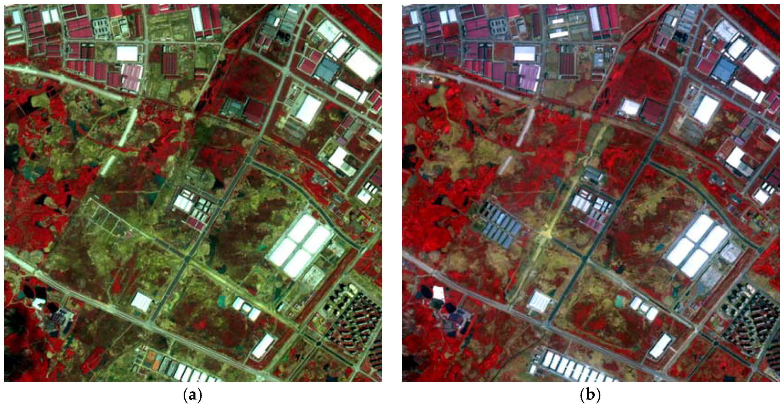
The first experiment of change detection was carried out based on a pair of GaoFen-2 (GF-2) multispectral images, as shown in Figure 2. The multispectral images contained three visible spectral bands and one near-infrared band. The image size was $3000\times 3000$, with the resolution of 4 m. Accurate coregistration was employed with ground control points (GCPs), and the residual mis-registration was less than 1 pixel. The study scene covered the Hanyang urban area of Wuhan city, Hubei province, China. Due to the rapid development of Wuhan, the study area showed obvious land-cover changes.

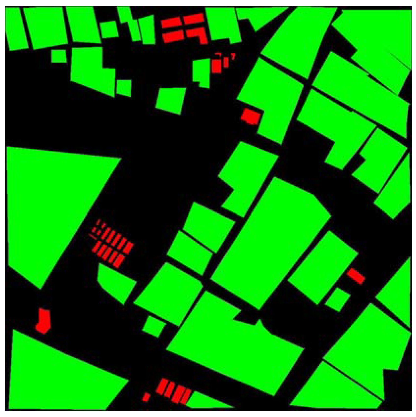
The reference map was selected by manual interpretation, which is shown in Figure 3. The changed pixels are labeled as red with the number of 106,851, and the unchanged pixels are shown as labeled with the number of 1,269,986. The change detection was regarded as a two-class classification problem, where change and nonchange were the two classes. Then, with the selected change and nonchange samples, the confusion matrix for a two-class classification could be generated, and the evaluation values, including Kappa, overall accuracy (OA), detection rate (DR), false alarm rate (FAR), and F1-Score, were calculated.

In the GF-2 dataset, the value range of the pixels was from 0–1000. If the pixels were overexposed, the spectral features would not follow the tendency of spectral differences caused by different observation environments at different times. These overexposed pixels would lead to pseudo changes that decreased change detection accuracy. Therefore, the pixels, the values of which were higher than 980 in both multitemporal images, were determined as overexposed and excluded from the calculation and evaluation. Besides, since the unchanged water areas in the image showed quite different spectral features, the water areas were also excluded from the calculation and evaluation by thresholding the NDWI features. The NDWI features of the multitemporal images were calculated separately, and 0.35 was used as a threshold to extract water areas in both images. The areas belonging to water in both images were masked.

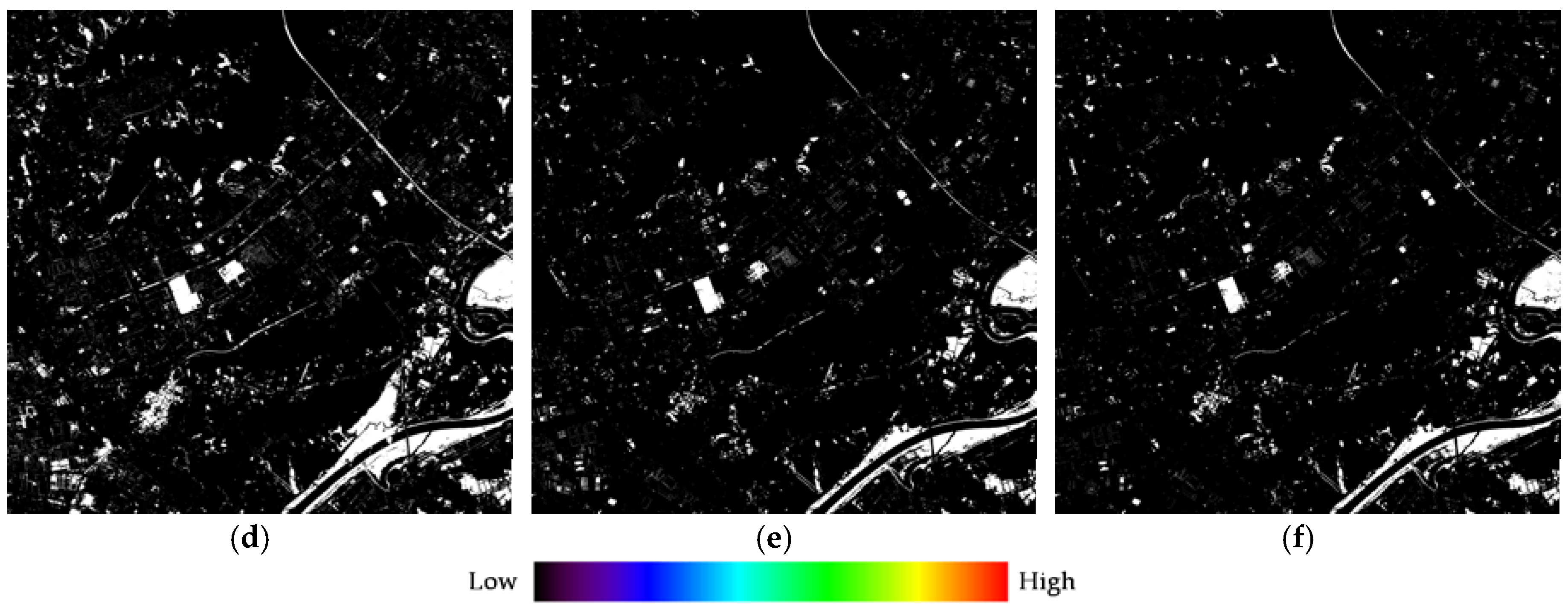
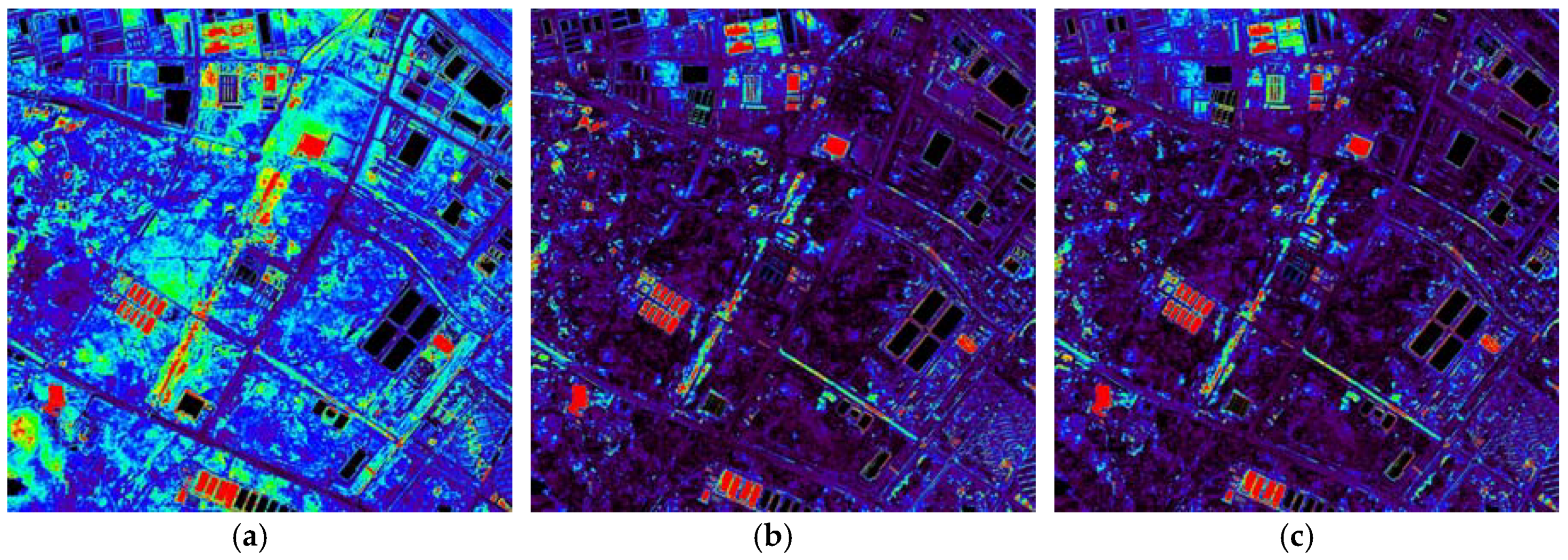
The change intensity of CVA, IRMAD, and ISFA are shown in Figure 4a–c. After the OTSU automatic thresholding, the binary change maps are shown in Figure 4d–f, where white indicates change. It can be observed that CVA, IRMAD, and ISFA detected most obvious changes. The Kappa coefficients for the binary results of CVA, IRMAD, and ISFA were 0.8444, 0.8680, and 0.8656, respectively.

In order to evaluate the performances of different thresholding methods, the quantitative assessments are shown in

Table 1. Quantitative evaluation of different thresholding methods in test dataset 1.

		Kappa	OA	DR	FAR	F1-Score
CVA	K-means	0.8444	0.9757	0.9311	0.2051	0.8576
	EM	0.7863	0.9640	0.9502	0.3007	0.8057
	OTSU	0.8444	0.9757	0.9312	0.2051	0.8576
	Max	0.8912	0.9846	0.8788	0.0786	0.8996
IRMAD	K-means	0.8666	0.9814	0.8396	0.0829	0.8766
	EM	0.5179	0.8837	0.9872	0.5976	0.5718
	OTSU	0.8680	0.9814	0.8504	0.0925	0.8780
	Max	0.8681	0.9815	0.8489	0.0906	0.8781
ISFA	K-means	0.8615	0.9814	0.8044	0.0491	0.8715
	EM	0.6109	0.9174	0.9833	0.5126	0.6518
	OTSU	0.8656	0.9818	0.8129	0.0517	0.8754
	Max	0.8884	0.9841	0.8831	0.0885	0.8970

. For quantitative assessment, Kappa coefficient and OA were used as comprehensive indicators, where the Kappa coefficient was more reliable due to the imbalance between changed reference samples and unchanged reference samples. “DR” and “FAR” were the mean detection rate and false alarm rate, respectively, while “F1-Score” was a comprehensive evaluation used in the detection problem of computer vision [48]. The best accuracies for indicators are highlighted in bold. It can be seen that, among the three automatic thresholding methods, OTSU obtained the highest accuracies, which were very close to the maximum accuracies. For the purpose of making the proposed adaptation, the binary results by OTSU automatic thresholding method were selected for the fusion of D–S theory. Combining Figure 4 and Table 1, it can be observed that CVA with OTSU can obtain a higher detection rate, while IRMAD and ISFA with OTSU can obtain a lower false alarm rate. This indicates that these three binary candidate maps can offer different information for change detection, while CVA provides more information for detecting changes, and IRMAD and ISFA provide more information for avoiding false alarms.

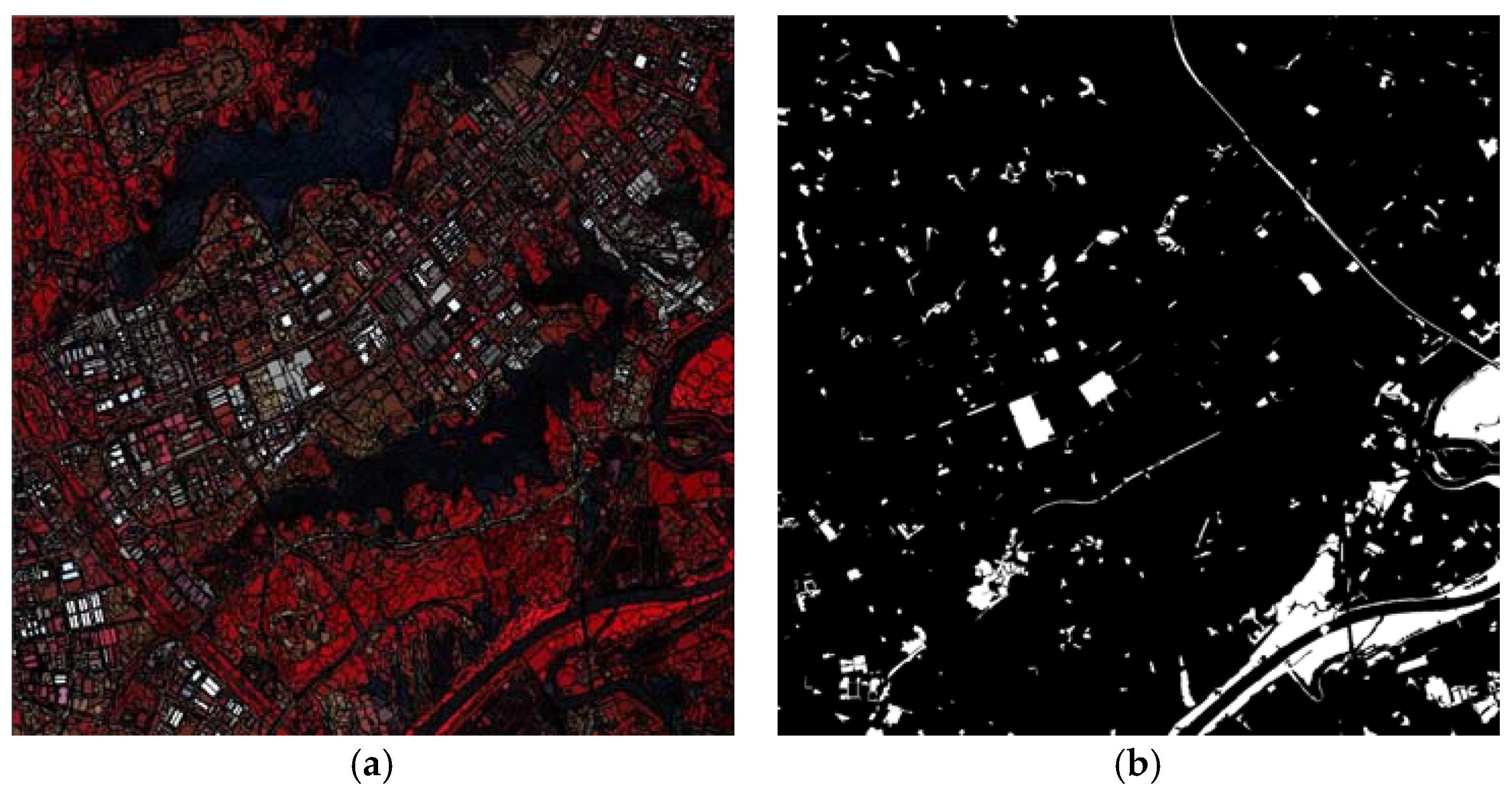
The segmentation object map is shown in Figure 5a, with the scale of 50, the shape weight of 0.5, and the compactness weight of 0.3. With this object map, the final binary change map by D–S fusion is shown in Figure 5b, where the weight $p$ for CVA, IRMAD, and ISFA are 0.7, 0.1, and 0.1, respectively.

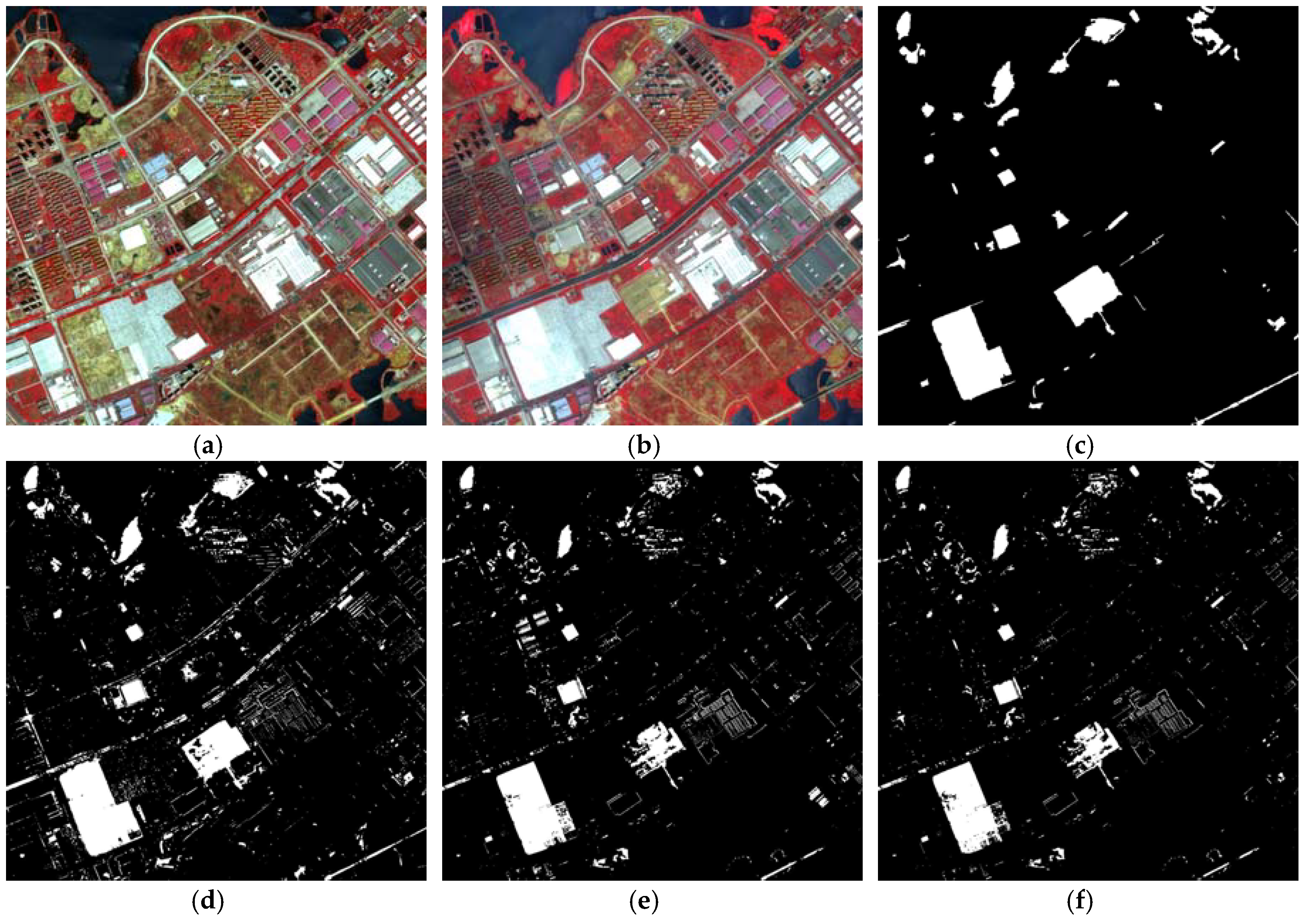
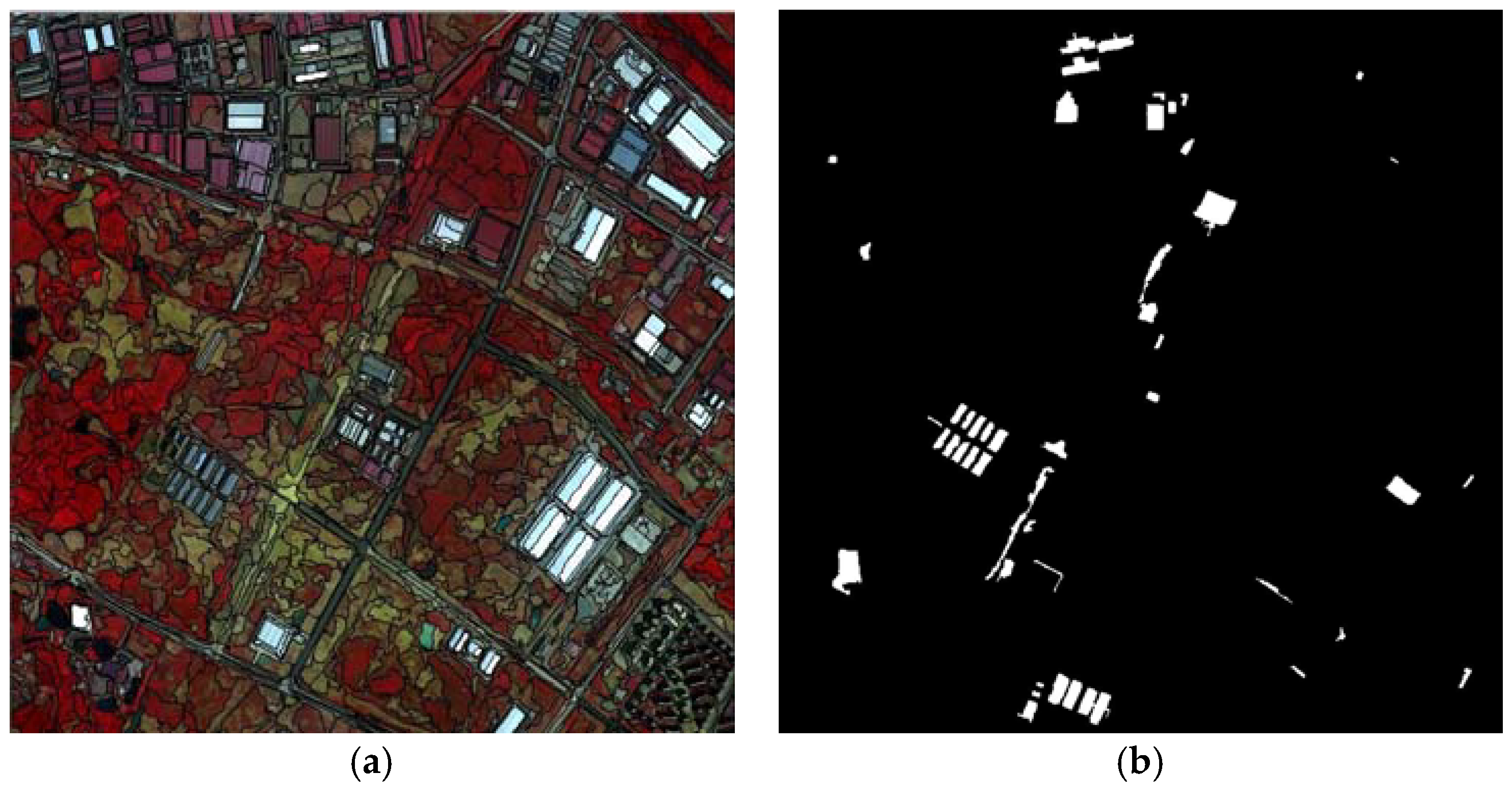
Since the study region was very large, for a better visual comparison, the zoomed multispectral images and binary change maps are shown in Figure 6. Compared with the pixelwise results, the changed objects were more complete, and most false alarms were avoided in results of the proposed method in Figure 6c. This result took advantage of the three change detection methods and decreased the uncertainty by D–S theory. The object map was considered in the fusion to keep the homogeneity of landscape objects.

In order to evaluate the performance of the proposed method, we chose the pixelwise methods and object-oriented methods for comparison. The comparison is shown in

Table 2. Quantitative evaluation of the proposed method and comparative methods in test dataset 1.

	Kappa	OA	DR	FAR	F1-Score
CVA	0.8444	0.9757	0.9312	0.2051	0.8576
IRMAD	0.8680	0.9814	0.8504	0.0925	0.8780
ISFA	0.8656	0.9818	0.8129	0.0517	0.8754
CVA_MajorVote	0.9165	0.9879	0.9252	0.0790	0.9231
IRMAD_MajorVote	0.9002	0.9865	0.8408	0.0146	0.9074
ISFA_MajorVote	0.8849	0.9847	0.8136	0.0103	0.8930
MajorVote_Fusion	0.9004	0.9866	0.8378	0.0098	0.9076
D–S_Fusion	0.9327	0.9904	0.9240	0.0478	0.9379

. “CVA”, “IRMAD”, and “ISFA” indicate the pixelwise change detection results shown in Figure 4. The automatic thresholding method utilized the OTSU method, since it showed the best performance among the automatic thresholding methods. “CVA_MajorVote”, “IRMAD_MajorVote”, and “ISFA_MajorVote” indicate the object-oriented results, where the pixelwise results were fused according to the segmentation object map in Figure 5a by major vote. “MajorVote_Fusion” indicates the result that are obtained by major vote between the three object-oriented results. Finally, “D–S_Fusion” denotes the result by the proposed method.

In Table 2, compared with the pixel-wise methods, the object-oriented methods show improvements in most cases. Especially for FAR, the objected-oriented methods can get obvious fewer false alarms than their pixelwise versions. It can prove that the object-oriented process has the ability to avoid the “salt and pepper” noise in change detection results. The “MajorVote_Fusion” by fusing the three object-oriented results did not show a better performance than its components, which is because the uncertainty between different results will negatively affect the fusion. Among all the results, the proposed method obtained the largest Kappa coefficient and overall accuracy. It showed the third largest detection rate with the fourth lowest false alarm rate, thus obtaining the largest F1-score. Therefore, Table 2 illustrates the effectiveness of the proposed fusion method.

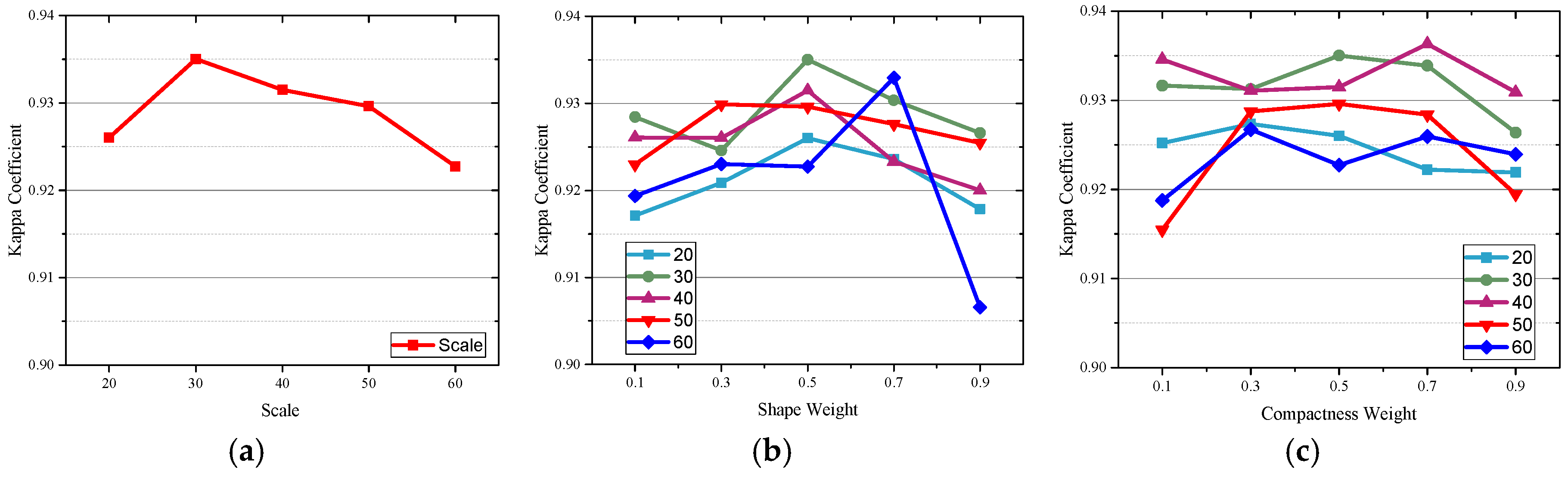
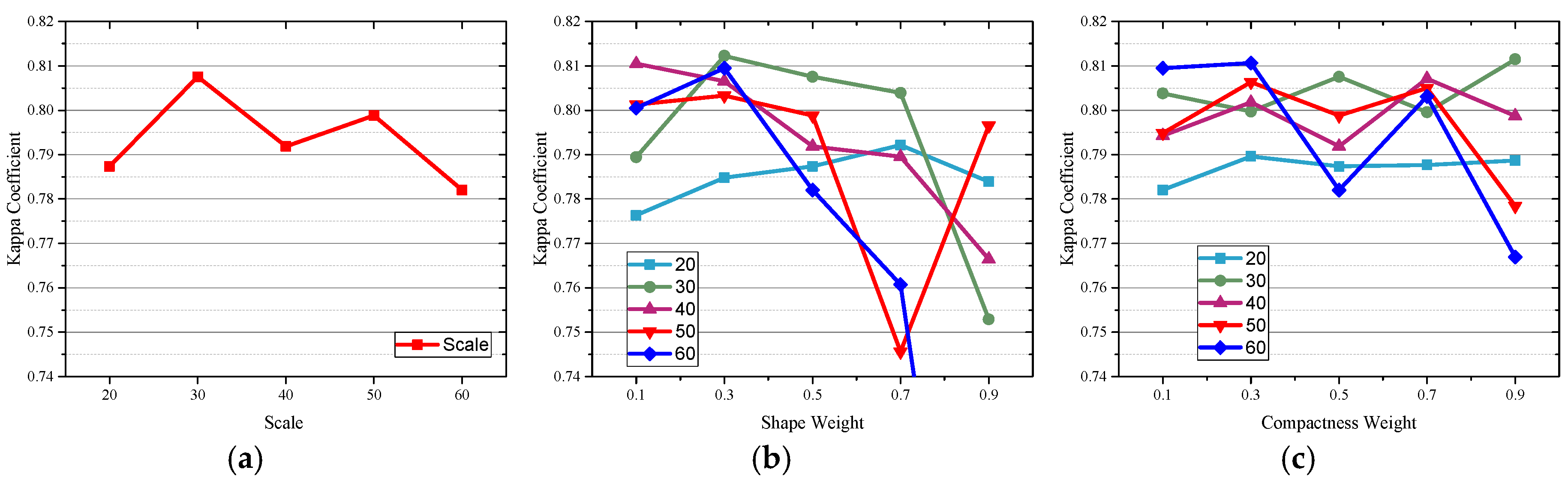
The results with different segmentation parameter settings are evaluated in Figure 7. During the evaluation, the weight $p$ in D–S fusion were fixed to be 0.9, 0.5, and 0.5. The results with different scales are evaluated in Figure 7a, when the compactness weight and shape weight are fixed to be 0.5. Figure 7a illustrates that the scale of 30 can obtain the best performance. Figure 7b shows the accuracies for different shape weights with different scales, when the compactness weight is fixed to be 0.5. When the scale is 60, the change of shape weight will lead to great differences. With other scales, the shape weight of 0.3 and 0.5 provide better performances. Figure 7c shows the different results with various compactness weights, when the shape weight is fixed to be 0.5. It illustrates that when the scale will affect the tendency of the performances. When the scale is 30 or 40, the curves are all above the others. It is worth noting that in almost all the cases, the accuracies of the proposed method are higher than 0.91, which outperforms the other methods.

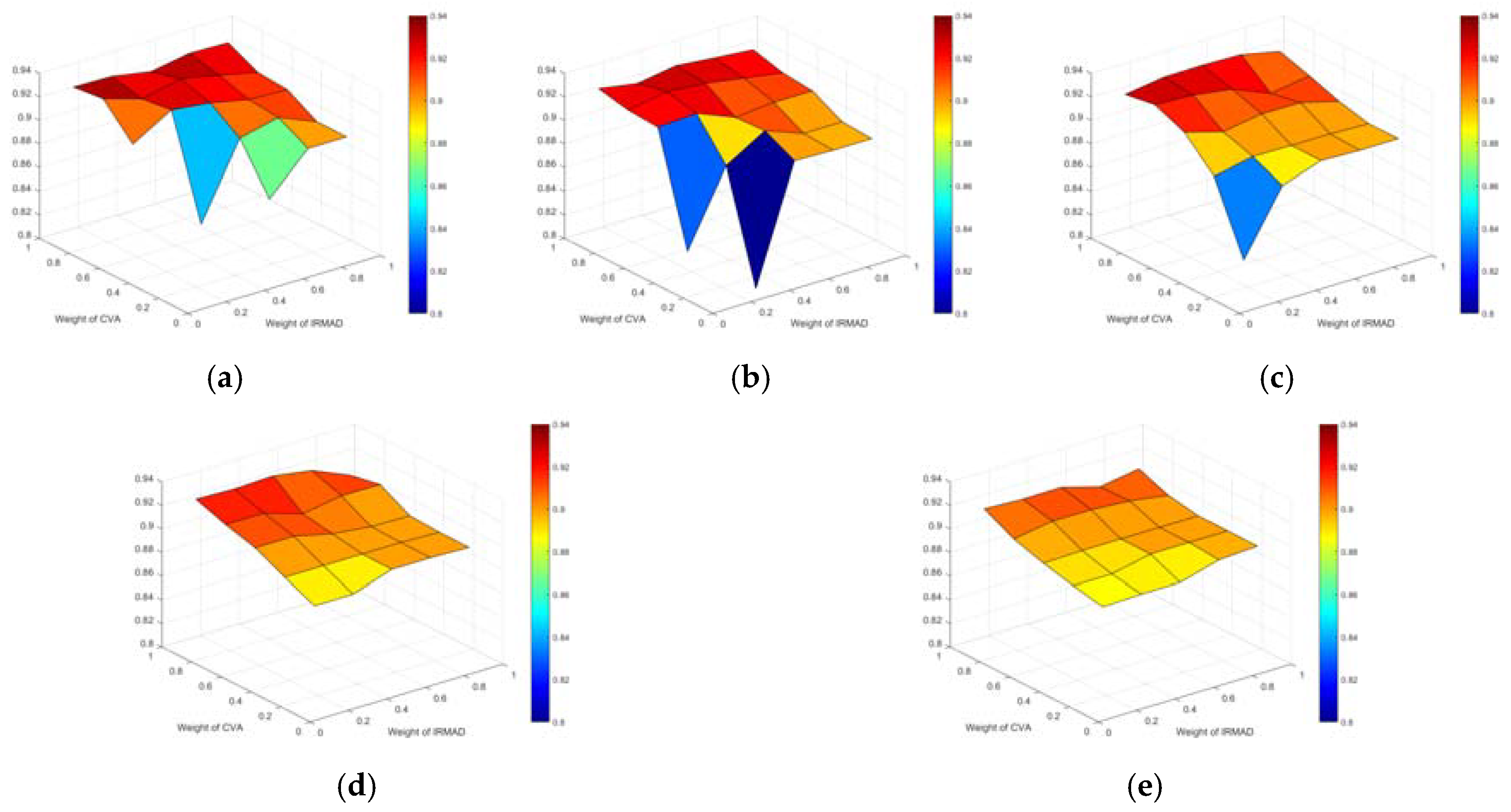
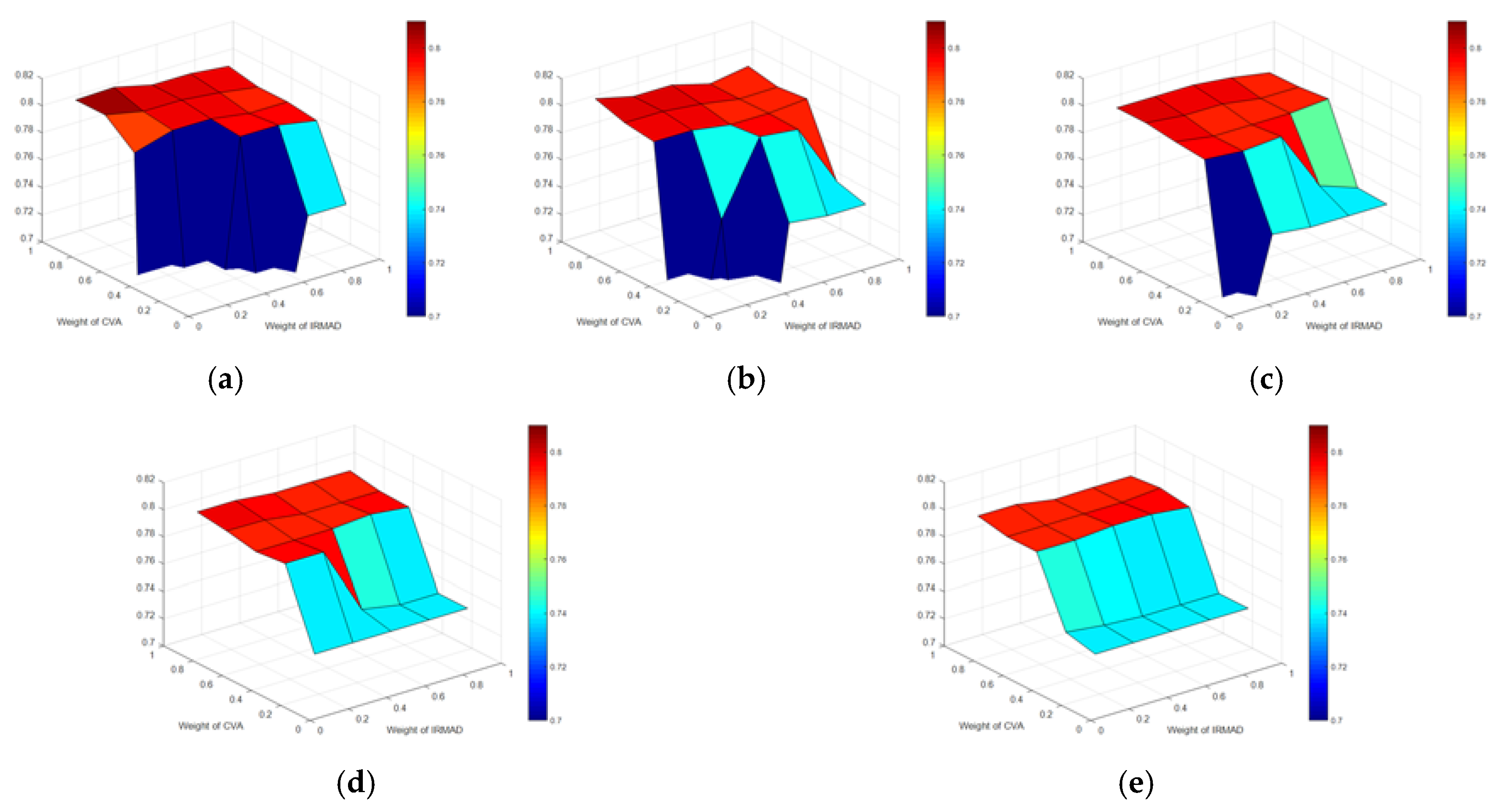
Figure 8 shows the performances with different certainty weights $p$, when the segmentation is employed with the scale of 50, the shape weight of 0.5, and the compactness weight of 0.3. The three certainty weights involved in the D–S fusion were tested with traversal combinations from 0.1 to 0.9 by step of 0.2. The Kappa coefficient surface in Figure 8 shows the Kappa values generated by a certain weight $p$ of ISFA with all the possible combinations of the other two weights. It can be observed that with the increase of $p$ for CVA, the accuracy increases obviously. Therefore, the results of CVA plays an important role in the fusion. High weight of IRMAD can also lead to good performance when the weight of CVA is very high. The increase of $p$ for ISFA leads to more robust performance.

3.2. Second Dataset

The second experiment dataset was also acquired by GF-2 with the resolution of 4 m. The study scene covered the Hanyang area of Wuhan city. The multitemporal images with the size of $1000\times 1000$ are shown in Figure 9.

The reference map of this study area is shown in Figure 10. The changed samples contained 15,975 pixels and the unchanged samples contained 484,546 pixels. The multitemporal images were preprocessed by the same approach as the first dataset. The water areas and overexposure areas were also masked from the calculation and evaluation.

The change intensity of CVA, IRMAD, and ISFA are shown in Figure 11a–c, and the binary candidate change maps with OTSU automatic thresholding are shown in Figure 11d–f. It illustrates that CVA detected more changed areas, while IRMAD and ISFA showed less false alarms. The quantitative assessment also verified this phenomenon. The detection rate for CVA was 0.7655, and comparatively, those for IRMAD and ISFA were 0.5902 and 0.6007. The false alarm rates for CVA, IRMAD, and ISFA were 0.2654, 0.1809, and 0.1959, respectively.

Table 3. Quantitative evaluation of different thresholding methods in test dataset 2.

		Kappa	OA	DR	FAR	F1-Score
CVA	K-means	0.3474	0.8964	0.9433	0.7599	0.3828
	EM	0.6869	0.9760	0.8179	0.3895	0.6991
	OTSU	0.7485	0.9833	0.7655	0.2510	0.7572
	Max	0.7687	0.9862	0.7017	0.1327	0.7758
IRMAD	K-means	0.6933	0.9781	0.7682	0.3492	0.7046
	EM	0.3943	0.9108	0.9741	0.7270	0.4265
	OTSU	0.6796	0.9818	0.5902	0.1736	0.6887
	Max	0.7018	0.9808	0.6959	0.2717	0.7117
ISFA	K-means	0.6950	0.9779	0.7810	0.3551	0.7064
	EM	0.3745	0.9036	0.9766	0.7420	0.4082
	OTSU	0.6811	0.9816	0.6007	0.1886	0.6903
	Max	0.7017	0.9813	0.6748	0.2480	0.7113

shows the quantitative evaluation of different thresholding methods. The “Max” indicates the threshold corresponding to the maximum Kappa coefficient. It can be observed that OTSU can obtain the highest Kappa coefficient for CVA, and the second highest Kappa coefficients for IRMAD and ISFA. Especially, for IRMAD and ISFA, OTSU shows the highest OA. It worth noting that OTSU can obtain good performances for all methods, while K-means show extremely low accuracy for CVA. Therefore, in order to make the proposed method automatic and robust, OTSU was selected as the automatic thresholding method to produce the binary candidate change map.

Figure 12a shows the segmentation object map, with the scale of 50, the shape weight of 0.5, and the compactness weight of 0.3. With this object map, Figure 12b shows the final binary change map by D–S fusion, where the weight $p$ for CVA, IRMAD and ISFA are 0.9, 0.1, and 0.3, respectively. Compared with the binary candidate change maps in Figure 11d–f, the fused change map shows more complete detected areas and most false alarms were removed.

Table 4. Quantitative evaluation of the proposed method and comparative methods in test dataset 2.

	Kappa	OA	DR	FAR	F1-Score
CVA	0.7485	0.9833	0.7655	0.2510	0.7572
IRMAD	0.6796	0.9818	0.5902	0.1736	0.6887
ISFA	0.6811	0.9816	0.6007	0.1886	0.6903
CVA_MajorVote	0.8018	0.9885	0.7091	0.0619	0.8077
IRMAD_MajorVote	0.7392	0.9861	0.6007	0.0161	0.7460
ISFA_MajorVote	0.7392	0.9861	0.6007	0.0161	0.7460
MajorVote_Fusion	0.7392	0.9861	0.6007	0.0161	0.7460
D–S_Fusion	0.8064	0.9888	0.7091	0.0501	0.8120

shows the quantitative evaluation of the proposed method. It illustrates that the proposed method can obtain the best accuracy with Kappa, OA, and F1-Score. The proposed method can obtain the second highest detection rate and the second lowest false alarm rate at the same time. Therefore, it shows the best performance in comprehensive evaluators. All the results with major vote got better performances than their original results, which indicates the effectiveness of the object-oriented process. However, it is worth noting that the major vote fusion with three methods cannot obtain an accurate result, since the uncertainty of each result is not taken into consideration.

Figure 13 illustrates the evaluation of segmentation parameters. The weights for CVA, IRMAD, and ISFA are fixed to be 0.9, 0.1, and 0.3. It can be found that the scale of 30 is more suitable for this dataset in Figure 13a. Figure 13b indicates that when the scale is large and the shape weight increases, the accuracy will be decreased. In Figure 13c, when the scale is 30, the accuracy with various compactness weights will be higher and more stable.

Figure 14 shows the accuracies with various weights for CVA, IRMAD, and ISFA. The parameter settings for segmentation are fixed as: the scale is 50, the shape weight is 0.5, and the compactness weight is 0.3. Figure 14 illustrates that the weight of CVA plays a key role in the fusion, since the high accuracies are mostly obtained with high weights of CVA.

4. Discussion

Since VHR multitemporal images show obvious variability within objects, it is hard to obtain a good performance by a single change detection method. When fusing different change detection results, the uncertainty is the main problem. Often, two types of uncertainty are associated with the change detection problem: one is due to the inaccuracy in each change detection result, and the other is due to the conflict between different results [41]. In the proposed method, the inaccuracy is measured by the weight of $p$ in (9). The conflict is solved by calculating the BPAF in (8). D–S evidence theory utilizes the basic probability assignment function to combine the probability of each evidence and reduce the uncertainty.

The binary change maps for different methods can be obtained by thresholding the change intensities. In order to make the proposed method adaptive, automatic thresholding methods were employed. In Table 1 and Table 3, K-means method, EM method, and OTSU method are evaluated for three change intensities and compared with the maximum accuracies. It can be found that the OTSU method outperformed the other two automatic thresholding methods in most cases and was comparatively robust. Therefore, the binary change maps by OTSU method were used for the candidate maps in the proposed D–S fusion.

The performance of the proposed method is evaluated in Table 2 and Table 4. For each component change detection result, the corresponding object-oriented results show more accurate and complete change maps. It illustrates that the object-oriented process is an effective approach to deal with multitemporal VHR imagery analysis. Table 2 and Table 4 also illustrates that the proposed method outperforms its component results (CVA, IRMAD, and ISFA). Even compared with the object-oriented fusion, the proposed D–S fusion shows higher accuracies in most cases.

According to the proposed method, the component methods with higher accuracy should be assigned as a larger $p$, since $p$ is measured as the opposite of uncertainty. As shown in Figure 7, most performances of the proposed method with the weight for CVA, IRMAD, and ISFA are 0.9, 0.5, and 0.5 are higher than the comparative methods. It can be seen in Figure 8 that with the high weight of ISFA, the proposed method can obtain good performance, which is mostly higher than 0.92. Figure 8 indicates that the high weight of ISFA can lead to more robust performance, and the result of CVA plays an important role in the D–S fusion. The accuracies of most results in Figure 8 are higher than 0.9, which are much higher than those of the candidate change maps. It indicates that the proposed method is also robust to various parameter settings. In practical applications, CVA, IRMAD, and ISFA may be more effective in different datasets [23,24,48]. The determination of weights is one of the important works in the proposed method. Figure 13 and Figure 14 also show the similar phenomena.

The main limitation of the proposed method is the parameter setting. There are two groups of parameters in the experiment. The first one is the group of segmentation parameters. The optimum setting of these parameters is affected by the resolution, object scale, and landscape distribution. Figure 7 and Figure 13 indicate that when the weights of D–S fusion are suitable, most parameter settings can lead to a better performance than the simple major vote fusion. The second group includes the weight $p$ for different evidences. Since the weight $p$ measures the uncertainty of each evidence, in most cases, the more accurate component methods should be associated with a larger $p$. However, according to the experiments, the determinations of weights are not independent, and there are interactions among different weights. It can be observed that CVA shows higher detection rate, while IRMAD and ISFA show lower false alarms. Therefore, CVA provides more information about changed areas, and IRMAD and ISFA play a part in avoiding false alarms. Accordingly, the result of CVA is assigned as high weights to better detect changes, and one of the results of IRMAD and ISFA is assigned with comparatively low weights to provide complementary information.

It is hard to determine the weight $p$ automatically. For this problem, we can introduce several effective ways. Firstly, the weight $p$ can be determined according to interpretation and expert knowledge. With the interpretation of the binary candidate change map, the weight $p$ can be estimated manually. Secondly, the weight $p$ can be evaluated according to experiment in a smaller classical study area. Some statistical theories, such as orthogonal experiment design (OED), can be utilized to evaluate the sensitivity of each parameter and the interaction effects among all the parameters [52,53]. Also, the best parameter setting can be estimated by OED and used for the whole experimental dataset.

5. Conclusions

Multitemporal VHR remote sensing images have shown great potentials in the applications of change detection. However, due to the spectral variability within landscape objects, it is hard to obtain an accurate result with a single method. When fusing multiple change detection results, the uncertainty between different evidences will be a big problem. Therefore, in this paper, we have proposed a novel change detection method by fusing multiple change detection results with D–S evidence theory. CVA, IRMAD, and ISFA with OTSU thresholding are the component methods providing candidate binary change maps that are regarded as the evidences. The BPAF for each evidence is calculated with the candidate change map, segmentation objects, and the weight for uncertainty. Finally, the decision for each object to be changed is made by fusing these three evidences with D–S theory.

The experiments with two VHR datasets were undertaken for evaluation. The results indicate that the proposed method can provide a more accurate change detection result. It shows the best performances in comprehensive indicators. The parameter setting for segmentation is determined according to the dataset. The weights of $p$ are related to the uncertainties of their corresponding evidence and are also affected by the correlations among different evidences.

In our future work, we will mainly focus on the parameter setting, especially on the automatic determination of weights $p$. Their optimum values and interaction effects between different evidences should be considered and analyzed. The statistical method, such as orthogonal experimental design, will be utilized for further analysis [53].

References

- Zhang, L.; Zhang, L.; Du, B. Deep learning for remote sensing data: A technical tutorial on the state of the art. IEEE Geosci. Remote Sens. Mag. 2016, 4, 22–40. [Google Scholar] [CrossRef]
- Wang, Q.; Zhang, F.; Li, X. Optimal clustering framework for hyperspectral band selection. IEEE Trans. Geosci. Remote Sens. 2018, 1–13. [Google Scholar] [CrossRef]
- Wang, Q.; Meng, Z.; Li, X. Locality adaptive discriminant analysis for spectral-spatial classification of hyperspectral images. IEEE Geosci. Remote Sens. Lett. 2017, 14, 2077–2081. [Google Scholar] [CrossRef]
- Fan, C.; Wang, L.; Liu, P.; Lu, K.; Liu, D. Compressed sensing based remote sensing image reconstruction via employing similarities of reference images. Multimed. Tools Appl. 2016, 75, 12201–12225. [Google Scholar] [CrossRef]
- Wang, L.; Zhang, J.; Liu, P.; Choo, K.-K.R.; Huang, F. Spectral–spatial multi-feature-based deep learning for hyperspectral remote sensing image classification. Soft Comput. 2017, 21, 213–221. [Google Scholar] [CrossRef]
- Dou, M.; Chen, J.; Chen, D.; Chen, X.; Deng, Z.; Zhang, X.; Xu, K.; Wang, J. Modeling and simulation for natural disaster contingency planning driven by high-resolution remote sensing images. Future Gener. Comput. Syst. 2014, 37, 367–377. [Google Scholar] [CrossRef]
- Lu, D.; Mausel, P.; Brondizio, E.; Moran, E. Change detection techniques. Int. J. Remote Sens. 2004, 25, 2365–2401. [Google Scholar] [CrossRef]
- Coppin, P.; Jonckheere, I.; Nackaerts, K.; Muys, B.; Lambin, E. Digital change detection methods in ecosystem monitoring: A review. Int. J. Remote Sens. 2004, 25, 1565–1596. [Google Scholar] [CrossRef]
- Singh, A. Review article digital change detection techniques using remotely-sensed data. Int. J. Remote Sens. 1989, 10, 989–1003. [Google Scholar] [CrossRef]
- Zhang, J.; Zhang, Y. Remote sensing research issues of the national land use change program of china. ISPRS J. Photogramm. 2007, 62, 461–472. [Google Scholar] [CrossRef]
- Kennedy, R.E.; Townsend, P.A.; Gross, J.E.; Cohen, W.B.; Bolstad, P.; Wang, Y.Q.; Adams, P. Remote sensing change detection tools for natural resource managers: Understanding concepts and tradeoffs in the design of landscape monitoring projects. Remote Sens. Environ. 2009, 113, 1382–1396. [Google Scholar] [CrossRef]
- Li, H.; Xiao, P.; Feng, X.; Yang, Y.; Wang, L.; Zhang, W.; Wang, X.; Feng, W.; Chang, X. Using land long-term data records to map land cover changes in china over 1981–2010. IEEE J. Sel. Top. Appl. Earth Obs. Remote Sens. 2017, 10, 1372–1389. [Google Scholar] [CrossRef]
- Li, Z.; Shi, W.; Myint, S.W.; Lu, P.; Wang, Q. Semi-automated landslide inventory mapping from bitemporal aerial photographs using change detection and level set method. Remote Sens. Environ. 2016, 175, 215–230. [Google Scholar] [CrossRef]
- Song, C.; Huang, B.; Ke, L.; Richards, K.S. Remote sensing of alpine lake water environment changes on the tibetan plateau and surroundings: A review. ISPRS J. Photogramm. 2014, 92, 26–37. [Google Scholar] [CrossRef]
- Xian, G.; Homer, C.; Fry, J. Updating the 2001 national land cover database land cover classification to 2006 by using landsat imagery change detection methods. Remote Sens. Environ. 2009, 113, 1133–1147. [Google Scholar] [CrossRef]
- Vittek, M.; Brink, A.; Donnay, F.; Simonetti, D.; Desclée, B. Land cover change monitoring using landsat mss/tm satellite image data over west africa between 1975 and 1990. Remote Sens. 2014, 6, 658–676. [Google Scholar] [CrossRef] [Green Version]
- Araya, Y.H.; Cabral, P. Analysis and modeling of urban land cover change in setúbal and sesimbra, portugal. Remote Sens. 2010, 2, 1549–1563. [Google Scholar] [CrossRef]
- Rokni, K.; Ahmad, A.; Selamat, A.; Hazini, S. Water feature extraction and change detection using multitemporal landsat imagery. Remote Sens. 2014, 6, 4173–4189. [Google Scholar] [CrossRef]
- Hussain, M.; Chen, D.; Cheng, A.; Wei, H.; Stanley, D. Change detection from remotely sensed images: From pixel-based to object-based approaches. ISPRS J. Photogramm. 2013, 80, 91–106. [Google Scholar] [CrossRef]
- Bovolo, F.; Bruzzone, L. A theoretical framework for unsupervised change detection based on change vector analysis in the polar domain. IEEE Trans. Geosci. Remote Sens. 2007, 45, 218–236. [Google Scholar] [CrossRef]
- Ridd, M.K.; Liu, J. A comparison of four algorithms for change detection in an urban environment. Remote Sens. Environ. 1998, 63, 95–100. [Google Scholar] [CrossRef]
- Carvalho Júnior, O.A.; Guimarães, R.F.; Gillespie, A.R.; Silva, N.C.; Gomes, R.A.T. A new approach to change vector analysis using distance and similarity measures. Remote Sens. 2011, 3, 2473–2493. [Google Scholar] [CrossRef]
- Wu, C.; Du, B.; Zhang, L. Slow feature analysis for change detection in multispectral imagery. IEEE Trans. Geosci. Remote Sens. 2014, 52, 2858–2874. [Google Scholar] [CrossRef]
- Nielsen, A.A. The regularized iteratively reweighted mad method for change detection in multi- and hyperspectral data. IEEE Trans. Image Process. 2007, 16, 463–478. [Google Scholar] [CrossRef] [PubMed]
- Celik, T. Unsupervised change detection in satellite images using principal component analysis and k-means clustering. IEEE Geosci. Remote Sens. Lett. 2009, 6, 772–776. [Google Scholar] [CrossRef]
- Huang, Z.; Jia, X.P.; Ge, L.L. Sampling approaches for one-pass land-use/land-cover change mapping. Int. J. Remote Sens. 2010, 31, 1543–1554. [Google Scholar] [CrossRef]
- Yuan, F.; Sawaya, K.E.; Loeffelholz, B.C.; Bauer, M.E. Land cover classification and change analysis of the twin cities (minnesota) metropolitan area by multitemporal landsat remote sensing. Remote Sens. Environ. 2005, 98, 317–328. [Google Scholar] [CrossRef]
- Lei, Z.; Fang, T.; Huo, H.; Li, D. Bi-temporal texton forest for land cover transition detection on remotely sensed imagery. IEEE Trans. Geosci. Remote Sens. 2014, 52, 1227–1237. [Google Scholar] [CrossRef]
- Huang, X.; Zhu, T.; Zhang, L.; Tang, Y. A novel building change index for automatic building change detection from high-resolution remote sensing imagery. Remote Sens. Lett. 2014, 5, 713–722. [Google Scholar] [CrossRef]
- Bruzzone, L.; Bovolo, F. A novel framework for the design of change-detection systems for very-high-resolution remote sensing images. Proc. IEEE 2013, 101, 609–630. [Google Scholar] [CrossRef]
- Brunner, D.; Lemoine, G.; Bruzzone, L. Earthquake damage assessment of buildings using vhr optical and sar imagery. IEEE Trans. Geosci. Remote Sens. 2010, 48, 2403–2420. [Google Scholar] [CrossRef]
- Tang, Y.; Zhang, L. Urban change analysis with multi-sensor multispectral imagery. Remote Sens. 2017, 9, 252. [Google Scholar] [CrossRef]
- Sun, L.; Tang, Y.; Zhang, L. Rural building detection in high-resolution imagery based on a two-stage cnn model. IEEE Geosci. Remote Sens. Lett. 2017, 14, 1998–2002. [Google Scholar] [CrossRef]
- Volpi, M.; Tuia, D.; Bovolo, F.; Kanevski, M.; Bruzzone, L. Supervised change detection in vhr images using contextual information and support vector machines. Int. J. Appl. Earth Obs. Geoinf. 2013, 20, 77–85. [Google Scholar] [CrossRef]
- Wang, Q.; Wan, J.; Yuan, Y. Locality constraint distance metric learning for traffic congestion detection. Pattern Recognit. 2018, 75, 272–281. [Google Scholar] [CrossRef]
- Wang, Q.; Gao, J.; Yuan, Y. A joint convolutional neural networks and context transfer for street scenes labeling. IEEE Trans. Intell. Transp. Syst. 2018, 19, 1457–1470. [Google Scholar] [CrossRef]
- Tang, Y.; Zhang, L.; Huang, X. Object-oriented change detection based on the kolmogorov–smirnov test using high-resolution multispectral imagery. Int. J. Remote Sens. 2011, 32, 5719–5740. [Google Scholar] [CrossRef]
- Ma, L.; Li, M.; Blaschke, T.; Ma, X.; Tiede, D.; Cheng, L.; Chen, Z.; Chen, D. Object-based change detection in urban areas: The effects of segmentation strategy, scale, and feature space on unsupervised methods. Remote Sens. 2016, 8, 761. [Google Scholar] [CrossRef]
- Wen, D.; Huang, X.; Zhang, L.; Benediktsson, J.A. A novel automatic change detection method for urban high-resolution remotely sensed imagery based on multiindex scene representation. IEEE Trans. Geosci. Remote Sens. 2016, 54, 609–625. [Google Scholar] [CrossRef]
- Gueguen, L.; Pesaresi, M.; Ehrlich, D.; Lu, L.; Guo, H. Urbanization detection by a region based mixed information change analysis between built-up indicators. IEEE J. Sel. Top. Appl. Earth Obs. Remote Sens. 2013, 6, 2410–2420. [Google Scholar] [CrossRef]
- Dutta, P. An uncertainty measure and fusion rule for conflict evidences of big data via dempster–shafer theory. Int. J. Image Data Fusion 2017, 1–18. [Google Scholar] [CrossRef]
- Hegarat-Mascle, S.L.; Bloch, I.; Vidal-Madjar, D. Application of dempster-shafer evidence theory to unsupervised classification in multisource remote sensing. IEEE Trans. Geosci. Remote Sens. 1997, 35, 1018–1031. [Google Scholar] [CrossRef]
- Hao, M.; Shi, W.; Zhang, H.; Wang, Q.; Deng, K. A scale-driven change detection method incorporating uncertainty analysis for remote sensing images. Remote Sens. 2016, 8, 745. [Google Scholar] [CrossRef]
- Lu, Y.H.; Trinder, J.C.; Kubik, K. Automatic building detection using the dempster-shafer algorithm. Photogramm. Eng. Remote Sens. 2006, 72, 395–403. [Google Scholar] [CrossRef]
- Desclée, B.; Bogaert, P.; Defourny, P. Forest change detection by statistical object-based method. Remote Sens. Environ. 2006, 102, 1–11. [Google Scholar] [CrossRef]
- Marpu, P.R.; Gamba, P.; Canty, M.J. Improving change detection results of ir-mad by eliminating strong changes. IEEE Geosci. Remote Sens. Lett. 2011, 8, 799–803. [Google Scholar] [CrossRef]
- Canty, M.J.; Nielsen, A.A. Automatic radiometric normalization of multitemporal satellite imagery with the iteratively re-weighted mad transformation. Remote Sens. Environ. 2008, 112, 1025–1036. [Google Scholar] [CrossRef]
- Wu, C.; Zhang, L.; Du, B. Kernel slow feature analysis for scene change detection. IEEE Trans. Geosci. Remote Sens. 2017, 55, 2367–2384. [Google Scholar] [CrossRef]
- Wu, C.; Du, B.; Cui, X.; Zhang, L. A post-classification change detection method based on iterative slow feature analysis and bayesian soft fusion. Remote Sens. Environ. 2017, 199, 241–255. [Google Scholar] [CrossRef]
- Bruzzone, L.; Prieto, D.F. Automatic analysis of the difference image for unsupervised change detection. IEEE Trans. Geosci. Remote Sens. 2000, 38, 1171–1182. [Google Scholar] [CrossRef]
- Shafer, G. Dempster-shafer theory. Encycl. Artif. Intell. 1992, 330–331. [Google Scholar]
- Luo, H.; Wang, L.; Shao, Z.; Li, D. Development of a multi-scale object-based shadow detection method for high spatial resolution image. Remote Sens. Lett. 2015, 6, 59–68. [Google Scholar] [CrossRef]
- Luo, H.; Li, D.; Liu, C. Parameter evaluation and optimization for multi-resolution segmentation in object-based shadow detection using very high resolution imagery. Geocarto Int. 2017, 32, 1307–1332. [Google Scholar] [CrossRef]
Figure 1.
Flowchart of the proposed method.
Figure 2.
The pseudocolor VHR images acquired by GF-2 satellite on (a) 11 April 2016; and (b) 1 September 2016.
Figure 3.
The reference map where red indicates change and green indicates nonchange.
Figure 4.
The change intensities with rainbow colors of (a) CVA; (b) IRMAD; (c) ISFA, and the binary change maps of (d) CVA; (e) IRMAD; (f) ISFA.
Figure 5.
(a) The segmentation object map; and (b) binary change map after D–S fusion.
Figure 6.
The zoomed multispectral images on (a) 11 April 2016; and (b) 1 September 2016; and the zoomed binary change maps of (c) the proposed method; (d) CVA; (e) IRMAD; and (f) ISFA.
Figure 7.
Parameter evaluation for (a) scale; (b) shape weight; and (c) compactness weight in test dataset 1.
Figure 8.
The quantitative evaluation with the ISFA weight of (a) 0.1; (b) 0.3; (c) 0.5; (d) 0.7; and (e) 0.9 in test dataset 1.
Figure 9.
Figure 10.
Figure 11.
The change intensity of (a) CVA; (b) IRMAD; (c) ISFA; and the binary change map of (d) CVA; (e) IRMAD; (f) ISFA.
Figure 12.
Figure 13.
Parameter evaluation for (a) scale; (b) shape weight; and (c) compactness weight in test dataset 2.
Figure 14.
The quantitative evaluation with the ISFA weight of (a) 0.1; (b) 0.3; (c) 0.5; (d) 0.7; and (e) 0.9 in test dataset 2.