Doppler Frequency Estimation of Point Targets in the Single-Channel SAR Image by Linear Least Squares


Department of Earth System Sciences, Yonsei University, Seoul 03722, Korea
Remote Sens. 2018, 10(7), 1160; https://doi.org/10.3390/rs10071160
Submission received: 14 June 2018
/
Revised: 12 July 2018
/
Accepted: 20 July 2018
/
Published: 23 July 2018
Abstract
:This paper presents a method and results for the estimation of residual Doppler frequency, and consequently the range velocity component of point targets in single-channel synthetic aperture radar (SAR) focused single-look complex (SLC) data. It is still a challenging task to precisely retrieve the radial velocity of small and slow-moving objects, which requires an approach providing precise estimates from only a limited number of samples within a few range bins. The proposed method utilizes linear least squares, along with the estimation of signal parameters via rotational invariance techniques (ESPRIT) algorithm, to provide optimum estimates from sets of azimuth subsamples that have different azimuth temporal distances. The ratio of estimated Doppler frequency to root-mean square error (RMSE) is suggested for determining a critical threshold, optimally selecting a number of azimuth subsample sets to be involved in the estimation. The proposed method was applied to TerraSAR-X and KOMPSAT-5 X-band SAR SLC data for on-land and coastal sea estimation, with speed-controlled, truck-mounted corner reflectors and ships, respectively. The results demonstrate its performance of the method, with percent errors of less than 5%, in retrieved range velocity for both on-land and in the sea. It is also robust, even for weak targets with low peak-to-sidelobe ratios (PSLRs) and signal-to-clutter ratios (RCSs). Since the characteristics of targets and clutter on land and in the sea are different, it is recommended that the method is applied separately with different thresholds. The limitations of the approach are also discussed.
1. Introduction
Some multi-channel synthetic aperture radar (SAR) systems and techniques have been developed specifically for detection and velocity retrieval of ground moving target indication (GMTI), such as along-track interferometric (ATI) systems [1,2,3,4,5,6,7]. Or, displaced phase center antenna (DPCA) systems [8,9,10,11,12], and raw data-based methods such as space-time adaptive processing (STAP) [13,14,15]. However, SAR data availability recorded by these multi-channel systems is so far very limited compared with single-channel SAR data [16]. Currently, various space-borne single-channel SAR systems are available, but it is still challenging to utilize them for detection and velocity retrieval of ground moving targets. The performance of single-channel SAR estimates on the ground moving target is useful, but not comparable with that of the ATI SAR systems, in terms of the measurement accuracy [17]. One can classify ground moving objects into two groups: one consists of ground motion in groups such as ocean currents and waves, and the other entails isolated small moving objects that are considered as individual point targets, for instance moving boats or cars. While it is possible to adopt a statistical approach for the former case, it is necessary for the latter to estimate Doppler parameters from a single, or at most a few, range bins of SAR signals. Both along-track and range components of object movement changes the Doppler history in comparison to the clutter [8,18,19,20]. A target motion in the range direction modifies a Doppler frequency, which results in an azimuth displacement of the object in the normally focused image, due to the shift of the Doppler frequency [8]. The along-track velocity component affects a Doppler frequency rate, resulting in a blurring of the normally focused image [8]. Thus, a precise estimation of the Doppler parameters is the key to the detection and velocity retrieval of ground moving targets by single-channel SAR observation. An efficient residual focusing is also possible once the two velocity components are obtained [21]. The main goal of this paper is to propose a high-performance method for accurate estimation of the residual Doppler frequency and consequently, the range velocity component of the point targets from the single-channel SAR focused single-look complex (SLC) data. The estimation of Doppler frequency rate or the azimuth velocity component is beyond the scope of this paper. The residual Doppler frequency in this paper is defined as a Doppler frequency of a point target residing in the SLC data normally associated with the motion of the target, while the Doppler centroid represents the averaged Doppler frequency of stationary ground objects, required mainly for SAR focusing in relation to the antenna look and squint angles. A number of methods have been proposed for GMTI, since the characteristics of SAR returned signals were discussed by [8], and most of them are based on sensing the difference in Doppler parameters between the moving object and the stationary clutter. A simple method of Doppler parameter estimation based on Doppler frequency shifts was proposed by [22]. A Doppler filtering method, which requires a pulse repetition frequency (PRF) four times larger than the clutter bandwidth, was proposed by [23]. Joint time-frequency analysis (JTFA) has been popularly used to measure the object motion directly from SAR raw signals, and it has demonstrated the potential to extract a time sequence of motion parameters [24,25]. It was shown that the time-frequency signature of a moving object is significantly different from the signatures of a stationary object, even when the SAR images of the two are similar [26]. It must be noted that most GMTI methods utilize SAR raw signals, rather than the focused SLC data. However, it is emphasized that it is not practical for most users to process raw signals, because the raw signal data acquired by most current high-resolution SAR systems are simply not available to general users. Thus, it is presumed in this study that only the SAR SLC data, not raw signals, are available in this study. The motivation for this study is to develop an improved residual Doppler frequency estimator specifically for small and slow-moving targets, for instance small fishing boats and vehicles, from space-borne single channel SAR SLC data. Although many sophisticated methods have been developed for GMTI, it is so far a challenging task to precisely measure the radial velocity of small and slow-moving objects from space.
For the Doppler centroid estimation, many approaches have been developed mainly for SAR image focusing. Some popularly used methods include: Energy balancing [27]; the average cross correlation coefficient method [28]; the spectral fit approach [29]; multi-look cross correlation; and the multi-look beat frequency algorithm [30]. It is shown that due to the effect of antenna pattern, reflectivity and system transfer function, the averaged Doppler power spectrum can be modelled by a sine wave on a pedestal [31]. A performance of various Doppler centroid estimation was discussed in detail by [28]. More recently, different approaches have been proposed. A method based upon the maximum likelihood estimator in the time domain was proposed by [32]. A Radon transform-based Doppler parameter estimator was proposed by [33]. Although these methods provide very reliable estimates, they are basically developed for SAR focusing and require an averaging process over a number of range bins. To measure the Doppler frequency of point targets associated with ground moving targets, the Doppler parameters must be calculated using only a few range bins. For this purpose, a method examining the skew of the received signal in the two-dimensional frequency domain was discussed by [34] to resolve the un-aliased range velocity component. The joint time-frequency analysis is also useful for this purpose, by using a mean conditional frequency (MCF) from the Wigner-Ville distribution [18,19]. The statistical model for the echo backscattered by the homogeneous ground surface can be modelled as a Gaussian function in the Wigner-Ville distribution [19,24]. Based on this property, a Doppler spectrum tracing method was proposed in joint a time-frequency domain by [35]. They concluded that their method is very useful for fast moving targets, but it is only effective if the target speed is at least 5 km/h (or 1.4 m/s) or higher. Recently, a sophisticated algorithm of Doppler centroid estimation for improving ship detection with radial velocity estimation was proposed by [36], in which the characteristics of Doppler spectrum of ships were well discussed. The method in [36] exploited the clutter-lock algorithm and demonstrated an accurate retrieval of radial velocity of ships with a root-mean-square (rms) deviation of less than 5% at ship speeds higher than or equal to 2 m/s (or 7.2 km/h).
To accommodate moving targets at low speed, this paper focuses on a precise estimation of the residual Doppler frequency occurring by point targets in single-channel SAR SLC data. The problem at hand has serious restrictions on the application of the conventional methods. Firstly, the Doppler spectrum of a point target with a low signal-to-clutter ratio (SCR) is severely distorted, and too difficult to precisely determine a residual Doppler frequency. Secondly, a point target often extends less than a few range bins, which restricts a spectral averaging over a number of range bins. Thirdly, the number of azimuth samples for the estimation should be limited to minimize the effects of phase interference by clutter. For instance, the nth zeros of the sinc function for a point target is in slow-time?which is approximately in azimuth samples?if the ratio of Doppler bandwidth () to the pulse repetition frequency (PRF) is 0.8. To account for up to 10 side-lobes, the total number of samples for the frequency estimation is no larger than 25. These facts often make the conventional spectral analysis in the Doppler frequency domain ineffective.
Other potential approaches for Doppler frequency estimation are parametric methods, such as the estimation of signal parameters via rotational invariance techniques (ESPRIT) [37,38], the multiple signal classification (MUSIC) [39], etc. The parametric methods generally offer better estimates when a number of data is limited, and the signal closely agrees with an assumed model; the ESPRIT provides more accurate estimates than the other methods among various parametric methods [40]. The ESPRIT algorithm was proposed to estimate the frequencies of a set of complex exponentials in noise, and it was further developed in the context of array signal processing [37,38]. Santamaria et al. [41] did comparative studies of various high-accuracy frequency estimation methods, and concluded that ESPRIT is good for high signal-to-noise ratios (SNRs). Despite its good statistical properties and high-resolution capability, the high computational cost of ESPRIT precludes its use in real-time frequency estimation applications (Santamaria et al., 2010). The parametric methods, however, cannot fully overcome the restrictions on the point targets imaged by the single-channel SAR system. The ESPRIT method exploits eigenvector decomposition of the sample covariance matrix and provides highly accurate estimates when SNRs are high [40]. However, the sample covariance matrix with an original azimuth sampling distance and a limited number of samples might be highly corrupted by clutter at low SCR, as well as low peak-to-sidelobe ratio (PSLR). The sample covariance is calculated by a complex conjugate multiplication of data samples with successive azimuth samples, which often results in a serious interference of the signal Doppler phase by clutter. Particularly, when they are with low PSLRs and RCSs, an original fixed sample temporal distance—for instance, 1/PRF is not good enough to provide accurate estimates. To overcome this limitation, the proposed method in this paper introduces following ideas: First, it is possible to make new sets of azimuth samples for multiplication with a different azimuth temporal distance by applying a similar technique developed for bistatic SAR digital beamforming [42]. Once the new sets of data with different azimuth temporal distance are obtained, Doppler frequency for each pair of the data is estimated by the ESPRIT. The estimates are now a time series of the estimated Doppler frequency at each corresponding azimuth temporal distance. Then, the time series of Doppler frequency estimates is solved by a normal equation of linear least squares to obtain an optimum estimate of the Doppler frequency. With this approach, the measurement accuracy of the Doppler frequency can be significantly improved even under conditions of low PSRLs and SCRs. The novelty of the proposed method lies on the facts that samples of one or a few range bins are enough to estimate Doppler parameters with a high degree of accuracy, which extends the application capability of single-channel SAR systems to small and/or slow-moving targets.
The remainder of this paper is organized as follows: In Section 2, the theoretical background of the proposed method is introduced and discussed with a pseudocode of the proposed method. Section 3 provides the results of the proposed method by applying it to the TerraSAR-X and KOMPSAT-5 single-channel X-band SAR SLC data. The former is for examples of on-land application, using vehicles—among which one is a speed controlled and truck-mounted corner reflector for the experiment and others are detected within the SAR image. The latter is for the demonstration of Doppler frequency estimation in the coastal sea. The heading and speed of a ship was precisely measured by an on-board GPS system for this experiment, and other ships were detected ones within the image. The results from the field experiments demonstrate the application capability of the proposed method, followed by a discussion about the limitations of the method and conclusions in Section 4 and Section 5, respectively.
2. Theoretical Background
2.1. Linear Least Squares for Doppler Frequency Estimation
Provided that a point target is focused with a residual Doppler frequency, , a point target in a single-look complex SAR image can be described by a simple model such as Reference [21],
where is slow-time (or azimuth time), is Doppler bandwidth, is residual Doppler frequency, and is the phase of the signal. Since here we focus on the Doppler frequency, the residual Doppler rate associated with the azimuth velocity component is neglected, without any loss of generality. A straightforward method is a spectral analysis in the frequency domain via Fourier Transform. However, the random phase noise induced by neighboring objects and other various causes is problematic and it often makes the spectral analysis difficult to precisely measure the residual Doppler frequency without averaging over a number of range bins.
Meanwhile, most parametric methods are based on the eigenvector decomposition of sample covariance matrix. The sample covariance calculation results in phase differentiation by
where is a complex conjugate operation, and are the sample interval and amplitude, respectively, and the phase term is given by
where is phase noise. The accuracy of the parametric estimate largely depends upon the signal to noise ratio. While the phase noise greatly varies according to the signal-to-clutter ratio, a small value of () makes it difficult to precisely measure, unless a point target has a large and a large signal-to-clutter ratio. The core idea of the proposed method is based on a linear least squares estimation to determine an optimal with a variable of . Instead of a fixed azimuth sample interval , consider a general linear regression model
where the parameter and are to be determined, and is the error term. If one has a set of data, such as
or equivalently
then , , , and are each a corresponding matrix in Equation (5). It is well known that the least squares method achieves a statistically optimal solution by the normal equation
where is a matrix transpose and is a matrix inverse. A computational efficiency can be improved by considering a special property of Equation (7). The inverse matrix of Equation (7) can be simplified if the second column of matrix is time symmetry, that is
where
Then, the inverse matrix is simply given by
The calculation of the second bracket in Equation (7) is also explicitly expressed by
From Equations (7), (9) and (10), the linear least squares solution is obtained by
and
Since we are interested in the Doppler frequency, it is necessary only to compute Equation (12). Equation (12) is an accumulation of phase derivative multiplied by the corresponding temporal distance, . Thus, the total size of required temporary data storage is the same as that of the image. The normal equation solution of an matrix requires a computational cost of O((2N + 1)2 × (2N + 1+ 2)). On the contrary, a total number of computational steps is O(2N + 1), and N = 3 to 5 usually is enough to obtain a good estimate. Thus, the computational efficiency is made very competitive by introducing a simple solution of a normal equation in Equation (12), instead of a matrix inversion.
2.2. Azimuth Subsamples
To estimate Doppler frequency through the linear least squares, it is necessary to have a series of signal pairs in Equation (2) with various temporal distance, . Since the monostatic SAR system receives returned signals only at every azimuth sampling interval (i.e., usually 1/PRF), it is necessary to make azimuth subsamples. One simple and effective method is to apply a point target response of a bistatic SAR, given by Reference [42],
where is the satellite velocity, the wavelength and is the distance between the transmitting and receiving antenna. Equation (13) indicates that the bistatic response is obtained from the monostatic SAR signals by a time delay, , and a phase shift by . Azimuth subsamples at any given are effectively and efficiently obtained by Equation (13), which is achieved by a simple multiplication of the monostatic SAR signals in the Doppler frequency domain. The distance can be chosen arbitrarily. For our application, the distance is used to satisfy a given fraction of azimuth sampling interval.
Processing flow of the proposed method is summarized as the pseudocode in Table 1. To estimate Doppler frequency at each over a few tens of azimuth samples, the ESPRIT algorithm was used in this study. However, it requires the highest computational cost. The ESPRIT algorithm is based upon the eigenvector decomposition of a 2 by 2 sample covariance matrix in this SAR application, and the singular-value decomposition (SVD) is the key to computational efficiency. The computation of SVD for an m × n matrix would cost O (n × m2 + m × n2 + n3). The computational efficiency can be significantly improved by replacing the SVD with an explicit solution of eigenvalue and eigenvector of the 2 by 2 covariance matrix. The computation of the explicit solution needs only simple arithmetic calculations [43], and the total number of required computations is comparable to that of convolution.
3. Application Results
3.1. SAR SLC Data Used for Evaluation and Validation
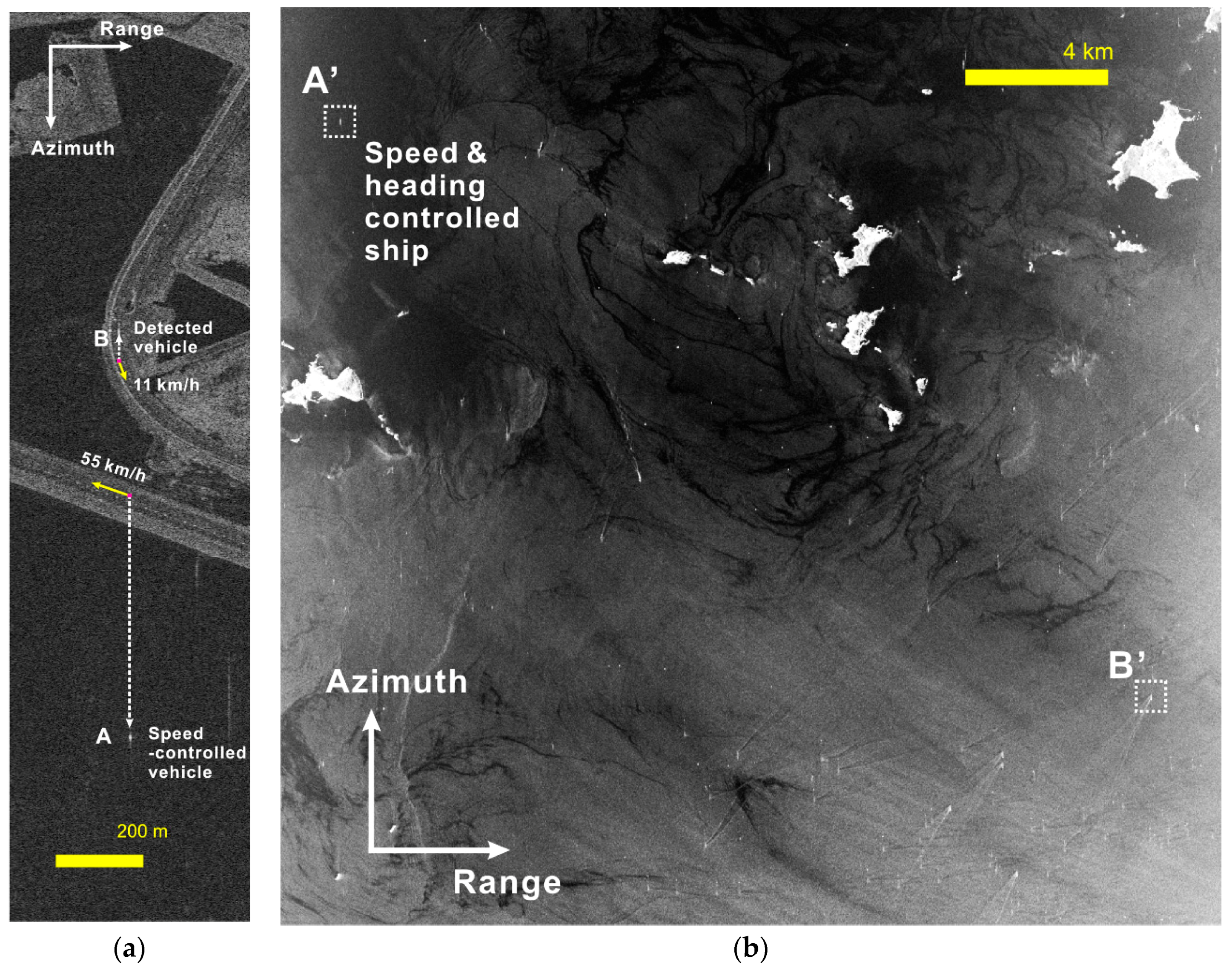
To evaluate the performance of the proposed method, it was applied to TerraSAR-X and KOMSAT-5 monostatic SAR data. System parameters of the two spaceborne SARs are summarized in Table 2. The first data were obtained by TerraSAR-X, when a speed-controlled vehicle was running on the road as an experiment, with velocities of −6.6 and −13.8 m/s (or −23.8 and −49.6 km/h, respectively), in the azimuth and range directions, respectively. Figure 1a shows the TerraSAR-X single-look complex (SLC) image used in this study, and the target denoted by “A” in Figure 1a represents the speed-controlled vehicle imaged at a shifted position, according to the range velocity component. The speed of the vehicle was precisely measured by GPS as well as a speedometer. The details of the data used in the test and the ground velocity of the vehicle are given in [35]. A corner reflector was mounted on the truck for the experiment, with a pre-designed deploying angle to maximize the returned SAR signal. This TerraSAR-X data was used for the estimation of the residual Doppler frequency of on-land ground moving targets by applying the proposed method.
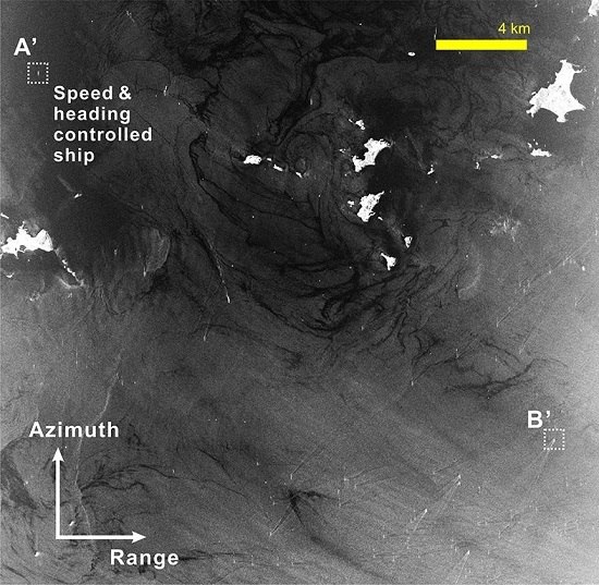
The method is also applied to the Korea Multi-Purpose Satellite -5 (KOMPSAT-5) monostatic SAR data, acquired over a coastal area as shown in Figure 1b. During the KOMSPAT-5 data acquisition, an experimental ship denoted by a square and “A’” in Figure 1b was cruising at a fixed heading and speed of 342.7°N and 16.4 km/h, respectively. One of the main purposes of the experiment was to evaluate the KOMPSAT-5 capability of slow-moving ships detection and velocity retrieval in the coastal region. The heading and velocity of the ship was precisely measured by an on-board GPS system.
Since the characteristics of targets and clutter are very different depending upon whether they are for land surface or in the sea, it is necessary to separately evaluate and validate the effectiveness of the proposed method each case.
3.2. On-Land Application Results
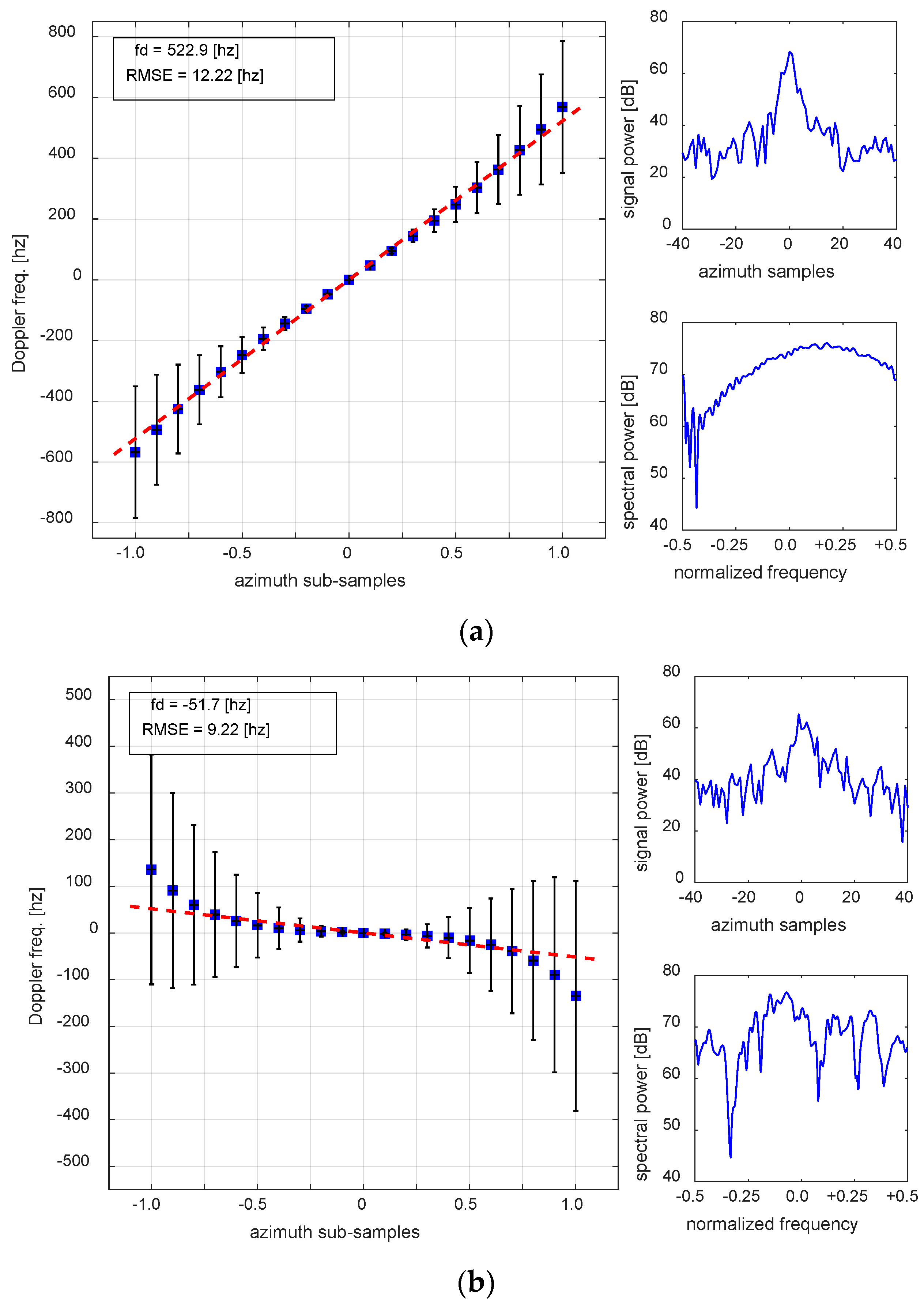
The application results for the ground moving targets of A and B, observed by TerraSAR-X in Figure 1a, are displayed in Figure 2. The result of the speed-controlled vehicle with a corner reflector, denoted by “A” in Figure 1a, is summarized in Figure 2a. The horizontal axis of the plot represents the azimuth subsamples described in Section 2.2. The azimuth subsamples (i.e., in Equation (2) or the temporal distance in the fraction of the azimuth sample time between the two signals) ranges from 0.1 up to 1.0 in a fraction of the original azimuth sample temporal distance. A total of only 41 samples were used for the estimation. The top right of each sub-figure presents the power of the signal, while the bottom right shows the Doppler spectrum.
Since the truck-mounted corner reflector was used for the experiment, the PSLR is high (−11.4 dB), with an SCR of 41.1 dB. When the PSLR and SCR is large enough, the phase interference from neighboring scatterers is not significant, and the variation of the Doppler frequency according to the azimuth temporal distance (or subsamples) aligns along a straight line with small perturbations. The estimated residual Doppler frequency is 522.9 Hz, with a root-mean-square error (RMSE) of 12.22 Hz, which corresponds to the range velocity of −51.4 ± 1.20 km/h. Since the ground truth range velocity of the vehicle is −49.6 km/h, the measurement error of the range velocity is only approximately −1.8 km/h or 3.5%. The results and errors obtained by the proposed method and conventional ESPRIT method are summarized in Table 3. The result demonstrates the effectiveness of the proposed method.
The conventional ESPRIT method applied to the same 41 samples produces a Doppler frequency estimation of 568.2 Hz, which is slightly overestimated. The conventional ESPRIT estimate corresponds to a range velocity of –55.8 km/h, so that an estimation error of –6 km/h or 12.5% in range velocity occurs. Thus, the proposed method is able to improve the residual Doppler frequency estimation from SAR SLC data by using only a limited number of samples.
The advantage of the proposed method is clear when it applies to general targets with weak radar returns. In the case of target, A in Figure 1a, it was deliberately pre-designed to be ideal for the experiment. The Doppler phase of the target remains intact from clutter because of the mounted corner reflector, and the Doppler spectrum reconstructed in Figure 1a (bottom right) also well-depicts the Doppler frequency spectrum. However, in the real world, the radar-returned signals from most on-land moving targets are generally by far weaker than the experimental vehicle, depending on the physical size, observation angles, materials, etc. More importantly, the experimental vehicle was deliberately imaged on the water surface to maximize the SCR. However, most ground moving targets are imaged on the land surface, which anticipates a small SCR. Even under such unfavorable on-land conditions, the proposed method is robust enough to provide the Doppler frequency with high precision, as shown in the example of Figure 2b. The result of the Doppler frequency estimation for the detected ground moving target, “B” in Figure 1a, is shown in Figure 2b. The vehicle was moving at low speed and the PSLR and SCR are only 7.4 dB and 27.3 dB, respectively. Compared with the target “A”, the Doppler frequency spectrum is also not clear enough to determine centre frequency. Under such conditions, it is very difficult to precisely estimate the Doppler frequency. The proposed method successfully estimated the residual Doppler frequency of –51.7 Hz, or equivalently, the range velocity at 5.1 ± 0.91 km/h. The range velocity can also be measured by the distance of the apparent shift of the target from the original position in the image, and the target “B” moved along a road with a range velocity of 5.9 km/h. Thus, the linear least squares estimation shows an error of –0.8 km/h or 13.6% of the range velocity. The conventional ESPRIT method simply provides the estimate of the last point (i.e., ) of the plot, and it overestimates as –134.4 Hz or equivalently 12.3 km/h—double the true values. As seen in Figure 2b, the Doppler frequency estimate does not increase linearly, but steeply, as the azimuth temporal distance increases. It accounts for the fact that the signals from a weak target are corrupted quickly by clutter as the temporal distance increases. Thus, it is necessary for the proposed method to be robust, even for weak targets and to include signals of high signal-to-noise ratio (SNR) only on linear least squares estimation. In this case, the estimation is done by satisfying a ratio () of Doppler frequency estimate to the root-mean-square error (RMSE) larger than 5.0. While the high ratio, the ideal target (A in Figure 1a) in Figure 2a, maintains up to , it is better for the weak target (B in Figure 1a) in Figure 2b to include points up to for the estimation.
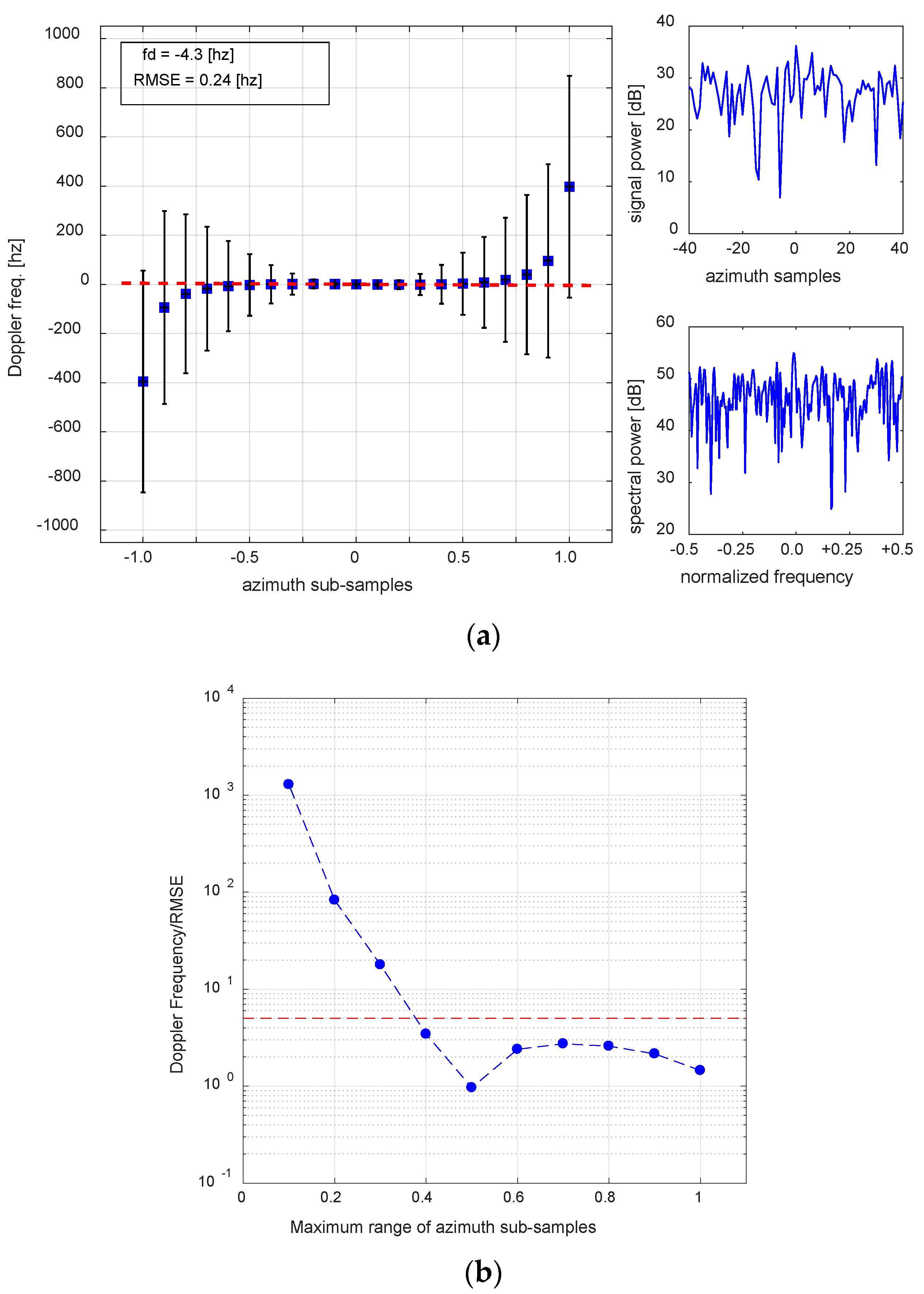
The ratio of is a very useful indicator for the estimation of the residual Doppler frequency, and the large values imply a significant residual Doppler frequency, with a small RMSE of the least squares. There is a trade-off between the RSME improvement and the increased bias created by limiting the maximum temporal distance. Thus, the question is how to determine the optimum ratio of for each estimation. This can be done by examining the behaviour of the Doppler frequency variation according to the azimuth temporal distance for a weak stationary target. Figure 3 is obtained by applying the method to a stationary weak target. The PSLR of the target is −4.3 dB, with an SCR of 9.6 dB. Since it is a stationary target, the residual Doppler frequency must be close to zero. However, the signal is very weak, and it is subject to phase corruption by clutter. The variation of the ratio versus the maximum azimuth subsamples is displayed in Figure 3b. As the azimuth temporal distance increases from 0.1 up to 1.0, the ratio decreases rapidly. The Doppler frequency estimate maintains stability near zero up to , but abruptly increases from 0.4. Thus, the ratio must be larger than that at , and Figure 3b suggests that the minimum value of ratio would be approximately 5 to 10 for on-land applications. In fact, this threshold value was applied for the estimation of Figure 2b (that is, the target “B” in Figure 1a). It must be stressed that this threshold value is only for the investigation of targets on land.
3.3. Application Results in Coastal Areas
On the residual Doppler frequency estimation of point targets in the sea, the characteristics of targets and clutter would be very different from those on land. Firstly, the size of the targets, for instance a ship, is usually larger than those on land. Secondly, the SCR in the sea is generally larger than that on land, although the SCR in the sea greatly depends on sea state and system parameters, including frequency and polarization. Thirdly, a ship or boat moving across the surface of the water produces a wake pattern that helps to detect and determine the direction of the movement. These three features make it easier to detect and estimate the residual Doppler frequency of moving targets in the sea. However, there are also some negative features to consider. Firstly, a forward speed of the ship is generally lower than that of vehicles on land, which implies that the residual Doppler frequency associated with target motion is relatively small and difficult to discriminate from clutter bandwidth. Secondly, roll and pitch are the most obvious motions of a ship, and they make scattering centers continuously move during SAR observation. For these reasons, some methods with specific tactics for ship detection, and its velocity estimation from space-borne SAR systems, have been developed. For instance, [36] proposed a sophisticated method utilizing clutterlock algorithm to improve ship detection and velocity retrieval. Ship wake-based techniques such as [44,45] also have become popular in coastal areas, and the measurement accuracy was less than 5% [45].
While a single dominant residual Doppler frequency associated with a forward motion of the ship is a primary concern, roll and pitch motions of a ship contribute to the instantaneous Doppler frequency components. Individual scattering centers at various parts of the ship differently experience instantaneous speeds of roll and pitch motion, and make the problem more complicated. Therefore, it is necessary to set up a different threshold value of the ratio for the coastal application of the proposed method.
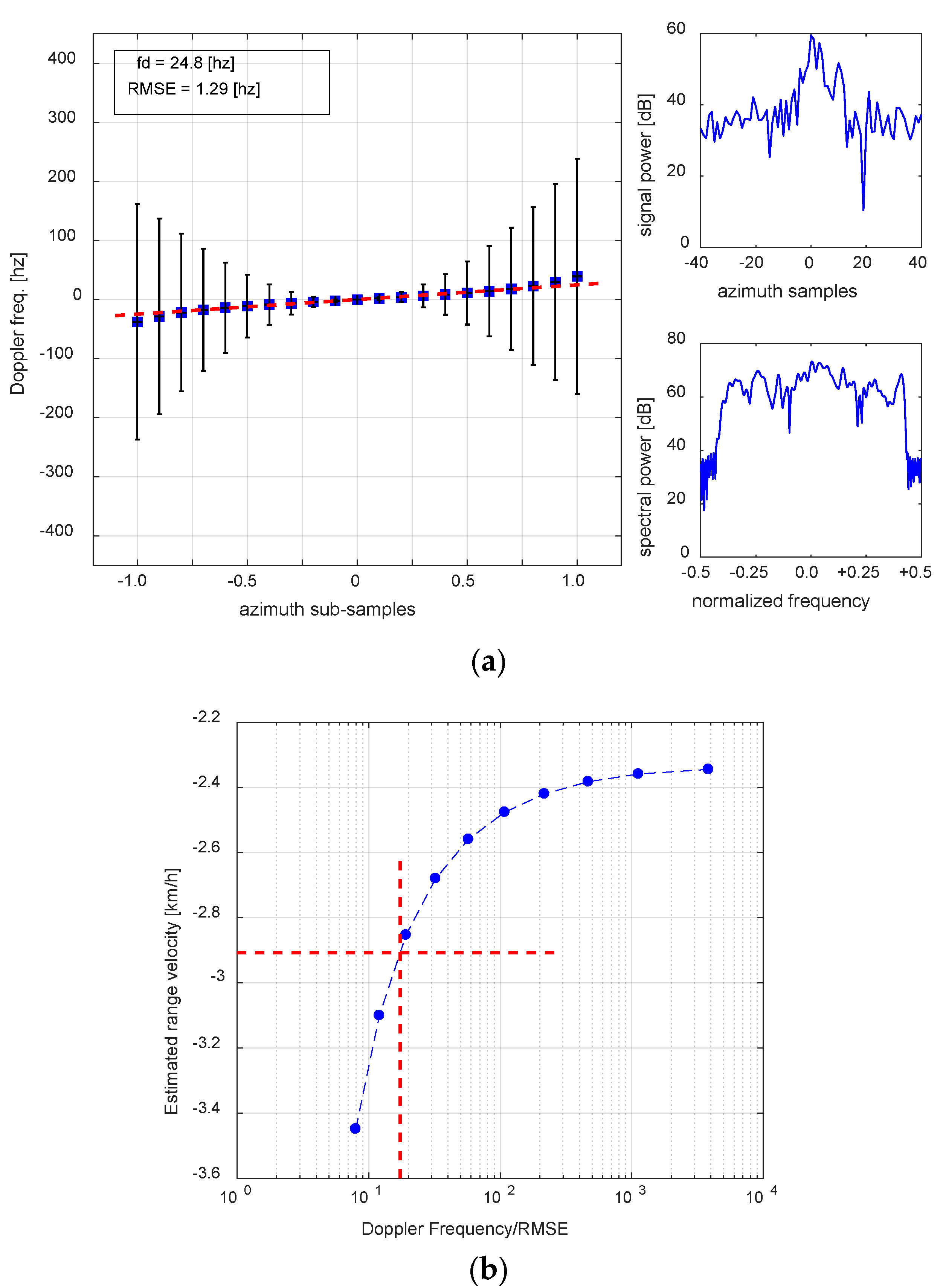
The speed and heading of the ship A’ in Figure 1b was particularly controlled for a ship detection experiment cruising at low speed. The range velocity of the ship was −2.9 km/h at the KOMPSAT-5 SAR observation angle. The PSLR of the target and SCR are −6.5 dB and 31.7 dB, respectively. The estimation results are in Figure 4. Comparing Figure 4 with Figure 2b and Figure 3, the large SCR of the targets in the sea makes the distribution of the residual Doppler frequency, according to the azimuth temporal distance, near linear. However, as discussed before, it requires higher measurement accuracy because of low speed and therefore, it is necessary to apply a stricter threshold value of the ratio than for on land.
It is difficult to determine the residual Doppler frequency from the Doppler spectrum of the ship in Figure 4a (right bottom). From the plot of Doppler frequency versus azimuth subsample (or azimuth temporal distance) in Figure 4a (left), the variation looks quasi-linear, but not exactly straight. Figure 4b is used to determine the optimum threshold ratio of Doppler frequency to RMSE as 17–20. Compared with the threshold value of 5–10 for the land speed study, the optimum ratio in the sea is at least double to triple the value for land. By applying the proposed method with a threshold of 17, the estimated range velocity of the ship is −2.85 ± 0.15 km/h, resulting in an estimation error of 1.7%. It is a very encouraging result, because it has previously been considered difficult to precisely measure a range velocity of less than 5 km/h by a single-channel SAR system [35].
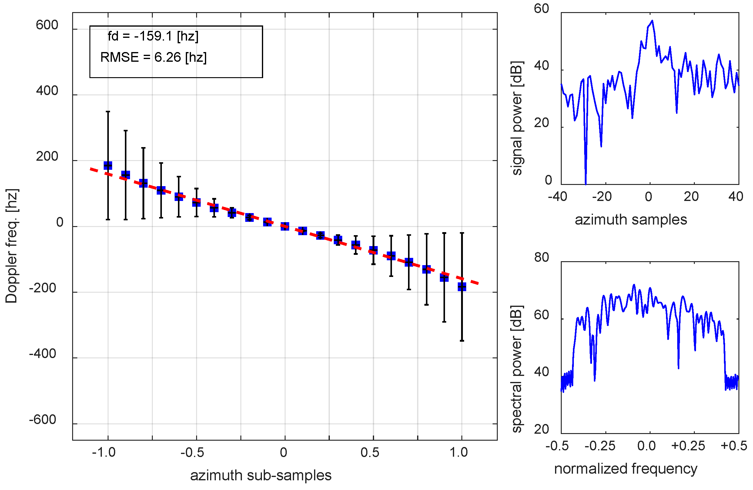
One high-speed ship with clear ship wake was selected to apply the method within the scene as denoted by “B’” in Figure 1b. The result with the threshold of 17 is summarized in Figure 5. Because of high SCR, the threshold would exclude only one or two points, but it would improve the measurement accuracy significantly. The ship B’ has a PSLR and RCS of −7.9 dB and 23.9 dB, respectively. The SCR is slightly lower than for ship A’, mainly because of ship wake. The estimated range velocity by this method is 18.3 ± 0.72 km/h. The range velocity can be estimated independently, by measuring the azimuth-shifted distance of the target from the apex of wake in the image, which provided a range velocity of 18.1 km/h. An absolute estimation error is 0.2 km/h or a percentage error of 1.1%.
The conventional ESPRIT for the same ship resulted in the range velocity of 20.9 km/h, which has an absolute estimation error of 2.8 km/h or a percentage error of 15.7%. Therefore, the exclusion of a few end points is very important to improve the measurement accuracy, with a strict threshold defined by ratio.
In summary, the proposed method is also very effective for the estimation of residual Doppler frequency and consequently range velocity with high precision in the coastal sea if a strict threshold of ratio is applied. The proposed method improves not only measurement accuracy, but also the single-channel SAR capability of monitoring moving targets in the sea even at low speed less than 5 km/h.
4. Discussion
To precisely measure a residual Doppler frequency of point target from monostatic SAR image data, it has been considered that the Doppler frequency must be significant and larger than the clutter bandwidth. Thus, it was only possible to detect and measure a fast-moving target with strong radar returns by the monostatic SAR. The lower limit was considered to be 5 km/h, with a PSLR −10 dB [35]. However, in practice, there are many artificial and natural point targets characterized by weakly returned signals and slow motion, particularly in the sea as well as on land. The proposed method demonstrates the competitive performance of precisely estimating slow-moving targets as slow as 2.9 km/h, even under conditions of a small PSLR and SCR. Thus, it extends the single-channel SAR capability for detection and measurement of slow-moving point targets. Estimation accuracy improvement is achieved by adopting linear least squares estimation with the inclusion of only intact azimuth subsamples, satisfying a certain threshold of the ratio, rather than a direct estimation of a fixed azimuth temporal distance of the original samples.
Although the effectiveness and efficiency of the proposed method is proven through the application examples, there are still some limitations of the method. First of all, the minimum range velocity required to accurately measure using this method is yet to be strictly defined.
Limits of PSLR and SCR on practical applications also exist. In previous studies, Park and Won [35] reported the limit of PSRL as −10 dB, based upon simulation results. In this study, the targets of PSLR less than −10 dB can also be successfully retrieved by trading-off increasing bias. The targets having lower PSLR and SCR produce a less accurate estimation. The in-depth study of the PSLR and SCR limitation was not examined in this study, and therefore they must be strictly defined in a future study.
In this paper, the optimum ratio threshold is recommended to be 7–10 and 17 for land and sea surface, respectively. However, these thresholds must be further reviewed for application because each SAR scene has different general conditions of PSLR and SCR. For instance, different sea states, urban versus rural areas, etc. A stationary point target would be useful for the analysis of each scene or area. A generalized critical value would be required after reviewing various monostatic SAR data and point targets within them.
When the SLC is used for the residual Doppler frequency estimation, it must be noted that the Doppler spectrum is normally band-limited because of a certain Doppler window applied by a SAR processor during image formation. The maximum Doppler bandwidth and the type of window (for instance, a general cosine window or hamming window), depend on the SAR processor used for focusing. It usually maintains approximately 80% of the original Doppler bandwidth in the normally processed SAR SLC data. This band-limited focused signal does not largely affect the Doppler frequency estimates by the ESPRIT algorithm for a stationary target because the applied Doppler window reduces the noise. However, for moving targets, this process undesirably removes the signal frequency components because the Doppler centre frequency of moving targets is shifted from the Doppler centroid of the scene. This usually results in underestimation of the residual Doppler frequency and consequently the range velocity for moving targets. Therefore, it is necessary to have an SAR processor maintaining the full bandwidth of the Doppler spectrum for a precise estimation of Doppler parameters from SAR SLC data.
In this study, it was not carried out for quantitative comparison of the results with those obtained by applying other methods to the same data. While the results provided in this paper was obtained from samples of one single range bin, other methods require at least a few tens of range bins for proper computation. Thus, a direct comparison between the results of this study with results of other method computed from a single range bin would not be appropriate. However, the Korea Institute of Ocean Science & Technology (KIOST) has a plan to carry out a field campaign with many ships of different sizes and moving speeds in the very near future, and quantitative and systematic comparison between different methods must be made when those field data are to be obtained.
5. Conclusions
For a precise estimation of residual Doppler frequency in single-channel SAR data, a new method is proposed, and its performance is demonstrated by applying TerraSAR-X and KOMPSAT-5 monostatic SAR data. The method succeeded in retrieving a range velocity as low as 2.9 km/h, while the estimation limit has previously been considered 5 km/h. Azimuth subsampling and linear least squares are core ideas of the proposed approach, which is able to provide an optimum estimation, even for slow-moving ground point targets under the unfavorable conditions of low PSLR and RCS. Estimation accuracy is significantly improved, particularly by introducing a threshold ratio, which results in excluding azimuth subsamples seriously affected by clutter. Since the characteristics of targets and clutter are very different on land and in the sea, the application of the method should be treated separately. The recommended thresholds are 7–10 and 17, for land and sea surface, respectively.
The proposed method would contribute to the extension of the monostatic SAR capability for detection and velocity retrieval of moving ground targets with a competitive accuracy. Compared with previously developed other methods, the proposed method would be more useful for small and slow-moving targets that extend only over a limited range bins. Although the basic performance of the method is demonstrated in this study, follow-up studies are required?particularly on the low bound of the range velocity, in-depth study of application restriction on PSLR and RCS, and critical threshold of the ratio for various targets and clutter conditions. For the proposed method to be fully proven, additional tests would be required using a large number of targets with different sizes and moving speeds, under various clutter environment in the near future.
Funding
This work was supported by the National Space Lab program through the Korea Science and Engineering Foundation, and partially supported by the Ministry of Science and Technology (2013M1A3A3A02042314) and by the Korea Institute of Marine Science & Technology Promotion (KIMST) in 2018 funded by the Ministry of Ocean and Fisheries (MOF) for a project of “Base research for building a wide integrated surveillance system of marine territory.”
Acknowledgments
The TerraSAR-X data were provided to J.S. Won as a part of the TerraSAR-X Science Team Project (PI No. COA0047). The KOMSAT-5 data and data of ship motion were acquired by the Korea Institute of Ocean Science & Technology (KIOST) in collaboration with Korea Aerospace Research Institute (KARI) as a part of a field campaign.
Conflicts of Interest
The author declares no conflict of interest.
References
- Goldstein, R.M.; Zebker, H.A. Interferometric radar measurement of ocean surface currents. Nature 1987, 328, 707–709. [Google Scholar] [CrossRef]
- Thompson, D.R.; Jensen, J.R. Synthetic aperture radar interferometry applied to ship-generated waves in the 1989 Loch Linnhe experiment. J. Geophys. Res. 1993, 981, 10259–10269. [Google Scholar] [CrossRef]
- Livingstone, C.; Sikaneta, I.; Gierull, C.H.; Chiu, S.; Beaudoin, A.; Campbell, J.; Beaudoin, J.; Gong, S.; Knight, T. An airborne SAR experiment to support RADARSAT-2 ground moving target indication (GMTI). Can. J. Remote Sens. 2002, 28, 749–813. [Google Scholar] [CrossRef]
- Breit, H.; Eineder, M.; Holzner, J.; Runge, H.; Bamler, R. Traffic monitoring using SRTM along-track interferometry. In Proceedings of the IGARSS 2003: 2003 IEEE International Geoscience and Remote Sensing Symposium, Toulouse, France, 21–25 July 2003; pp. 1187–1189. [Google Scholar]
- Gierull, C.H. Ground moving target parameter estimation for two-channel SAR. IEE Proc. Radar Sonar Navig. 2006, 153, 224–233. [Google Scholar] [CrossRef]
- Suchandt, S.; Runge, H.; Breit, H.; Steinbrecher, U.; Kotenkov, A.; Balss, U. Automatic extraction of traffic flows using TerraSAR-X along-track interferometry. IEEE Trans. Geosci. Remote Sens. 2010, 48, 807–819. [Google Scholar] [CrossRef]
- Chiu, S.; Dragosevi, M.V. Moving target indication via RADARSAT-2 multichannel synthetic aperture radar processing. EURASIP J. Adv. Signal Process. 2010, 2010, 740130. [Google Scholar] [CrossRef]
- Raney, R.K. Synthetic aperture imaging radar and moving targets. IEEE Trans. Aerosp. Electron. Syst. 1971, 7, 499–505. [Google Scholar] [CrossRef]
- Dickey, F.R.; Labitt, M.; Staudaher, F.M. Development of airborne moving target radar for long range surveillance. IEEE Trans. Aerosp. Electron. Syst. 1991, 27, 959–972. [Google Scholar] [CrossRef]
- Shnitkin, H. Joint stars phased array radar antenna. IEEE Trans. Aerosp. Electron. Syst. Mag. 1994, 9, 34–40. [Google Scholar] [CrossRef]
- Chiu, S.; Livingstone, C.E. A comparison of displaced phase centre antenna and along-track interferometry techniques for RADARSAT-2 ground moving target indication. Can. J. Remote Sens. 2005, 31, 37–51. [Google Scholar] [CrossRef]
- Cerutti-Maori, D.; Sikaneta, I. Generalization of DPCA processing for multichannel SAR/GMTI radars. IEEE Trans. Geosci. Remote Sens. 2013, 51, 560–572. [Google Scholar] [CrossRef]
- Ender, J.H.G. Space-time processing for multichannel synthetic aperture radar. Electron. Commun. Eng. J. 1999, 11, 29–38. [Google Scholar] [CrossRef]
- Melvin, W.L. A STAP overview. IEEE Aerosp. Electron. Syst. Mag. 2004, 19, 19–35. [Google Scholar] [CrossRef]
- Cerutti-Moari, D.; Gierull, C.H.; Ender, J.H.G. Experimental verification of SAR-GMTI improvement through antenna switching. IEEE Trans. Geosci. Remote Sens. 2010, 48, 2066–2075. [Google Scholar] [CrossRef]
- Chapman, R.D.; Hawes, C.M.; Nord, M.E. Target motion ambiguities in single-aperture synthetic aperture radar. IEEE Trans. Aerosp. Electron. Syst. 2010, 46, 459–468. [Google Scholar] [CrossRef]
- Kersten, P.R.; Topokov, J.V.; Ainsworth, T.L.; Sletten, M.A.; Jansen, R.W. Estimating surface water speeds with a single-phase center SAR versus an along-track interferometric SAR. IEEE Trans. Geosci. Remote Sens. 2010, 48, 3638–3646. [Google Scholar] [CrossRef]
- Chen, C.C.; Andrews, H.C. Target motion induced radar imaging. IEEE Trans. Aerosp. Electron. Syst. 1980, 16, 2–14. [Google Scholar] [CrossRef]
- Barbarossa, S. Detection and imaging of moving objects with synthetic aperture radar—Part I: Optimal detection and parameter estimation theory. IEE Proc. F Radar Signal Process. 1992, 139, 79–88. [Google Scholar] [CrossRef]
- Petterson, M.I.; Sjogren, T.K.; Vu, V.T. Performance of moving target parameter estimation using SAR. IEEE Trans. Aerosp. Electron. Syst. 2015, 51, 1191–1201. [Google Scholar] [CrossRef]
- Park, J.-W.; Kim, J.H.; Won, J.-S. Fast and efficient correction of ground moving targets in a synthetic aperture radar, single-look complex image. Remote Sens. 2017, 9, 926. [Google Scholar] [CrossRef]
- Statman, J.I.; Rodemich, E.R. Parameter estimation based on Doppler frequency shifts. IEEE Trans. Aerosp. Electron. Syst. 1987, 23, 31–39. [Google Scholar] [CrossRef]
- Freeman, A.; Currie, A. Synthetic aperture radar (SAR) images of moving targets. GEC J. Res. 1987, 5, 106–115. [Google Scholar]
- Barbarossa, S.; Farina, A. Space-time-frequency processing of synthetic aperture radar signals. IEEE Trans. Aerosp. Electron. Syst. 1994, 30, 341–358. [Google Scholar] [CrossRef]
- Kersten, P.R.; Jansen, R.W.; Luc, K.; Ainsworth, T.L. Motion analysis in SAR images of unfocused objects using time-frequency methods. IEEE Geosci. Remote Sens. Lett. 2007, 4, 527–531. [Google Scholar] [CrossRef]
- Sparr, T. Moving target motion estimation and focusing in SAR images. In Proceedings of the IEEE Radar Conference, Arlington, VA, USA, 9–12 May 2005; pp. 290–294. [Google Scholar] [CrossRef]
- Li, F.-K.; Held, D.N.; Curlander, J.C.; Wu, C. Doppler parameter estimation for spaceborne synthetic-aperture radars. IEEE Trans. Geosci. Remote Sens. 1985, 23, 47–56. [Google Scholar] [CrossRef]
- Madsen, S.N. Estimating the Doppler centroid of SAR data. IEEE Trans. Aerosp. Electron. Syst. 1989, 25, 134–140. [Google Scholar] [CrossRef] [Green Version]
- Bamler, R. Doppler frequency estimation and the Cramer-Rao bound. IEEE Trans. Geosci. Remote Sens. 1991, 29, 385–390. [Google Scholar] [CrossRef]
- Wong, F.; Cumming, I.G. A combined SAR Doppler centroid estimation scheme based upon signal phase. IEEE Trans. Geosci. Remote Sens. 1996, 34, 696–707. [Google Scholar] [CrossRef]
- Cumming, I.G. A spatially selective approach to Doppler estimation for frame-based satellite SAR processing. IEEE Trans. Geosci. Remote Sens. 2004, 42, 1135–1148. [Google Scholar] [CrossRef] [Green Version]
- Li, Y.; Fu, H.; Kam, P.Y. An improved Doppler parameter estimator for synthetic aperture radar. PIERS Online 2008, 4, 201–206. [Google Scholar] [CrossRef]
- Li, W.; Yang, J.; Huang, Y. Improved Doppler parameter estimation of squint SAR based on slope detection. Int. J. Remote Sens. 2014, 35, 1417–1431. [Google Scholar] [CrossRef]
- Marques, P.A.C.; Dias, J.M.B. Velocity estimation of moving targets using a single SAR sensor. IEEE Trans. Aerosp. Electron. Syst. 2005, 41, 75–89. [Google Scholar] [CrossRef]
- Park, J.-W.; Won, J.-S. An efficient method of Doppler parameter estimation in the time–frequency domain for a moving object from TerraSAR-X data. IEEE Trans. Geosci. Remote Sens. 2011, 49, 4771–4787. [Google Scholar] [CrossRef]
- Renga, A.; Moccia, A. Use of Doppler parameters for ship velocity computation in SAR images. IEEE Trans. Geosci. Remote Sens. 2016, 54, 3995–4011. [Google Scholar] [CrossRef]
- Roy, R.; Paulraj, A.; Kailath, T. ESPRIT—A subspace rotation approach to estimation of parameters of cisoids in noise. IEEE Trans. Acoust. Speech Signal Process. 1986, 34, 1340–1342. [Google Scholar] [CrossRef]
- Roy, R.; Kailath, T. ESPRIT-estimation of signal parameters via rotational invariance techniques. IEEE Trans. Acoust. Speech Signal Process. 1989, 37, 984–995. [Google Scholar] [CrossRef]
- Schmidt, R. Multiple emitter location and signal parameter estimation. IEEE Trans. Antennas Propag. 1986, 34, 276–280. [Google Scholar] [CrossRef]
- Stoica, P.; Moses, R.L. Spectral Analysis of Signals, 1st ed.; Prentice-Hall: Upper Saddle River, NJ, USA, 2005; ISBN 0-13-113956-8. [Google Scholar]
- Santamaria, I.; Pantaleon, C.; Ibanez, J. A comparative study of high-accuracy frequency estimation methods. Mech. Syst. Signal Process. 2010, 14, 819–834. [Google Scholar] [CrossRef]
- Krieger, G.; Gebert, N.; Moreira, A. Unambiguous SAR signal reconstruction from nonuniform displaced phase center sampling. IEEE Geosci. Remote Sens. Lett. 2004, 1, 260–264. [Google Scholar] [CrossRef]
- Eigenvalues and Eigenvectors of 2 × 2 Matrices. Available online: http://www.math.harvard.edu /archive/21b_fall_04 /exhibits/2dmatrices/index.html (accessed on 23 May 2018).
- Graziano, M.D.; D’Errico, M.; Rufino, G. Wake component detection in X-Band SAR images for ship heading and velocity estimation. Remote Sens. 2016, 8, 498. [Google Scholar] [CrossRef]
- Panico, P.; Graziano, M.D.; Renga, A. SAR-based vessel velocity estimation from partially imaged Kelvin pattern. IEEE Geosci. Remote Sens. Lett. 2017, 14, 2067–2071. [Google Scholar] [CrossRef]
Figure 1.
Two synthetic aperture radar (SAR) images used in this study: (a) TerraSAR-X SLC image, in which a speed-controlled vehicle A is observed. (b) KOMPSAT-5 SLC image over coastal areas, in which a speed and heading controlled ship A’ for the experiment, as well as numerous high velocity ships, are observed.

Figure 2.
(a) Residual Doppler frequency estimation of the speed-controlled vehicle denoted by “A” in Figure 1a. The SAR-measured range velocity by the proposed method is −51.4 ± 1.20 km/h, while that recorded by GPS on the car is 49.6 km/h. The peak-to-sidelobe ratio (PSLR) of the vehicle is −11.4 dB, with a signal-to-clutter ratio (SCR) of 41.1 dB. (b) Residual Doppler frequency estimation of the detected target “B” in Figure 1a. The SAR measured range velocity is approximately 5.1 ± 0.91 km/h, with an azimuth velocity of approximately 9.8 km/h. The PSLR of the target is −7.4 dB, with an SCR of 27.3 dB. While the Doppler spectrum (bottom right in each sub-figure) of targets with high PSLR and SCR well-depicts the Doppler centre frequency as in (a), it is difficult to determine a centre frequency from the Doppler spectrum of weak point targets, as seen in (b).

Figure 3.
An application result for a weak stationary target, to determine an optimum ratio of Doppler frequency to RMSE for estimation on land. The PSLR of the target is −4.3 dB, with an SCR of 9.6 dB. A ratio of larger than 5–10 would be acceptable for the on-land point targets.
Figure 3.
An application result for a weak stationary target, to determine an optimum ratio of Doppler frequency to RMSE for estimation on land. The PSLR of the target is −4.3 dB, with an SCR of 9.6 dB. A ratio of larger than 5–10 would be acceptable for the on-land point targets.

Figure 4.
Results from the ship for the experiment denoted by “A’” in Figure 1b. The ship velocity measured by on-board GPS at the time of SAR data acquisition was 16.4 km/h with an azimuth and range component of 16.1 and 2.91 km/h, respectively. The PSLR and SCR are −6.5 dB and 31.7 dB, respectively. The estimated residual Doppler frequency of 24.8 Hz corresponds to the range of −2.85 ± 0.15 km/h. From this analysis, the optimum ratio of Doppler frequency to RMSE in the sea is determined as 17.

Figure 5.
The SAR measured Doppler frequency of the high-speed ship B’ in Figure 1b. The corresponding range velocity is 18.3 ± 0.72 km/h. The PSLR and SCR of the target are −7.9 dB and 23.9 dB, respectively. The estimated range velocity by this method was confirmed by measuring the azimuth distance of the target, shifted from the apex of wake in the image.


Table 1.
Pseudocode of the proposed algorithm.
| Linear Least Squares Algorithm Pseudocode |
|---|
| Input: Output: Initialize the accumulator to zero Define a total of (2N + 1) time symmetric ← FFT of for all do ← Multiply to ← IFFT of Estimate by ESPRIT method ← end for Compute ← diving by sum of squares , Equation (12) return |
Table 2.
SAR system parameters used in this study.
| Parameter | TerraSAR-X | KOMPSAT-5 |
|---|---|---|
| Wavelength | 3.1 cm | 3.1 cm |
| Polarization | HH | HH |
| PRF | 3815.5 Hz | 3787.9 Hz |
| Antenna velocity | 7686.5 m/s | 7664.5 m/s |
| Antenna size | 4.8 m | 4.5 m |
| Incidence angle | 39.25° | 33.55° |
| Altitude | 513.1 km | 557.5 km |
Table 3.
Summary of application results.
| Area | Target ID | Reference Range Velocity [km/h] | Range Velocity by Proposed Method [km/h] | Error [km/h] | Doppler Freq./RMSE Ratio | Range Velocity by ESPRIT [km/h] | Error [km/h] |
|---|---|---|---|---|---|---|---|
| Land | A | −49.6 | −51.4 ± 1.20 | 1.8 | 42.8 | −55.8 | 6.2 |
| B | 5.9 1 | 5.1 ± 0.91 | 0.9 | 5.6 | 12.3 | 6.4 | |
| Sea | A’ | −2.9 | −2.85 ± 0.15 | 0.05 | 19.2 | −4.4 | 1.5 |
| B’ | 18.1 1 | 18.3 ± 0.72 | 0.2 | 25.4 | 20.9 | 2.8 |
1 Estimated from the distance of the apparent shift in the image.
© 2018 by the author. Licensee MDPI, Basel, Switzerland. This article is an open access article distributed under the terms and conditions of the Creative Commons Attribution (CC BY) license (http://creativecommons.org/licenses/by/4.0/).
Share and Cite
MDPI and ACS Style
Won, J.-S. Doppler Frequency Estimation of Point Targets in the Single-Channel SAR Image by Linear Least Squares. Remote Sens. 2018, 10, 1160. https://doi.org/10.3390/rs10071160
AMA Style
Won J-S. Doppler Frequency Estimation of Point Targets in the Single-Channel SAR Image by Linear Least Squares. Remote Sensing. 2018; 10(7):1160. https://doi.org/10.3390/rs10071160
Chicago/Turabian StyleWon, Joong-Sun. 2018. "Doppler Frequency Estimation of Point Targets in the Single-Channel SAR Image by Linear Least Squares" Remote Sensing 10, no. 7: 1160. https://doi.org/10.3390/rs10071160
Note that from the first issue of 2016, this journal uses article numbers instead of page numbers. See further details here.