Estimation of Gap Fraction and Foliage Clumping in Forest Canopies


1
Tartu Observatory, University of Tartu, 61602 Tõravere, Estonia
2
Institute of Forestry and Rural Engineering, Estonian University of Life Sciences, Kreutzwaldi 5, 51014 Tartu, Estonia
3
Department of Civil Engineering and Architecture, Road Engineering and Geodesy Research Group, Tallinn University of Technology, Ehitajate tee 5, 19086 Tallinn, Estonia
*
Author to whom correspondence should be addressed.
Remote Sens. 2018, 10(7), 1153; https://doi.org/10.3390/rs10071153
Submission received: 14 May 2018
/
Revised: 31 May 2018
/
Accepted: 18 July 2018
/
Published: 21 July 2018
(This article belongs to the Special Issue Optical Remote Sensing of Boreal Forests)
Abstract
:The gap fractions of three mature hemi-boreal forest stands in Estonia were estimated using the LAI-2000 plant canopy analyzer ( LI-COR Biosciences, Lincoln, NE, USA), the TRAC instrument (Edgewall, Miami, FL, USA), Cajanus’ tube, hemispherical photos, as well as terrestrial (TLS) and airborne (ALS) laser scanners. ALS measurements with an 8-year interval confirmed that changes in the structure of mature forest stands are slow, and that measurements in the same season of different years should be well comparable. Gap fraction estimates varied considerably depending on the instruments and methods used. None of the methods considered for the estimation of gap fraction of forest canopies proved superior to others. The increasing spatial resolution of new ALS devices allows the canopy structure to be analyzed in more detail than was possible before. The high vertical resolution of point clouds improves the possibility of estimating the stand height, crown length, and clumping of foliage in the canopy. The clumping/regularity of the foliage in a forest canopy is correlated with tree height, crown length, and basal area. The method suggested herein for the estimation of foliage clumping allows the leaf area estimates of forest canopies to be improved.
1. Introduction
Radiative transfer and (directional) reflectance of vegetation canopies determine the energy budget, photosynthesis, and possibilities of the remote monitoring of vegetation canopies. In the radiative transfer in a vegetation canopy, transmittance has a key role in direct radiation and the chance of a photon to escape—the gap fraction in the view and/or Sun direction in the canopy. For the analysis of the structure of low vegetation covers, the point quadrat method was suggested a long time ago [1]. Thin needles are passed vertically through vegetation, and the number of contacts between needles and foliage is recorded. Sometimes records are made of only the first contact made by a point quadrat. The percentage of quadrats which make contact is termed “percent cover”, and the percentage of quadrats which have no contact is called the “gap fraction”. Refs. [2,3] analyzed the point quadrat method and possible errors associated with the method. The method of point quadrats cannot be directly applied for the study of forest canopy. Indirect methods have been used instead. These include:
Each of these methods has its limitations. Measurements with the Cajanus tube are labor-intensive, and are typically used for the estimation of vertical canopy cover in forests [6,7,8]. The LAI-2000 plant canopy analyzer allows the measurement of gap fraction in five intervals of zenith angle averaged over azimuth. Hemispherical photos allow a more detailed analysis of the gap fraction of the canopy than the LAI-2000. Numerous studies have investigated the estimation of gap fraction using the LAI-2000 or hemispherical photographs (e.g., Chen et al. [9], Jonckheere et al. [10], Cescatti [11], Lang et al. [12], Pisek et al. [13], Glatthorn and Beckschäfer [14], Woodgate et al. [15], Kuusk [16], among others).
As demonstrated by Kuusk [16], LAI-2000 gap fraction (and leaf area index, LAI) estimates are biased. The bias depends on the LAI and the leaf angle distribution (LAD) in the canopy. Since calibration against LAI-2000 is rather common practice in determining the gap fraction from hemispherical photos, or if some other method based on the pixel intensity is applied, a bias similar to that of LAI-2000 is possible.
With the TRAC instrument, direct sunrays assume the role of the thin needle of point quadrats. The range of sun zenith angles at the study site determines the possible range of gap fraction analysis. A disturbing problem is the precence of penumbra caused by the finite angular size about 30’ of the Sun disk.
Laser scanners, both terrestrial and airborne, provide additional possibilities to analyze forest canopy structure. Attempts to study forest structure, specifically the angular profiles of gap fraction , by terrestrial laser scanners started in the beginning of the previous decade. Attempts by Danson et al. [17,18,19] demonstrated good agreement of TLS and the photographic method in a pine forest, but large differences in a broadleaf forest—TLS gap fraction estimates were about half of those from hemispherical photos. Calders et al. [20] discovered that, although relatively similar patterns could be detected between the shapes of the gap fraction curves, gap fraction distributions derived from TLS were consistently lower than the values obtained from hemispherical photography. Seidel et al. [21] compared TLS and HP techniques using measurements in 35 scan positions in old-growth forest patches. Correlation of HP and TLS values was high, r = 0.76. However, TLS values were systematically lower, . The analysis by Kuusk [16] hints that the gap fraction values determined by passive optical techniques such as LAI-2000 and HP may be overestimated by 10–20% in stands of moderate density. Considering such an overestimate in the gap fraction from HP-s, the regression by Seidel et al. [21] becomes at .
In this study, the gap fraction in three exhaustively studied mature hemi-boreal forest stands, two of which served as targets during the fourth radiation transfer model intercomparison (RAMI-IV) [22], was estimated using different methods. ALS data of multiple discrete returns were also used for the estimation of foliage clumping in forest canopies. Dependence of the estimated clumping factor on forest mensuration parameters was analyzed using ALS data over about two hundred homogeneous hemi-boreal forest stands.
2. Materials and Methods
2.1. Test Site
This study was carried out in Northern Europe, Estonia, at the Järvselja Training and Experimental Forestry District (58.30N, 27.26E). Järvselja forests, located on a flat landscape at 50 m above sea level, are representative of the hemi-boreal zone. Stands are pure or mixed, and are composed mainly of silver birch (Betula pendula Roth), Scots pine (Pinus sylvestris L.), Norway spruce (Picea abies (L.) Karst.), common alder (Alnus glutinosa (L.) Gaertn.), aspen (Populus tremula L.), white alder (Alnus incana (L.) Moench), small-leaved lime (Tilia cordata Mill.). Growth conditions range from poor, where the site index (stand height at the stand age of 100 years) is less than 10 m, to very good, where can be over 35 m. A more detailed description of the test site was provided by Kuusk et al. [23]. To update information for forest management planning, inventories of forest stands in Järvselja are carried out with a cycle of about ten years by licensed forest inventory experts. The information is stored and updated in stand maps and in a description database. The GIS database from the forest inventory conducted in 2011 contains several forest parameters, such as species composition, age, diameter at breast-height, tree height, site type, etc., for each stand. A forest stand is defined as a geographically unified area which has a relatively uniform tree species composition and is managed as a single unit. Three mature stands at the test site have been studied in detail previously, and the database of the forest structure and optical properties that is intended for forest radiative transfer modeling experiments, referred to as the Järvselja database, was built by [7,8]. The three stands are here referred to as RAMI stands. A basic description of these stands is given in Table 1. Canopy cover is the proportion of canopy overlying the forest floor. Crown cover is the ratio of total area of crown projections to the plot area. All trees with a trunk diameter at breast height larger than 4 cm were tallied. A detailed description of stand structure measurements was given by Kuusk et al. [7] and in the Technical Report [8].
2.2. Measurements
The methods for gap fraction estimation named in the introduction were tested in three RAMI stands. Several other stands were measured with ALS in 2017.
2.2.1. Ground-Based Measurements
Ground-based measurements of canopy cover and gap fraction have been carried out in RAMI stands in different years using various instruments [7,8].
The Cajanus tube was used to obtain canopy cover and crown cover estimates in RAMI stands in summer 2007 according to the methodology by Korhonen et al. [6]. About 350 samples were taken in every stand using random line transect sampling.
LAI-2000 measurements were carried out in RAMI stands on a regular grid of nine sample points L1–L9, with a grid step of 30 m. The relative coordinates of grid vertexes in a 100 × 100 m stand were = 20, 50, 80 m. Measurements were acquired in all three RAMI stands in July 2007 and July 2009. Recorded gap fraction values were corrected for bias by specular reflection on canopy leaves or needles according to the methodology by Kuusk [16]. In gap fraction measurements, leaves, needles, and other plant material are not distinguished.
TRAC measurements were acquired in RAMI stands in July 2009 in the range of sun zenith angles 37–79°.
Digital hemispherical photos using a Nikon Coolpix-4500 camera equipped (Nikon Inc., Tokyo, Japan) with hemispherical adapter FC-E8, and a Canon 5D camera (Canon Inc., Tokyo, Japan) with Sigma 8 mm, F3.5 EX DG optics were acquired in July 2007, July 2009, and August 2013. Data were stored in raw format and further processed according to Lang et al. [12]. Digital cameras have an RGB color filter array where the signal from blue pixels of the sensor is linearly comparable to the LAI-2000 readings [11]. Such cameras have a very high angular resolution in comparison with the LAI-2000 PCA. Two calibrated digital hemispherical cameras can be operated in the same manner as two LAI-2000 sensors—one as a reference in an open place and the other below the canopy. In practical measurement experiments in forests, it can be problematic to find a nearby, sufficiently large open area for the reference device. Therefore, the above-canopy sky reference is generated from below-canopy images using the camera signal in canopy gaps. Thus, gap fraction measurements were conducted using a single digital hemispherical camera that is capable of storing raw sensor data [12].
Measurements with a discrete return Leica ScanStation C10 terrestrial laser scanner were carried out in RAMI stands in August 2013. The main technical specifications of the instrument are as follows [24]:
- Scanning range 0.5–300 m.
- Horizontal scanning range of 360°, vertical scanning range at least 270°.
- Laser wavelength 532 nm. Size of the laser beam not more than 7 mm at a distance of 50 m.
- Accuracy of target measurements at least 2 mm within a distance of 50 m.
Measurements were acquired at LAI points L1–L9, and additionally in five points around the central LAI point L5 in the pine and birch stands. TLS data resolution was set to cm at the distance of 100 m on a perpendicular surface. Since the scanner spreads out measuring beams radially from its location, the point cloud can be as dense as mm at the distance of 5 m. On the other hand, there are data gaps in the sectors that are shadowed by the first object (leaf or a tree stem) in the path of the laser beam. In order to reduce the size and inhomogeneity of the point cloud, a discrete space of m was used. Voxels of 1 cm size were described by a binary function having value 0 if the voxel was empty, and value 1 otherwise. The scanner records hits, and there is no information about the pulses which had no hits. Therefore, two procedures were applied for the estimation of gap fraction. In the first procedure the discrete space of polar coordinates with cell size () was used. The polar coordinates () of every non-empty voxel were found, and the polar cells which correspond to the hits were assigned the value . The average gap fraction was estimated by averaging directional gap fraction over azimuth in the interval of zenith angles °. In order to avoid systematic errors in the estimated gap fraction, the discretization of the polar space must correspond to the polar steps of the scanner.
In the second procedure, the thresholded image of a digital hemispherical camera was simulated. The hemisphere was projected onto the rectangular grid as in the digital camera equipped with a hemispherical lens. For every voxel with hits, the corresponding pixel of the hemispherical photo was assigned the value 1. The pixels of the simulated image on which no hits were projected had the value 0. The average value of pixels in the range of zenith angles was the estimated probability of hits averaged over azimuth.
2.2.2. Airborne Measurements
Measurements with an airborne laser scanner (ALS) over the test site were carried out twice. On 30 August 2009, the three RAMI stands were measured with a Leica ALS50-II discrete return airborne laser scanner. The ALS has a near-infrared (NIR) laser transmitter, the output beam divergence is of 0.22 mr at the level. The system is capable of detecting up to four discrete returns for each outbound laser pulse. Vertical discrimination distance is approximately 3.5 m. Flight height was 500 m, every stand was crossed twice at perpendicular directions, the total point density was about 20 pulses per square meter, and the estimated hit position accuracy 6 cm.
On 16 June 2017, the test site was measured with a Riegl VQ-1560i waveform ALS [25]. The ALS has a wavelength of 1064 nm, pulse duration 3 ns, beam divergence 0.25 mr, accuracy 20 mm, and registers up to 15 targets per laser pulse. The test site was measured from the height of 350 m, and pulse density was 110 m. The RAMI stands were scanned twice, resulting in a total pulse density of 220 m.
Lang et al. [26] compared the estimates of ground surface height in 61 forest stands at the test site using both the Leica and Riegl instruments. Differences were marginal—mean differences were less than 1 cm if the surface height was estimated from the profiles of first hits.
The number of sounding pulses and the range of zenith angles over the 100 × 100 m stands were 0.2 millions and 0–6° in 2009, 2.2 millions and 0–9° in 2017. Altogether about 200 homogeneous and sufficiently large stands which were located on the flight paths close to the three RAMI stands were measured in 2017. The view zenith angles could reach up to 30°.
The test site and the ALS measurements are depicted in Figure 1.
The Riegl VQ-1560i ALS is able to fix a target of 20% reflectivity at a distance of 1700 m [25]. Therefore, at a distance of 350 m a target of 20% reflectivity which fills 4% of the beam cross-section should be recordable. At a 350 m flight height, the footprint of the beam has a diameter of about 9 cm and an area of 60 cm, and thus a discrete return can be caused by a target of about 2 cm area.
A needle probe of finite diameter causes a biased estimate of gap fraction in point quadrats [3]. A similar situation occurs in ALS measurements—the laser beam of finite diameter results in an underestimated gap fraction. The bias can be estimated by a simple theoretical experiment. If there is a circular test area of unit size , where radius , we get hits of point quadrats with a needle of infinitely small diameter, , where p is the plot cover and is the density of tests, respectively. The probe needle of diameter R will have hits at the area , the number of hits will be , and the estimate of hit probability
is biased. Therefore, a sounding beam of 9 cm in diameter causes an overestimation of cover by about 20%.
Specification of the RIEGL ALS allows up to 15 recorded hits per pulse. However, in the data acquired there were only some occasions of five hits; nearly all pulses had one to four hits. The cumulative histogram (distribution function) of ALS hits as a function of the height in the RAMI pine stand is plotted in Figure 2. The curves depicted correspond to the distribution of first hits, last hits, all hits, and the weighted distribution of hits when the hits were counted with weights , where is the number of discrete returns of the pulse. The horizontal line m marks the analyze level. The intersections of the distribution curves with the analyze level are the probabilities of hits below the level . In the pine stand, tree stems are disbranched, the live crown base of trees is between 11 and 13 m, and there is no undergrowth. Therefore, the probabilities had almost no sensitivity on the analyze level in the range of heights 0.5–10 m. That is, laser hits were on the ground or in tree crowns at 10–20 m. About 26% of first hits reached ground. Thus, the probability of gaps of diameter no less than the beam diameter (9 cm) was 26%, while only 20% of last hits were at a height of 2 m or more from the ground. Recall that already a 2 cm object with reflectance of 20% can trigger a hit. A better estimation of gap fraction is the probability of all hits which reach the level —46% in the pine stand. In the case of several discrete returns, one target does not intercept the whole beam. If all hits are at the same side of the reference level, then they contribute to the gap or cover probability. Otherwise, the contribution of a hit can be weighted by the inverse number of hits of the pulse. This probability is plotted in Figure 2 as well, and it exceeds the near-vertical gap probability estimate of all hits by 5%.
The high vertical resolution of RIEGL ALS profiles allows a more detailed analysis of the vertical profiles of hits. The waveform profiles were sampled with a time step of 1 ns, and therefore the discrete returns of a pulse could not be closer to each other than 0.3 m. If we extracted a horizontal layer of thickness m from the canopy, then there would be no mutually shadowing canopy elements for the scanner in that layer. The transparency of the elementary layer is , where is the probability of a hit in the layer . If the patterns of canopy elements in differential layers were independent, then the gap probability of the canopy would be
where H is the stand height, and is the transparency of layer at the level .
The gap fraction of the foliage layer of the leaf area index L is [27]
where is the Ross–Nilson geometry function (the projection of the unit area of foliage in the view direction), c is the clumping/regularity parameter, and is the zenith angle. As the view direction for these measurements is close to vertical, the gap fraction expression can be simplified:
The gap fraction estimate Equation (2) was calculated with the assumption of independence of elementary layers. That is, the clumping parameter c in Equation (4) corresponds to a random structure, . Equations (2) and (4) allow estimation of the clumping parameter c in a forest stand:
On the other hand, if we know the geometry function in the canopy and estimate the value of the clumping parameter c from Equation (5), we can estimate the LAI of the stand:
3. Results
3.1. Gap Fraction in Forest Stands
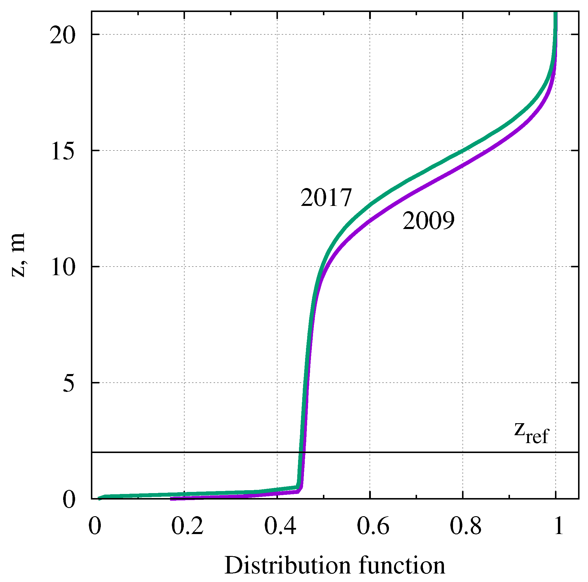
Changes in the crown layer structure of mature forest stands from year to year are small. The only change in the vertical distribution of ALS hits in the pine stand during eight years from 2009 to 2017 was the shift of tree crowns by 0.7 m up (Figure 3). There was almost no change in either the gap fraction at ground or in the shape of the distribution. According to the ground-based hypsometer measurements by Lang et al. [28] in 2016, the mean stand height and height to live crown base had increased by 1.1 m since 2007.
In the birch stand the undergrowth had grown up to about 5 m (Figure 4). Trees were taller and tree crowns had grown longer. The gap fraction in the crown layer had almost no change. The changes were most remarkable in the spruce stand (Figure 5). The gap fraction of the whole canopy had some increase, trees grew taller, and tree crowns longer.
Gap fraction data acquired in the same season of different years are well comparable. Much more problematic are the differences in gap fraction estimates obtained using different equipment and different methods.
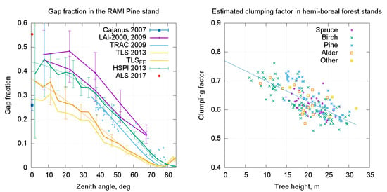
The estimates of gap fraction in the RAMI stands using different equipment and methods are provided in Figure 6 . The measurements with Cajanus’ tube and ALS provide gap fraction estimates in zenith direction only. TRAC measurements are limited by the range of sun zenith angles at the site. Measurements with LAI-2000, TLS, and hemispherical photos provide gap fraction estimates in the whole range of zenith angles from 0° to 90°, however uncertainty is high near zenith due to insufficient averaging.
The gap fraction data at zenith acquired with Cajanus’ tube were collected in July 2007.
LAI-2000 measurements were from 2009. Two instruments were used. In the pine stand, the measurements were done using two different procedures. The field restrictor of 180° was used. Four samples were taken with both instruments near every LAI point L1 to L9. The azimuth of one instrument was kept equal to the reference instrument at a clearing, and the four samples were collected at about one meter from the LAI point in four cardinal directions. The measurements with the other instrument were taken at LAI points, turning the instrument in the four cardinal directions.
Hemispherical photos in pine and spruce stands were collected in 2013 together with TLS measurements. In the birch stand, the undergrowth was so high in 2013 that the hemispherical photos on a tripod also captured undergrowth. Therefore, the photos of 2009 were used. The correction of scattered sky radiation to the gap fraction estimation with LAI-2000 and hemispherical photos was done using the allometric LAI of the stand and the LAD parameters suggested by Kuusk et al. [29] for the stand.
The TRAC measurements provide gap fraction estimates for sun zenith angles SZA > 35.
ALS data of 2017 were the gap probability of all hits at m in the pine and spruce stands, and m in the birch stand in order to avoid the contribution of undergrowth. ALS data were corrected for the beam diameter.
Variability of gap fraction estimates from LAI-2000 data, TLS data, and hemispherical photos increased with decreasing view zenith angle due to a decrease of averaging, and therefore the extrapolation of these gap fraction estimates to zenith is problematic. These gap fraction estimates were approximated by the analytical expression of the gap fraction of a canopy of elliptical orientation in the range of view zenith angles VZA = 10–70° [28]. The approximation curves are in Figure 6, with thin smooth lines of the same color as the recorded data. Approximation curves were extrapolated to zenith.
TLS measurements returned lower gap fraction values than passive optical methods in all three stands. While in the birch stand the undergrowth affected the TLS results at oblique view angles, in other stands the measurement conditions were equal. The comparison of LAI-2000 measurements with two different procedures in the pine stand demonstrates how problematic the use of the LAI-2000 is in forests where the reference data above the canopy at the same place and time are not available.
The huge number of tests in ALS measurements should make this type of gap fraction estimate the most reliable, however systematically higher gap fraction values than with other methods should make one suspicious. The exact procedure of extracting discrete returns from waveforms by the proprietary software during acquisition in the laser scanner is not known. The problem may also be related to the correction for beam diameter, and the gap fraction estimates could be over-corrected.
3.2. Clumping/Regularity
In the estimation of phytomass and productivity with LAI-2000 measurements or hemispherical photos which are based on the measurements of gap fraction, we have to know the leaf angle distribution and foliage clumping. There are methods of indirectly estimating foliage clumping by analyzing the size distribution of gap sizes [30], profiles of multidirectional reflectance [31], or from the analysis of structure models [32]. An overview of these methods was given by Pisek et al. [13]. The quality of estimated foliage clumping is always problematic because the methods are based on several assumptions which could be invalid.Equation 5 offers the possibility of estimating the stand-level canopy regularity/clumping directly from ALS data. The waveform profiles were sampled with the time step of 1 ns. Therefore, the discrete returns of a pulse cannot be closer to each other than 0.3 m. In the acquired data, the sensitivity of gap probability estimate Equation (2) on the thickness of the elementary layer is weak (Figure 7). Elementary layers of m were used in the following analysis.
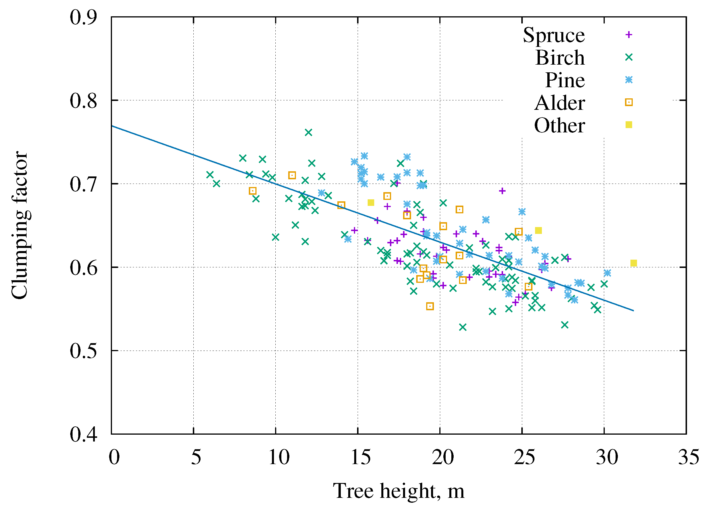
In July 2017, the ALS data were collected over numerous homogeneous forest stands large enough to get robust estimates of tree height, crown length, and clumping parameter value c in Equation (5). Based on the analysis of ALS data by Arumäe and Lang [33], the stand height was determined as the 80% level of hits. The crown length was estimated as the range of the hits height where the distribution density exceeded the level , where . The selection of stands included 84 birch stands with age from 10 to 130 years, 50 pine stands with age from 50 to 195 years, 39 spruce stands with age from 10 to 205 years, 18 common alder stands with age from 10 to 155 years, and three stands of other species. The range of forest heights was from 4 to 32 m, and crown lengths ranged from 3 to 24 m. In most cases, the share of main species in stands was over 50%, and in 70 stands it was over 90%. The site index varied in the range from 12 m to 38 m. The allometric LAI using relations by Marklund [34] and Repola [35] was in the range from 0.3 to 11.2 and from 0.3 to 13.2, respectively. The relation of the clumping parameter c to some stand parameters was close to linear, and correlation coefficients were as high as 0.74 (the absolute value), see Table 2 and Figure 8, Figure 9 and Figure 10. The multiple correlation coefficient of two independent parameters—tree height and crown length—and clumping parameter c was 0.79.
At the same time, the measurements with different ALS instruments in different years returned different values of the clumping parameter. In the RAMI stands, the results were 0.638 and 0.819 in the pine stand, 0.654 and 0.858 in the birch stand, and 0.653 and 0.914 in the spruce stands in 2017 and 2009, respectively. This difference was caused by the lower vertical resolution and the rather large dead zone (3.5 m) behind a hit of the Leica ALS50-II. The percentage of one, two, and three hits of pulses in 2017 and 2009 measurements differed by 0.6, 1.3, and 5.9 times, respectively .
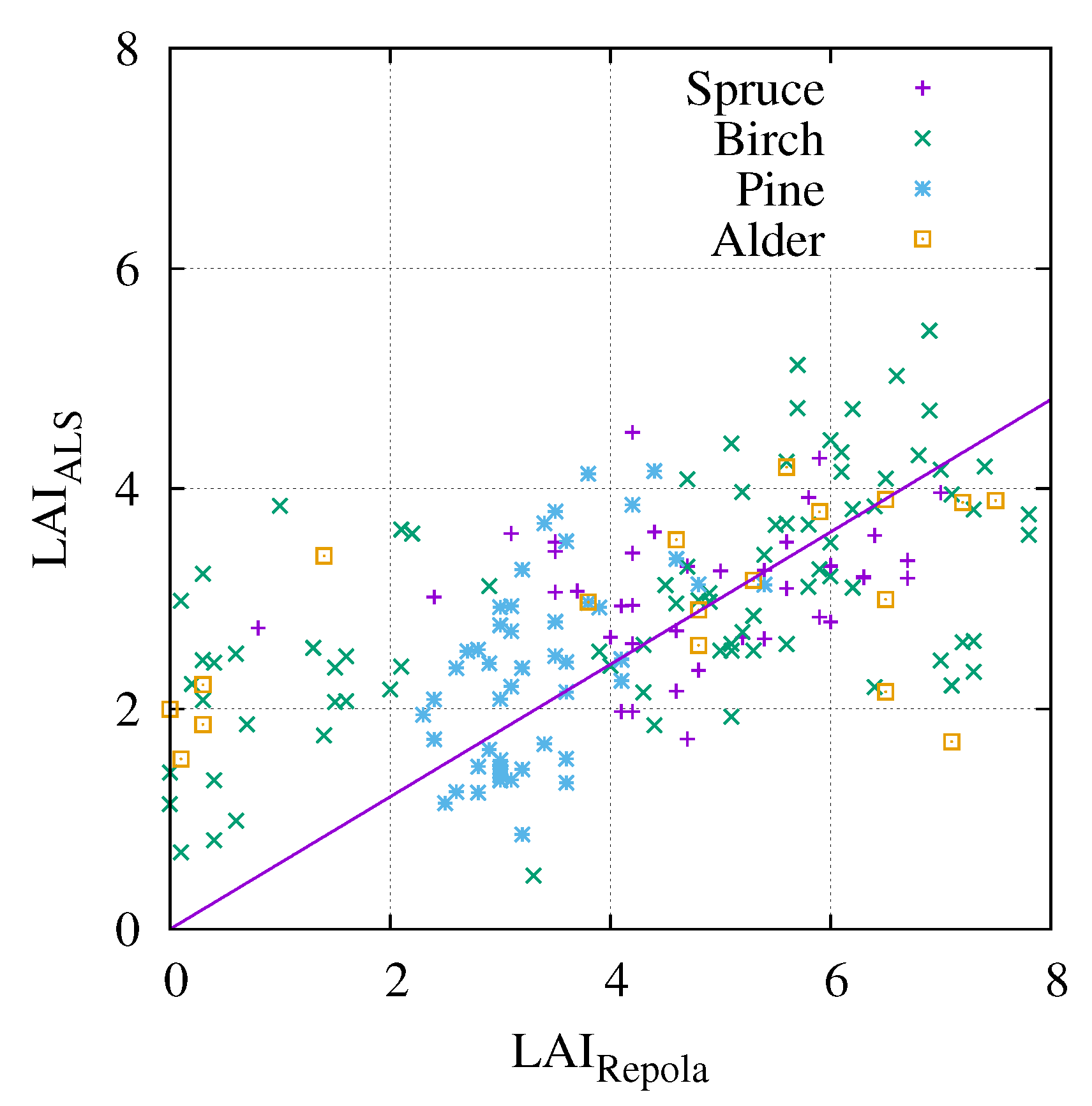
Equation (6) allows the estimation of the plant area index of stands if we know the value of the geometry function . The assumption of spherical orientation may be a rather good approximation for conifer needles and tree leaves, but the BRDF measurements confirm that there was a tendency to the erectophile nature of directional reflectance forming elements in hemi-boreal forests [29]. Therefore, the suggestion by Kuusk [16] for the values was used for the estimation of plant area. Figure 11 and Figure 12 show the correlation of plant area index estimated by Equation (6) and allometric LAI by Marklund [34] and Repola [35], respectively. The values of correlation coefficient were not very high:
= 0.494,
= 0.569.
At the same time, the allometric LAI estimates also differed. Their mutual correlation coefficient was = 0.85 . Allometric LAI estimates used the mensuration data of 2011. Therefore, the allometric LAI values of young stands (low LAI values) were obviously underestimated, and we could expect an even better correlation of allometric and ALS LAI estimates if simultaneous data were used.
4. Discussion
In radiative transfer in a vegetation canopy, transmittance (the gap fraction) has a key role in direct radiation and the chance of a photon to escape. The estimates of the leaf area of forests are also based on the measurements of gap fraction. The large variability of structure and the large height of forests makes the measurement of gap fraction in forests difficult. Indirect optical methods, passive optical methods, and sounding with laser scanners were used for the estimation of gap fraction in forests. It is possible to compare the gap fraction in different forests using only one device and method, but systematic bias may be possible. The comparison of gap fraction estimates in thoroughly studied mature forest stands using different instruments and methods demonstrates how different the estimates could be. While ALS is used for the estimation of gap fraction near zenith and the TRAC instrument allows the estimation of gap fraction only at large zenith angles at hemiboreal latitudes, TLS and hemispherical photos allow the analysis of the whole angular profile of the gap fraction. Compared to HP-s, TLS techniques underestimate gap fraction in forests significantly. Obviously, part of this difference is caused by the overestimation of gap fraction in HP methods if the specular reflection of sky radiation on foliage is ignored. At the same time, there may be problems specific to the TLS techniques. The processing of the laser scanner signal by the proprietary software during measurements may be different in different instruments, and thus the instruments of different providers may give different results [36] —something we could see when comparing the clumping estimates in RAMI stands using ALS data from 2009 and 2017. The strength of the reflected signal depends on a number of factors: the reflection coefficient and surface roughness of the target hit, the incidence angle on the target, the fraction of the sounding pulse cross section covered by the target, etc. Instrument specifications give the beam FWHH-based and/or Gaussian-based width, however the wings of the beam may give a signal which is qualified as a hit as well . This results in the filling of small gaps in the forest canopy, which is a reason for the underestimation of gap fraction in TLS measurements.
Measurements with TLS and hemispherical photos were taken at few points. ALS measurements offer a huge number of independent samples, but measurements were restricted to the small range of zenith angles near zenith where the uncertainty of terrestrial measurements is the largest. Sampling mismatch complicates the comparison of results. The problem of different results with laser scanners by different providers is also present. The additional possible difference between the TLS footprint and a much wider sounding beam creates additional complications in the interpretation of results. Arumäe and Lang [37] compared vertical canopy cover using hemispherical photos and ALS data in 93 dense deciduous broadleaf-dominated hemi-boreal forest stands. The ALS first hits-based estimate of canopy cover was systematically greater than that from HP techniques, and the scattering of results was high. In the present study, we saw the highest values of gap probability from ALS measurements, however the uncertainty of TLS and HP gap fraction was large at zenith .
Gap fraction in a forest canopy is controlled by plant area (LAI), by the orientation of plant elements (), and by the mutual shading of plant elements—the clumping/regularity of elements 3D pattern. All three of these forest canopy characteristics are difficult to measure, and are known to have large uncertainty. The increasing vertical resolution of new ALS instruments and the huge number of tests in ALS measurements allows a more reliable direct estimation of the clumping of foliage in a forest canopy. The proposed method provides the total foliage clumping index, including the effect of non-randomness at all scales (i.e., shoot, branch, and tree). The method is limited by the vertical resolution of discrete returns. Laser scanners of different spatial resolution will give different estimates of clumping. The analysis of correlation between forest mensuration parameters and clumping factor showed that stand clumping increased with increasing stand height and crown length, while the dependence on stand height was stronger. There was also a negative correlation with basal area. The correlation of LAI estimates using the estimated clumping factor and assumed LAD with allometric LAI estimates was not very high. At the same time, different allometric relations gave different LAI estimates. We do not know which of these three LAI estimates is the best. Allometric relations were developed using sample trees and mensuration data (tree height and breast height diameter of trees). Such data are available only in regularly inventoried forest stands. Allometric relations may not be valid for all trees in a stand. Tree LAI varies depending on the tree age, site quality, stand density, etc. All of these dependencies cannot be considered in simple allometric relations, and thus we do not know how reliable the allometric estimates of LAI are in every separate stand. High-resolution ALS measurements offer another method of estimating the clumping of plant material in a forest stand, and thus help to estimate the LAI of the stand independently of the available mensuration data.
5. Conclusions
The directional gap fraction is a very important characteristic of a forest structure and has a key role in the radiative transfer in a forest canopy. The estimation of the amount of foliage in a forest is based on this characteristic, but it is measured with high uncertainty. At some view angles, discrepancies between estimates using different instruments and different methods may reach more than 100%. None of the methods used (hemispherical photos, plant canopy analyzer LAI-2000, Cajanus sighting tube, the TRAC-instrument, terrestrial and airborne laser scanners) can be considered superior for the estimation of gap fraction in forest canopies.
We also suggested a method for estimating total foliage clumping index from airborne laser scanner measurements, including the effect of non-randomness at all scales (i.e., shoot, branch, and tree scales), derived from the basic equation of gap fraction in a vegetation canopy. This method helps to estimate the LAI of a forest stand from gap fraction data independently of the available mensuration data. The precision of the method increased with the increasing spatial resolution of new instruments. The total clumping index of hemi-boreal forest stands was in the range between 0.5 and 0.8, and decreased with increasing stand height and crown length, while its dependence on stand height was stronger.
Author Contributions
Data curation, A.K., M.L. and S.M.; Formal analysis, A.K.; Funding acquisition, J.P.; Investigation, J.P., M.L. and S.M.; Writing—original draft, A.K.; Writing—review & editing, J.P., S.M. and M.L.
Funding
This research received no external funding.
Acknowledgments
This study was funded by the Estonian Research Council, the project “Quantitative remote sensing of vegetation covers, Project SF0180009Bs11 and Grant 7725”. Jan Pisek was supported by the Estonian Research Council grants PUT232, PUT1355 and Mobilitas Pluss MOBERC-11. The TLS data were pre-processed Chair of Geodesy of Tallinn University of Technology within the frames of the Estonian Environmental Technology R&D Programme KESTA, research project ERMAS, AR12052. The ALS measurements were done by Estonian Land Board.
Conflicts of Interest
The authors declare no conflict of interest.
References
- Levy, E.; Madden, E. The point method of pasture analysis. N. Z. J. Agric. Res. 1933, 46, 267–279. [Google Scholar]
- Warren Wilson, J. Inclined point quadrats. New Phytol. 1960, 59, 1–8. [Google Scholar] [CrossRef]
- Warren Wilson, J. Errors resulting from thickness of point quadrats. Aust. J. Bot. 1963, 11, 178–188. [Google Scholar] [CrossRef]
- Li-Cor. LAI-2000 Plant Canopy Analyzer. Technical Information; LI-COR, Inc.: Lincoln, NE, USA, 1989; p. 24. [Google Scholar]
- Leblanc, S.; Chen, J.; Kwong, M. Tracing Radiation and Architecture of Canopies. TRAC Manual Version 2.1.3; Natural Resources Canada: Ottawa, ON, Canada, 2002; p. 25. [Google Scholar]
- Korhonen, L.; Korhonen, T.K.; Rautiainen, M.; Stenberg, P. Estimation of forest canopy cover: A comparison of field measurement techniques. Silva Fennica 2006, 40, 577–588. [Google Scholar] [CrossRef]
- Kuusk, A.; Lang, M.; Kuusk, J. Database of optical and structural data for the validation of forest radiative transfer models. In Light Scattering Reviews; Kokhanovsky, A., Ed.; Springer: Berlin, Germany, 2013; Volume 7, pp. 109–148. [Google Scholar]
- Kuusk, A.; Lang, M.; Kuusk, J.; Lükk, T.; Nilson, T.; Mõttus, M.; Rautiainen, M.; Eenmäe, A. Database of Optical and Structural Data for the Validation of Radiative Transfer Models. Tartu Observatory, 2015; p. 1. Available online: http://scorpion.to.ee/bgf/jarvselja_db/jarvselja_db.pdf (accessed on 13 May 2018).
- Chen, J.; Black, T.; Adams, R. Evaluation of hemispherical photography for determining plant area index and geometry of a forest stand. Agric. For. Meteorol. 1991, 56, 129–144. [Google Scholar] [CrossRef]
- Jonckheere, I.; Nackaerts, K.; Muys, B.; Coppin, P. Assessment of automatic gap fraction estimation of forests from digital hemispherical photography. Agric. For. Meteorol. 2005, 132, 96–114. [Google Scholar] [CrossRef]
- Cescatti, A. Indirect estimates of canopy gap fraction based on the linear conversion of hemispherical photographs: Methodology and comparison with standard thresholding techniques. Agric. For. Meteorol. 2007, 143, 1–12. [Google Scholar] [CrossRef]
- Lang, M.; Kuusk, A.; Mõttus, M.; Rautiainen, M.; Nilson, T. Canopy gap fraction estimation from digital hemispherical images using sky radiance models and a linear conversion method. Agric. For. Meteorol. 2010, 150, 20–29. [Google Scholar] [CrossRef]
- Pisek, J.; Lang, M.; Nilson, T.; Korhonen, L.; Karu, H. Comparison of methods for measuring gap size distribution and canopy nonrandomness at Järvselja RAMI (RAdiation transfer Model Intercomparison) test sites. Agric. For. Meteorol. 2011, 151, 365–377. [Google Scholar] [CrossRef]
- Glatthorn, J.; Beckschäfer, P. Standardizing the protocol for hemispherical photographs: Accuracy assessment of binarization algorithms. PLoS ONE 2014, 9, e111924. [Google Scholar] [CrossRef] [PubMed]
- Woodgate, W.; Jones, S.; Suarez, L.; Hill, M.; Armston, J.; Wilkes, P.; Soto-Berelov, M.; Haywood, A.; Mellor, A. Understanding the variability in ground-based methods for retrieving canopy openness, gap fraction, and leaf area index in diverse forest systems. Agric. For. Meteorol. 2015, 205, 83–95. [Google Scholar] [CrossRef]
- Kuusk, A. Specular reflection in the signal of LAI-2000 plant canopy analyzer. Agric. For. Meteorol. 2016, 221, 242–247. [Google Scholar] [CrossRef]
- Danson, F.; Giacosa, C.; Armitage, R. Two-dimensional forest canopy architecture from terrestrial laser scanning. In Proceedings of the ISPRS Working Group VII/1 Workshop ISPMSRS’07: Physical Measurements and Signatures in Remote Sensing, 12–14 March 2007 Davos, Switzerland; Schaepman, M., Liang, S., Groot, N., Kneubühler, M., Eds.; International Society for Photogrammetry and Remote Sensing (ISPRS): Paris, France, 2007; pp. 1–3. [Google Scholar]
- Danson, F.; Hetherington, D.; Morsdorf, F.; Koetz, B.; Allgöwer, B. Forest canopy gap fraction from terrestrial laser scanning. IEEE Geosci. Remote Sens. Lett. 2007, 4, 157–160. [Google Scholar] [CrossRef] [Green Version]
- Danson, F.; Armitage, R.; Bandugula, V.; Ramirez, F.; Tate, N.; Tansey, K.; Tegzes, T. Terrestrial laser scanners to measure forest canopy gap fraction. In SilviLaser 2008, Proceedings of the 8th International Conference on LiDAR Applications in Forest Assessment and Inventory, 17–19 September 2008, Heriot-Watt University, Edinburgh, UK; Hill, R., Rosette, J., Suárez, J., Eds.; SilviLaser: Edinburgh, UK, 2008; pp. 335–341. [Google Scholar]
- Calders, K.; Verbesselt, J.; Bartholomeus, H.; Herold, M. Applying terrestrial LiDAR to derive gap fraction distribution time series during bud break. In SilviLaser 2011, Proceedings of the 11th International Conference on LiDAR Applications for Assessing Forest Ecosystems, 16–20 October 2011 University of Tasmania, Hobart, Australia; SilviLaser: Edinburgh, UK, 2011; pp. 1–9. [Google Scholar]
- Seidel, D.; Fleck, S.; Leuschner, C. Analyzing forest canopies with ground-based laser scanning: A comparison with hemispherical photography. Agric. For. Meteorol. 2012, 154, 1–8. [Google Scholar] [CrossRef]
- Widlowski, J.L.; Mio, C.; Disney, M.; Adams, J.; Andredakis, I.; Atzberger, C.; Brennan, J.; Busetto, L.; Chelle, M.; Ceccherini, G.; et al. The fourth phase of the radiative transfer model intercomparison (RAMI) exercise: Actual canopy scenarios and conformity testing. Remote Sens. Environ. 2015, 169, 418–437. [Google Scholar] [CrossRef] [Green Version]
- Kuusk, A.; Lang, M.; Nilson, T. Forest test site at Järvselja, Estonia. In Proceedings of the Third Workshop CHRIS/Proba, Frascati, Italy, 21–23 March 2005; pp. 1–7. [Google Scholar]
- AG, L.G. Leica ScanStation C10. The All-in-One Laser Scanner for Any Application; Leica Geosystems AG: Heerbrugg, Switzerland, 2011; p. 2. [Google Scholar]
- RIEGL. RIEGL VQ-1560i Data Sheet; RIEGL Laser Measurement Systems GmbH: Horn, Austria, 2017; p. 10. [Google Scholar]
- Lang, M.; Arumäe, T.; Laarmann, D.; Kiviste, A. Estimation of change in forest height growth. For. Stud. 2017, 67, 5–16. [Google Scholar] [CrossRef]
- Nilson, T. A theoretical analysis of the frequency of gaps in plant stands. Agric. Meteorol. 1971, 8, 25–38. [Google Scholar] [CrossRef]
- Lang, M.; Nilson, T.; Kuusk, A.; Pisek, J.; Korhonen, L.; Uri, V. Digital photography for tracking the phenology of an evergreen conifer stand. Agric. For. Meteorol. 2017, 246, 15–21. [Google Scholar] [CrossRef]
- Kuusk, A.; Kuusk, J.; Lang, M. Modeling directional forest reflectance with the hybrid type forest reflectance model FRT. Remote Sens. Environ. 2014, 149, 196–204. [Google Scholar] [CrossRef]
- Chen, J.; Cihlar, J. Plant canopy gap-size analysis theory for improving optical measurements of leaf-area index. Appl. Opt. 1995, 34, 6211–6222. [Google Scholar] [CrossRef] [PubMed]
- Chen, J.; Liu, J.; Leblanc, S.; Lacaze, R.; Roujean, J.L. Multi-angular optical remote sensing for assessing vegetation structure and carbon absorption. Remote Sens. Environ. 2003, 84, 516–525. [Google Scholar] [CrossRef] [Green Version]
- Kucharik, C.; Norman, J.; Gower, S. Characterization of radiation regimes in nonrandom forest canopies: Theory, measurements, and a simplified modeling approach. Tree Physiol. 1999, 19, 695–706. [Google Scholar] [CrossRef] [PubMed]
- Arumäe, T.; Lang, M. A validation of coarse scale global vegetation height map for biomass estimation in hemiboreal forests in Estonia. Balt. For. 2016, 22, 275–282. [Google Scholar]
- Marklund, L.G. Biomass Functions for Pine, Spruce and Birch in Sweden; Swedish University of Agricultural Sciences: Umeå, Sweden, 1988; p. 73. [Google Scholar]
- Repola, J. Biomass equations for birch in Finland. Silva Fennica 2008, 42, 605–624. [Google Scholar] [CrossRef]
- Keränen, J.; Maltamo, M.; Packalen, P. Effect of flying altitude, scanning angle and scanning mode on the accuracy of ALS based forest inventory. Int. J. Appl. Earth Obs. Geoinf. 2016, 52, 349–360. [Google Scholar] [CrossRef]
- Arumäe, T.; Lang, M. Estimation of canopy cover in dense mixed-species forests using airborne lidar data. Eur. J. Remote Sens. 2018, 51, 132–141. [Google Scholar] [CrossRef]
Figure 1.
Map of the test site. Yellow squares are the RAMI stands, red points are the leaf area index (LAI) points in RAMI stands, empty blue polygons mark the area of airborne laser scanner (ALS) data in 2017, and filled polygons mark the area of ALS data in 2009.
Figure 1.
Map of the test site. Yellow squares are the RAMI stands, red points are the leaf area index (LAI) points in RAMI stands, empty blue polygons mark the area of airborne laser scanner (ALS) data in 2017, and filled polygons mark the area of ALS data in 2009.

Figure 2.
Distribution function of ALS hits in the RAMI pine stand. 1—first hits, 2—all hits, 3—weighted hits, 4—last hits.
Figure 2.
Distribution function of ALS hits in the RAMI pine stand. 1—first hits, 2—all hits, 3—weighted hits, 4—last hits.

Figure 3.
Distribution function of ALS hits in the RAMI pine stand in 2009 and 2017.

Figure 4.
Distribution function of ALS hits in the RAMI birch stand in 2009 and 2017.

Figure 5.
Distribution function of ALS hits in the RAMI spruce stand in 2009 and 2017.

Figure 6.
Gap fraction estimates: (a) pine stand; (b) birch stand; (c) spruce stand. TRAC—TRAC instrument, TLS—terrestrial laser scanner, HSPI—hemispherical images, ALS—airborne laser scanner.
Figure 6.
Gap fraction estimates: (a) pine stand; (b) birch stand; (c) spruce stand. TRAC—TRAC instrument, TLS—terrestrial laser scanner, HSPI—hemispherical images, ALS—airborne laser scanner.

Figure 7.
Dependence of the gap fraction estimate on the thickness of differential layers ; 1—the pine stand, 2—the spruce stand, 3—the birch stand.
Figure 7.
Dependence of the gap fraction estimate on the thickness of differential layers ; 1—the pine stand, 2—the spruce stand, 3—the birch stand.

Figure 8.
Tree height and clumping factor.

Figure 9.
Crown length and clumping factor.

Figure 10.
Basal area and clumping factor.

Figure 11.
Allometric [34] and ALS estimates of LAI.
Figure 11.
Allometric [34] and ALS estimates of LAI.

Figure 12.
Allometric [35] and ALS estimates of LAI.
Figure 12.
Allometric [35] and ALS estimates of LAI.


Table 1.
Description of three forest stands in the Järvselja database [7].
Table 1.
Description of three forest stands in the Järvselja database [7].
| Stand | Age | N | H | LAI | ||
|---|---|---|---|---|---|---|
| Birch | 49 | 992 | 27 | 3.93 | 0.80 | 1.09 |
| Pine | 124 | 1122 | 16 | 1.86 | 0.74 | 0.79 |
| Spruce | 59 | 1689 | 23 | 4.36 | 0.90 | 1.25 |
Age—stand age in years; N—number of trees in the 1 ha stand; H—dominant species height in metres; LAI—allometric leaf area index; —canopy cover; —crown cover.
Table 2.
Correlation of estimated clumping parameter and stand parameters.
| Stand Parameter | ||
|---|---|---|
| Tree height | −0.737 | 0.544 |
| Crown length | −0.571 | 0.326 |
| −0.558 | 0.312 | |
| g1 + g2 | −0.519 | 0.270 |
| −0.588 | 0.346 | |
| −0.445 | 0.198 | |
| Stand age | −0.185 | 0.034 |
—site index, the stand height at age of 100 years; g1, g2—basal area of the dominant and second layer trees; LAI—allometric leaf area index; —the coefficient of determination.
© 2018 by the authors. Licensee MDPI, Basel, Switzerland. This article is an open access article distributed under the terms and conditions of the Creative Commons Attribution (CC BY) license (http://creativecommons.org/licenses/by/4.0/).
Share and Cite
MDPI and ACS Style
Kuusk, A.; Pisek, J.; Lang, M.; Märdla, S. Estimation of Gap Fraction and Foliage Clumping in Forest Canopies. Remote Sens. 2018, 10, 1153. https://doi.org/10.3390/rs10071153
AMA Style
Kuusk A, Pisek J, Lang M, Märdla S. Estimation of Gap Fraction and Foliage Clumping in Forest Canopies. Remote Sensing. 2018; 10(7):1153. https://doi.org/10.3390/rs10071153
Chicago/Turabian StyleKuusk, Andres, Jan Pisek, Mait Lang, and Silja Märdla. 2018. "Estimation of Gap Fraction and Foliage Clumping in Forest Canopies" Remote Sensing 10, no. 7: 1153. https://doi.org/10.3390/rs10071153
Note that from the first issue of 2016, this journal uses article numbers instead of page numbers. See further details here.