Article

Accuracy Assessment of Primary Production Models with and without Photoinhibition Using Ocean-Colour Climate Change Initiative Data in the North East Atlantic Ocean

1
St. Petersburg State University, 199034 St. Petersburg, Russia
2
Plymouth Marine Laboratory, West Hoe, Plymouth PL1 3DH, UK
3
Nansen International Environmental and Remote Sensing Centre, 199034 St. Petersburg, Russia
4
MARE—Marine and Environmental Sciences Centre, Faculdade de Ciências, Universidade de Lisboa, 1749-016 Lisbon, Portugal
*
Author to whom correspondence should be addressed.
Remote Sens. 2018, 10(7), 1116; https://doi.org/10.3390/rs10071116
Submission received: 9 June 2018 / Revised: 8 July 2018 / Accepted: 9 July 2018 / Published: 12 July 2018
(This article belongs to the Special Issue Remote Sensing of Ocean Colour)

Abstract

:
The accuracy of three satellite models of primary production (PP) of varying complexity was assessed against 95 in situ 14C uptake measurements from the North East Atlantic Ocean (NEA). The models were run using the European Space Agency (ESA), Ocean Colour Climate Change Initiative (OC-CCI) version 3.0 data. The objectives of the study were to determine which is the most accurate PP model for the region in different provinces and seasons, what is the accuracy of the models using both high (daily) and low (eight day) temporal resolution OC-CCI data, and whether the performance of the models is improved by implementing a photoinhibition function? The Platt-Sathyendranath primary production model (PPPSM) was the most accurate over all NEA provinces and, specifically, in the Atlantic Arctic province (ARCT) and North Atlantic Drift (NADR) provinces. The implementation of a photoinhibition function in the PPPSM reduced its accuracy, especially at lower range PP. The Vertical Generalized Production Model-VGPM (PPVGPM) tended to over-estimate PP, especially in summer and in the NADR. The accuracy of PPVGPM improved with the implementation of a photoinhibition function in summer. The absorption model of primary production (PPAph), with and without photoinhibition, was the least accurate model for the NEA. Mapped images of each model showed that the PPVGPM was 150% higher in the NADR compared to PPPSM. In the North Atlantic Subtropical Gyre (NAST) province, PPAph was 355% higher than PPPSM, whereas PPVGPM was 215% higher. A sensitivity analysis indicated that chlorophyll-a (Chl a), or the absorption of phytoplankton, at 443 nm (aph (443)) caused the largest error in the estimation of PP, followed by the photosynthetic rate terms and then the irradiance functions used for each model.

Graphical Abstract

1. Introduction

The rate of synthesis of organic matter by marine phytoplankton through the process of photosynthesis determines the energy flow through the trophic chain in the global ocean. This process, known as primary production (PP), not only fuels biological growth and fish productivity, but also regulates carbon uptake and release by the ocean [1]. Since the 1950’s, PP has been determined using radio labelled carbon [2] through in situ or simulated in situ incubations. Though these methods have provided great insight into the variability in PP, the number of measurements available is limited both spatially and temporally. The introduction of rapid fluorescent based and O2/Ar ratio methods using membrane inlet mass spectrometry has increased the number of measurements that can be made over time and space, but still cannot provide synoptic coverage at global, basin, or regional scales. The use of ocean colour remote sensing data has revolutionised our ability to monitor PP at higher temporal and spatial scales than can be provided by in situ techniques [3,4,5,6,7,8]. Over the past two decades, there has therefore been a concerted effort to estimate PP from the satellite ocean colour using models based on the following input parameters: (1) Phytoplankton biomass expressed as Chl a, carbon concentration, or phytoplankton absorption; (2) photo-physiology or photosynthetic rates; and (3) the light field. More than twenty models have been developed that are run solely using remotely sensed data. Some of these models have been validated to ascertain their relative or absolute accuracy [9,10,11,12,13,14].
Historic studies have shown that satellite derived PP accounts for 50 to 80% of the variance in measured PP depending on the input parameters used in the model [6,7,9,15,16]. Many of these historic studies are limited by a lack of in situ data to characterize the spatial, temporal, and vertical variability in photo-physiology that cannot be measured by remotely sensed parameters alone. Some parameters used in the model, including photosynthetic rates, are input as constants or as functions of other physical parameters, and their vertical distribution is assumed to be constant with depth, which can lead to significant errors in model performance [9,10,11,17]. In addition, some models fail in regions with atypical optical and photo-physiological properties [18,19,20] and therefore require a specific regional parameterization.
Early validation studies illustrated that the main cause of the difference between modelled and in situ PP was from parameters that characterize the absorption of light by phytoplankton through Chl a, phytoplankton absorption coefficients, or carbon biomass [21,22,23]. This resulted in an over-estimate of PP in eutrophic waters and an under-estimate in mesotrophic and oligotrophic waters [15]. A series of National Aeronautics and Space Administration (NASA) PP model inter-comparisons were conducted in the 2000’s, firstly by [9], who compared twelve different PP models in nine regions of the world ocean using 89 in situ PP measurements, and found that the difference between satellite and in situ estimates of PP was highly correlated with differences between in satellite and in situ Chl a (See also [24]). Errors in the PP model can be further compounded when other input parameters are derived from Chl a. The second NASA PP inter-comparison [10] illustrated that a four-fold variation of Chl a caused a three-fold variation in PP, whereas variations in photosynthetic active radiation (PAR) and sea surface temperature (SST) had smaller effects on PP. This study also showed however, that deriving photosynthetic rates from temperature alone can cause a significant error in PP. More recently, NASA compared twenty-one PP models in ten regions of the World Ocean using 1156 in situ PP measurements, and showed that the main cause of error in PP models was in coastal, optically complex waters where satellite Chl a can be inaccurate [13]. Further to this, Milutinović and Bertino [25] conducted a comprehensive analysis of the errors associated with the parameters used in one PP model (the Vertical Generalized Production Model - VGPM [6]) and showed that up to 90% of the error is associated with the biomass specific optimum photosynthetic rate (PBopt). The use of regional in situ values of photosynthetic parameters in satellite derived models improves the performance of PP models [26,27,28].
In this paper, we assess the accuracy of one Wavelength-Integrated (WIM) and two Depth-Integrated (DIM) models [29] that are commonly used in the literature, in the North Atlantic. The WIM tested is the Platt and Sathyendranath model (PPPSM) [22], which uses an exponential Photosynthesis-Irradiance (P-I) function based on the absorption of light by the photosystems [30,31]. The most commonly used DIM is VGPM (PPVGPM), which is simple and quick to apply to satellite data. By contrast, we also assess the DIM Absorption Based Model (PPAph) [32,33], which uses the optical absorption signature of phytoplankton as an empirical function of phytoplankton biomass to derive PP. To date, few models include a photoinhibition term that accounts for the photosynthetic rate with increasing irradiance that can occur under high light conditions or when the phytoplankton community moves suddenly from low to high light, which can cause a decrease in the photosynthetic efficiency [34].
Model performance was assessed using 95 in situ measurements of daily water column primary production (PPeu) from the NEA. The models were run using the ESA, OC-CCI version 3.0 data. The paper addresses the following questions: (1) which is the most accurate model for this region? (2) Does the model performance improve when implementing a photoinhibition function? (3) Does the accuracy of each model change depending on the province and season? (4) What is the accuracy of the models using both high (daily) and low (weekly) temporal resolution data? (5) Which input parameter causes the greatest error in each model?

2. Materials and Methods

2.1. Study Region

Stations of PPeu were sampled in the North East Atlantic (20–65° N, 5–40° W) from 1998 to 2013, covering the four biological provinces according to [35]: the ARCT, NADR, NAST, and NATR (North Atlantic Tropical Gyre province) (Figure 1, Table 1). A total of 95 stations were analysed during summer (May–August) and in autumn (September–October). Based on OC-CCI Chl a during the sampling periods, 54% of the stations were in oligotrophic waters (0–0.1 mg m−3) and 42% were mesotrophic (0.1–1 mg m−3) [36].

2.2. Simulated In Situ 14C Primary Production Measurements (PPeu)

PPeu was determined on Atlantic Meridional Transects (AMT) 6, 12, 13, 14, 15, 16, 18, 19, 21, 22, and 23 [37], Ecosystem of the Mid-Atlantic Ridge (ECOMAR) cruises in the North Atlantic JC011 and JC037, and cruise D264 in the Celtic Sea [14]. Water samples were taken from 6 to 9 depths and transferred from Niskin bottles to black carboys to prevent shock to the photosynthetic lamellae of the phytoplankton cells. Water from each sample was sub sampled into three 75 mL clear polycarbonate bottles and three black polycarbonate bottles. The bottles were pre-cleaned following Joint Global Ocean Flux Study (JGOFS) protocols to reduce trace metal contamination [38]. Each sample was inoculated with between 185 and 740 kBq (5–20 µCi) NaH14CO3 according to the biomass of phytoplankton and transferred to an on deck (simulated in situ) incubation system using neutral density and blue filters to simulate subsurface irradiance over depth to 97%, 55%, 33%, 20%, 14%, 1%, or 0.1% of the surface value. Incubations were conducted from dawn to dusk for 10 to 16 h. The upper four light levels were maintained at the in situ temperature by pumping water from the sea surface into the incubators, and the two lower light depths were chilled with fresh water from a water bath maintained at within ±3 °C of the in situ temperature. For all cruises, after incubating the water samples, suspended material was filtered through 0.2 µm polycarbonate filters at a vacuum pressure of <20 cm Hg. The filters were then rinsed with filtered seawater, exposed to concentrated HCl fumes, and immersed in a 5 mL scintillation cocktail. 14C disintegration time per minute (DPM) was measured on board on either a Beckman LS6000 SC or a TriCarb 3900 TR liquid scintillation counter (LSC) using the external standard and the channel ratio methods to correct for quenching. The quantity of 14C added to the experimental bottles was determined by adding aliquots of the stock 14C solution to Carbosorb, a CO2 absorbing scintillation cocktail, and counted immediately on the LSC.

2.3. Satellite Data

To estimate PP, satellite ocean colour, SST, and PAR data were used. Each model was firstly run using daily OC-CCI v.3.0 data. This was then compared using eight day composite OC-CCI data, which is freely available to end-users through the internet. From the OC-CCI database Chl a concentration [mg m−3], the downwelling diffuse attenuation coefficient (kd) at 490 nm [m−1] and the absorption coefficient of phytoplankton (aph) at 443 nm [m−1] were obtained from the merged information of four ocean colour sensors (SeaWiFS, MODIS-Aqua, MERIS, and VIIRS) at a spatial resolution of 4 × 4 km. The data was firstly filtered to exclude possible outliers related to the weather conditions and edge of cloud effects. This was performed by log transforming the data and then screening for outliers, which differed by more than four standard deviations (over 21 × 21 pixels area) from the average at each match-up station. Additional filtering was conducted according to the type of water masses; only Case 1 waters, according to [39], were analysed in the study. All pixels classified as eutrophic based on a euphotic depth of <9.8 m [40], and for Case 2 waters based on kd 490 nm > 0.47 m−1, were removed.
Daily and eight-day PAR (E m−2 day−1) data with a spatial resolution of 4 × 4 km were downloaded from the NASA’s OceanColor Web. Averaged values from two ocean colour sensors, SeaWiFS and MODIS-Aqua, were used. Preliminary analysis showed that the difference between PAR values from two sensors was less than 3%. Therefore, using one sensor only, instead of the average of the two, when another sensor is not available does not cause significant errors.
Daily SST data [°C] with a spatial distribution 1 × 1 km were downloaded from the Multiscale Ultra-high Resolution Sea Surface Temperature database, which is a merged data set from AVHRR, MODIS-Aqua, and AMSR, in which the influence of clouds is reduced due to the use of both infrared and microwave satellite data. As daily SST data have a 1 × 1 km spatial distribution, we re-gridded them to 4 × 4 km, in alignment with the ocean colour data.

2.4. Satellite Models of Primary Production

The models that were assessed in this study are commonly used to estimate PP, but are architecturally different. PPVGPM is forced by ocean colour Chl a and the variability in the photosynthetic rate is parameterized from satellite SST. PPAph is based on the absorption properties of phytoplankton (aph), which can be derived directly from the inversion of remote sensing reflectance rather than from Chl a [41]. The principal advantage of using phytoplankton absorption at 443 nm-aph (443) is that it minimizes the effects of coloured dissolved organic matter and non-algal absorption, which can adversely affect PP models by modifying the light field [41,42]. PPPSM is more complex than the other two models [43], since it simulates changes in photosynthesis as a function of irradiance using a two-parameter exponential P-I function based on the theory of initial light absorption by the photosynthetic system [30,31]. By contrast, PPVGPM and PPAph use the Michaelis-Menten equation [44].
PPVGPM retrieves PPeu. It was parameterized using Chl90 [mg m−3], which is the average Chl a concentration in a layer of the first optical depth seen by ocean colour sensors, zeu, which is the euphotic depth, [m], I0 is the daily surface PAR, [E m−2 day−1], DL is the day length, [h], and an empirical coefficient, 0.66125 (see Equation (1)). PBopt [mg C (mg Chl)−1 h−1], in the VGPM, was retrieved as a function of SST according to the algorithm presented in [6]. The P-I function (given in square brackets) is based on the Michaelis-Menten equation, with the half saturated constant equal to 4.1 E m−2 day−1:
P P e u = C h l 90 z e u 0.66125 [ P o p t B I 0 4.1 + I 0 ] D L ,
PPPSM retrieves daily PP for a specific depth, z, PP(z), based on the P-I function as an exponential curve:
P P ( z ) = C h l ( z ) [ P m B ( 1 exp ( α B I ( z ) P m B ) ) ] D L ,
where, Chl(z) is Chl a at a specific depth, z, (mg m−3) and I(z) is PAR at a depth, z. The P-I function is based on two independent parameters: the biomass specific maximum rate of photosynthesis (PBm) (mg C (mg Chl)−1 h−1) and the initial slope (αB) (mg C (mg Chl)−1 h−1 (μ E m−2 s−1)−1).
For PPAph, daily PP(z) is calculated as follows:
P P ( z ) = a p h 443 × [ ϕ m × K ϕ K ϕ + I ( z ) ] × I ( z ) ,
where aph (443) is the coefficient of light absorption by phytoplankton at 443 nm [m−1]. In Equation (3), the expression in square brackets corresponds to the photosynthesis dependence on underwater illumination expressed in terms of quantum yield (φ), which is the number of molecules of carbon dioxide assimilated by phytoplankton per absorbed light quantum [45]. In PPAph, the φ-I curve is also presented as the Michaelis-Menten equation, where ϕ = P I [46]. For the φ-I curve, φm is the maximum quantum yield of photosynthesis, [mg C E−1], which is observed at low illumination, and Kφ is the half-saturation constant, [E m−2 day−1]. Usually, the value of Kφ is taken equal to 10 E m−2 day−1 [28,32,33,42,47], corresponding to φm = 0.06 mole C E−1. These values of φm and Kφ were obtained based on the analysis of experimental data; the value of φm corresponds to a theoretical maximum [44,48,49].
For PPPSM and PPAph, the photosynthetic parameters were chosen to be as close as possible to those observed in the NEA. In situ values of PBm, αB, and φm were taken during different seasons (spring, summer, and autumn) and at different depths [32,43,50,51,52,53,54,55] as average values and used in the models as constant values (Table 2). For PPAph, Kφ was determined from the φ-I curve for the widespread coastal phytoplankton diatom species, Skeletonema costatum, following [56]. Thus, for a value of φm of 0.032 mole C E−1 (or 347 mg C E−1 used for PPeu retrieval), Kφ is equal to 138.6 μ E m−2 s−1. Since, the φ-I function in PPAph is expressed as daily values, Kφ is between 4.5–8.0 E m−2 day−1 depending on the day length.
To facilitate the comparison of PPPSM, PPAph, and PPVGPM, the P-I functions of PPPSM and PPAph were integrated over the depth of the euphotic layer (presented in Appendix A, Table A1(a). For each model, it was assumed that the rate of photosynthesis does not depend on a wavelength of the electromagnetic spectrum and is constant during a photoperiod. The Beer–Lambert–Bouguer law, as a function of the surface PAR (I0), was used to propagate I(z) over depth, as follows:
I ( z ) = I 0   e x p ( k d z )
where kd is the downwelling diffuse attenuation coefficient of solar radiation in water [m−1]. The euphotic depth was calculated using the following equation, which is derived from Equation (4), assuming that the surface radiation corresponds to 100% and radiation at the euphotic depth is 1%:
z e u   =   l n ( 100 ) k d = 4.6 k d ,
where kd for the whole spectrum of PAR was calculated as a function of the satellite product, kd, at 490 nm according to the algorithm given in [57].

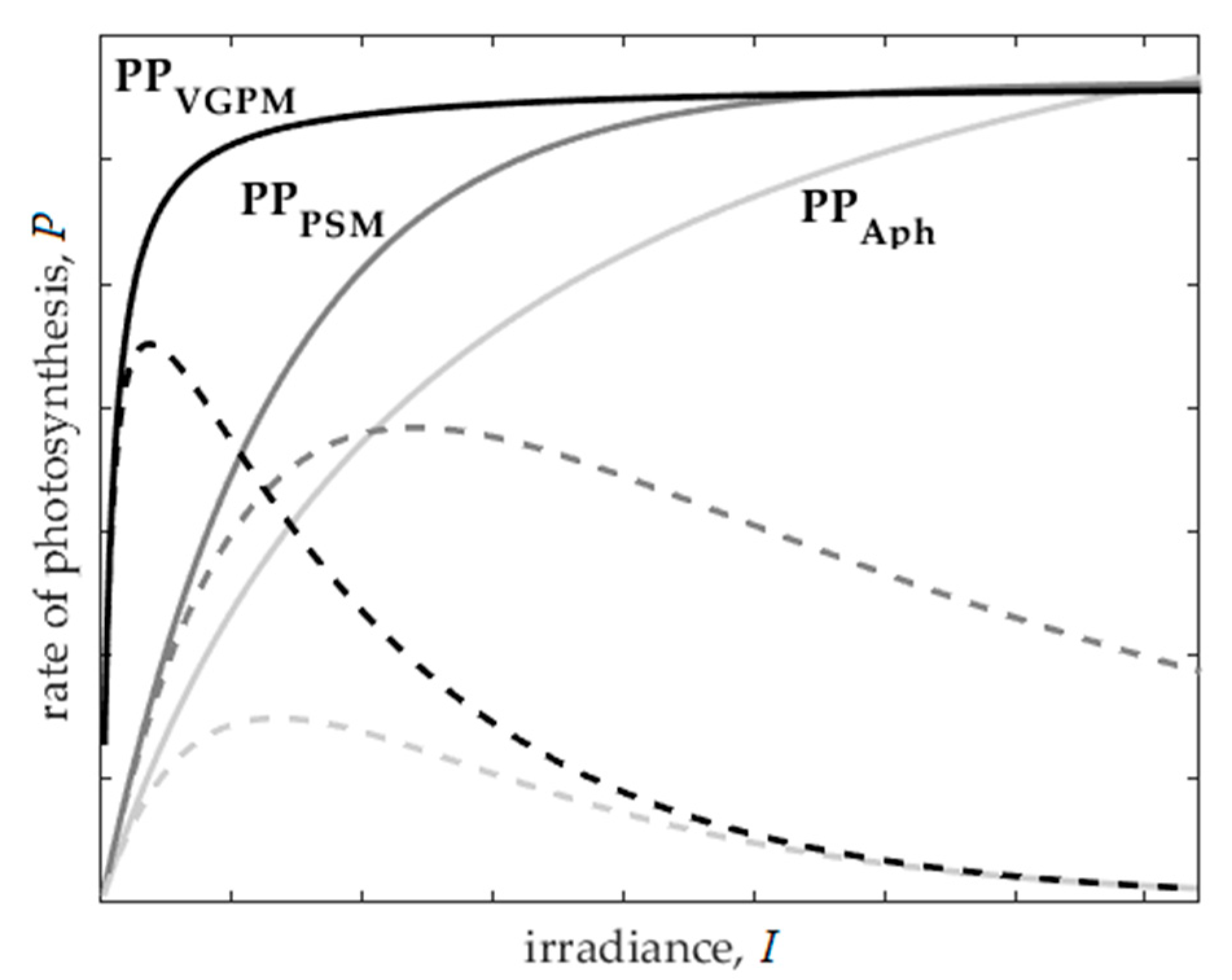
2.5. Implementation of Photoinhibition in the Primary Production Models

PP can be modified by photoinhibition because of phytoplankton being subjected to high irradiance or from moving from low to high light conditions. A photoinhibition function was also implemented for each model to test the significance of this phenomenon in the North Atlantic. The mathematical parametrization of photoinhibition is given in Appendix A, Table A1(b), where βB and β are the photoinhibition parameters, and the superscript, B, represents the photoinhibition normalized to biomass.
PPβPSM uses βB [mg C (mg Chl)−1 h−1 (μ E m−2 s −1)−1], whereas PPβAph uses β [(E m−2 day−1)−1]. Photoinhibition in PPβVGPM is synonymous with the photoinhibition term in PPβAph, where I ¯ is the weighted average irradiance in the water column [E m−2 day−1]. Values of βB = 0.01 mg C (mg Chl)−1 h−1 (μ E m−2 s−1)−1 [43] were used for PPβPSM, and β = 0.01 (E m−2 day−1)−1 [32] for PPβAph and PPβVGPM were used as constants at all stations. Figure 2 shows the P-I functions of the models used. For PPβAph, the φ-I function is multiplied by I.

2.6. Validation Statistics

Satellite derived estimates of PPeu for each 4 × 4 km pixels were compared with ship-borne in situ measurements using the statistics described in [58]. Satellite PPeu data was extracted from 3 × 3 pixels and averaged over the area to compare with in situ point data. For the daily data, only satellite data with a coefficient of variation (CV) of <0.15 over the 3 × 3 pixels were used. Since the OC-CCI data is from the merger of four Ocean Colour sensors (SeaWiFS, MODIS-Aqua, MERIS, and VIIRS), each of these satellites have different over pass times with respect to the in situ data. The Atlantic Meridional Transect field campaigns were designed to match the overpass of these sensors within ±3 h of the different satellite overpasses. Firstly, Taylor [59] and scatter diagrams were used to give the pair correlation (r), Standard Deviation (SD), centre-pattern Root Mean Square Error (c.-p. RMSE), and linear regression (coefficients S and I) between the modelled and in situ PPeu data. For small rows (less than 28 values), the Spearman r was calculated, while for longer ones the Pearson r was used. In addition, the bias, RMSE, and Absolute Percentage Deviation (APD) were calculated. A one-way analysis of variance (ANOVA) was used to assess whether there were significant differences between the model and in situ PPeu means.
Statistics were calculated for all stations in individual provinces and by season except for the ARCT province, which were only available during summer.
For the accuracy assessment, results are only included in Table A3 (Appendix B) when the r between the modelled and in situ PPeu have p-levels of <0.1, 0.05, and 0.01. For all statistics, the highest significant values are highlighted in grey to indicate the most accurate model.

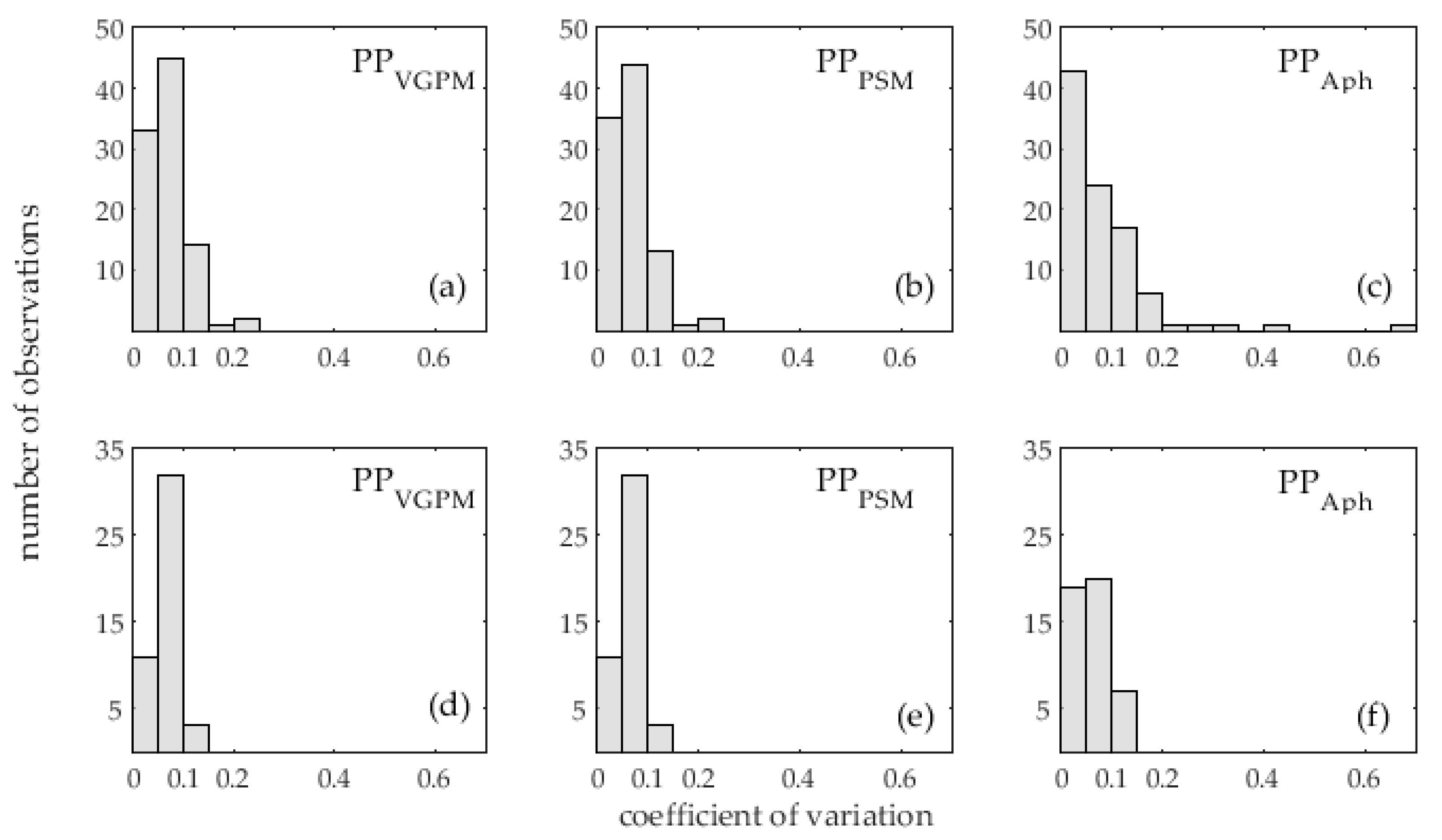
2.7. Sensitivity Analysis

To estimate the contribution of each input parameter to the variability in satellite derived PPeu, a sensitivity analysis was conducted following [14]. The average values of the satellite derived input parameters and the P-I functions were sequentially varied over their natural range.
Firstly, “reference” values of PPeu were calculated based on averaged values of each of the parameters for the three models without photoinhibition. Then, each parameter was varied sequentially, whilst keeping the other parameters fixed at their average value. The results are presented in the form of box-and-whisker diagrams. Since, zeu was estimated by kd (see Equation (5)), it was not included in the sensitivity analysis, but kd was considered instead.
All calculations and visualization of the results were carried out using Matlab R15b.

3. Results

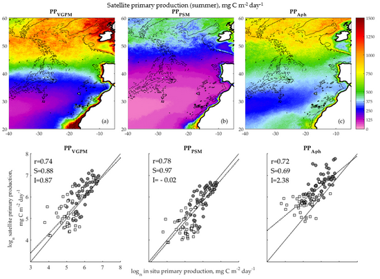
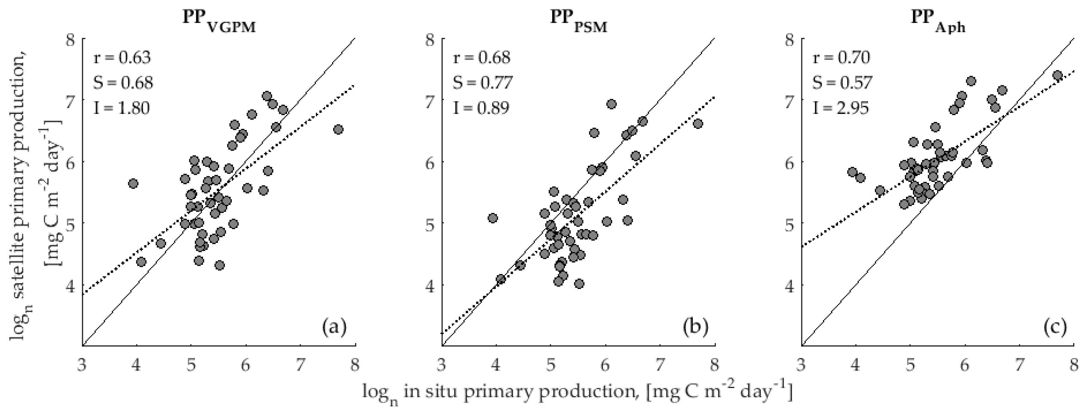
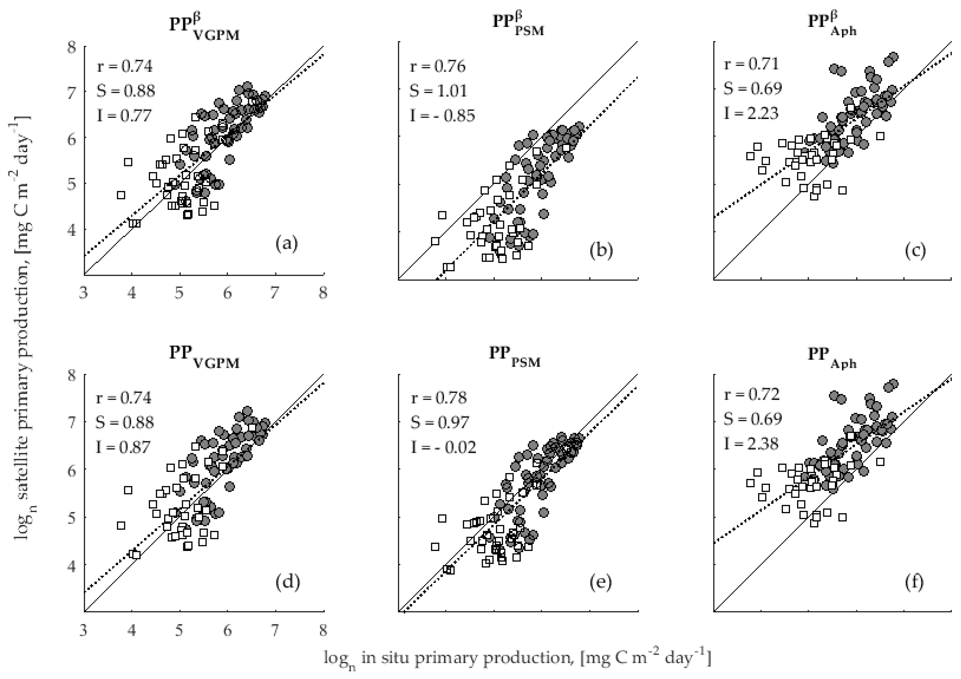
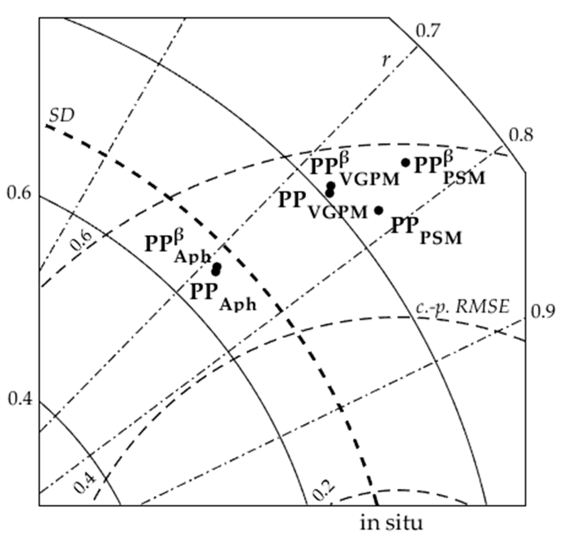
3.1. Accuracy Assessment of Primary Production Models

Each model was firstly run using daily OC-CCI data and compared with in situ PPeu at 46 stations in the NEA (Figure 3). Since the OC-CCI data is available as eight day composites, a secondary accuracy assessment was carried out using these data at the same stations (Appendix B, Table A2) and then including more data (Appendix B, Table A3). Using N = 46, both the daily and eight day modelled data of PPeu have almost identical results.
Using the eight day OC-CCI composite data, PPPSM was the most accurate model over all stations (Figure 4e). When using the photoinhibition model, PPβVGPM tended to over-estimate in situ PPeu at higher values and under-estimate it at lower values (Figure 4a). The net result, however, was that, compared to the other models with photoinhibition, the regression line for PPβVGPM was closest to the 1:1 line and the intercept was the smallest. By comparison, PPβAph tended to over-estimate in situ PPeu, especially at low values, which increased the scatter, resulting in a higher intercept (Figure 4c). For PPβPSM, all points were below the 1:1 line, indicating an under-estimate compared to in situ PPeu (Figure 4b). The scatter was low, however, which increased the percentage variance explained and, though the slope was off set, it was highly correlated with the 1:1. Using no photoinhibition, the trend was the same for PPVGPM and PPAph (Figure 4d,e), with similar statistical results to the models implemented with photoinhibition. For PPPSM, there was a significant improvement in the model prediction of in situ PPeu, with the regression line close to the 1:1 line and the intercept was reduced.
A Taylor diagram was used to illustrate the statistical relationships between modelled and in situ PPeu (Figure 5). All models have a high correlation with in situ PPeu, with r in the segment from 0.7–0.8. The modelled values, however, have a large c.-p. RMSE, though it did not exceed the SD of the in situ measurements. The smallest c.-p. RMSE was for PPAph, PPβAph, and PPPSM. PPPSM had the largest r, but its SD exceeded that of the in situ PPeu, whereas the SD of PPAph and PPβAph were closer to the in situ PPeu SD. Photoinhibition in PPPSM significantly increased the c.-p. RMSE and created a difference in SD compared to the other models.
Table A3 (Appendix B) gives the statistical results between the modelled and in situ PPeu. For all stations, PPPSM was the most accurate in four out of eight statistical tests. It slightly under-estimated PPeu (bias = −0.21) and explained 61% of the variance in in situ measurements (coefficient of determination (r2) = 0.61). There was an 8% Absolute Percentage Difference (APD) between PPPSM and in situ PPeu, and this model also had the smallest RMSE. PPPSM exhibited a better performance in summer when it explained 58% of the variance in in situ PPeu, compared to autumn when it was 25%. In addition, PPPSM did not always accurately capture the spatial variability in in situ PPeu since the SD was 1.5 times higher than the SD of in situ PPeu, except for the ARCT and NADR provinces in summer.
By comparison, PPβVGPM was the most accurate in just two out of eight statistical tests, though it was worse in summer (in five out of eight statistical tests). Both PPβVGPM and PPVGPM slightly over-estimated in situ PPeu (bias = 0.13–0.21) except in the NATR province, where it underestimated in situ values. On average, PPβVGPM and PPVGPM diffed from in situ PPeu by 8% and 9% (APD), respectively. For all stations, r2 for PPβVGPM and PPVGPM explained 54 to 55% of the variance of in situ PPeu. The PPβVGPM and PPVGPM was the most accurate in the NATR province and during summer, and the statistical errors were small.
Both PPβAph and PPAph over-estimated in situ PPeu (bias = 0.51–0.64) compared to the other models, especially at low values (Appendix B, Table A3). APD for PPβAph and PPAph were 11% and 13%, respectively. PPβAph and PPAph, both captured the spatial variability in in situ PPeu for all data, and the SD was similar to that of in situ PPeu. In addition, the c.-p. RMSE for PPβAph and PPAph was small compared to the other models, though they were less accurate in autumn compared to summer.

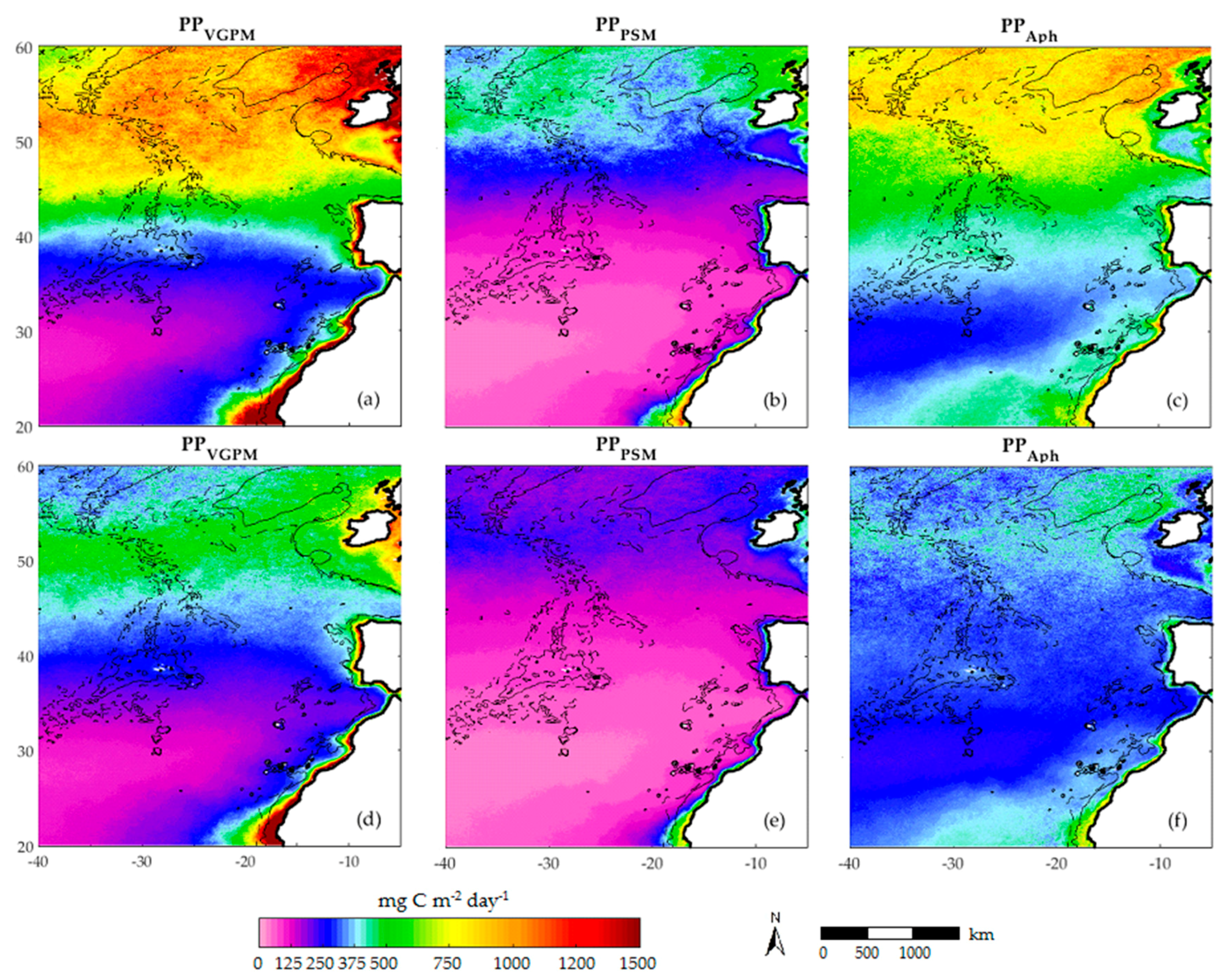
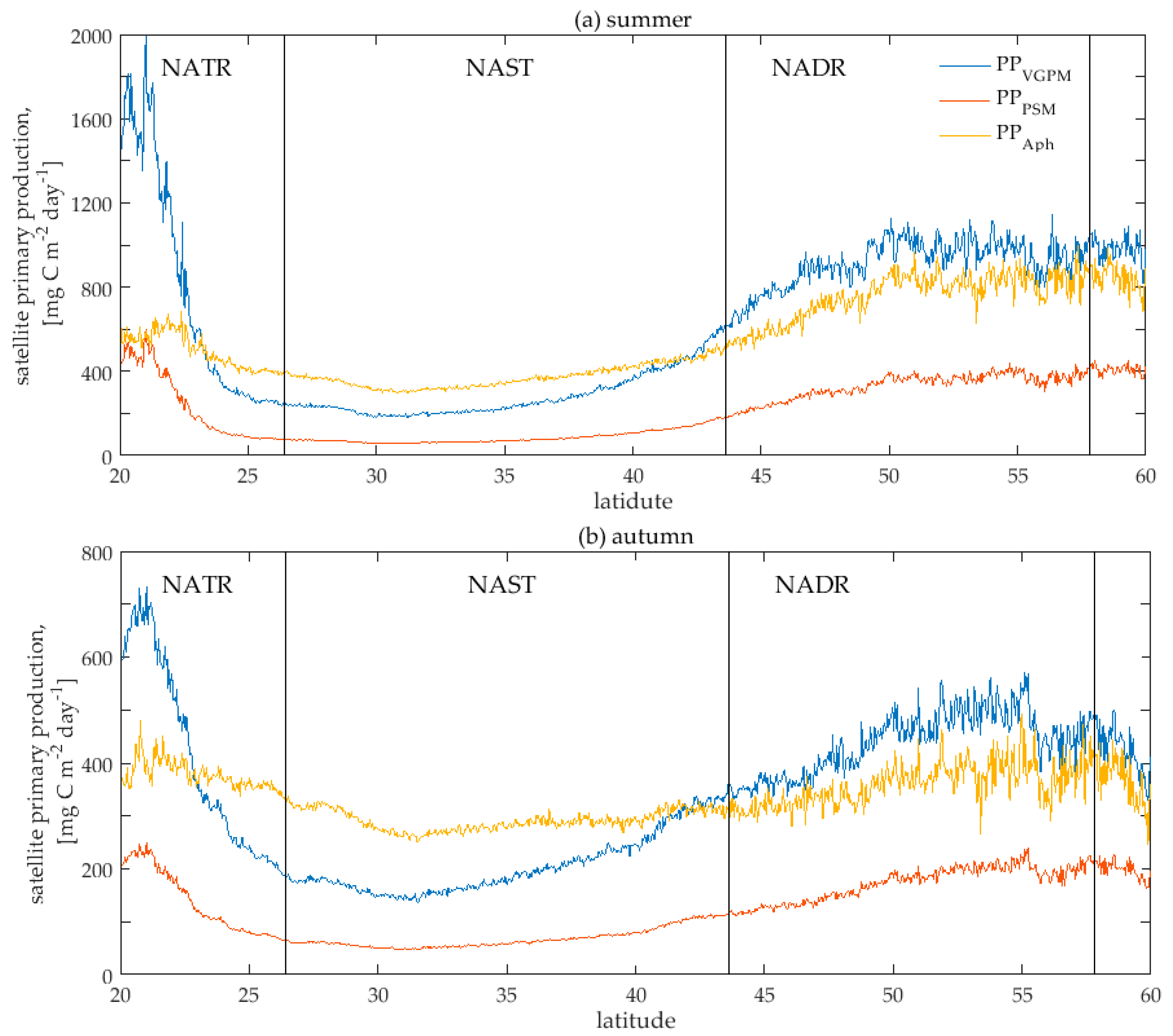
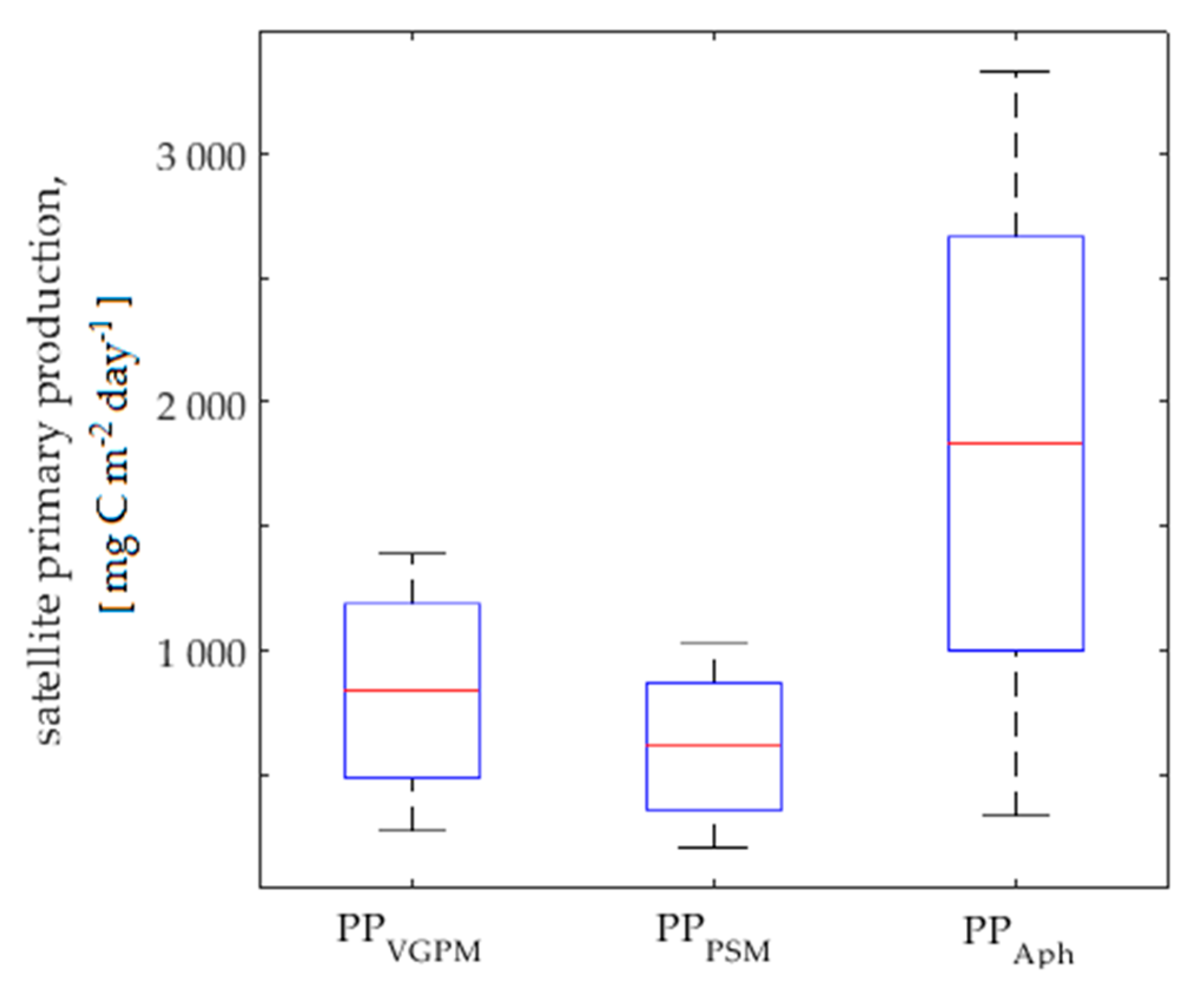
3.2. Satellite Primary Production Images

The spatial and temporal differences between the models are illustrated in satellite images during two different periods: in summer (average June–August, 1998–2011; Figure 6a–c) and autumn (average September–November, 1998–2011; Figure 6d–f). During summer in the NADR, the PPVGPM gave the highest values (500–1500 mg C m−2 d−1), whereas the PPPSM was 250–700 mg C m−2 d−1 and PPAph was 500–1000 mg C m−2 d−1. By comparison, in the NADR autumn, the range in PPVGPM was 300–700 mg C m−2 d−1, PPPSM was 100–300 mg C m−2 d−1, and PPAph was 250–500 mg C m−2 d−1. In contrast, in the NAST in summer, PPAph gave the highest values (250–700 mg C m−2 d−1), which were lower in autumn (200–350 mg C m−2 d−1). The PPVGPM returned similar values in summer and autumn, which were 125–500 mg C m−2 d−1, and PPPSM was 0–350 mg C m−2 d−1. Similarly, in the NATR, PPAph also returned the highest values in both summer and autumn, PPPSM yielded the lowest (<125 mg C m−2 d−1), and PPVGPM were 50–250 mg C m−2 d−1.
To illustrate further the spatial and temporal differences between the models, we extracted data from each model at every 4 km along the transect at 20° W from 20° to 60° N (Figure 7). In the NADR, there was a 182% and 157% Relative Percentage Deviation (RPD) between PPVGPM and PPPSM in summer and autumn, respectively, and 132% and 113% RPD between PPAph and PPPSM, respectively. In the NAST, the differences increased to a 228% and 203% difference between PPVGPM and PPPSM and a 359% and 351% for PPAph and PPPSM in summer and autumn, respectively. For the NATR, there was a 222% and 197% RPD between PPVGPM and PPPSM and a 208% and 224% for PPAph and PPPSM in summer and autumn, respectively.

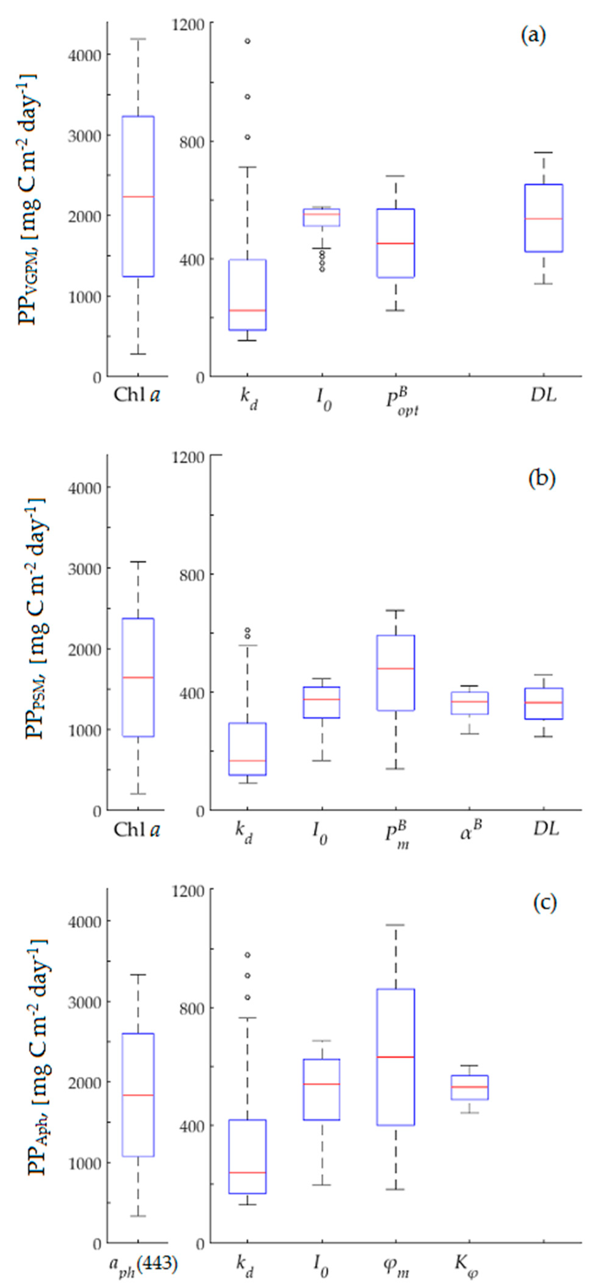
3.3. Model Sensitivity Analysis

For all three models, the largest contribution to the variability in PP was the remote sensing ocean colour product used, which for PPVGPM and PPPSM was Chl a, and for PPAph was aph (443) (Figure 8). The next most important parameter depends on the model used. For PPVGPM, kd for these waters caused the greatest error. For PPPSM, both PBm and kd produced the greatest error and for PPAph it was φm. The third most important parameter for the PPVGPM was PBopt and DL, for PPPSM it was I0 and DL, and for PPAph it was kd and I0. The smallest contribution to the variability in PPVGPM was from I0, but for PPPSM it was αB, and for PPAph it was Kφ.

4. Discussion

4.1. Validation of Primary Production Models

Validation of PPVGPM in the North East Atlantic Ocean has already been carried out by a number of independent studies in this and neighbouring seas [7,9,10,12,13,14,60,61]. These studies report that PPVGPM over-estimates in situ PPeu, which we also observed in the NEA, especially in NADR. The only exception is in the NATR province, where PPVGPM is lower than in situ PPeu. As previously highlighted [7,14], the use of PBopt to simulate model variations in photosynthesis as a function of SST may not consider the displacement of the layer of optimum light conditions for photosynthesis to lower depths, which can be caused by high surface PAR [62].
According to [10], PPVGPM is closer to the actual global PP than PPPSM, which tends to under-estimate global PP by approximately 13%. In our study, PPVGPM are slightly higher than PPPSM in summer and autumn in the Atlantic Ocean, especially in the NADR, NATR, and NAST (Appendix B, Table A3). Only in the ARCT province, where the waters are typically mesotrophic with a medium range Chl a [36], did both models converge.
Validation of PPAph in shelf waters off Argentina [28] showed a high correlation with in situ PPeu (r = 0.9), but there was a tendency for the model to under-estimate PPeu, which is due to the use of the constant, Kφ = 10 E m−2 day−1. In our study, we allowed Kφ to vary between 4.5–8.0 E m−2 day−1 depending on the day length. PPAph slightly overestimated in situ PPeu, especially in autumn, which was also observed by [28] in Argentinian shelf waters.
PPAph in the open ocean waters of the South West Atlantic is also more accurate than PPVGPM ([33]; PPAph r2 = 0.74, PPVGPM r2 = 0.44). Theoretically, this is due to the advantage of deriving aph (443) directly from Rrs rather than using an empirical band ratio to derive Chl a [63]. However, this depends on how accurately both aph (443), aCDOM (443), and adet (443) can be determined from Rrs (443). If there is an error in deriving aCDOM (443) and adet (443) it will propagate to aph (443), which can, in turn, impact PPAph. Based on the sensitivity analysis, aph (443) causes a greater error in PPeu compared to Chl a, which is used in PPPSM (Figure 8). Also for PPAph, an accurate estimate of the photosynthetic parameters (φm and Kφ) is also vital in improving the performance of this model [42]. We also observed that φm has a large impact on PPAph, but Kφ has the least effect (Figure 8). In our study, PPAph was more accurate in the NADR province (r2 = 0.65), though it still over-estimated in situ PPeu and was worse in the ARCT province in summer (Appendix B, Table A3), though this was based on few points. Furthermore, Figure 9 shows that aph (443) causes a significantly greater error in PPAph in the ARCT compared to Chl a used in the PPVGPM and PPPSM.
Standard satellite validation protocols were used to assess the accuracy of the PP models. The satellite data were averaged over 3 × 3 pixels with CV < 0.15 for the majority of the match-ups (Figure 10), which illustrates that the quality of the satellite data was good. For the daily data, the CV for the three models was always <0.15. For the eight day composites, there were two data points for PPVGPM and PPPSM where the CV > 0.15 and six points for PPAph, which were mainly from the ARTC province.
We found that all models performed better in summer than in autumn. Since Chl a is the main contributor to the overall error in modelled PPeu, it may suggest that the error in the autumn values arise from an error in the satellite Chl a. However, numerous studies have shown for the North Atlantic that satellite Chl a is accurate during this season (e.g., [14]).
According to the sensitivity analysis, PBm and φm are the second parameters that determine the overall error of PPeu retrieval. The values of PBm and αB used in the study for the NEA (Table 2) correspond with values from a global database of in situ photosynthesis parameters presented in [64]. Mean values of PBm and αB averaged over four provinces (ARCT, NADR, NAST, and NATR) and over spring, summer, and autumn from this database are 3.25 mg C (mg Ch)−1 h−1 and 0.042 mg C (mg Chl)−1 h−1 (μ E m−2 s−1)−1, respectively. A value of φm = 0.03 mol C E−1 used in our study is characteristic of sunlit regions and was also used by [9] for retrieving PPeu in different parts of the global ocean. An identical value of φm was obtained in waters off the southern California coast (30–34° N) [65]. Errors in PPPSM may arise from inaccurate derivation of the photosynthetic parameters, PBm and αB, which can vary over space, time, and depth depending on the dominant phytoplankton community.
To calculate PPPSM, we used 29 values of PBm, and 20 values during autumn. When a PBm value, typical for autumn, of 2.36 mg C (mg Ch)−1 h−1 was used, it did not improve the correlation between in situ and modelled PPeu (r2 = 0.23). Spatial changes in the species composition of phytoplankton communities and the related changes in photosynthetic rates may also cause a weak correlation between the modelled and in situ PPeu [66]. In addition, we input the Chl a and photosynthetic parameters as constant values over depth, which may not be representative of the vertical variability of these parameters in autumn and may therefore contribute to the error in the model. Kahru et al. [42] validated the PPAph algorithm in the California Current, and showed that accounting for the vertical profile of aph (443) within the euphotic zone improved the correlation between PPAph and in situ PPeu. The coefficient of determination (r2) increased from 0.28 to 0.56. Errors in Rrs, which is used to calculate aph (443), could be the main cause of error in the retrieval of PPeu. These estimates can vary widely between radiometers (15–18% for Rrs at 443 nm).
The tendency in the scatter plots is that PPVGPM over-estimates PPeu in summer and under- and over-estimates PPeu in autumn, PPAph over-estimates PPeu in summer, especially in autumn, and that PPPSM shows good agreement in summer, but has a tendency to under-estimate PPeu in autumn (Figure 4). Visual examination of the resulting mapped images provides a qualitative analysis of whether the tendencies shown in the scatter plots correspond over wider spatial and temporal scales. The extent of the differences between the models in the mapped images and data extracted from these over a transect from 20 to 60° N illustrate that, of the three models, PPVGPM gives the highest PPeu in summer and autumn in the NATR and NADR, whereas the PPAph has the highest PPeu in the NAST, especially in autumn (Figure 7). The PPPSM consistently has the lowest PPeu, but is closest to the in situ PPeu, but the differences between PPPSM and the other models are less in autumn. The outliers in the scatter plot for the PPAph model (Figure 4f) may suggest that, in the higher PP waters of the NADR, this model would return the highest PPeu. The images and transect, however, show that PPVGPM gives the highest PPeu, which is not reflected in the corresponding scatter plot (Figure 4d). The tendency for the PPVGPM to over-estimate PPeu at higher values in the scatter plot represents large areas of the NADR and NATR during summer in the corresponding mapped image (Figure 6a).
The results suggest that the PPPSM model with the OC-CCI data is accurate for the NEA. The model is available as an OC-CCI product, but requires further testing to assess its accuracy over other basins and the entire global ocean.

4.2. Effect of Photoinhibition in Primary Production Models

Photoinhibition describes the decrease in the photosynthetic rate with increasing irradiance [67]. This phenomenon is dependent on the phytoplankton community and its adaptation to the light conditions in the water column. It is usually greatest when phytoplankton is confined to surface high light conditions or when it moves quickly from low to high light [34]. Under such high light conditions, photorespiration can be activated, which is accompanied by utilization of assimilated carbon and, therefore, a decrease in the efficiency of photosynthesis [68]. For different phytoplankton communities, it has been shown experimentally that this effect varies as a function of depth and solar radiation at the surface and photo-adaptation of phytoplankton [69,70]. For example, shade-adapted communities saturate quickly and reach photoinhibition faster than high-light adapted communities.
Since the total amount of incoming solar radiation decreases with the distance from the equator and is dependent on the time of the year, the difference in the estimates of PPeu, both with and without photoinhibition, also decrease with increasing latitude, and has a distinctive seasonal variation associated with the variability of incoming solar radiation during the year. The maximum difference in the estimates of PPeu is in the second half of June, when solar radiation is at a maximum. The smallest difference is at the end of December or beginning of January, when solar radiation reaches a minimum. Since both states can occur in the tropical waters of the NAST and NATR provinces where weak wind stress and density gradient can prevent the migration of the phytoplankton community and, trap it at high light conditions for a significant proportion of the day, including photoinhibition may improve model performance. We found that the PPβVGPM, for example, performed better in the NAST during summer.
Table 3 illustrates the mathematical representation of photoinhibition in the models used, which does not differ significantly between each model. Photoinhibition had a greater effect on PPPSM compared to the other two models, however. Usually, photoinhibition in the models is presented as an exponentially decreasing term [70]. Photoinhibition in PPβPSM is implemented as the P-I curve increases at low light [43]. After integration over the euphotic depth, its mathematical representation can cause large differences between PPβVGPM and PPβAph, even though the photoinhibition functions are identical. According to [32], the photoinhibition term in PPβAph can reduce the values of the modelled PPeu from 10% to 55% depending on the light intensity.

5. Conclusions

Three satellite models of PP were processed using OC-CCI data, with and without photoinhibition, and compared against ship-borne in situ 14C measurements from the NEA. Validation of the models using daily OC-CCI data (N = 46) showed that the PPPSM and PPVGPM had a similar accuracy, whereas the PPAph was not suitable for the region. Using eight day OC-CCI composite data, the number of match-ups was doubled (N = 95) and PPPSM was more accurate over all provinces. For individual provinces, the PPPSM was more accurate in the ARCT and NADR regions whereas the PPVGPM was more accurate in the NAST and NATR regions. The PPAph was the least accurate model for the NEA, which was due to errors in the aph (443) OC-CCI product. The use of a photoinhibition function in the PPVGPM and PPAph had little effect on the model performance, whereas, in the PPPSM, photoinhibition reduced the accuracy of the model, especially at lower range of the values. The performance of the models also varied seasonally; all models were more accurate during summer and less accurate during autumn. Over all provinces, the PPVGPM with photoinhibition was the most accurate during summer, and the PPPSM with no photoinhibition was more accurate during autumn. Mapped images illustrated that differences between models were far greater than indicated by the scatter plots, especially for PPAph and PPVGPM in the NATR and NADR provinces. A sensitivity analysis indicated that the primary ocean colour product (Chl a for PPPSM and PPVGPM; aph (443) for PPAph) caused the greatest variability in model performance, followed by the photosynthetic terms, PBm and φm, in the PPPSM and PPAph models, respectively, and PBopt and kd in the PPVGPM. Improvement in the accuracy of these input parameters will ultimately lead to an improvement in satellite PP algorithms for this region.

Author Contributions

Conceptualization was derived by P.L., I.B. and V.B.; methodology was derived and implemented by P.L. and G.T.; software was developed by P.L. and I.B.; validation was performed by P.L. and G.T.; formal analysis was conducted by P.L. and G.T.; investigation was performed by P.L., G.T., I.B. and V.B.; resources to support the research were provided by P.L., G.T. and I.B.; writing—original draft preparation was done by P.L. and G.T.; writing—review & editing, was done by P.L., G.T., I.B. and V.B.; visualization (data, tables, & figures) was done by P.L.; supervision was from I.B., G.T. and V.B.; project administration was from P.L.; funding acquisition to support the research were sought by P.L. and I.B.

Funding

This work was supported by the Russian Foundation for Basic Research (RFBR grants 18-35-00543 and 16-05-00452), the INTERREG Atlantic Area Cross-border Cooperation Programme project “Innovation in the Framework of the Atlantic Deep Ocean” (iFADO under contract EAPA-165/2016), the UK Natural Environment Research Council National Capability funding for the Atlantic Meridional Transect (AMT) to Plymouth Marine Laboratory.

Acknowledgments

This study was also supported by near real time satellite service from the National Earth Observation Data Archive and Analysis Service (NEODAAS) for the AMT. Acknowledgements are also due to PEst-OE/MAR/UI0199/2014. This is contribution number 328 of the AMT programme.

Conflicts of Interest

The authors declare no conflict of interest. The funders had no role in the design of the study; in the collection, analyses, or interpretation of data; in the writing of the manuscript, and in the decision to publish the results.

Appendix A

Table A1. Mathematical equations for PPPSM and PPAph after integrating their P-I functions over the euphotic depth; (a) E1 is an exponential integral defined as: E 1 ( x ) = x e t t d t ; (b) mathematical representation of photoinhibition in the models tested.
(a) Mathematical Equations for the Models
Model
PPβPSM P P e u = C h l 90 × D L × P m B k d [ ( E 1 ( I 0 β B P m B e x p ( k d z e u ) ) E 1 ( I 0 β B P m B ) ) ( E 1 ( I 0 ( α B + β B ) P m B e x p ( k d z e u ) ) E 1 ( I 0 ( α B + β B ) P m B ) ) ]
PPPSM P P e u = C h l 90 × D L × P m B k d × [ E 1 ( α B × I 0 P m B ) + ( k d × z e u ) E 1 ( α B × I 0 P m B × e x p ( k d × z e u ) ) ]
PPβAph P P e u = a p h 443 × ϕ m × K ϕ k d × e x p ( β K ϕ ) × × [ E 1 ( β ( K ϕ + I 0 e x p ( k d z e u ) ) ) E 1 ( β ( K ϕ + I 0 ) ) ]
PPAph P P e u = a p h 443 × ϕ m × K ϕ k d × [ ln ( K ϕ + I 0 ) ln ( K ϕ + I 0 × exp ( k d × z e u ) ) ]
(b) Mathematical Representation of Photoinhibition
ModelPhotoinhibition TermReference
PPPSM e x p ( β B P m B I ( z ) ) [43]
PPAph e x p ( β × I ( z ) ) [32]
PPVGPM e x p ( β × I ¯ ) I ¯ = 0 z e u I ( z ) d z z e u = 0.215 I 0 this paper

Appendix B

Table A2. Validation statistics for each model using (a) daily and (b) eight day composite OC-CCI data (N = 46). The numbers at the head of the table indicate statistics for one test. The most significant statistical values are highlighted in grey. r is the Pearson pair correlation coefficient, S is the Slope and I is the Intercept of the linear regression coefficients, RMSE is the Root Mean Square Error, and APD is the Absolute Percentage Deviation.
(a) Daily, N = 46123456
rp-LevelCentre-Pattern RMSESIBiasRMSEAPD, %
PPβVGPM0.63p < 0.0010.600.681.73−0.040.609.2
PPVGPM0.63p < 0.0010.600.681.800.050.619.3
PPβPSM0.69p < 0.0010.570.790.16−0.991.1518.8
PPPSM0.68p < 0.0010.570.770.89−0.380.689.9
PPβAph0.71p < 0.0010.480.562.860.420.639.8
PPAph0.70p < 0.0010.480.572.950.560.7411.8
(b) Eight day composites, N = 46
PPβVGPM0.65p < 0.0010.560.661.80−0.060.578.6
PPVGPM0.66p < 0.0010.560.671.860.030.568.6
PPβPSM0.69p < 0.0010.570.790.16−0.991.1518.8
PPPSM0.73p < 0.0010.490.750.98−0.400.649.5
PPβAph0.75p < 0.0010.450.533.000.400.609.4
PPAph0.73p < 0.0010.460.543.090.530.7011.4
Table A3. Validation statistics for each model for the whole region and for individual biogeographical provinces using eight day composite OC-CCI data. The numbers at the head of the table indicate statistics for one test. The most significant statistical values are highlighted in grey. r is the Pearson or Spearman pair correlation coefficient (For N > 28, Pearson was used; for N < 28 Spearman was used, but r2 was not computed), r2 is the coefficient of determination, SD is the Standard Deviation, RMSE is the Root Mean Square Error, S is the Slope, I is the Intercept of the linear regression coefficients, APD is the Absolute Percentage Deviation, and F and p are ANOVA (Analysis of variance) coefficients. Those models, for which the significance of r was more than 0.1, were not included into the analysis and are not presented in the Table for summer stations in NAST (N = 16) and ARCT (N = 12), autumn stations in NADR (N = 6) and NAST (N = 24).
All Stations, N = 9512345678
SDrr2SIbiasRMSECentre-Pattern RMSEAPD, %ANOVA, FANOVA, p
In situ PPeu0.68
PPβVGPM0.810.740.540.880.770.130.570.5691.40.237
PPVGPM0.810.740.550.880.870.210.590.5593.90.051
PPβPSM0.900.760.581.01−0.85−0.780.970.581545.60.000
PPPSM0.840.780.610.97−0.02−0.210.560.5283.60.060
PPβAph0.660.710.510.692.230.510.710.501127.00.000
PPAph0.650.720.520.692.380.640.810.501344.20.000
NADR, N = 28
In situ PPeu0.54
PPβVGPM0.350.730.530.473.700.480.610.38915.10.000
PPVGPM0.350.740.540.483.690.550.660.371019.50.000
PPβPSM0.430.790.620.621.91−0.400.520.3479.10.004
PPPSM0.430.820.670.642.250.100.330.3250.50.468
PPβAph0.370.800.630.543.180.410.530.34810.40.002
PPAph0.380.800.650.563.180.520.620.33916.70.000
NAST, N = 40
In situ PPeu0.57
PPβVGPM0.550.520.270.512.590.070.550.5590.320.572
PPVGPM0.560.540.290.532.570.170.570.54101.680.199
PPβPSM0.490.510.260.441.88−0.971.100.521965.160.000
PPPSM0.500.550.300.482.29−0.340.610.51107.760.008
PPβAph0.420.420.170.314.060.550.780.551423.800.000
PPAph0.440.430.190.344.060.700.890.551636.570.000
NATR, N = 14
In situ PPeu0.33
PPβVGPM0.660.51 1.49−3.22−0.490.680.46115.780.024
PPVGPM0.660.51 1.49−3.13−0.390.610.47103.580.069
PPβPSM0.620.57 1.44−3.89−1.441.500.422654.110.000
PPPSM0.630.54 1.44−3.22−0.770.880.431415.140.001
All Summer Stations, N = 56
In situ PPeu0.49
PPβVGPM0.680.730.541.010.070.140.480.4671.50.218
PPVGPM0.660.730.530.980.350.230.510.4574.30.041
PPβPSM0.800.760.581.25−2.20−0.740.910.541333.90.000
PPPSM0.720.760.581.11−0.84−0.170.500.4772.10.146
PPβAph0.550.670.450.761.940.500.660.43924.90.000
PPAph0.530.660.440.722.320.640.770.421143.00.000
ARCT, N = 12
In situ PPeu0.40
PPβPSM0.280.56 0.453.01−0.370.470.3076.30.020
PPPSM0.280.55 0.463.370.090.310.3040.40.547
NADR, N = 22
In situ PPeu0.39
PPβVGPM0.300.57 0.404.090.390.520.34713.30.001
PPVGPM0.290.55 0.404.220.460.580.34818.90.000
PPβPSM0.340.53 0.532.45−0.470.570.33816.90.000
PPPSM0.320.59 0.503.140.050.320.3150.20.669
PPβAph0.280.58 0.463.680.330.450.3069.70.003
PPAph0.280.62 0.453.880.450.540.30818.60.000
NATR, N = 6
In situ PPeu0.19
PPβVGPM0.210.81 0.800.57−0.500.520.15915.40.003
PPVGPM0.210.81 0.760.93−0.390.420.1679.20.012
All Autumn Stations, N = 38
In situ PPeu0.55
PPβVGPM0.680.410.160.502.640.100.690.68120.50.477
PPVGPM0.670.410.170.502.700.180.690.67121.60.213
PPβPSM0.650.470.220.541.42−0.871.070.621838.60.000
PPPSM0.610.500.250.551.97−0.280.650.58114.40.039
NATR, N = 8
In situ PPeu0.38
PPβVGPM0.840.69 1.67−4.29−0.480.770.60121.90.190
PPVGPM0.850.69 1.69−4.29−0.390.720.60121.20.286
PPβPSM0.770.64 1.53−4.38−1.381.480.532518.00.001
PPPSM0.780.69 1.58−4.00−0.720.900.54134.80.046

References

  1. Falkowski, P. Ocean productivity from space. Nature 1988, 335, 205. [Google Scholar] [CrossRef]
  2. Steemann Nielsen, E. The use of radio-active carbon (C14) for measuring organic production in the sea. ICES J. Mar. Sci. 1952, 18, 117–140. [Google Scholar] [CrossRef]
  3. Smith, R.C.; Eppley, R.W.; Baker, K.S. Correlation of primary production as measured aboard ship in southern California coastal waters and as estimated from satellite chlorophyll images. Mar. Biol. 1982, 66, 281–288. [Google Scholar] [CrossRef]
  4. Eppley, R.W.; Stewart, E.; Abbott, M.R.; Owen, R.W. Estimating ocean production from satellite-derived chlorophyll: Insights from the Eastropac data set. Oceanol. Acta Spec. Issue 1987, SP, 109–113. [Google Scholar]
  5. Antoine, D.; André, J.M.; Morel, A. Oceanic primary production: 2. Estimation at global scale from satellite (coastal zone color scanner) chlorophyll. Glob. Biogeochem. Cycles 1996, 10, 57–69. [Google Scholar] [CrossRef]
  6. Behrenfeld, M.J.; Falkowski, P.G. Photosynthetic rates derived from satellite-based chlorophyll concentration. Limnol. Oceanogr. 1997, 42, 1–20. [Google Scholar] [CrossRef] [Green Version]
  7. Tilstone, G.; Smyth, T.; Poulton, A.; Hutson, R. Measured and remotely sensed estimates of primary production in the Atlantic Ocean from 1998 to 2005. Deep Sea Res. Part II Top. Stud. Oceanogr. 2009, 56, 918–930. [Google Scholar] [CrossRef]
  8. Joo, H.; Son, S.; Park, J.W.; Kang, J.J.; Jeong, J.Y.; Lee, C.I.; Kang, C.K.; Lee, S.H. Long-Term pattern of primary productivity in the East/Japan sea based on ocean color data derived from MODIS-Aqua. Remote Sens. 2016, 8, 25. [Google Scholar] [CrossRef]
  9. Campbell, J.; Antoine, D.; Armstrong, R.; Arrigo, K.; Balch, W.; Barber, R.; Behrenfeld, M.; Bidigare, R.; Bishop, J.; Carr, M.-E.; et al. Comparison of algorithms for estimating ocean primary production from surface chlorophyll, temperature, and irradiance. Glob. Biogeochem. Cycles 2002, 16. [Google Scholar] [CrossRef]
  10. Carr, M.E.; Friedrichs, M.A.; Schmeltz, M.; Aita, M.N.; Antoine, D.; Arrigo, K.R.; Asanuma, I.; Aumont, O.; Barber, R.; Behrenfeld, M.; et al. A comparison of global estimates of marine primary production from ocean color. Deep Sea Res. Part II Top. Stud. Oceanogr. 2006, 53, 741–770. [Google Scholar] [CrossRef] [Green Version]
  11. Friedrichs, M.A.; Carr, M.E.; Barber, R.T.; Scardi, M.; Antoine, D.; Armstrong, R.A.; Asanuma, I.; Behrenfeld, M.J.; Buitenhuis, E.T.; Chai, F.; et al. Assessing the uncertainties of model estimates of primary productivity in the tropical Pacific Ocean. J. Mar. Syst. 2009, 76, 113–133. [Google Scholar] [CrossRef] [Green Version]
  12. Saba, V.S.; Friedrichs, M.A.M.; Carr, M.-E.; Antoine, D.; Armstrong, R.A.; Asanuma, I.; Aumont, O.; Bates, N.R.; Behrenfeld, M.J.; Bennington, V.; et al. Challenges of modeling depth-integrated marine primary productivity over multiple decades: A case study at BATS and HOT. Glob. Biogeochem. Cycles 2010, 24. [Google Scholar] [CrossRef] [Green Version]
  13. Saba, V.S.; Friedrichs, M.A.M.; Antoine, D.; Armstrong, R.A.; Asanuma, I.; Behrenfeld, M.J.; Ciotti, A.M.; Dowell, M.; Hoepffner, N.; Hyde, K.J.W.; et al. An evaluation of ocean color model estimates of marine primary productivity in coastal and pelagic regions across the globe. Biogeosciences 2011, 8, 489–503. [Google Scholar] [CrossRef] [Green Version]
  14. Tilstone, G.H.; Taylor, B.H.; Blondeau-Patissier, D.; Powell, T.; Groom, S.B.; Rees, A.P.; Lucas, M.I. Comparison of new and primary production models using SeaWiFS data in contrasting hydrographic zones of the northern North Atlantic. Remote Sens. Environ. 2015, 156, 473–489. [Google Scholar] [CrossRef]
  15. Balch, W.; Evans, R.; Brown, J.; Feldman, G.; McClain, C.; Esaias, W. The remote sensing of ocean primary productivity: Use of a new data compilation to test satellite algorithms. J. Geophys. Res. Oceans 1992, 97, 2279–2293. [Google Scholar] [CrossRef]
  16. Berthon, J.F.; Morel, A. Validation of a spectral light-photosynthesis model and use of the model in conjunction with remotely sensed pigment observations. Limnol. Oceanogr. 1992, 37, 781–796. [Google Scholar] [CrossRef] [Green Version]
  17. Petrenko, D.; Pozdnyakov, D.; Johannessen, J.; Counillon, F.; Sychov, V. Satellite-derived multi-year trend in primary production in the Arctic Ocean. Int. J. Remote Sens. 2013, 34, 3903–3937. [Google Scholar] [CrossRef]
  18. Dierssen, H.M.; Smith, R.C. Bio-optical properties and remote sensing ocean color algorithms for Antarctic Peninsula waters. J. Geophys. Res. Oceans 2000, 105, 26301–26312. [Google Scholar] [CrossRef] [Green Version]
  19. IOCCG. Remote Sensing of Ocean Colour in Coastal, and Other Optically-Complex Waters; Sathyendranath, S., Ed.; Reports of the International Ocean-Colour Coordinating; IOCCG: Dartmouth, NS, Canada, 2000. [Google Scholar]
  20. Volpe, G.; Santoleri, R.; Vellucci, V.; d’Alcalà, M.R.; Marullo, S.; d’Ortenzio, F. The colour of the Mediterranean Sea: Global versus regional bio-optical algorithms evaluation and implication for satellite chlorophyll estimates. Remote Sens. Environ. 2007, 107, 625–638. [Google Scholar] [CrossRef]
  21. Campbell, J.W.; O’Reilly, J.E. Role of satellites in estimating primary productivity on the northwest Atlantic continental shelf. Cont. Shelf Res. 1988, 8, 179–204. [Google Scholar] [CrossRef]
  22. Platt, T.; Sathyendranath, S. Oceanic primary production: Estimation by remote sensing at local and regional scales. Science 1988, 241, 1613–1620. [Google Scholar] [CrossRef] [PubMed]
  23. Platt, T.; Caverhill, C.; Sathyendranath, S. Basin-scale estimates of primary production by remote sensing: The North Atlantic. J. Geophys. Res. 1991, 96, 15147–15159. [Google Scholar] [CrossRef]
  24. Gregg, W.W.; Conkright, M.E. Global seasonal climatologies of ocean chlorophyll: Blending in situ and satellite data for the Coastal Zone Color Scanner era. J. Geophys. Res. Oceans 2001, 106, 2499–2515. [Google Scholar] [CrossRef] [Green Version]
  25. Milutinović, S.; Bertino, L. Assessment and propagation of uncertainties in input terms through an ocean-color-based model of primary productivity. Remote Sens. Environ. 2011, 115, 1906–1917. [Google Scholar] [CrossRef]
  26. Balch, W.M.; Byrne, C.F. Factors affecting the estimate of primary production from space. J. Geophys. Res. Oceans 1994, 99, 7555–7570. [Google Scholar] [CrossRef]
  27. Finenko, Z.Z.; Suslin, V.V.; Churilova, T.Y. The regional model to calculate the Black Sea primary production using satellite color scanner SeaWiFS. Mar. Ecol. J. 2009, 8, 81–106. (In Russian) [Google Scholar]
  28. Dogliotti, A.I.; Lutz, V.A.; Segura, V. Estimation of primary production in the southern Argentine continental shelf and shelf-break regions using field and remote sensing data. Remote Sens. Environ. 2014, 140, 497–508. [Google Scholar] [CrossRef]
  29. Behrenfeld, M.J.; Falkowski, P.G. A consumer’s guide to phytoplankton primary productivity models. Limnol. Oceanogr. 1997, 42, 1479–1491. [Google Scholar] [CrossRef]
  30. Peterson, D.H.; Perry, M.J.; Bencala, K.E.; Talbot, M.C. Phytoplankton productivity in relation to light intensity: A simple equation. Estuar. Coast. Shelf Sci. 1987, 24, 813–832. [Google Scholar] [CrossRef]
  31. Platt, T.; Sathyendranath, S. Modelling Marine Primary Production; IOCCG: Halifax, NS, Canada, 2002; 280p. [Google Scholar]
  32. Lee, Z.P.; Carder, K.L.; Marra, J.; Steward, R.G.; Perry, M.J. Estimating primary production at depth from remote sensing. Appl. Opt. 1996, 35, 463–474. [Google Scholar] [CrossRef] [PubMed]
  33. Lee, Z.; Lance, V.P.; Shang, S.; Vaillancourt, R.; Freeman, S.; Lubac, B.; Hargreaves, B.R.; Castillo, C.D.; Miller, R.; Twardowski, M.; et al. An assessment of optical properties and primary production derived from remote sensing in the Southern Ocean (SO GasEx). J. Geophys. Res. Oceans 2011, 116. [Google Scholar] [CrossRef] [Green Version]
  34. Kirk, J.T.O. Light and Photosynthesis in Aquatic Ecosystems, 3rd ed.; Cambridge University Press: Cambridge, UK, 2011; 649p. [Google Scholar]
  35. Longhurst, A. Seasonal cycles of pelagic production and consumption. Prog. Oceanogr. 1995, 36, 77–167. [Google Scholar] [CrossRef]
  36. Vedernikov, V.I.; Gagarin, V.I.; Demidov, A.B.; Burenkov, V.I.; Stunzhas, P.A. Primary production and chlorophyll distributions in the subtropical and tropical waters of the Atlantic ocean in the autumn of 2002. Oceanology 2007, 47, 386–399. [Google Scholar] [CrossRef]
  37. Tilstone, G.H.; Lange, P.K.; Misra, A.; Brewin, R.J.W.; Cain, T. Microphytoplankton photosynthesis, primary production and potential export production in the Atlantic Ocean. Prog. Oceanogr. 2017, 158, 109–129. [Google Scholar] [CrossRef]
  38. IOC. Protocols for the Joint Global Ocean Flux Study (JGOFS) Core Measurements; UNESCO: Paris, France, 1994. [Google Scholar]
  39. Morel, A.; Prieur, L. Analysis of variations in ocean color. Limnol. Oceanogr. 1977, 22, 709–722. [Google Scholar] [CrossRef]
  40. Lizon, F.; Seuront, L.; Lagadeuc, Y. Photoadaptation and primary production study in tidally mixed coastal waters using a Lagrangian model. Mar. Ecol. Prog. Ser. 1998, 169, 43–54. [Google Scholar] [CrossRef] [Green Version]
  41. Lee, Z.; Marra, J.; Perry, M.J.; Kahru, M. Estimating oceanic primary productivity from ocean color remote sensing: A strategic assessment. J. Mar. Syst. 2015, 149, 50–59. [Google Scholar] [CrossRef]
  42. Kahru, M.; Jacox, M.G.; Lee, Z.; Kudela, R.M.; Manzano-Sarabia, M.; Mitchell, B.G. Optimized multi-satellite merger of primary production estimates in the California Current using inherent optical properties. J. Mar. Syst. 2015, 147, 94–102. [Google Scholar] [CrossRef] [Green Version]
  43. Platt, T.G.; Gallegos, C.L.; Harrison, W.G. Photoinhibition of photosynthesis in natural assemblages of marine phytoplankton. J. Mar. Res. 1980, 38, 687–701. [Google Scholar]
  44. Kiefer, D.A.; Mitchell, B.G. A simple, steady state description of phytoplankton growth based on absorption cross section and quantum efficiency. Limnol. Oceanogr. 1983, 28, 770–776. [Google Scholar] [CrossRef]
  45. Morel, A. Available, usable, and stored radiant energy in relation to marine photosynthesis. Deep Sea Res. 1978, 25, 673–688. [Google Scholar] [CrossRef]
  46. Rabinovich, E. Photosynthesis; Foreign Lit: Moscow, Russia, 1953; Volume 2, 652p. (In Russian) [Google Scholar]
  47. Marra, J.; Ho, C.; Trees, C. An Alternative Algorithm for the Calculation of Primary Productivity from Remote Sensing Data; Lamont Doherty Earth Observatory Technical Report (LDEO-2003-1); LDEO: Palisades, NY, USA, 2003. [Google Scholar]
  48. Bannister, T.T. Production equations in terms of chlorophyll concentration, quantum yield, and upper limit to production. Limnol. Oceanogr. 1974, 19, 1–12. [Google Scholar] [CrossRef] [Green Version]
  49. Laws, E.A.; Bannister, T.T. Nutrient- and light-limited growth of Thalassiosira fluviatilis in continuous culture, with implications for phytoplankton growth in the ocean. Limnol. Oceanogr. 1980, 25, 457–473. [Google Scholar] [CrossRef]
  50. Babin, M.; Morel, A.; Claustre, H.; Bricaud, A.; Kolber, Z.; Falkowski, P.G. Nitrogen- and irradiance-dependent variations of the maximum quantum yield of carbon fixation in eutrophic, mesotrophic and oligotrophic marine systems. Deep Sea Res. Part I Oceanogr. Res. Pap. 1996, 43, 1241–1272. [Google Scholar] [CrossRef]
  51. Morel, A.; Antoine, D.; Babin, M.; Dandonneau, Y. Measured and modeled primary production in the northeast Atlantic (EUMELI JGOFS program): The impact of natural variations in photosynthetic parameters on model predictive skill. Deep Sea Res. Part I Oceanogr. Res. Pap. 1996, 43, 1273–1304. [Google Scholar] [CrossRef]
  52. Kyewalyanga, M.N.; Platt, T.; Sathyendranath, S.; Lutz, V.A.; Stuart, V. Seasonal variations in physiological parameters of phytoplankton across the North Atlantic. J. Plankton Res. 1998, 20, 17–42. [Google Scholar] [CrossRef] [Green Version]
  53. Suggett, D.; Kraay, G.; Holligan, P.; Davey, M.; Aiken, J.; Geider, R. Assessment of photosynthesis in a spring cyanobacterial bloom by use of a fast repetition rate fluorometer. Limnol. Oceanogr. 2001, 46, 802–810. [Google Scholar] [CrossRef] [Green Version]
  54. Smyth, T.J.; Tilstone, G.H.; Groom, S.B. Integration of radiative transfer into satellite models of ocean primary production. J. Geophys. Res. Oceans 2005, 110. [Google Scholar] [CrossRef] [Green Version]
  55. Picart, S.S.; Sathyendranath, S.; Dowell, M.; Moore, T.; Platt, T. Remote sensing of assimilation number for marine phytoplankton. Remote Sens. Environ. 2014, 146, 87–96. [Google Scholar] [CrossRef]
  56. Johnson, Z. Regulation of Marine Photosynthetic Efficiency by Photosystem II. Ph.D. Thesis, Graduate School of Duke University, Durham, NC, USA, 2000; 189p. [Google Scholar]
  57. Morel, A.; Huot, Y.; Gentili, B.; Werdell, P.J.; Hooker, S.B.; Franz, B.A. Examining the consistency of products derived from various ocean color sensors in open ocean (Case 1) waters in the perspective of a multi-sensor approach. Remote Sens. Environ. 2007, 111, 69–88. [Google Scholar] [CrossRef]
  58. Emery, W.J.; Tomson, R.E. Data Analysis Methods in Physical Oceanography; Gulf Professional Publishing: Houston, TX, USA, 2001; 638p. [Google Scholar]
  59. Taylor, K.E. Summarizing multiple aspects of model performance in a single diagram. J. Geophys. Res. Atmos. 2001, 106, 7183–7192. [Google Scholar] [CrossRef] [Green Version]
  60. Barnes, M.; Tilstone, G.H.; Smyth, T.J.; Suggett, D.; Kromkamp, J.; Astoreca, R.; Lancelot, C. Absorption based algorithm of primary production for total and size-fractionated phytoplankton in coastal waters. Mar. Ecol. Prog. Ser. 2014, 504, 73–89. [Google Scholar] [CrossRef]
  61. Tilstone, G.H.; Smyth, T.J.; Gowen, R.J.; Martinez-Vicente, V.; Groom, S.B. Inherent optical properties of the Irish Sea and their effect on satellite primary production algorithms. J. Plankton Res. 2005, 27, 1–22. [Google Scholar] [CrossRef]
  62. Curl, H.; Small, L.F. Variations in photosynthetic assimilation ratios in natural, marine phytoplankton communities. Limnol. Oceanogr. 1965, 10, R67–R73. [Google Scholar] [CrossRef]
  63. O’Reilly, J.E.; Maritorena, S.; Siegel, D.; O’Brien, M.C. Ocean color chlorophyll a algorithms for SeaWiFs, OC2, and OC4: Technical report. In SeaWiFS Postlaunch Calibration and Validation Analyses, Part 3; Postlaunch Technical Report Series; NASA Goddard Space Flight Centre: Greenbelt, MD, USA, 2000; Volume 11, pp. 9–23. [Google Scholar]
  64. Bouman, H.A.; Platt, T.; Doblin, M.; Figueiras, F.G.; Gudmudsson, K.; Gudfinnsson, H.G.; Huang, B.; Hickman, A.; Hiscock, M.; Jackson, T.; et al. Photosynthesis-irradiance parameters of marine phytoplankton: Synthesis of a global data set. Earth Syst. Sci. Data 2018, 10, 251–266. [Google Scholar] [CrossRef]
  65. Sosik, H.M. Bio-optical modeling of primary production: Consequences of variability in quantum yield and specific absorption. Mar. Ecol. Prog. Ser. 1996, 143, 225–238. [Google Scholar] [CrossRef]
  66. Uitz, J.; Huot, Y.; Bruyant, F.; Babin, M.; Claustre, H. Relating phytoplankton photophysiological properties to community structure on large scales. Limnol. Oceanogr. 2008, 53, 614–630. [Google Scholar] [Green Version]
  67. Kok, B. On the inhibition of photosynthesis by intense light. Biochim. Biophys. Acta 1956, 21, 234–244. [Google Scholar] [CrossRef]
  68. Miller, C.B.; Wheeler, P.A. Biological Oceanography; John Wiley & Sons: Hoboken, NJ, USA, 2012; 504p. [Google Scholar]
  69. Ryther, J.H.; Menzel, D.W. Light adaptation by marine phytoplankton. Limnol. Oceanogr. 1959, 4, 492–497. [Google Scholar] [CrossRef]
  70. Steele, J.H. Environmental control of photosynthesis in the sea. Limnol. Oceanogr. 1962, 7, 137–150. [Google Scholar] [CrossRef] [Green Version]
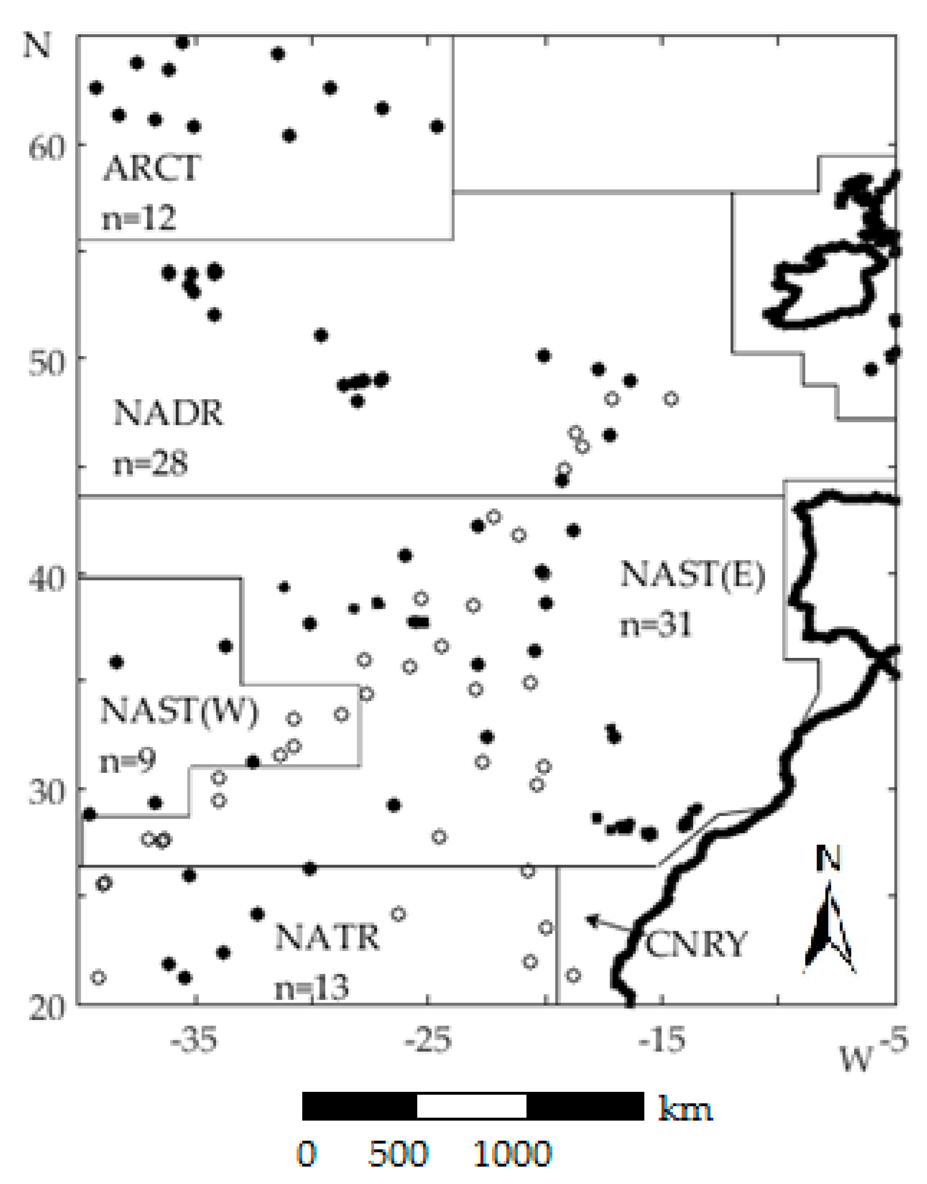
Figure 1. Stations sampled for the determination of in situ integrated daily water column primary production (PPeu) in the North East Atlantic. Filled circles are stations sampled in summer; open circles are stations sampled in autumn.
Remotesensing 10 01116 g001
Figure 2. Photosynthesis-irradiance functions of the models used in the study: Solid lines—without photoinhibition, dotted lines—with photoinhibition.
Remotesensing 10 01116 g002
Figure 3. Scatter plots of log satellite and in situ PPeu [mg C m−2 day−1] in the NEA using daily OC-CCI data (N = 46) for (a) PPVGPM, (b) PPPSM, and (c) PPAph. Solid line is the 1:1 line; dotted line is the linear regression.
Remotesensing 10 01116 g003
Figure 4. Scatter plots of log satellite and in situ PPeu [mg C m−2 day−1] in the NEA using eight day OC-CCI composites (N = 95); (a) PPVGPM with photoinhibition, (b) PPPSM with photoinhibition, (c) PPAph with photoinhibition, (d) PPVGPM with no photoinhibition, (e) PPPSM with no photoinhibition, and (f) PPAph with no photoinhibition. Filled circles are data collected during summer; open squares are autumn data. Solid line is the 1:1 line; dotted line is the linear regression.
Remotesensing 10 01116 g004
Figure 5. Taylor diagram of log satellite and in situ PPeu [mg C m−2 day−1] for the NEA using eight day OC-CCI composites (N = 95). SD—solid arc, centre-pattern RMSE—dotted arc, r—dashed lines with a dot.
Remotesensing 10 01116 g005
Figure 6. Spatial distribution of satellite PPeu [mg C m−2 day−1] using OC-CCI climatology for 1998–2011 for; (a) PPVGPM in summer (June–August), (b) PPPSM in summer, (c) PPAph in summer, (d) PPVGPM in autumn (September–November), (e) PPPSM in autumn, and (f) PPAph in autumn.
Remotesensing 10 01116 g006
Figure 7. Spatial transects of satellite PPVGPM, PPPSM, and PPAph [mg C m−2 day−1] along 20° W from 20 to 60° N for (a) summer (June–August) and (b) autumn (September–November) using OC-CCI climatology for 1998–2011.
Remotesensing 10 01116 g007
Figure 8. Box-whisker plots for the sensitivity analysis on (a) PPVGPM, (b) PPPSM, and (c) PPAph: For the left hand y-axis, PP is from 0–4400 mg C m−2 day−1; right y-axis PP is from 0–1200 mg C m−2 day−1. Chl90 is the average Chl a concentration over the first optical depth, kd is the downwelling diffuse attenuation coefficient, I0 is the daily surface PAR, PBopt is the biomass-specific optimum rate of photosynthesis, DL is the day length, PBm is the biomass-specific maximum rate of photosynthesis, αB is the initial slope of the P-I curve, aph (443) is the coefficient of light absorption by phytoplankton at 443 nm, φm is the maximum quantum yield of photosynthesis, and Kφ is the half-saturation constant of the φ-I curve. The rectangular boundaries are the first and third quartiles (the 25th and 75th percentiles) of the modelled PPeu obtained by changing each parameter in turn. The line in the rectangle is the median (50th percentile) of the sample, the edges of the “whiskers” are the size of the sample (minimum and maximum of the sample), and the symbol, “o”, represents extreme values. The larger the size of the box and whiskers, the greater the contribution of the parameter to the variability in the modelled PPeu.
Remotesensing 10 01116 g008
Figure 9. Box-and-whisker diagram from the sensitivity analysis for PPVGPM, PPPSM, and PPAph in the ARCT province. Chl a and aph (443) were changed in the models based on the variability in values at stations.
Remotesensing 10 01116 g009
Figure 10. Histograms of the coefficient of variation of satellite PPeu for the area of 12 × 12 km (3 × 3 pixels) for each match-up station analysed using eight day composite data (N = 95) for (a) PPVGPM; (b) PPPSM; and (c) PPAph and using daily data (N = 46) with (d) PPVGPM; (e) PPPSM; and (f) PPAph.
Remotesensing 10 01116 g010
Table 1. Provinces and time periods for in situ integrated daily water column primary production (PPeu) (mg C m−2 day−1) used for the accuracy assessment of the primary production satellite models.
RegionNorth East Atlantic (NEA): 20–65° N, 5–40° W
Period1998–2013
Number of stations (n)95
Seasons 1
summer, n = 56June-1998, July–August 2002, June-2003, May-2004, June-2005, July–August 2007, August-2009
autumn, n = 38September-2003, September-2004, October-2008, September-2009, October-2011, October-2012, October-2013
ProvincesARCT 2—Atlantic Arctic Province (n = 12)
NADR—North Atlantic Drift (n = 28)
NAST 3—North Atlantic Subtropical Gyre (East & West) (n = 40)
NATR 4—North Atlantic Tropical Gyre (n = 14)
1 When all stations were considered together, additional data from April 2002 were also included. 2 Biogeographical provinces were defined following [35]. 3 Analysis of stations in NAST(W) and NAST(E) were merged into NAST. 4 One station from CNRY (Canary Current Coastal province) was added to stations in NATR.
Table 2. Average and range of photosynthetic parameters used in PPPSM and PPAph: αB [mg C (mg Chl)−1 h−1 (μ E m−2 s−1)−1], PBm [mg C (mg Chl)−1 h−1], and φm [mole C E−1].
αBPBmφm
N122913
mean0.0493.3160.032
SD0.0192.1530.016
min0.0170.9470.010
max0.0789.1360.060
Table 3. Relative percentage difference (%) between modelled PPeu with and without photoinhibition. The negative sign “−” indicates how much photoinhibition reduces PPeu.
ModelMeanMinMax
PPVGPM−7−2−10
PPPSM−42−20−50
PPAph−11−4−15

