Single-Polarized SAR Classification Based on a Multi-Temporal Image Stack

Abstract

Land cover classification plays a pivotal role in Earth resource management. In the past, synthetic aperture radar (SAR) had been extensively studied for classification. However, limited work has been done on multi-temporal datasets owing to the lack of data availability and computational power. As Earth observation (EO) becomes more and more imperative, it becomes essential to exploit the information embedded in multi-temporal datasets. In this paper, we present a framework for SAR pixel labeling. Specifically, we exploit spatio-temporal information for pixel labeling. The proposed scheme includes four steps: (1) extraction of spatio-temporal observations; (2) feature computation; (3) feature reduction and (4) pixel labeling. First, an adaptive approach is applied to the data cube to extract spatio-temporal observations in both coherent and incoherent domains. Second, features in distinct domains are designed and computed to boost information content embedded in the multi-temporal datasets. Third, sequential feature selection is utilized for selecting the most discriminative features among the entire feature space. Last, the discriminative classifier is used to label the class of each pixel. By integrating pixel-/object-based processing techniques, spatial/temporal observations and coherent/incoherent data attributes, the proposed method explores diverse observations to solve complex labeling problems. In the experiments, we apply the proposed method on 64 TanDEM-X images and 70 COSMO-SkyMed high-resolution images, respectively. Both experiments reveal high accuracies for multi-class labeling. The proposed technique, therefore, provides a new solution for classifying multi-temporal single-polarized datasets.

1. Introduction

Classifying land cover type has become more and more pivotal as remote sensing technology advances. Among the existing techniques, optical images are one of the most commonly applied data for the classification purposes [1]. The high spatial and spectral resolution drastically helps verify land cover of the Earth’s surface. However, optical images are seriously restricted by atmospheric and radiometric conditions, which hamper the data availability for classification purposes. In contrast, synthetic aperture radar (SAR) systems sense the Earth’s surface through the active microwave. It is, therefore, less restrained by the atmospheric and radiometric effects, making it possible to have a solid temporal resolution that meets the demand of continuous observation. For these reasons, SAR sensors are able to play a major role in several application domains dealing with the production of land cover maps, especially in cases in which optical sensing fails due to the unavailability of cloud-free data [2].

However, the coherent nature of radar signals can cause the effect of speckle [3] and lead to low signal-to-noise ratios in the acquired images. The backscattering energy collected by the SAR systems may also fluctuate due to different reasons, such as differences in moisture content, alterations in incident angles and interventions of human activities. More importantly, the lack of spectral characteristics impedes the capability of discerning different ground features from SAR data. Thus, it is hard to obtain high classification accuracies if only one single-polarization SAR image is considered [2]. To efficiently mitigate these effects, one will have to explore the possibilities in two aspects: (1) utilizing more complex datasets or (2) increasing the information content of processing units.

The first aspect can be characterized into three types: (1) polarimetric datasets; (2) integrated datasets and (3) multi-temporal datasets. The first category, polarimetric datasets (i.e., PolSAR), has not only the advantages of conventional SAR systems, but also the capabilities of capturing more information about the backscattering characteristics. Therefore, it has been extensively investigated in past studies [4,5]. The second category focuses on the integrated datasets among multi-sensor/frequency/polarization data. In [6], SAR images were fused with multi-spectral images to acquire accurate land cover maps. However, multi-spectral images are often not available in operational applications [2]. In [7], multi-polarization images were used for land cover mapping. In [8,9,10], multi-frequency multi-polarization SAR images were applied. Despite favorable classification performances of these datasets, they are limited to airborne SAR systems so far. The last category, as presented in this study, focuses on the temporal signature of a single-polarized data stack. In [11,12], the temporal variability of the backscatter coefficient was utilized. The work in [11] conducted crop classification based on an interactive human/computer procedure. The most distinct image features were classified by photo-interpretation first. Then, image analysis was carried out on the less interpretable image features. The work in [12] addressed a two-class problem (forest/non-forest) based on a rule-based procedure. Areas with low temporal variability were considered as the non-forest regions. The work in [2] addressed the four-class (urban/field/forest/water) and two-class (forest/non-forest) problems using both coherent and incoherent data. It first qualitatively selected a few estimators as features specifically for the class in question and then considered the features as inputs of the RBF (radial basis functions) neural network classifier. The work in [13] utilized the time series of backscatter coefficients for crop classification. Although the past studies in this category revealed the potential of SAR classification, solutions for higher automation and the multi-class problem are still in the development stage.

The second aspect, which focuses on the information content of processing units, also plays a key role in the classification performance. Processing units are related to the basic size on which the image operation performs. They can be divided into three groups: (1) single pixels; (2) clustered pixels and (3) combinations of pixels, clusters and other information. The first type is referred to as the pixel-based image analysis (PBIA). It has been extensively applied to SAR data because of its simplicity and efficiency [4,5]. As PBIA takes single pixels as basic units without considering the correlation of nearby pixels, it usually requires spatial filtering to reduce the speckle effect. In this sense, the full resolution is not available in most cases. The second type is referred to as the object-based image analysis (OBIA). Different from PBIA, OBIA extracts image objects based on an image segmentation process and then performs the image analysis on the objects. Since the objects represent groups of pixels that share similar characteristics, OBIA can improve the information content of the processing units and provide improvements over PBIA. However, OBIA commonly requires a systematic trial/error approach with visual inspection of the image objects for the set up of suitable segmentation [14]. Over-/under-segmentation problems may take place for complex scenes that contain different land cover classes. An error amplification phenomenon can thus occur [14]. The last type, as proposed in this study, is hybrid image analysis. Hybrid image analysis refers to the use of multiple processing units within the analysis framework. The work in [15] performed maximum likelihood classification at the pixel level followed by the nearest-neighbor classification at the object level. The integrated method outperformed the results that utilized PBIA/OBIA alone. Overall, limited studies have been carried out on hybrid image analysis for SAR classification.

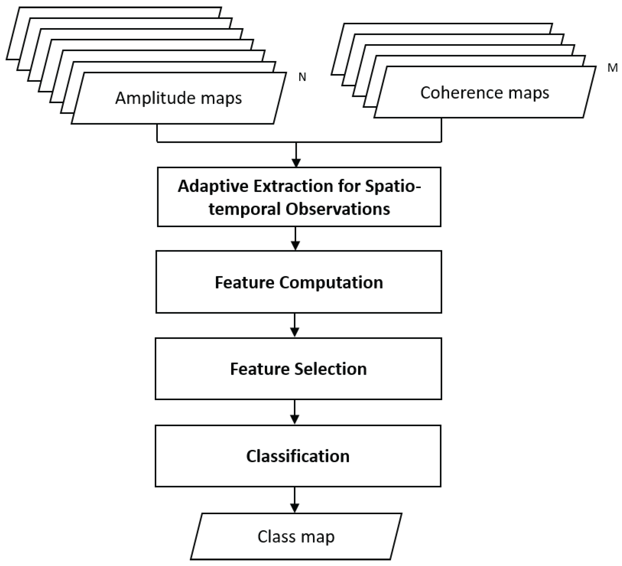
Pixel labeling for SAR images has been studied in various ways. Nevertheless, limited studies have been done on multi-temporal datasets. As the need for continuous observation arises drastically, multi-temporal datasets become much more available than before and thus build up new routes for image analysis. In this paper, we present a framework built upon a high-level of utilization of multi-temporal datasets for classifying single-polarized images. Our method integrates spatial/temporal and coherent/incoherent observations with pixel-based/object-based analysis to improve the classification accuracy. In the following, we focus on same-sensor same-incidence SAR datasets and consider land cover mapping as our primary goal. The proposed framework is shown in Figure 1. The framework shows the procedures of the proposed method, including (1) the multi-temporal data stack; (2) adaptive extraction of spatio-temporal observations and (3) algorithms that consider spatio-temporal observations conjointly for certain applications.

The main novelties of the proposed method consist of the following: first, spatio-temporal observations are extracted and utilized based on local homogeneity. The pixel-based information is used for isolated targets, and the object-based information is used for homogeneous targets. Second, innovative features in spatial/temporal and coherent/incoherent domains are designed to enrich the information content limited to single-temporal single-polarized datasets. Lastly, a favorable generalization can be achieved. Different methods and applications can be incorporated into the proposed framework.

This paper is organized into four sections. Section 2 details the methodology, including the extraction of spatio-temporal observations, feature computation, feature selection and pixel labeling. Section 3 describes study areas and datasets. Our experiments use TanDEM-X and COSMO-SkyMed datasets to validate the proposed approach. Section 4 presents the experimental results and discussions. Section 5 draws the conclusions.

2. Methodology

2.1. Adaptive Extraction of Spatio-Temporal Observations

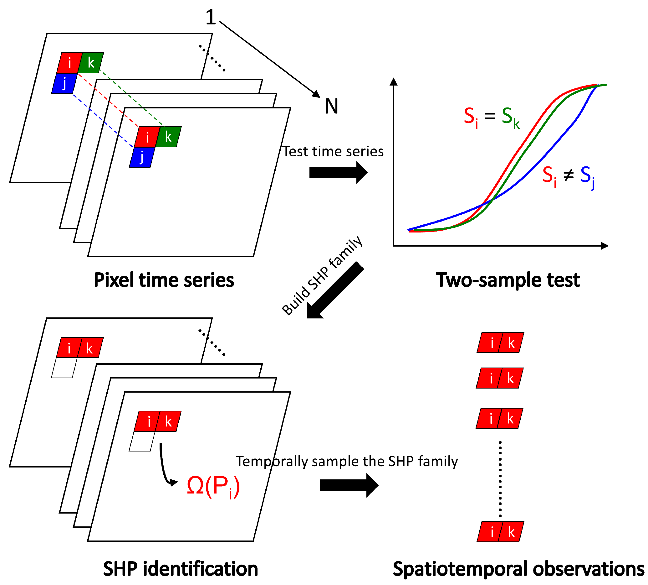
Multi-temporal datasets contain long series of observations of the same imaged regions. Since their amplitude time series can provide useful information of the characteristics of the imaged areas, many studies utilized these time series to find homogeneous regions for adaptive image processing (e.g., spatial filtering [16,17] and complex coherence estimation [18]). The members of the homogeneous region with respect to a pixel-of-interest are commonly referred to as statistically-homogeneous pixels (SHP) [16]. As SHP share similar backscattering properties in the time domain, processing images based on SHP reduces the impact of irrelevant information. To improve the information content of the processing units, we develop a strategy to extract spatio-temporal observations that are adaptive to the local homogeneity. As illustrated in Figure 2, the procedures include two steps: (1) SHP identification and (2) temporal sampling.

A common approach for SHP identification is through hypothesis testing. To allow a self-contained reading of this study, we briefly describe the required steps of SHP identification. A detailed description can be found in [16]. Assume N SAR images were acquired in the same geometry, having been well coregistered and geometrically corrected. One can acquire an amplitude time series by temporally sampling a generic pixel P:

$$\mathit{I}\left(P\right)={[I_1\left(P\right),I_2\left(P\right),\dots ,I_N\left(P\right)]}^T$$

(1)

where $\mathit{I}\left(P\right)$ represents the amplitude time series from the first to the N-th images and ${}^T$ is the transposition.

We then perform the hypothesis tests on $\mathit{I}\left(P\right)$ and $\mathit{I}\left(P_{kn}\right)$ by defining a K-neighborhood estimation window centering on P:

$$\left\{\begin{array}{cc}{H}_0:\hfill & S_{\mathit{I}\left(P\right)}=S_{\mathit{I}\left(P_{kn}\right)}\hfill \\ H_1:\hfill & S_{\mathit{I}\left(P\right)}\ne S_{\mathit{I}\left(P_{kn}\right)}\hfill \end{array}\right.$$

(2)

where $kn\in [1,K]$ and S indicates a similarity measure.

Various similarity measures (e.g., Kolmogorov–Smirnov and Anderson–Darling tests) have been applied for SHP identification. However, these tests cannot handle possible temporal variability. To reduce the impact of temporal variability during the SHP identification process, we apply the robust t-test (TR) developed in our recent studies (see [19] for details) to improve the effectiveness of the test operation. The application of the TR test helps to identify the SHP with assurances of similar temporal behaviors.

If the null hypothesis (i.e., $H_0$) is not rejected at a given significance level, P and $P_{kn}$ will be considered statistically homogeneous. $P_{kn}$ will be incorporated into the SHP family $\Omega \left(P\right)$. Once $\Omega \left(P\right)$ is identified, we can acquire the spatio-temporal observations for either incoherent (the incoherent data stack represents the amplitude maps, which are related to the backscatter coefficients) or coherent (the coherent data stack indicates the coherence maps, which are related to the interferometric observations) data stacks. One can acquire the incoherent spatio-temporal observations by temporally sampling the amplitude data stack:

$$\mathit{I}(\Omega \left(P\right))=[\mathit{I}\left(P_1\right),\mathit{I}\left(P_2\right),\dots ,\mathit{I}\left(P_q\right)]$$

(3)

or acquire the coherent spatio-temporal observations by temporally sampling the coherence data stack:

$$\mathit{C}(\Omega \left(P\right))=[\mathit{C}\left(P_1\right),\mathit{C}\left(P_2\right),\dots ,\mathit{C}\left(P_q\right)]$$

(4)

where q indicates the size of $\Omega \left(P\right)$. $\mathit{C}\left(P\right)$ represents a column vector of coherence values.

Applying the extracting operation to each pixel, we obtain a spatio-temporal cube that contains a group of observations sharing similar statistical characteristics in both incoherent and coherent domains.

2.2. Feature Computation for Information Extraction

To differentiate distinct land cover types, we need certain indexes to depict the information embedded in images. These indexes are usually referred to as “features”. As $\mathit{I}(\Omega (P\left)\right)$ and $\mathit{C}(\Omega (P\left)\right)$ provide abundant information in both time and space, various features can be developed. In this study, we design four categories of features. A total of 52 features has been developed. To focus on the scope of this study, we qualitatively describe these entities as follows:

• Time series features: These features are related to the group statistics of $\mathit{I}(\Omega (P\left)\right)$ and $\mathit{C}(\Omega (P\left)\right)$. We design these features by adjusting the processing order of logarithm (log), mean, standard deviation (std), saturation, etc. With different combinations, various statistics can be calculated. For example, one can first compute the spatial average of $\mathit{I}(\Omega (P\left)\right)$ to obtain a time series vector and then calculate the standard deviation of this vector, and vice versa. One can also compute a single mean or a single std of $\mathit{I}(\Omega (P\left)\right)$ or $\mathit{C}(\Omega (P\left)\right)$.
• SHP features: These features represent the statistics specifically regarding the SHP. For example, one can first compute the SHP size at each pixel (i.e., area of $\Omega \left(P\right)$), obtaining an SHP size map. Then, the mean or std of $\Omega \left(P\right)$ can be calculated based on the SHP size map to acquire different SHP features.
• Textural features: These features analyze the statistics of spatial relations among neighboring pixels (e.g., smoothness, roughness, periodicity). Different types of textural features have been developed (see [20]). As we have obtained the spatial contents through $\Omega \left(P\right)$, we can compute each of these features accordingly. We implement several textural features (e.g., energy and entropy) based on the gray level co-occurrence matrix (GLCM) (GLCM utilizes the second-order statistics of the grayscale image histograms to calculate the textures) [21]. We acquire these features using the reflectivity map (temporal average of the incoherent data stack) and the long-term coherence map (temporal average of the coherent data stack).
• Geometric features: These features measure the geometric characteristics of $\Omega \left(P\right)$. Many intuitive features can be computed, such as the border length, shape index, compactness, asymmetry, etc. These features have been extensively used in OBIA as they provide spatial information that is not well depicted in PBIA.

Assume M features have been computed ($M=52$ in this study). In this sense, we transform the single-polarized data stack into an M-layer feature stack. The computed features for P can be represented as:

$$\mathit{f}\left(P\right)={[f_1\left(P\right),f_2\left(P\right),\dots ,f_M\left(P\right)]}^T$$

(5)

where $\mathit{f}\left(P\right)$ represents an M-element feature vector.

2.3. Feature Selection for Dimensionality Reduction

The feature computation step provides an adequate number of feature responses at each pixel. In such a case, it is impractical to manually manage these features for classification. Supervised classification is also confronted with challenges related to the unbalance between limited training sets and high-dimensional feature responses. This effect results in unreliable estimation of statistical class parameters [22]. As a consequence, the classification accuracy tends to decrease as the number of features increases [23] (known as the Hughes effect [24]). Data mining or machine learning techniques thus become pivotal in terms of information extraction as they can discover representative/discriminative features from the obtained feature stack.

Dimensionality reduction is a useful approach for this scope. It can be categorized into two types: (1) feature selection and (2) feature extraction [25]. The former aims at selecting a subset of features that minimizes redundancy and maximizes relevance to the class labels, whereas the latter transforms the original features into a new feature space using combinations of the original ones. Feature selection chooses representative features from the original feature space without transformation. It, therefore, preserves the physical meanings of the selected features. In this sense, feature selection is superior in terms of better readability and interpretability [26].

To improve the accuracy of classification and boost the performance on a high-dimensional feature stack, we apply one of the best known feature selection approaches, sequential forward selection (SFS) [27], for dimensionality reduction. The SFS is based on a local search for solutions defined by the current solution state. Compared with other types of searching strategies (e.g., exponential searching), SFS has a considerably low computational cost. The implementation of SFS is simple in concept. First, the algorithm starts with an empty feature set. Then, it iteratively brings in a feature $f_i$ (where $i\in [1,M]$) by evaluating Equation (6) until the inclusion of $f_i$ no longer improves a predefined criterion function G.

$$f_m^s=f_{m-1}^s\cup \underset{f_i}{argmax}\left\{G(f_{m-1}^s\cup f_i,T,R)\right\}$$

(6)

where $f^s$, T and R represent the selected feature set, training set, as well as classification model/parameters, respectively. m denotes the size of the up-to-date selected feature set.

The SFS is generally used as wrapper feature selection algorithms such that the criterion function G is assessed through a classifier R trained and evaluated on different parts of the training set T [28]. Different criterion functions and classifiers can be applied. We select the classification accuracy and discriminant analysis (DA) [29] (see Section 2.4) as the criterion function and the classifier. Because SFS applies the greedy search algorithm based on a hill-climbing scheme for optimizing the criterion function G, it is susceptible to the local extremum with respect to the feature set S. We thus incorporate the leave-one-out cross-validation (LOO-XV) [30] with the SFS to avoid local optimal solutions. By applying these procedures, we reduce the feature size from M to m, where m is considerably less than M. The selected feature set becomes:

$${\mathit{f}}^{\mathbf{s}}\left(P\right)={[f_1^s\left(P\right),f_2^s\left(P\right),\dots ,f_m^s\left(P\right)]}^T$$

(7)

The selected feature set ${\mathit{f}}^s$ represents the most discriminative features among the original features $\mathit{f}$. Therefore, we take ${\mathit{f}}^s$ as the input of pixel labeling.

2.4. Pixel Labeling

Various classifiers can be used for pixel labeling. They can be categorized into parametric and nonparametric ones depending on the probability density estimation approach. Parametric classifiers assume the form of density functions for each class and estimate the corresponding parameters through training sets. Nonparametric classifiers compute the local densities through training sets without specifying the form of density function. However, parametric methods usually require less computation and storage than the nonparametric ones. They also perform fairly well for practical problems. In this sense, we select a benchmark classifier (DA) to validate the effectiveness of the proposed framework. Depending on how the covariance matrices are assumed, DA can have different forms, such as LDA (LDA assumes that the Gaussians for each class share the same covariance matrix) (linear decision surface) and QDA (QDA has no assumptions on the covariance matrices of the Gaussians) (quadratic decision surface). The DA classifier has several advantages. Its solution is in closed form, which can be efficiently computed. Furthermore, it is inherent in multi-class problems. Moreover, it does not require tuning the hyperparameters. In this study, we employ the QDA classifier for both feature selection and classification to show the potential of the proposed framework. Compared with LDA, QDA is able to learn quadratic boundaries between different classes and is thus more flexible.

3. Study Areas and Data Description

To evaluate the effectiveness of the proposed framework, we carry out two experiments using high resolution datasets. These experiments aim at solving the multi-class problem using the single-polarized data stack.

3.1. TanDEM-X Data Stack in Los Angeles

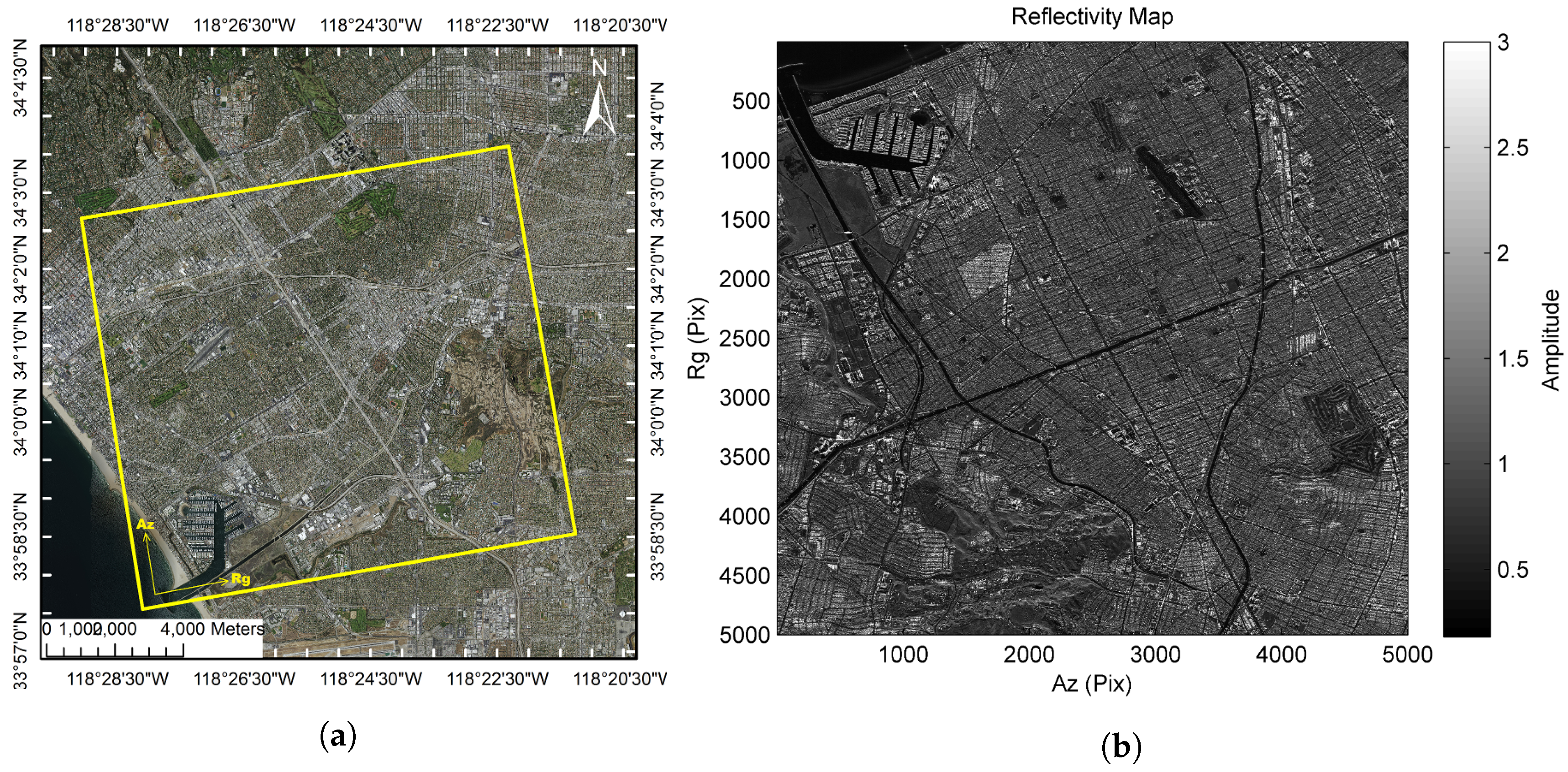
The study area of this dataset is located in Los Angeles, California, the United States. As shown in Figure 3, this area contains various ground features, including roads, water, bare soils, grasses, trees and urban areas. This dataset consists of 64 images collected between October 2010 and January 2014. The images were acquired in ascending orbit with HH (horizontal-transmit-horizontal-receive) polarization. The incidence angle was 41.02${}^{\circ }$, and the spatial resolution in range and azimuth was 2.08 m and 1.89 m, respectively. The dimensions of these images are 5000 × 5000 pixels. To assess the classification performance, we manually select training and testing sets based on visual interpretations of optical imagery (the optical image was taken from Landsat on 11 August 2013) from Google Earth [31]. The selections and the corresponding sizes are shown in

Table 1. Number of training and testing pixels for the TanDEM-X dataset.

Class	Training Set	Testing Set
Road	3959	215,243
Water	13,580	336,003
Bare Soil	8177	327,836
Grass	1654	18,650
Tree	2130	24,761
Urban	9821	171658
Total	39,321	1,094,151

and Figure 4, respectively.

3.2. COSMO-SkyMed Data Stack in Chicago

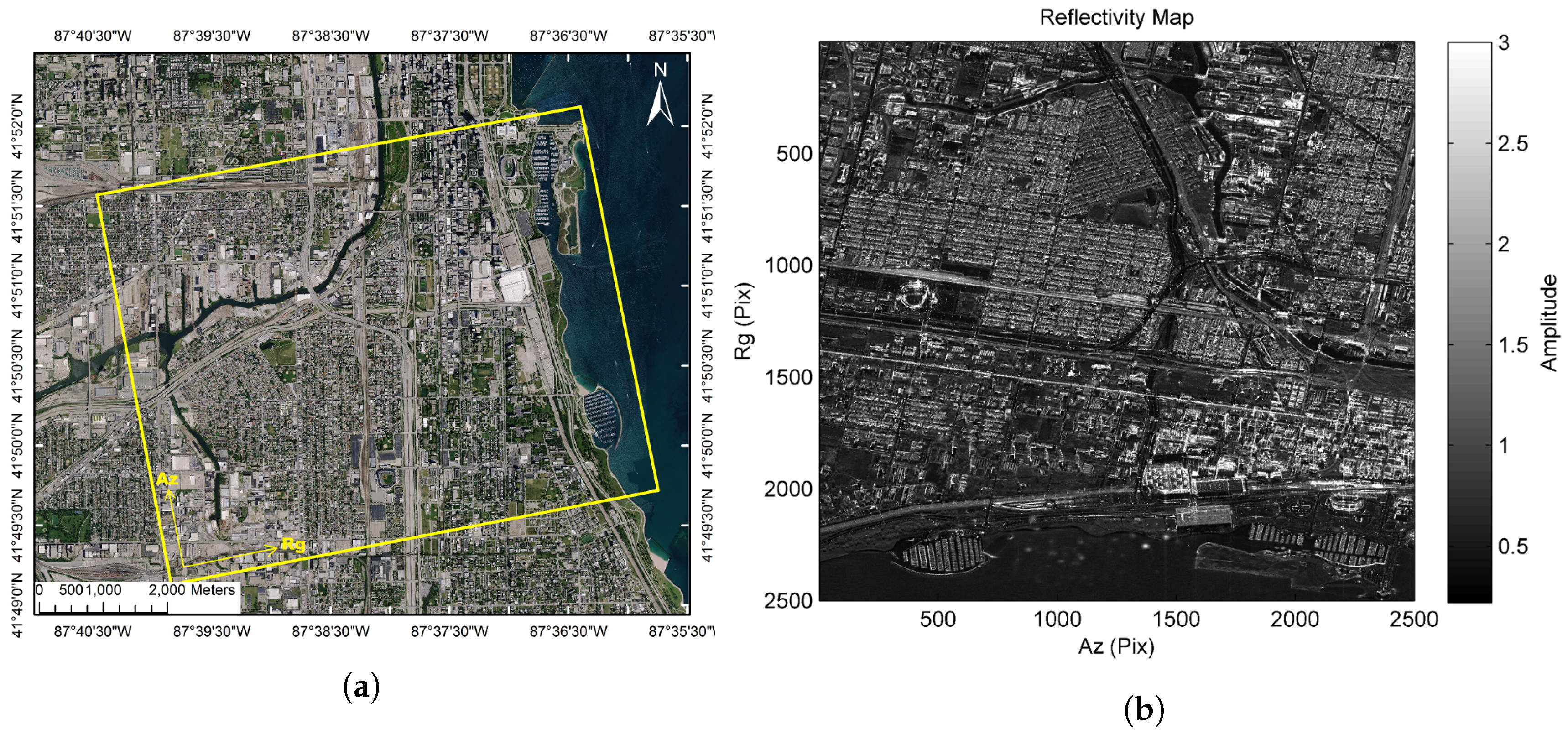
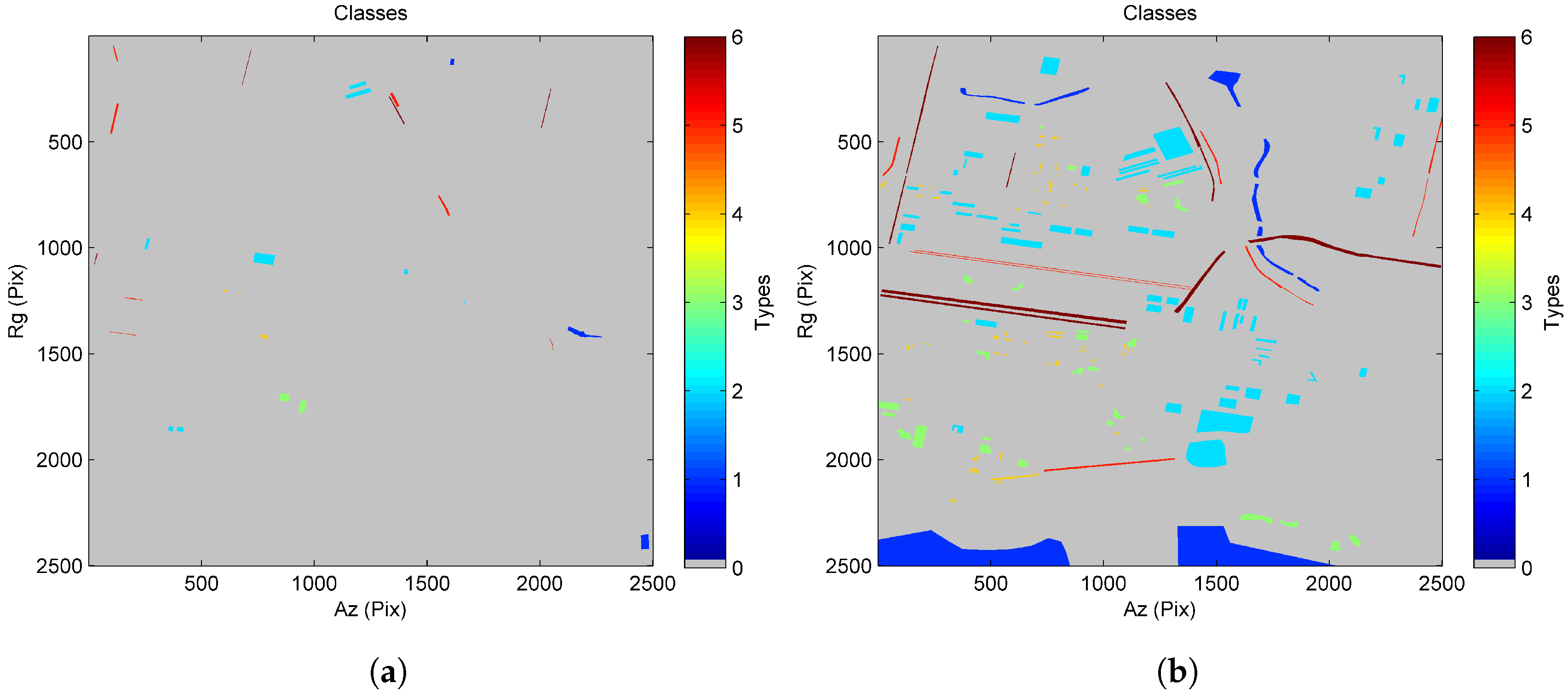
The study area of this dataset is located in Chicago, Illinois, the United States. As shown in Figure 5, this area contains several land cover types, including water, urban areas, grasses, trees, railroads and roads. This dataset consists of 70 images collected between January 2013 and December 2014. The images were acquired in ascending orbit with HH polarization. The incidence angle was 23.93${}^{\circ }$, and the spatial resolution in range and azimuth was 2.40 m and 1.80 m, respectively. The dimensions of these images are 2500 × 2500 pixels. To assess the classification performance, we manually select training and testing sets based on visual interpretations of optical imagery (the optical image was taken from Landsat on 2 April 2013) from Google Earth [32]. The selections and corresponding sizes of training and testing sets are shown in

Table 2. Number of training and testing pixels for the COSMO-SkyMed dataset.

Class	Training Set	Testing Set
Water	5168	189,506
Urban	9970	163,348
Grass	3009	39,018
Tree	619	11,270
Railroad	4228	19,788
Road	2029	55,139
Total	25,023	478,069

and Figure 6, respectively.

4. Experiments and Discussions

Using the proposed approach, the proposed system first acquires a full feature vector $\mathit{f}$ for each pixel (the length of $\mathit{f}$ is 52 in this study). Then, our system employs the SFS to find f${}^s$, which represents the most discriminative features among all the computed features. Last, it applies the QDA classifier to f${}^s$ to label the class of each pixel.

In both experiments, we compare the results with Skriver’s approach [13], which utilizes the time series of backscatter coefficients to classify the single-polarized dataset. We also use the feature set suggested in [2] to see the impact of a different feature choice. Furthermore, we employ random picks of training and testing pixels to understand the stability of the selected feature sets. We combine the training and testing sets into a single set and then perform repeatedly the classification using random picks of 10% of the pixels in this set as training data (leaving the remaining 90% for validation). By repeatedly performing this procedure 100 times, we compute the average and standard deviation of the classification performances. Other commonly-used classifiers (e.g., LDA, decision tree, naive Bayes) are compared, as well, to verify the generalization of the proposed framework.

In all comparisons, we evaluate the classification performance based on the confusion matrix and its derivatives, such as the overall accuracy, producer’s accuracy, user’s accuracy and Cohen’s Kappa coefficient. The producer’s and user’s accuracies are related to omission and commission errors, respectively. The overall accuracy represents the correct rate of the overall classification. The Kappa coefficient indicates the global accuracy. The Kappa coefficient can assess the classification performance with favorable objectivity as it takes into account the possibility of the correctness occurring by chance.

4.1. Results for the TanDEM-X Data Stack

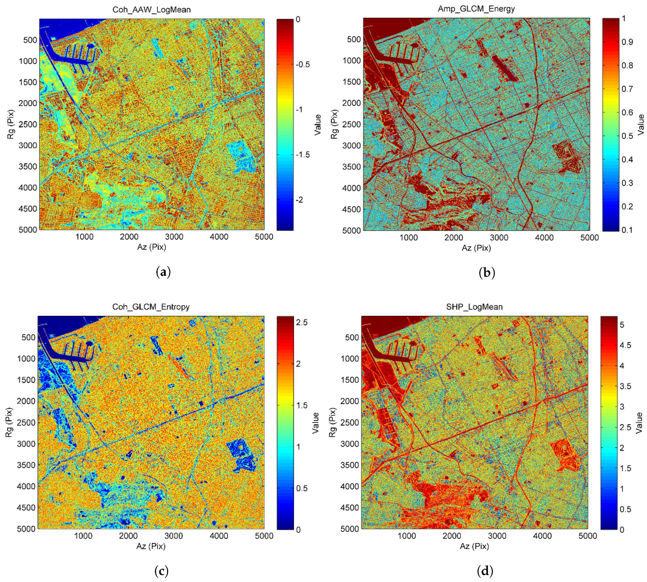
The selected features for the TanDEM-X data stack are shown in Figure 7. Figure 7a–d corresponds to the first to the fourth features selected by the SFS. This feature set leads to the highest classification accuracy during the SFS process. One can observe distinct responses of different land cover classes among these features. The first feature represents the log mean of $\mathit{C}(\Omega (P\left)\right)$. It shows the capability to distinguish between water, roads, bare soils and urban areas. The second feature is the GLCM (energy) of $\mathit{I}(\Omega (P\left)\right)$. This feature reveals the capability to differentiate between grasses and trees. It also shows the potential of separating roads from urban areas. The third feature is the GLCM (entropy) of $\mathit{C}(\Omega (P\left)\right)$. It can be used to separate vegetation from urban areas. The fourth feature is the log mean of $\Omega \left(P\right)$. This feature is useful for distinguishing between homogeneous (e.g., roads, water and bare soils) and isolated targets (e.g., urban areas).

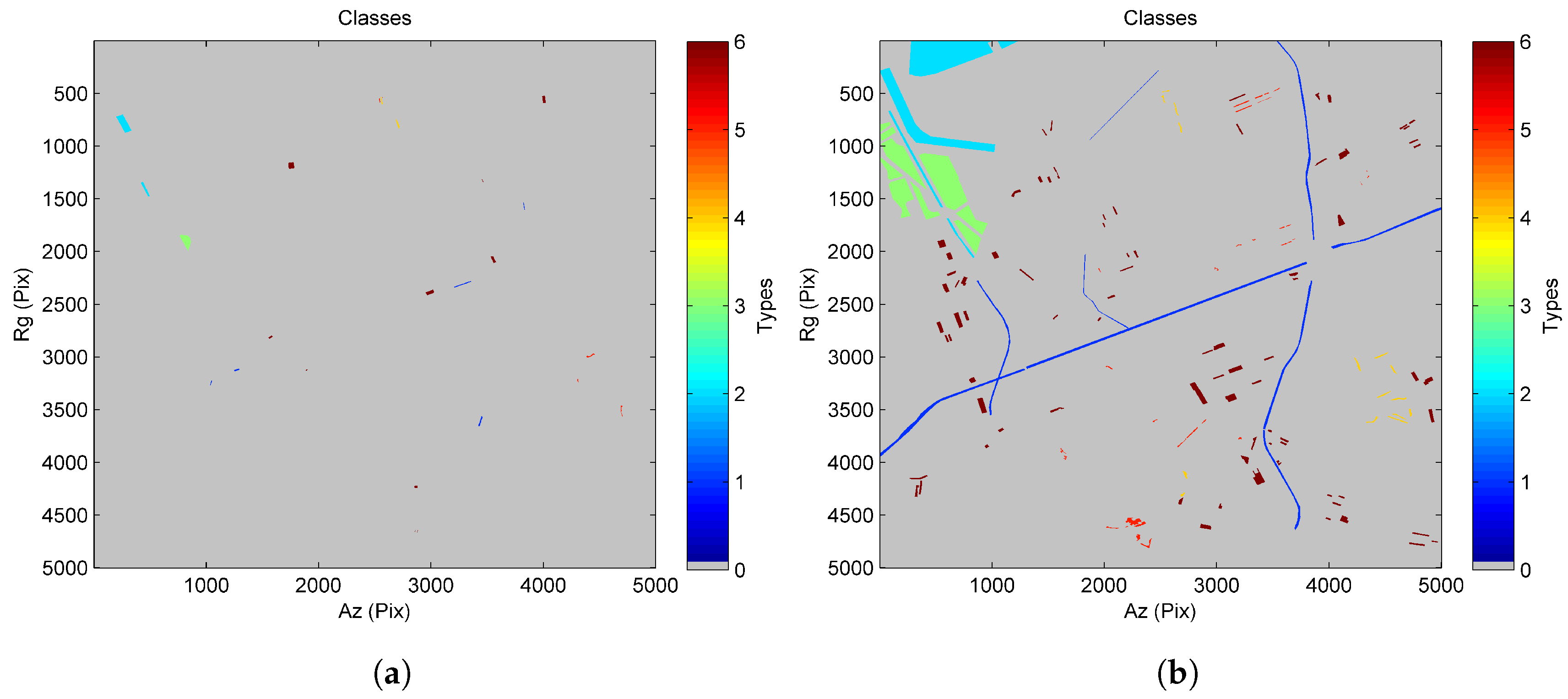
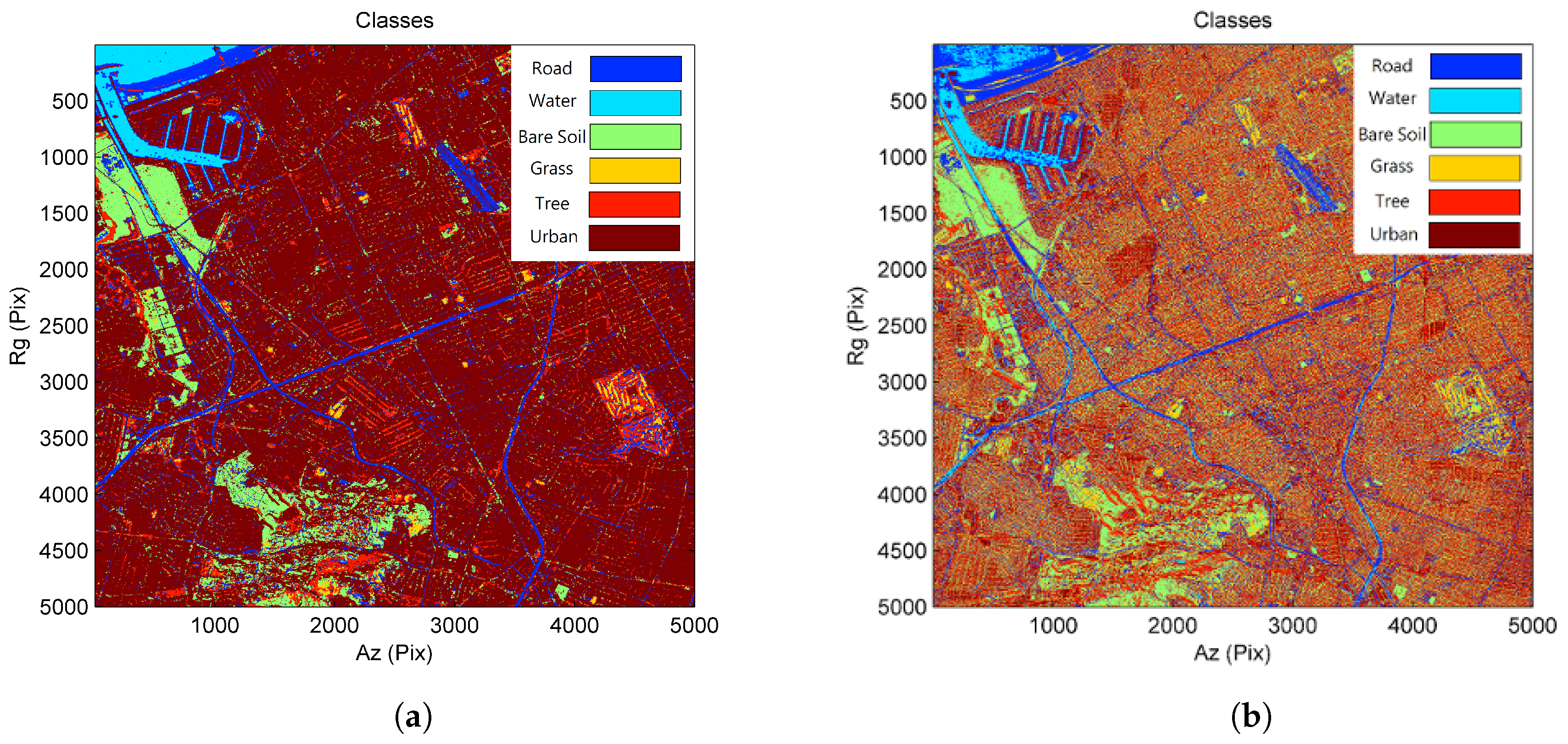
For the sake of simplicity, we illustrate the class maps of the proposed and Skriver methods in Figure 8. The confusion matrices for these two approaches are described in

Table 3. Confusion matrix for the TanDEM-X dataset based on the proposed approach.

		Classified						Producer’s Accuracy
		Road	Water	Bare Soil	Grass	Tree	Urban
Reference	Road	155,157	45	5086	1353	8572	45,030	72.08%
	Water	27,584	306,994	117	489	187	632	91.37%
	Bare Soil	16,126	0	287,988	6237	4998	12,487	87.85%
	Grass	7307	27	1368	6405	2885	658	34.34%
	Tree	644	0	563	0	12,241	11,313	49.44%
	Urban	6638	1	9311	373	1757	153,578	89.47%
	User’s accuracy	72.69%	99.98%	94.60%	43.11%	39.95%	68.65%	Overall accuracy: 84.30% Kappa coefficient: 79.32%

and

Table 4. Confusion matrix for the TanDEM-X dataset based on Skriver’s approach.

		Classified						Producer’s Accuracy
		Road	Water	Bare Soil	Grass	Tree	Urban
Reference	Road	139,688	23,325	13,571	7376	21,561	9722	64.90%
	Water	132,640	198,371	107	60	878	3947	59.04%
	Bare Soil	16,843	17	271,925	6243	31,775	1033	82.95%
	Grass	7019	147	2217	8408	810	49	45.08%
	Tree	780	30	5857	969	14,884	2244	60.11%
	Urban	20,939	512	32,095	10,266	61,536	46,310	35.85%
	User’s accuracy	43.94%	89.19%	83.47%	25.23%	11.32%	73.15%	Overall accuracy: 62.11% Kappa coefficient: 51.36%

, respectively. The results show that the proposed approach outperforms Skriver’s approach. The proposed method reaches 84.30% overall accuracy and a 79.32% Kappa coefficient, indicating a favorable classification result. Compared with Skriver’s approach, the proposed method has a significant improvement in both overall accuracy (22% higher) and the Kappa coefficient (28% higher). As the coherent data provide useful information for further characterizing the land cover types, the lower classification accuracies in Skriver’s approach may be due to the fact that no coherent information is considered in their approach.

By looking into the confusion matrices, one can observe that the proposed method has high potential to classify various land cover types. The classification accuracies for roads, water, bare soils and urban areas are high in terms of user’s and producer’s accuracies. These results signify that the selected feature set provides good separations for the considered land cover types. The user’s and producer’s accuracies for grasses and trees are slightly lower than other land cover types as these two classes share similar statistics (medium coherence, fluctuated backscatter coefficient and similar SHP size) that can be easily confused with other ground features.

Apart from Skriver’s approach, it is interesting to compare the results using different features, classifiers and training/testing sets.

Table 5. Comparison of classification performances for the TanDEM-X dataset. The subscript r relates to the random picks from 100 trials. The subscripts m and 2 indicate the feature sets selected by sequential forward selection (SFS) and [2], respectively.

	Overall Accuracy (%)	Kappa (%)
QDA${}^r$	89.25 ± 0.15	85.82 ± 0.20
QDA${}^m$	84.30	79.32
QDA${}^2$	77.14	70.02
Skriver’s Approach	62.11	51.36
LDA${}^m$	82.70	77.17
Naive QDA${}^m$	84.02	78.94
Naive LDA${}^m$	82.65	76.93
Decision Tree${}^m$	82.31	76.98

lists the comparison of classification performances. One can observe that the random picks of training and testing pixels (i.e, QDA${}^r$) can offer low variations and high averages on their classification performance, showing good stability of the proposed approach. Results not shown here also signify that the selected features are stable. At this site, only 11 features (out of 52) have ever been selected among the 100 trials, and four of them (corresponding to Figure 7) have been selected more than 95 times.

The proposed method (i.e, QDA${}^m$) provides the highest classification performance among all the comparisons. The feature set selected by the SFS performs better than the one used in [2], as well. It also works well on different classifiers since the overall accuracies and Kappa coefficients remain high. These results reveal the favorable generalization of the proposed framework.

4.2. Results for the COSMO-SkyMed Data Stack

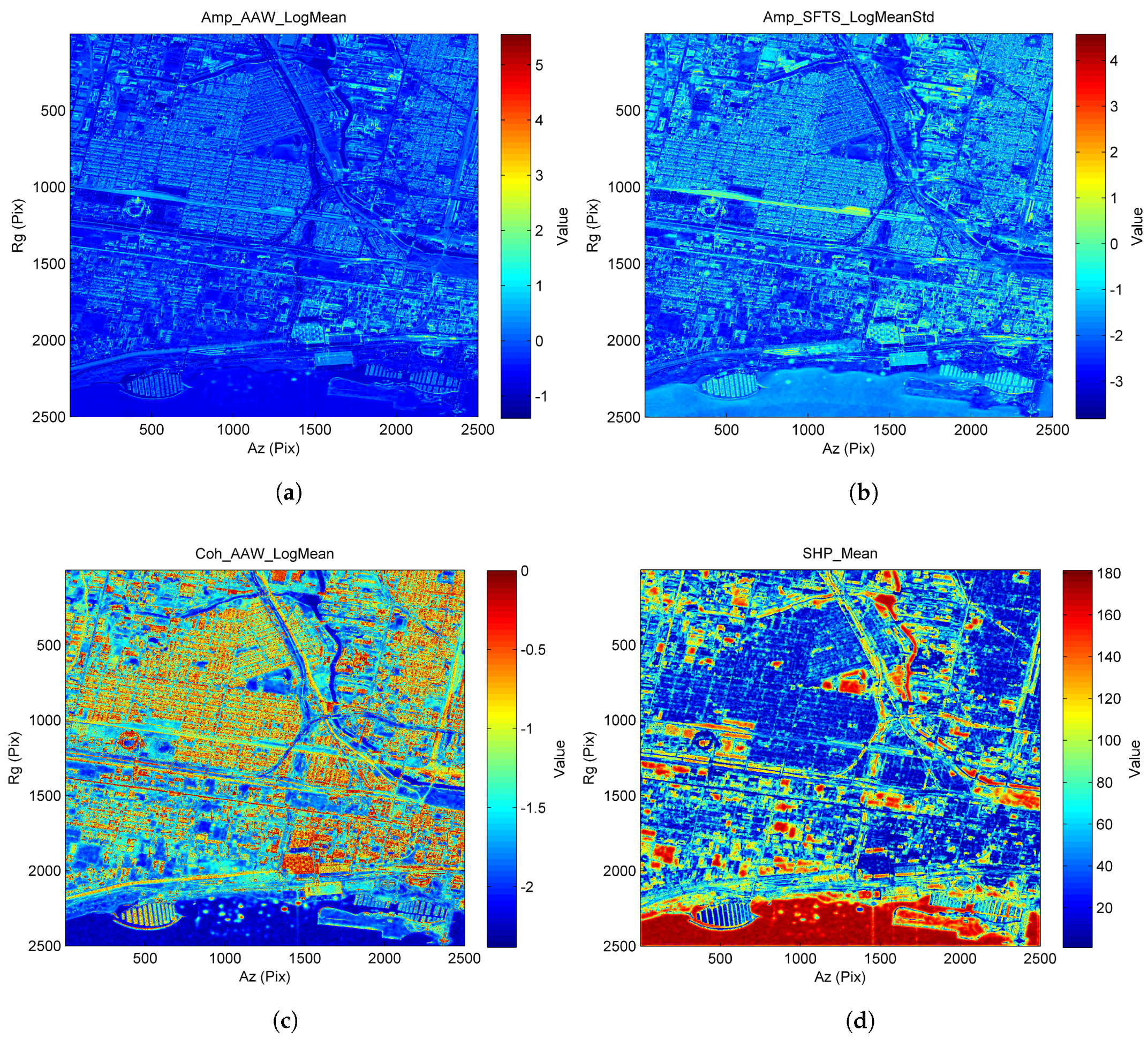
The selected features of the COSMO-SkyMed data stack are shown in Figure 9. Figure 9a–d corresponds to the first to the fourth features selected by the SFS. The first feature represents the log mean of $\mathit{I}(\Omega (P\left)\right)$. It has the capability to distinguish between urban areas and other types of land cover. The second feature is a statistic generated by taking the average in the spatial domain for $\mathit{I}(\Omega (P\left)\right)$, followed by computing the std in the temporal domain. This feature has the potential to separate between roads, railroads and urban areas. The third feature is the log mean of $\mathit{C}(\Omega (P\left)\right)$. It presents a favorable separation between roads and railroads. It can also be used to distinguish between water and urban areas. The fourth feature is the mean of $\Omega \left(P\right)$. It is useful for differentiating between trees and grasses. Water and urban areas are well separated by this feature, as well.

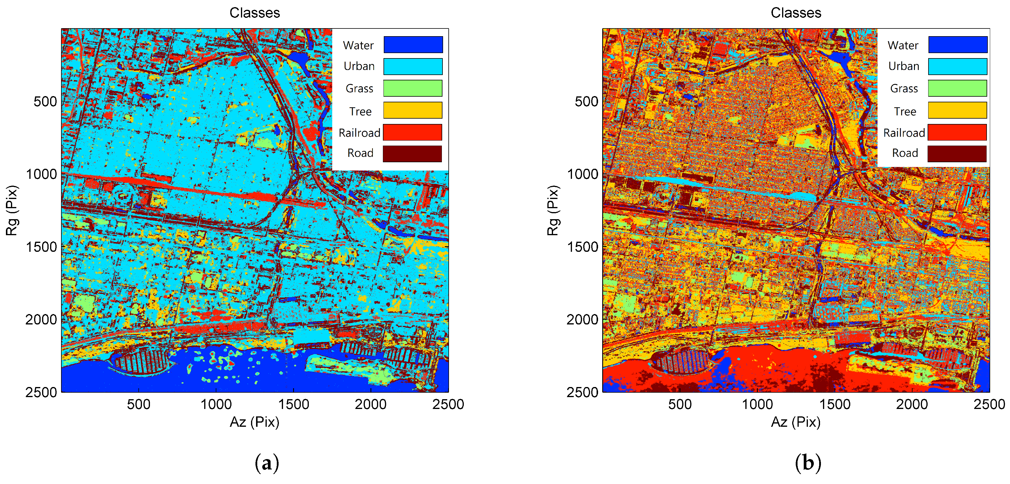
Similarly, we compare the results with Skriver’s approach, as shown in Figure 10. The corresponding confusion matrices are tabulated in

Table 6. Confusion matrix for COSMO-SkyMed dataset based on the proposed approach.

		Classified						Producer’s Accuracy
		Water	Urban	Grass	Tree	Railroad	Road
Reference	Water	176,643	1312	600	812	853	9286	93.21%
	Urban	1628	145,611	0	396	5461	10,252	89.14%
	Grass	304	4469	28,522	1661	389	3673	73.10%
	Tree	0	4610	0	5871	90	699	52.09%
	Railroad	0	5291	0	70	14,390	37	72.72%
	Road	1617	9530	0	110	2374	41,508	75.28%
	User’s Accuracy	98.03%	85.24%	97.94%	65.82%	61.09%	63.41%	Overall Accuracy: 86.29% Kappa Coefficient: 80.57%

and

Table 7. Confusion matrix for the COSMO-SkyMed dataset based on Skriver’s approach.

		Classified						Producer’s Accuracy
		Water	Urban	Grass	Tree	Railroad	Road
Reference	Water	35,336	709	226	813	79,473	72949	18.65%
	Urban	2882	41,610	3580	24,959	73,276	17,041	25.47%
	Grass	2	87	22,542	10,032	1323	5032	57.77%
	Tree	0	378	373	6781	3122	616	60.17%
	Railroad	0	6498	10	1590	11,625	65	58.75%
	Road	4914	3109	820	2787	9280	34,229	62.08%
	User’s Accuracy	81.92%	79.42%	81.82%	14.44%	6.53%	26.34%	Overall Accuracy: 31.82% Kappa Coefficient: 21.90%

, respectively. These results show that the proposed approach performs slightly better than the previous dataset. It achieves 86.29% overall accuracy and an 80.57% Kappa coefficient, which are considerably good as far as the multi-class problem is concerned. Skriver’s approach at this test site is less effective than the previous dataset. Its overall accuracy decreases from 62.11 to 31.82%, and its Kappa coefficient drops from 51.36 to 21.90%. One can observe remarkable increases in classification accuracies (overall accuracy is 54% higher and the Kappa coefficient is 59% higher) for the proposed method, signifying that our method is comparatively more stable than Skriver’s approach. Based on the confusion matrices, one can observe that different ground features are well classified under the proposed framework.

Specifically, when Skriver’s method and the proposed approach are compared, one can observe the remarkable differences in terms of the producer’s accuracy. The selected features capture the low reflectivity, low coherence and high homogeneity of the water areas, whereas Skriver’s method only considers the distribution of reflectivity. The limited information in Skriver’s approach can easily lead to the ambiguity between road and water, as they are both lowly reflected. A similar situation happens to urban areas, as well. The selected features signify the medium reflectivity, high coherence and low homogeneity of the urban areas, whereas Skriver’s method only utilizes the information of reflectivity, causing the ambiguity between man-made and vegetated areas, as well as the low accuracy of the classification.

Moreover, from the comparisons of different methods described in

Table 8. Comparison of classification performances for the COSMO-SkyMed dataset. The subscript r relates to the random picks from 100 trials. The subscripts m and 2 indicate the feature sets selected by SFS and [2], respectively.

	Overall Accuracy (%)	Kappa (%)
QDA${}^r$	89.64 ± 0.05	85.35 ± 0.07
QDA${}^m$	86.29	80.57
QDA${}^2$	77.41	67.11
Skriver’s Approach	31.82	21.90
LDA${}^m$	85.76	80.12
Naive QDA${}^m$	84.96	78.80
Naive LDA${}^m$	84.59	78.18
Decision Tree${}^m$	79.19	71.10

, we can also confirm that the proposed approach yields favorable performance and fairly appreciative generalization. Last but not least, the random picks of training and testing pixels can still provide low variations and high averages on their classification performance. These results reveal good stability of the proposed approach. Results that are not shown here also indicate that features are stably selected. Only eight features have ever been selected among all the trials, and four of them (corresponding to Figure 9) have been selected every time.

5. Conclusions

This study presents a framework for classifying a single-polarized data stack. The proposed framework utilizes observations in time and space conjointly without applying any filtering. It thus preserves the original resolution while moderating the speckle effect. Our experiments show that the proposed method can solve multi-class problems through the single-polarized data stack, which is intrinsically different from the conventional SAR classification that relies on the polarimetric information. Given an abundant number of images (64 for TanDem-X and 70 for COSMO-SkyMed datasets, respectively), spatio-temporal statistics can be utilized to saturate the classification accuracy. A similar classification score can be expected for the data stack with an equivalent (or slightly lower) number of images. According to the experimental results, we draw the following conclusions:

• Considering spatial/temporal and coherent/incoherent observations significantly increases the information content of single-polarized datasets. On the one hand, the spatial/temporal observations help reduce the speckle effect and improve the local statistics. On the other hand, the coherent/incoherent observations provide different information aspects to the observed regions. As these observations are complementary with each other, the concurrent utilization of this information significantly augments the potential of classifying single-polarized datasets.
• A highly automatic classification scheme is attained. With a sufficient number of images, the proposed approach can address the multi-class problem with only a few user-defined parameters (e.g., window size for SHP identification). No prior knowledge of the characteristics of the land cover is required either. The entire classification scheme can be carried out once the training set is created.
• Full resolution can be used under the proposed framework. No filtering procedures are required during the analysis. This effect results in the preservation of details while enriching the information content for each pixel.
• The proposed system is equipped with favorable generalization. Once SAR data stacks are provided, various analyses can be conducted. Furthermore, different processing techniques (e.g., feature selection methods or classifiers) can be incorporated into the same framework. This generalization supplies a large amount of potential for SAR applications.

For future works, the proposed framework can be further developed for different applications (e.g., change detection and unsupervised classification). With respect to the supervised classification, more advanced classifiers, such as machine learning, can be applied to improve the classification performance. The number of images, the type of ground features and the spatial/temporal resolution of the data stack can also be studied to make continuous EO pragmatically more achievable.

References

- Gómez, C.; White, J.C.; Wulder, M.A. Optical remotely sensed time series data for land cover classification: A review. ISPRS J. Photogramm. Remote Sens. 2016, 116, 55–72. [Google Scholar] [CrossRef]
- Bruzzone, L.; Marconcini, M.; Wegmüller, U.; Wiesmann, A. An advanced system for the automatic classification of multitemporal SAR images. IEEE Trans. Geosci. Remote Sens. 2004, 42, 1321–1334. [Google Scholar] [CrossRef]
- Raj, B.; Sharma, A.; Kapoor, K.; Jyoti, D. Noise Reduction: A Review. Int. J. Adv. Res. Innov. Technol. 2016, 2, 19–23. [Google Scholar]
- Zhou, Y.; Wang, H.; Xu, F.; Jin, Y.Q. Polarimetric SAR image classification using deep convolutional neural networks. IEEE Geosci. Remote Sens. Lett. 2016, 13, 1935–1939. [Google Scholar] [CrossRef]
- Wang, H.; Zhou, Z.; Turnbull, J.; Song, Q.; Qi, F. Pol-SAR Classification Based on Generalized Polar Decomposition of Mueller Matrix. IEEE Geosci. Remote Sens. Lett. 2016, 13, 565–569. [Google Scholar] [CrossRef] [Green Version]
- Hütt, C.; Koppe, W.; Miao, Y.; Bareth, G. Best Accuracy Land Use/Land Cover (LULC) Classification to Derive Crop Types Using Multitemporal, Multisensor, and Multi-Polarization SAR Satellite Images. Remote Sens. 2016, 8, 684. [Google Scholar] [CrossRef]
- Waske, B.; Braun, M. Classifier ensembles for land cover mapping using multitemporal SAR imagery. ISPRS J. Photogramm. Remote Sens. 2009, 64, 450–457. [Google Scholar] [CrossRef]
- Chen, K.S.; Huang, W.; Tsay, D.; Amar, F. Classification of multifrequency polarimetric SAR imagery using a dynamic learning neural network. IEEE Trans. Geosci. Remote Sens. 1996, 34, 814–820. [Google Scholar] [CrossRef]
- Liu, C.; Yin, J.; Yang, J.; Gao, W. Classification of multi-frequency polarimetric SAR Images Based on Multi-Linear Subspace Learning of Tensor Objects. Remote Sens. 2015, 7, 9253–9268. [Google Scholar] [CrossRef]
- Yang, F.; Gao, W.; Xu, B.; Yang, J. Multi-frequency polarimetric SAR classification based on Riemannian manifold and simultaneous sparse representation. Remote Sens. 2015, 7, 8469–8488. [Google Scholar] [CrossRef]
- Ban, Y.; Howarth, P. Multitemporal ERS-1 SAR data for crop classification: A sequential-masking approach. Can. J. Remote Sens. 1999, 25, 438–447. [Google Scholar] [CrossRef]
- Quegan, S.; Le Toan, T.; Yu, J.J.; Ribbes, F.; Floury, N. Multitemporal ERS SAR analysis applied to forest mapping. IEEE Trans. Geosci. Remote Sens. 2000, 38, 741–753. [Google Scholar] [CrossRef]
- Skriver, H.; Mattia, F.; Satalino, G.; Balenzano, A.; Pauwels, V.R.; Verhoest, N.E.; Davidson, M. Crop classification using short-revisit multitemporal SAR data. IEEE J. Sel. Top. Appl. Earth Obs. Remote Sens. 2011, 4, 423–431. [Google Scholar] [CrossRef]
- Lu, J.; Li, J.; Chen, G.; Zhao, L.; Xiong, B.; Kuang, G. Improving pixel-based change detection accuracy using an object-based approach in multitemporal SAR flood Images. IEEE J. Sel. Top. Appl. Earth Obs. Remote Sens. 2015, 8, 3486–3496. [Google Scholar] [CrossRef]
- Wang, L.; Sousa, W.; Gong, P. Integration of object-based and pixel-based classification for mapping mangroves with IKONOS imagery. Int. J. Remote Sens. 2004, 25, 5655–5668. [Google Scholar] [CrossRef]
- Ferretti, A.; Fumagalli, A.; Novali, F.; Prati, C.; Rocca, F.; Rucci, A. A new algorithm for processing interferometric data-stacks: SqueeSAR. IEEE Trans. Geosci. Remote Sens. 2011, 49, 3460–3470. [Google Scholar] [CrossRef]
- Parizzi, A.; Brcic, R. Adaptive InSAR stack multilooking exploiting amplitude statistics: A comparison between different techniques and practical results. IEEE Geosci. Remote Sens. Lett. 2011, 8, 441–445. [Google Scholar] [CrossRef]
- Jiang, M.; Ding, X.; Li, Z. Hybrid approach for unbiased coherence estimation for multitemporal InSAR. IEEE Trans. Geosci. Remote Sens. 2014, 52, 2459–2473. [Google Scholar] [CrossRef]
- Lin, K.F.; Perissin, D. Identification of Statistically Homogeneous Pixels Based on One-Sample Test. Remote Sens. 2017, 9, 37. [Google Scholar] [CrossRef]
- Bharati, M.H.; Liu, J.J.; MacGregor, J.F. Image texture analysis: methods and comparisons. Chemom. Intell. Lab. Syst. 2004, 72, 57–71. [Google Scholar] [CrossRef]
- Haralick, R.M.; Shanmugam, K.; Dinstein, I.H. Textural features for image classification. IEEE Trans. Syst. Man Cybern. 1973, 3, 610–621. [Google Scholar] [CrossRef]
- Richards, J.A. Remote Sensing Digital Image Analysis: An Introduction, 5th ed.; Springer: New York, NY, USA, 2013. [Google Scholar]
- Li, J.; Plaza, A. Hyperspectral Image Processing: Methods and Approaches. In Remotely Sensed Data Characterization, Classification, and Accuracies; CRC Press: Boca Raton, FL, USA, 2015; pp. 247–258. [Google Scholar]
- Hughes, G. On the mean accuracy of statistical pattern recognizers. IEEE Trans. Inf. Theory 1968, 14, 55–63. [Google Scholar] [CrossRef]
- Dopico, J.R.R.; de la Calle, J.D.; Sierra, A.P. Feature Selection. In Encyclopedia of artificial intelligence; IGI Publishing: Hershey, PA, USA, 2009; pp. 632–638. [Google Scholar]
- Tang, J.; Alelyani, S.; Liu, H. Feature selection for classification: A review. In Data Classification: Algorithms and Applications; CRC Press: Boca Raton, FL, USA, 2014; pp. 37–64. [Google Scholar]
- Whitney, A.W. A direct method of nonparametric measurement selection. IEEE Trans. Comput. 1971, 100, 1100–1103. [Google Scholar] [CrossRef]
- Pohjalainen, J.; Räsänen, O.; Kadioglu, S. Feature selection methods and their combinations in high-dimensional classification of speaker likability, intelligibility and personality traits. Comput. Speech Lang. 2015, 29, 145–171. [Google Scholar] [CrossRef]
- McLachlan, G. Discriminant Analysis and Statistical Pattern Recognition; Wiley: New York, NY, USA, 2004. [Google Scholar]
- Refaeilzadeh, P.; Tang, L.; Liu, H. Cross-validation. In Encyclopedia of Database Systems; Springer: New York, NY, USA, 2009; pp. 532–538. [Google Scholar]
- Google. Google Earth Pro V 7.3.1.4507. (February 6, 2018). Area of interest, Los Angeles, United States. 34°00′01.17″ N, 118°24′39.46″ W, Eye Altitude 22.06 km. 2018. Available online: http://www.earth.google.com (accessed on 20 February 2017).
- Google. Google Earth Pro V 7.3.1.4507. (February 6, 2018). Area of Interest, Chicago, United States. 41°51′52.54″ N, 87°39′17.74″ W, Eye Altitude 13.15 km. DigitalGlobe. 2018. Available online: http://www.earth.google.com (accessed on 1 March 2017).
Figure 1.
The proposed framework of this study. N and M indicate the available number of maps for the amplitude and coherence image, respectively.
Figure 2.
Extraction of spatio-temporal observations. i represents a generic pixel in space. j and k are the neighborhood of i. We extract the spatio-temporal observations by temporally sampling the statistically-homogeneous pixel (SHP) family of i (i.e., .
Figure 3.
The area of interest for TanDEM-X dataset: (a) optical image (World Imagery: Esri, Redlands, CA, USA); (b) reflectivity map.
Figure 4.
Training and testing sets of TanDEM-X dataset: (a) training set; (b) testing set (blue: road; cyan: water; green: bare soil; yellow: grass; orange: tree; red: urban).
Figure 5.
The area of interest for the COSMO-SkyMed dataset: (a) optical image (World Imagery: Esri, Redlands, CA, USA); (b) reflectivity map.
Figure 6.
Training and testing sets of COSMO-SkyMed dataset: (a) training set; (b) testing set. (blue: water; cyan: urban; green: grass; yellow: tree; orange: railroad; red: road).
Figure 7.
The selected features for the TanDEM-X dataset: (a) log mean of coherence data (time series feature); (b) GLCM (energy) of incoherent data (textural feature); (c) GLCM (entropy) of coherent data (textural feature); (d) log mean of SHP (statistically-homogeneous pixels) size (SHP feature).
Figure 8.
Classification results for the TanDEM-X dataset: (a) proposed approach; (b) Skriver’s approach (blue: road; cyan: water; green: bare soil; yellow: grass; orange: tree; red: urban).
Figure 9.
The selected features for the COSMO-SkyMed dataset: (a) log mean of incoherent data (time series feature); (b) log std (standard deviation) of incoherent data (time series feature); (c) log mean of coherent data (time series feature); (d) mean of SHP size (SHP feature).
Figure 10.
Classification results for the COSMO-SkyMed dataset: (a) proposed approach; (b) Skriver’s approach (blue: water; cyan: urban; green: grass; yellow: tree; orange: railroad; red: road).