Dynamic Change Analysis of Surface Water in the Yangtze River Basin Based on MODIS Products


1
Beijing Key Laboratory for Remote Sensing of Environment and Digital Cities, Faculty of Geographical Science, Beijing Normal University, Beijing 100875, China
2
Key Laboratory of Environmental Change and Natural Disaster, Beijing Normal University, Beijing 100875, China
3
Faculty of Geographical Science, Beijing Normal University, Beijing 100875, China
4
China Communications Construction Company Second Harbour Consultants Co., Ltd., Wuhan 430071, China
*
Author to whom correspondence should be addressed.
Remote Sens. 2018, 10(7), 1025; https://doi.org/10.3390/rs10071025
Submission received: 7 May 2018
/
Revised: 13 June 2018
/
Accepted: 25 June 2018
/
Published: 27 June 2018
(This article belongs to the Special Issue Remote Sensing for Flood Mapping and Monitoring of Flood Dynamics)
Abstract
:The use of remote sensing to monitor surface water bodies has gradually matured. Long-term serial water change analysis and floods monitoring are currently research hotspots of remote sensing hydrology. However, these studies are also faced with some problems, such as coarse temporal or spatial resolution of some remote sensing data. In general, flood monitoring requires high temporal resolution, and small-scale surface water extraction requires high spatial resolution. The machine learning method has been proven to be effective against long-term serial surface water extraction, such as random forests (RFs). MODIS data are well suited for large-scale surface water dynamic analysis and flood monitoring because of its short return cycle and medium spatial resolution. In this paper, the Yangtze River Basin (YRB) in China was selected as the study area, and two MODIS products (MOD09A1 and MOD13Q1) and RF method were used to extract the surface water from 2000 to 2016. Considering the disadvantages of temporal or spatial resolution of these two MODIS products, this study also presents a data fusion method to combine them and get higher spatiotemporal resolution water results. Finally, 762 surface water maps from 2000 to 2016 are obtained, whose temporal and spatial resolution is every eight days and 250 m, respectively. In addition, water extent variation is analyzed and compared to observed precipitation data. The main conclusions are as follows: (1) this constructed approach for long-term serial surface water extraction based on the RF classifier is feasible, and a good fusion method is used to obtain the surface water body with higher spatiotemporal resolution; (2) the maximum area of the surface water extent is 48.53 × 10³ km2, and seasonal and permanent water areas are 20.51 × 10³ km2 and 28.01 × 10³ km2, respectively; (3) surface water area is increasing in the YRB, such that seasonal water area decreased by 3450 km2, and the permanent water area increased by 3565 km2 in 2001–2015; (4) precipitation is the main factor causing variation in the surface water bodies, and they both show an increasing trend in 2000–2016. As such, the approach is worth referring to other remote sensing applications, and these products are very both valuable for water resource management and flood monitoring in the study area.
1. Introduction
Apart from the ocean water, the interior of the Earth’s continental surface water accounts for only a small part of the continent [1,2]. The continental surface water plays a key role in Earth’s hydrological and biochemical cycles [3], which mainly include the water of rivers, lakes, and reservoirs. Too much or too little water can cause floods or droughts which pose great challenges all over the world [4,5]. Reliable assessment and driver analysis of surface water reserves is the key to water resource management [6,7,8], especially the dynamic extent of surface water bodies [9,10].
A continuous set of remote sensing images can be used to understand the dynamic changes of surface water bodies, and surface water extent with high temporal resolution can be used for hydrological process analysis. A review of the relevant literature indicates that application of long-term serial surface water bodies produced by optical remote sensing data appeared approximately 10 years ago. However, long-term serial and large-scale surface water research has been mainly applied for the past 5 years [11,12,13].
Remote sensing data such as MODIS are becoming the most common data employed for surface water extent mapping because of their temporal and spatial resolution [11]. Landsat data with high spatial resolution (mainly 30 m) currently is well applied to long-term water observation [9,14,15], but it is not suitable for hydrological process analysis because of 16-day intervals and above. Compared to Landsat, MODIS data’s spatial resolution is lower which the maximum value is 250 m, but shorter time interval and more regular which is better suited for dynamic hydrological analysis and flood monitoring than Landsat data. Some studies have used MODIS data to explore hydrological dynamics of lakes or rivers. Feng et al. used MODIS Level-0 data and FAI index to extract the continuously inundated extents of Poyang Lake which is the largest freshwater lake in China from 2000 to 2010, and the result showed seasonal and inter-annual changed significantly in Poyang Lake’s inundation area [16]. Ogilvie et al. utilized 526 MOD09A1 images with 8-day 500-m resolution over the period 2000–2011 and selected some water indexes to identify major floods since 2000 across the Niger Inner Delta [11]. However, the two deficiencies still exist: (1) many results produced by MODIS data with daily or every eight days are affected by clouds which can cause great errors; (2) for 16 days and above MODIS products, it is difficult to observe the dynamic change process of surface water, and it cannot be used to monitor the flood. Therefore, several approaches are necessary to resolve these issues.
Traditionally, there are two main types of methods of water extraction. The first approach is the threshold approach, including band thresholds (e.g., the near-infrared band) and index thresholds, such as Normalized Difference Vegetation Index (NDVI), Normalized Difference Water Index (NDWI) and Modified Normalized Difference Water Index (MNDWI) [17]. These indices can well distinguish between water and non-water by setting thresholds. However, threshold selection is complicated, and this single threshold will result in a significant error for a large-scale area or different moments because of climate and water characteristics [18]. The other method is the supervised classification based on some prior knowledge such as sample points. Commonly used methods include Support Vector Machines (SVM) and Maximum Likelihood (ML). At present, some similar heuristic algorithms, used for this type of classification, is widely increasing, such as Decision Tree, Logical Regression (LR) [12], Geographic Weighted Regression (GWR) [19] and Random Forest (RF) [20]. These methods do not need to determine the threshold and can use information of multiple feature variables (including bands and indices), and the obtained information will be more comprehensive. RF classifier is an improved decision tree algorithm. Compared with the decision tree, RF classifier introduces a bootstrap resampling method to construct a cluster of trees for classification. Compared to other machine learning methods, such as SVM, it basically does not appear to have fitting problems [21]. RF classifier is efficiently for large databases, robust to outliers and noise, and computationally faster, which is applicable to long-term serial water extraction [20,22].
The Yangtze River Basin (YRB) is a flood and drought-prone area in China. Over the past two decades, severe floods and droughts have frequently occurred in the YRB. The 1998 big-flood caused serious economic losses and casualties, mainly occurred in the middle and lower reaches [23]. Many areas of the basin also suffered worst drought during the spring of 2011 [24]. At present, National Aeronautics and Space (NASA) provides a lot of MODIS products that can be used to extract surface water, such as MOD09 and MOD13. MOD09A1 has a temporal resolution of every eight days, but the spatial resolution of 500 m; MOD13Q1 has a spatial resolution of 250 m, but the temporal resolution of every 16 days. If combining their own spatial and temporal advantages by some means and ensuring the simulation results with high accuracy, it will be more useful to explore the hydrological process in the study area.
The objective of the paper is to extract surface water from 2000 to 2016 by two sets of MODIS data (MOD09A1 and MOD13Q1) and combine them to get surface water results with higher spatiotemporal resolution. Furthermore, this paper uses the set of data to explore the spatial distribution and inundation variation of surface water bodies, and explore the correlation between water area and precipitation in the study area.
2. Study Area and Data
2.1. Study Area
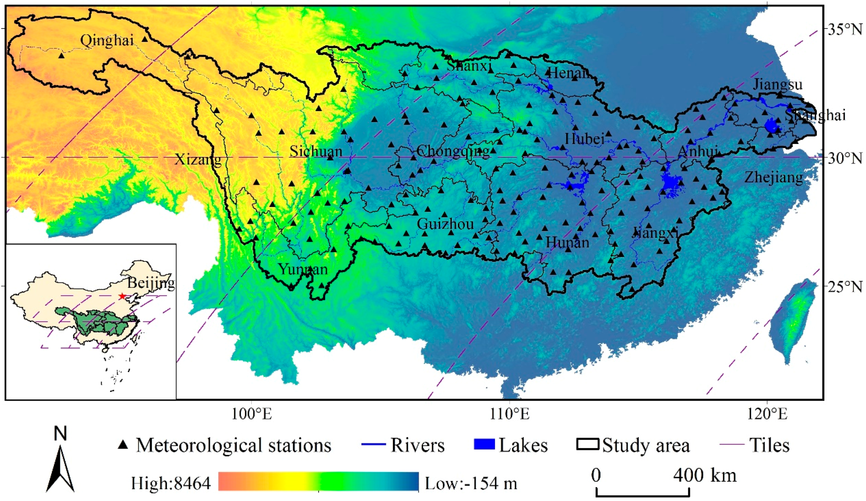
The Yangtze River is in southern China with a drainage area of 1.8 × 10⁶ km2 (24°30′–35°45′ N, 90°33′–122°25′ E), who originates in the Tibetan Plateau and eastward flowing into the East China Sea (Figure 1). YRB covers 14 provinces in southern China. This basin built many water conservation facilities, such as the Three Gorges Hydropower Station. The degree of development varies widely from various regions, with upstream poverty and downstream rich, generally. Serious floods and droughts frequently occur in the middle and lower reaches, resulting in massive human deaths and economic losses. Remote sensing data can be used to observe temporal and spatial variation of surface water for YRB.
2.2. MODIS Products
MOD09A1 (approximately 500 m spatial resolution) provides surface reflectance bands 1–7 for every eight days. It also provides State QA Descriptions data which contains MOD35 cloud/snow/ice flag, land/water flag and cloud shadow. So far, the MOD09A1 product has been used by some researchers to identify surface water information [11,25].
MOD13Q1 (approximately 250 m spatial resolution) is mainly designed to observe changes in vegetation by NDVI and Enhanced Vegetation Index (EVI), as well as provides the auxiliary red, near-infrared, blue and mid-infrared bands, corresponding to Bands 1, 2, 3 and 7, respectively. Also, it provides pixel reliability summary QA, VI Quality detailed QA and the composite days of the year.
The 5th versions of MOD44W products are only one image of the global surface water, and the spatial resolution is 250 m. It has been proven to be reliable and can be used as the basis of sample collection [26].
Seven different tiles (including h25v05, h26v05, h27v05, h28v05, h26v06, h27v06 and h28v06) are required to cover the entire YRB (Figure 1). All images of the 7 tiles for MOD09A1 and MOD13Q1 products, from the 49th day of 2000 to the 257th day of 2016, were downloaded from https://ladsweb.modaps.eosdis.nasa.gov, with a total of 5334 and 2674 images for MOD09A1 and MOD13Q1, respectively. Noteworthy, they are both selected from the 6th versions of MODIS products which is proven to be better than the previous data based on the study results of Zhang et al. [27].
2.3. Ancillary Data
Some ancillary data is needed to collect for classification results correction, accuracy validation and analysis of water changes.
2.3.1. Result Correction Data
Because of external conditions and own shortcomings (such as topographic shading, clouds, ice, snow, cloud shadows and instrument failure), observations from remote sensing satellites can lead to poor observational quality. For MOD09A1 and MOD13Q1, snow, ice, cloud, cloud shadow is available from their QA data (Section 2.2). In addition, digital elevation model (DEM) data with 30 m resolution was downloaded from Geospatial Data Cloud (http://www.gscloud.cn/sources) and processed it into the slope data for this study. It was resampled to 250 m and 500 m for removing terrain shadows.
2.3.2. Accuracy Validation Data
It is necessary to compare the simulation results of the same time in the same area with higher-resolution images such as Landsat for actual case verification. The water extent of Poyang Lake and Dongting Lake varies dramatically, which is easily to be misclassified. Therefore, the simulation results of two lakes can reflect the accuracy of the whole results to a large extent. Some Landsat images of Poyang Lake and Dongting Lake, including the wet and dry season (Section 4.1), were used for accuracy validation. These images are downloaded from the USGS archive (https://earthexplorer.usgs.gov/). This study uses the NDWI to initially extract water bodies and manually corrects them to obtain 30m resolution water body maps. The results were also resampled to 250 m and 500 m resolution for validation.
2.3.3. Precipitation Data
To explore the relationship between the water extent and precipitation, this study collected daily precipitation data of 190 meteorological stations for 2000–2016 from the China Meteorological Data Sharing System (http://data.cma.cn/). These data are interpolated to get monthly precipitation data with 500 m resolution for study area by inverse distance weight interpolation method.
3. Method
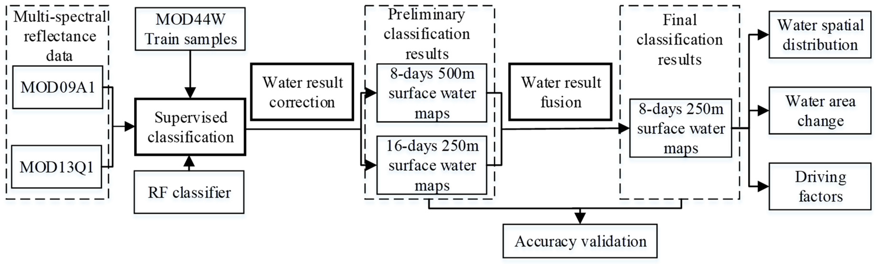
Figure 2 shows the schematic for surface water results acquisition and change analysis. The acquisition of surface water results includes: (1) supervised classification by RF classifier; (2) Water result correction; (3) Water result fusion. Water change analysis includes: (1) water spatial distribution; (2) water area change; (3) driving factors.
3.1. Classification by RF Classifier
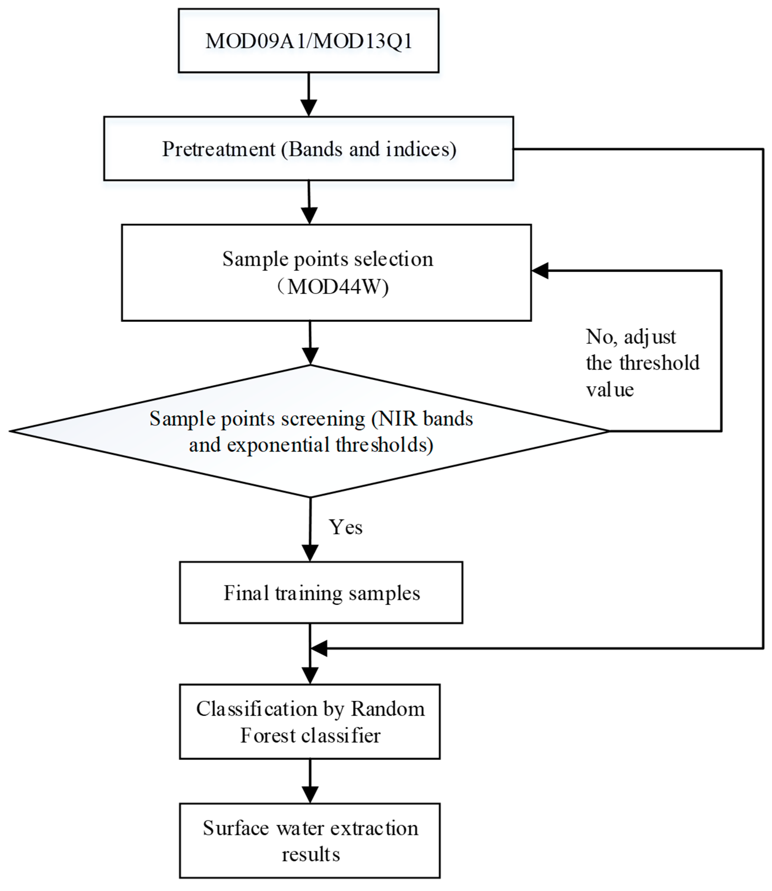
This study uses the random forest (RF) method to extract surface water, which mainly involves three aspects, including RF classifier, feature variable section and sample collection. This specific process can be seen in Figure 3.
3.1.1. Random Forest Classifier
Breiman suggested a classifier in 2001 that is based on statistical theory called RF classifier [28]. This classifier belonging to ensemble learning algorithms is a combination of tree predictors and employs the strategy that a random subset of the predictors is selected to grow a binary tree, where each tree is grown on a bootstrap sample of the training set. The algorithm provides a parameter called out-of-bag (OOB) that is the ratio of samples that have not been used for training, and the out-of-bag error (OOB error) represents the generalization error which can be regarded as the validation result for the model.
Compared with a single decision tree classifier, RF classifier is more robust and has the good generalization ability in the classification process because of the characteristics of multiple trees and repetitive sampling. RFs have been widely used in feature classification [29,30,31], and water extraction is also involved in the recent [10]. In general, RF classifier includes the following several advantages: (a) robust to outliers and noise; (b) efficiently and fast to classify, c) not easily overfitting. In this paper, RF classifier was chosen as the classification method because of its efficient application for long-term serial images.
3.1.2. Feature Variable Section
Feature variable selection is one of the key points of classification. It will have a direct impact on the performance of a classifier since the model of the classifier is expressed by some feature variables. In general, taking as many relevant feature variables as possible is beneficial to modeling. For MOD13Q1 products, four bands (Bands 1/2/3/7) and two indices (NDVI/EVI) were all selected as feature variables. For MOD09A1 products, some indices which are often used to extract surface water are lacking. Therefore, some relevant indices are calculated by the known bands, including NDVI, NDWI and MNDWI. Finally, a total of seven bands (Bands 1–7) and three indices (NDVI/NDWI/MNDWI) are used as feature variables for MOD09A1 products to extract water.
3.1.3. Sample Collection
Determination of samples is required prior to modeling. To make the samples meet representativeness and reliability along with fast and efficient simulation model, the spatial position of sample points should be as uniform as possible while the number of sample points is controllable. The sample points for a tile were collected according to the following: (a) taking the central pixel as a sample point in the 20 × 20 non-water pixels, that is, selecting a non-water sample point per 5000 m (MOD44W with 250 m spatial resolution); (b) taking the central pixel as a sample point in the 6 × 6 water pixels, that is, selecting a water sample point per 1500 m. According to the above-noted procedure, a total of about 50,000 non-water sample points and 15,000 water sample points can be selected for an image, and a total of approximately 500,000 water and non-water sample points are selected.
The surface water extent in different periods is different because of its dynamic characteristics, so the primary samples selected by MOD44W cannot be used directly. To ensure that the water or non-water sample points are completely unmistakable, this study selects the near infrared band and some indices by setting certain thresholds to filter sample points. Taking the h27v06 tile of MOD09A1 data as an example, the thresholds of NDWI and MNDWI are both set to 0.2 and the threshold of NDVI is set to −0.2, as well as the threshold of near infrared is set to 3500 for water sample points, which means that the water sample points that meet NDWI > 0.2 and MNDWI > 0.2 and NDVI < −0.2 and b2 > 3500 are the final water sample points. Correspondingly, the non-water points meeting NDWI < −0.2 and MNDWI < −0.2 and NDVI > 0.2 and b2 < 5000 are the final non-water sample points. For MOD13Q1, the near infrared band and NDVI are considered. Taking h27v06 as an example, water sample points meet NDVI < −0.2 and b2 > 3500, and non-water sample points meet NDVI > 0.2 and b2 < 5000.
3.2. Water Result Correction
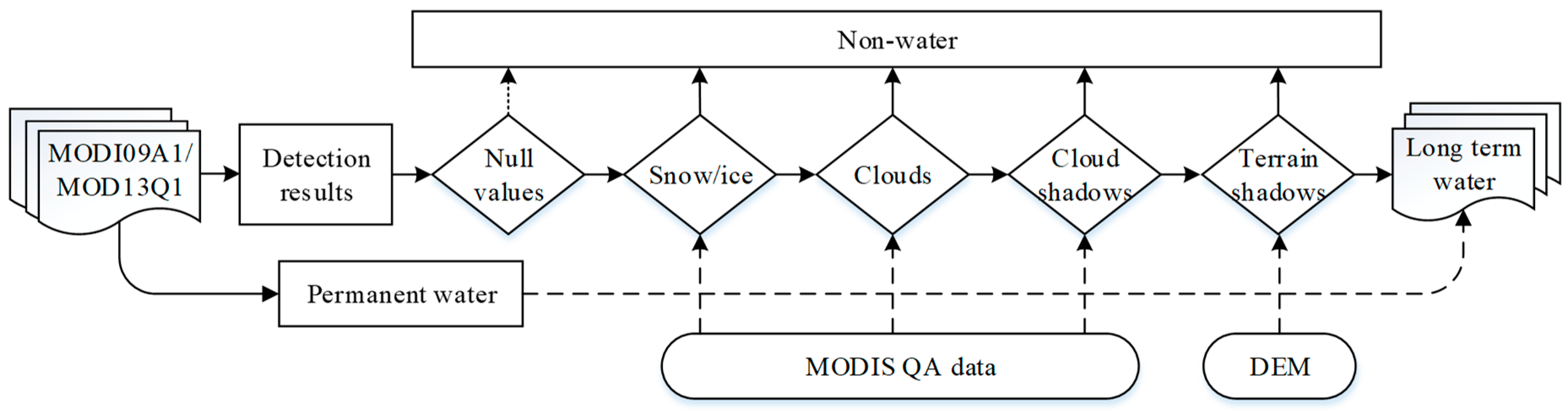
Figure 4 provides the specific process of correction for water extraction results. Clouds, cloud shadows and snow/ice can all be obtained from the QA data of MOD09A1 and MOD13Q1. Terrian shadows can be removed by DEM data.
3.3. The Fusion Method of Water Results
Using the above methods, two sets of surface water results were obtained, with 8 days 500 m resolution and 16 days 250 m resolution, respectively. However, the 500-m resolution is rough enough that some water information does not show up, and a 16-day interval cannot be a good show for hydrological process, especially the flood process. Therefore, this study intends to use these two sets of data to obtain more accurate surface water products by a fusion method. The purpose is to combine the advantages of two sets of products to obtain higher-resolution and more accurate water products. At last, the surface water results are 8-day 250-m resolution.
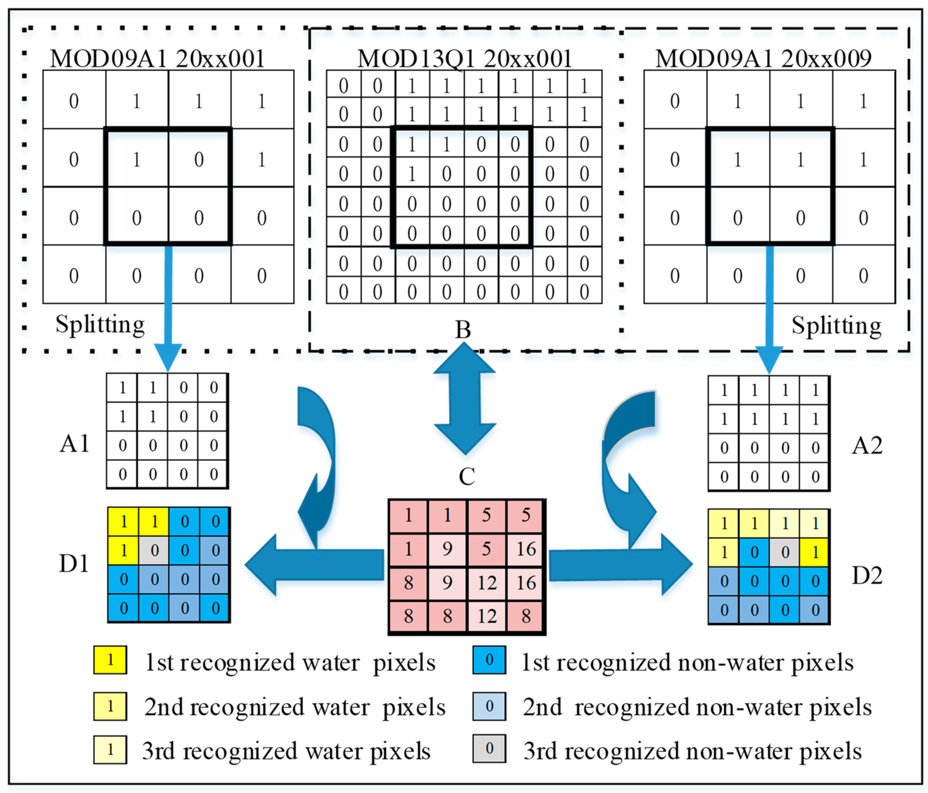
The water result fusion process is shown in Figure 5. A1 and A2 are the pixels of 500 m water extraction results from MOD09A1 for 20xx001th day and 20xx009th day, and B is the pixel of 250 m water extraction results from MOD13Q1 for 20xx001th day. C is the corresponding production date for each pixel of B, which is the auxiliary band of MOD13Q1. The value range of C is 1–16 for 20xx001th day, where 1–8 and 9–16 is corresponding to 20xx001th day and 20xx009th day for MOD09A1, respectively. The values of A1, A2 and B can only be 0 or 1, where 0 represents non-water and 1 represents water. A1 and A2 are both resampled directly into 250 m, and one pixel is split into four, so their number of rows and columns is the same with B.
Three steps to determine the final values of all A1 pixels: first step, if 1 ≤ C < 9, A1 is replaced by B; second step, if 9 ≤ C < 17 and A1 = B, the value of A1 does not change; last step, if 9 ≤ C < 17 and A1 is not equal to B, the gradient of A1 and B can be calculated by taking a window of 3 × 3 pixels:
where i is the location of A1, A2 and B; t is the location of its neighboring pixels; T is the total number of surrounding pixels in the total window (here is 8); dx is the distance between two pixels and dy is the difference between two pixel values (the value of dy is 0 or ±1).
Assuming the distance between adjacent pixels is 1, the value of dx can be only 1 or √2. Therefore, if , the value of A1 does not change, else A1 is replaced by B.
These 3 steps correspond to the order in which the pixels are recognized. It can also be expressed as the following Equation (2).
where D1 is the pixel of fusion results for 20xx001th day.
Based on the above steps, judging the final value for each pixel, the surface water map for the 20xx001th day can be obtained. Likewise, using A2, B and C, the surface water map for the 20xx009th day can also be produced (Equation (3)).
Similarly, using all the pixel date data of MOD13Q1 product from 2000049–2016257 days, we can get 762 fused result maps.
3.4. Accuracy Validation of Water Results
Accuracy validation is essential for simulation results. For RF classifier, the OOB error is a good validation value that can replace the test sample. Therefore, test samples were not selected in this paper. The accuracy of the simulation results can be determined by comparing them with the water extraction results from some higher-resolution images which can be seen as accurate. Poyang Lake and Dongting Lake are the two most typical seasonal lakes in the YRB, which are most likely to be misclassified. Some Landsat images of Poyang Lake and Dongting Lake, including the wet and dry season (Section 4.1), were used for accuracy validation. These images are downloaded from the USGS archive (https://earthexplorer.usgs.gov/). This study uses the NDWI to initially extract water bodies and manually corrects them to obtain 30 m resolution water body maps. The results were also resampled to 250 m and 500 m resolution for validation.
3.5. Dynamic Change Analysis of Surface Water
3.5.1. Water Inundation Frequency Mapping
For water classification maps, we can count the water inundation frequency (p) for each pixel in the total time series by multi-map overlay. Its formula can be expressed as follows:
where N represents the number of long-term serial water maps; i represents the corresponding ith water map; represents the corresponding pixel value of the ith water map, where 1 is water and 0 is non-water.
3.5.2. Water Type Classification
There are obvious differences in variation characteristics between seasonal water and permanent water [9,32]. A threshold was set to distinguish this seasonal and permanent water. Considering the surface water characteristic of the study area, the threshold is set to 0.5, which means that more than 50% of the total number of occurrences is considered to be permanent water and the other part is seasonal water.
4. Results
4.1. Accuracy Evaluation of Water Results
The RF classifier needs to determine two parameters including classification trees and the number of feature variables. In this paper, all selected feature variables are applied to simulation. Therefore, the determination of the number of trees is necessary. Figure 6 shows some 10 simulation examples with the relationship between the number of trees and the OOB error for the tile h27v06. Obviously, the OOB error of all examples is less than 0.05 when the number of trees exceeds 20. In this study, the number of simulation is set to 100 times, and the simulation result with the smallest OOB error is used for classification.
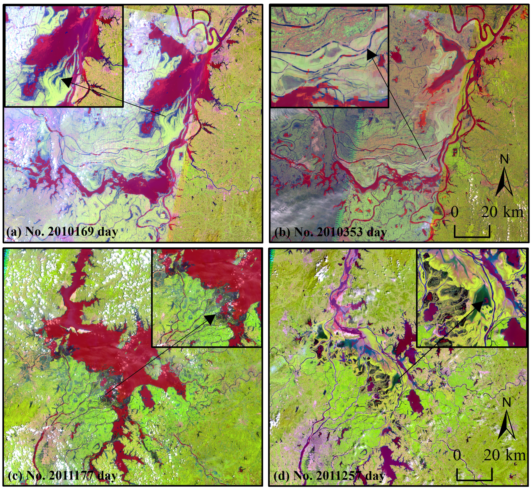
The water extraction results in both wet and dry seasons of Dongting Lake and Poyang Lake are shown in Figure 7. The extraction results are both satisfying in the dry or wet season.
Table 1 summarizes the accuracy of water extraction results, including user’s accuracy (UA), producer’s accuracy (PA), overall accuracy (OA), Kappa coefficient (KC). The values of OA and UA are all greater than 0.9. The values of PA are relatively low with generally greater than 0.8 in the wet season, but the values are between 0.65 and 0.8 in the dry season, which proves the proportion of omission water pixels is relatively large especially in the dry season. Kappa coefficient is generally greater than 0.8, and the values of the wet season are larger than that of the dry season. Overall, the accuracy of extraction results is satisfying for both dry and wet seasons.
4.2. Surface Water Spatial Distribution of the YRB
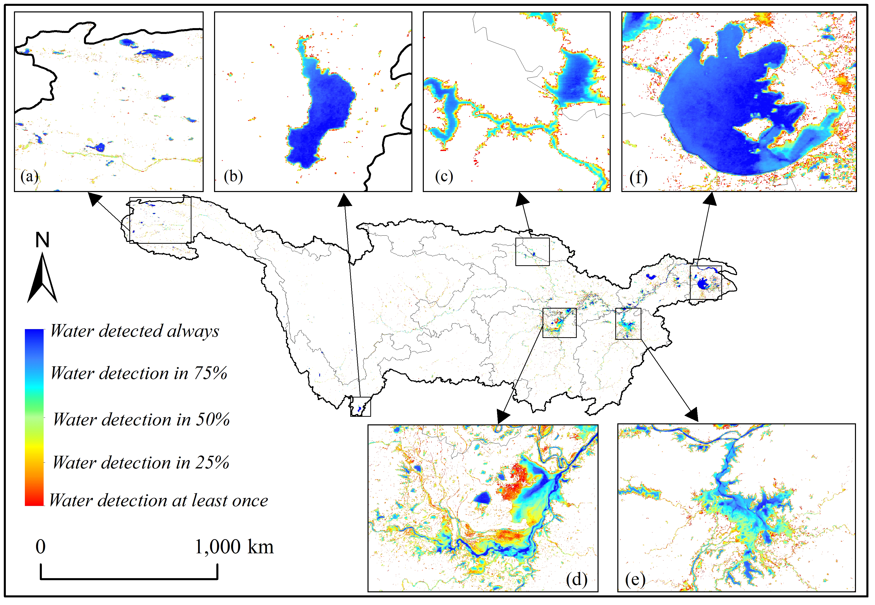
In this paper, the products are eventually obtained and visualized by 762 remote sensing images of water and non-water. Figure 8 illustrates the superimposed map of all surface water extraction results, which can be used to express the overall situation of water extraction results and water inundation frequency for each pixel. The maximum area that surface water inundation at least once from 2000 to 2016 is 48.53 × 10³ km2, which accounts for 2.70% of the total area of the basin. The surface water in different areas of the YRB varies largely. A wide range of surface water bodies, such as lakes and large reservoirs, are mainly distributed among the middle and lower reaches of the basin. Six typical lakes and reservoirs were selected from downstream to upstream of YRB (Figure 8). Poyang Lake and Dongting Lake have significant seasonal variations, and the remaining four are relatively small.
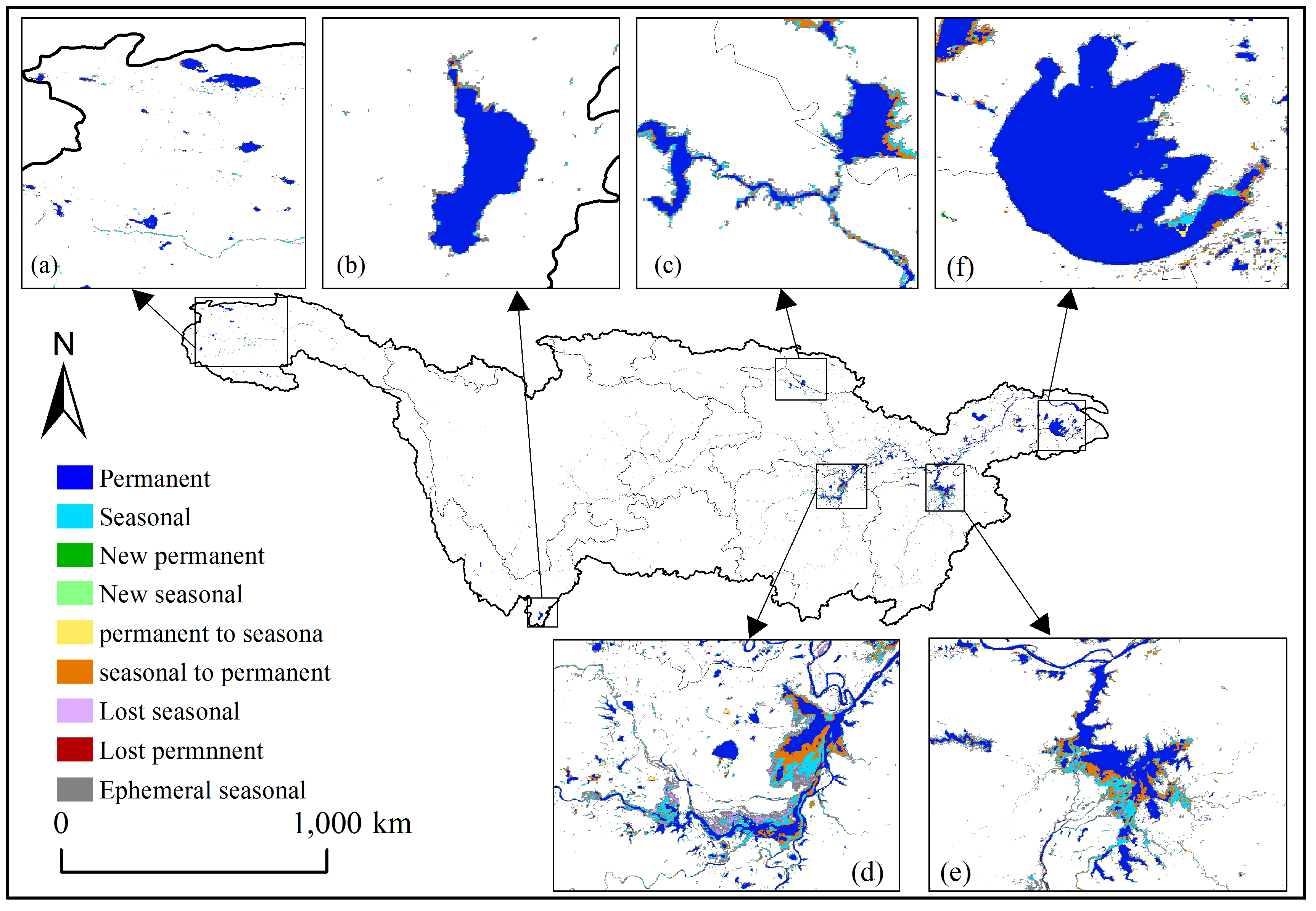
According to the water type classification standard (Section 3.5), the seasonal and permanent water area of YRB were 20.51 × 10³ km2 and 28.01 × 10³ km2, respectively. Further, this study counts the changes in permanent and seasonal water which are calculated through the results of 2011–2015 minus 2001–2005′s (Figure 9). The season and permanent water of Dianchi Lake and source of the Yangtze River hardly changed. Part of the seasonal water transforms into permanent water in Danjiangkou Reservoir, which is affected by the South-North Water Transfer Project in 2014. Permanent and seasonal water in the southeast of Taihu Lake change greatly, mainly including seasonal to permanent (S2P), permanent to season (P2S) and lost seasonal (LS) water. Spatial changes of the permanent and seasonal water are significant in Poyang Lake and Dongting Lake. Seasonal to permanent (S2P) and lost seasonal (LS) water are main change in Dongting Lake and Poyang Lake. Furthermore, ephemeral seasonal water with the area of 10.61 × 10³ km2 in the YRB accounts for relatively large, especially in the Poyang Lake and Dongting Lake.
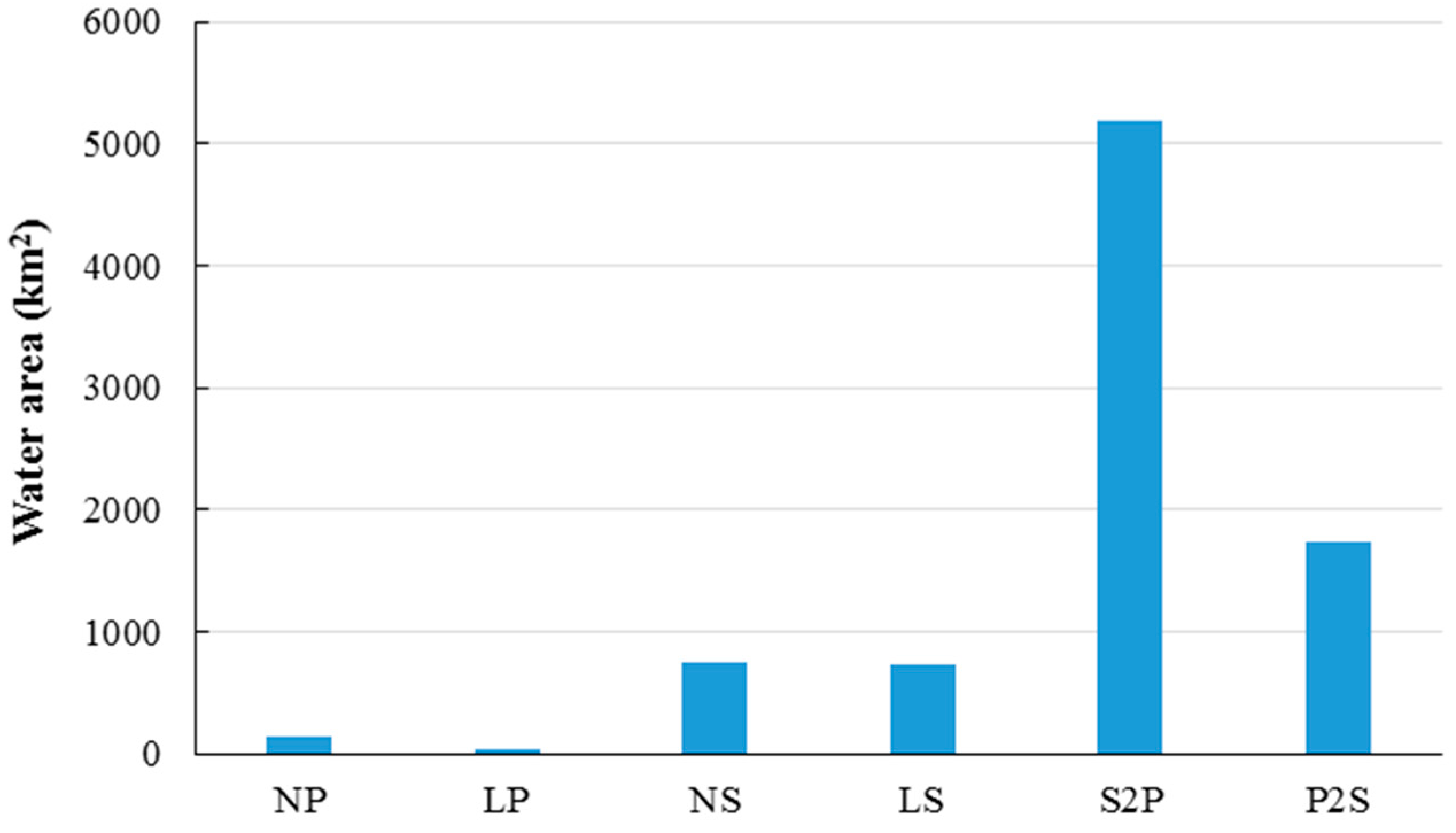
The area of changed seasonal and permanent (including NP, LP, NS, LS, S2P and P2S) water is calculated (Figure 10). In general, the seasonal water area decreased by 3450 km2, and the permanent water area increased by 3565 km2.
4.3. Surface Water Area Change of the YRB
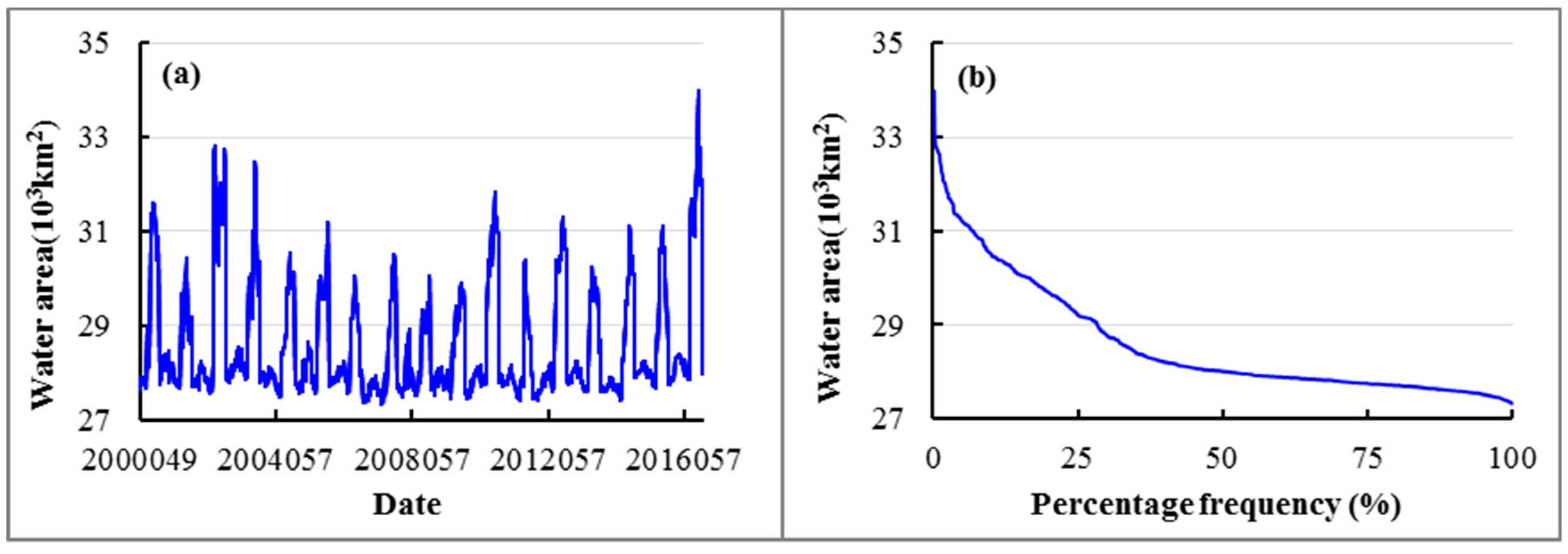
The surface water area is calculated every 8 days during 2000–2016 in the YRB. According to Figure 11a, the surface water area of the YRB shows obvious annual cyclical changes, with larger in summers and smaller in winters. The largest water area occurred in day 2016201 with a corresponding area of 33.99 × 10³ km2, and the smallest water area occurred in day 2007097 with an area of 27.34 × 10³ km2. 762 water area values are sorted by size, and their percentage frequencies are calculated (Figure 11b). The results show that the values of ranked 5%, 25%, 50%, 75% and 95% were about 31.20 × 10³, 29.20 × 10³, 28.00 × 10³, 27.70 × 10³ and 27.50 × 10³ km2, respectively.
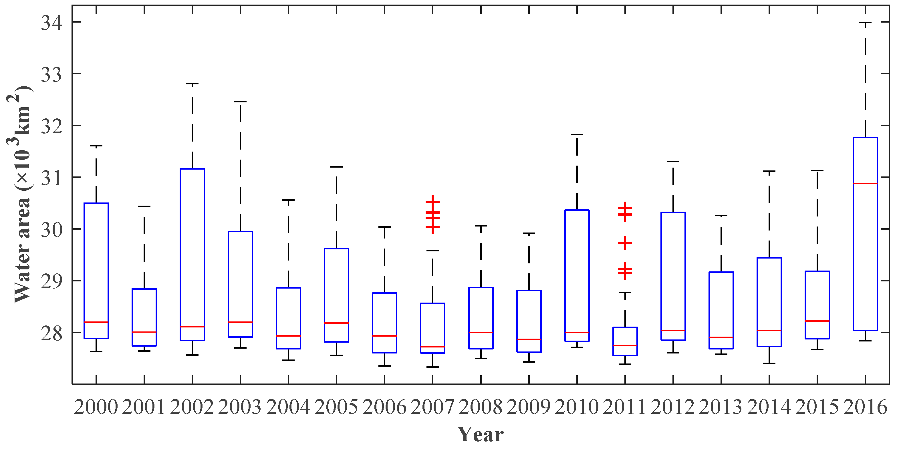
The peak, Median, and valley values of the water area for each year are counted (Figure 12). The most water year is 2016, which the peak, median and valley values of the water area are all the largest in 17 years, 33.99 × 10³, 30.88 × 10³ and 27.84 × 10³ km2, respectively. Other years with a large amount of water are 2002, 2003 and 2015. The year of less water includes 2001, 2006, 2007, 2008, 2009 and 2011. The minimum peak, median and valley values occurred in 2009 with water area of 29.91 × 10³ km2, 2011 with water area of 28.04 × 10³ km2, 2007 with water area of 27.34 × 10³ km2, respectively. In addition, the years (2007 and 2011) show several abnormal values and are relatively dry, which indicators the surface water area in most of these years is small.
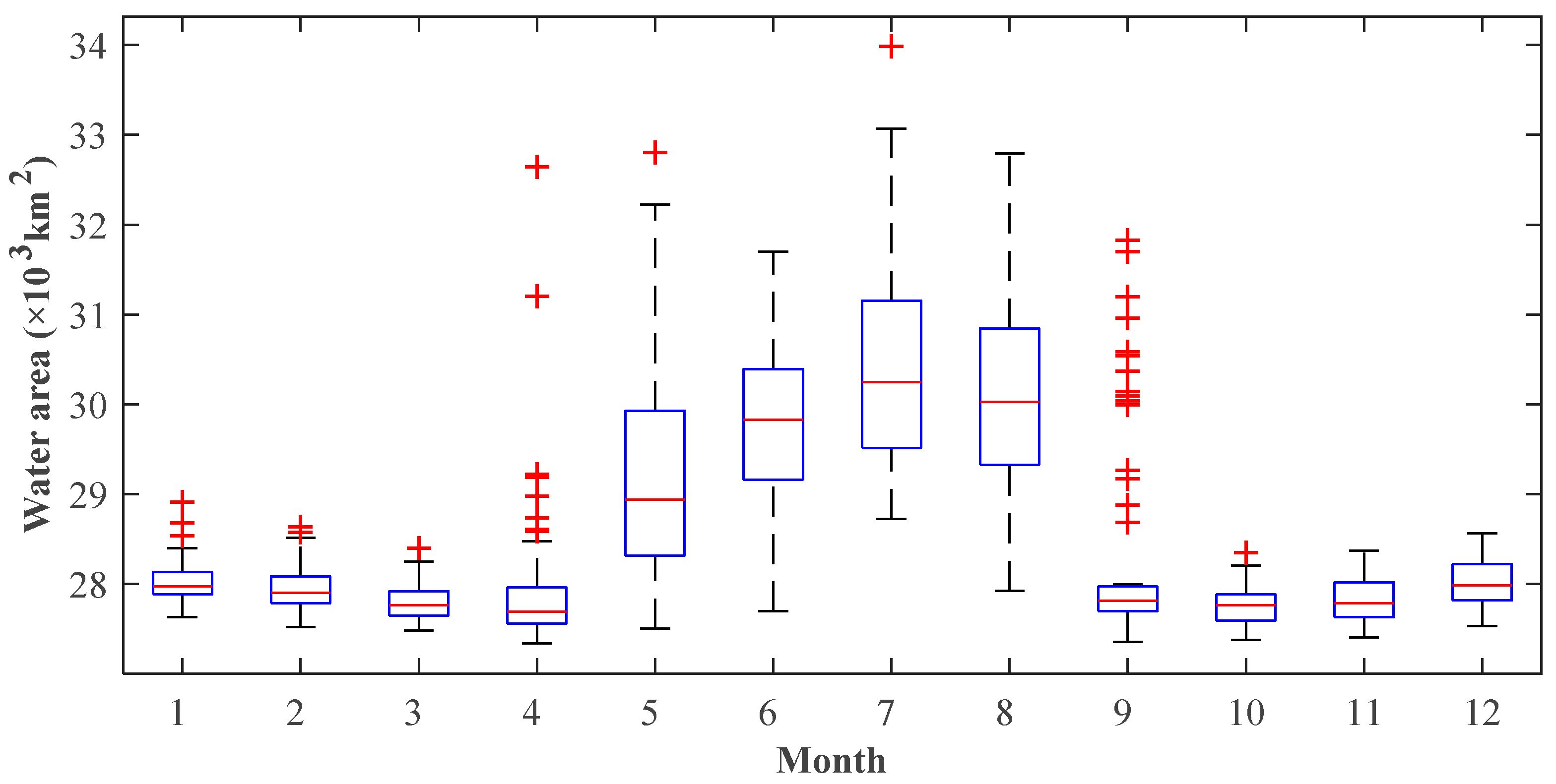
Surface water area varies greatly in different months (Figure 13). The peak, median and valley values of the water area are obviously larger from May to September, and their largest values all occurred in July with water area of 33.99 × 10³, 30.21 × 10³ and 28.72 × 10³ km2, respectively. April and October are special. Their maximum water area is large basically as same as May–September, and the minimum water area is small the same as other months.
4.4. Surface Water Extent Changes Due to Precipitation
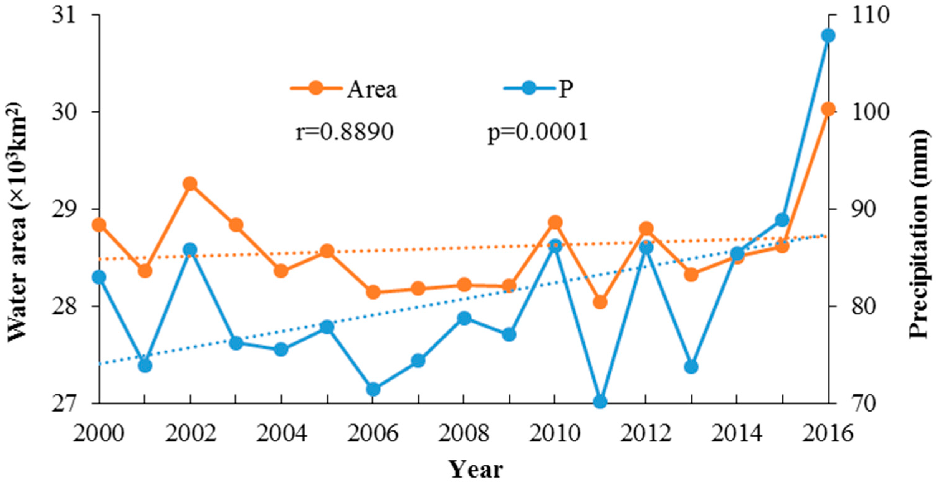
Precipitation plays a critical role in water area for the basin, especially for these lakes such as Poyang Lake and Dongting Lake. This study counts the correlation between water area and precipitation from 2000 to 2016 for YBR (Figure 14). The results showed a significant correlation between them (p = 0.0001 < 0.05), and the correlation coefficient is 0.9076. In addition, Precipitation and water area are both increasing from 2000 to 2016, especially from 2011 to 2016. Due to incomplete data in 2000 and 2016, and 2016 is a typical flood year in YRB. If we only consider 2001 to 2015, the results show that precipitation increases slowly, and water area has no obvious trend.
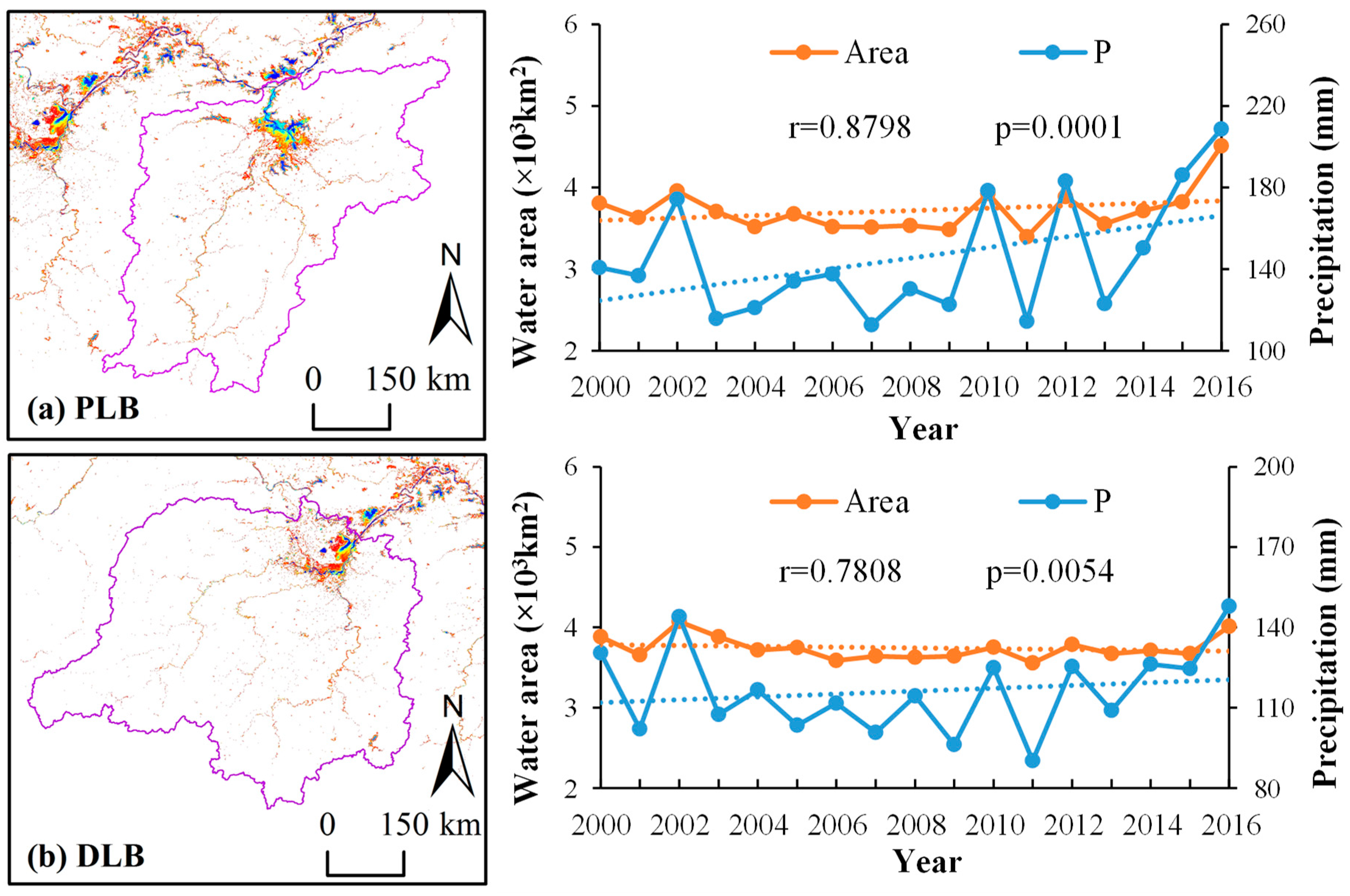
Poyang Lake and Dongting Lake are the two most typical lakes affected significantly by seasonal precipitation (Figure 9). The study calculated the correlation between precipitation and water area in the two lake basins (Figure 15). The correlation between precipitation and water area is significant (p = 0.0001 < 0.05) and the correlation coefficient is 0.8798 in Poyang Lake Basin (PLB). Similarly, the relationship of them in Dongting Lake Basin (DLB) is also significant (p = 0.0054 < 0.05), with a correlation coefficient of 0.7808. In addition, the water area of PLB is increasing while DLB’s is decreasing although the precipitation of both is increasing from 2000 to 2016. It indicates that the surface water bodies of the DLB have been seriously affected by human activities in 2000–2016 period.
5. Discussion
5.1. Water Extraction Method Performance
Some similar studies have been proposed [13,14], but few have involved a research area with more than 1×10⁵ km2. This is a major difficulty in the work of this study. In general, some past studies are limited to classification methods and band information applications [11], and some exhibit defects to the spatiotemporal resolution of the results [10,12].
To make full use of the information of multiple bands and obtain more accurate long-term serial and large-scale surface water bodies, this paper used the RF classifier, many sample points and multi-feature variables to construct a long-term serial surface water extraction method. Although the classification method used in this study is not original, the method has been specifically improved to obtain reliable surface water bodies. A total of 5334 images for MOD09A1 and 2674 images for MOD13Q1 is involved in the classification.
In addition, the process of water result correction also made good use of related band information and other ancillary information and obtained better water results. Compared to the preliminary classification process, water correction process may be more critical to the results. It is worth mentioning that a data fusion method based on the date information of the pixel production is presented for obtaining the water results with higher spatiotemporal resolution in this study. Eventually, 762 surface water distribution maps with eight-day and 250 m spatiotemporal resolution are produced.
Moreover, the fusion method for improving the spatiotemporal resolution of long-term serial results can be introduced to other remote sensing data applications.
5.2. Flood Analysis Using the Products
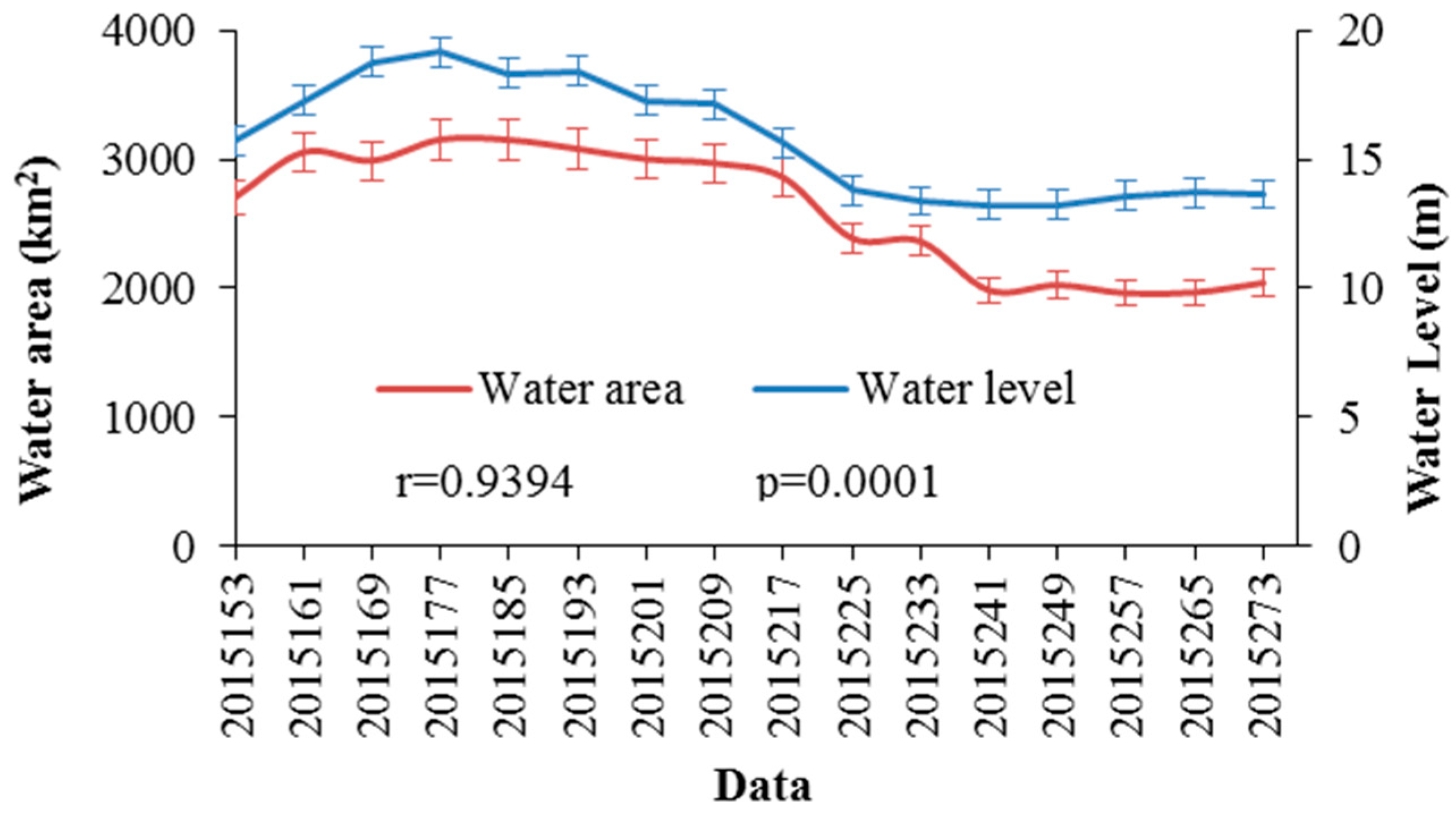
Water level runoff curve is one of the most important means to assess and forecast floods. However, due to flood fluctuations and changes in return water and other effects, it is often unstable for the water level runoff curve reflecting the flood [33]. The water extracted by remote sensing data can intuitively demonstrate flooding range. Figure 16 showed the relationship between water area and water level at Poyang Lake during the 2015 wet season. Their correlation is very high (r = 0.9394) and the peak is also consistent. Obviously, the products can better reflect the flood process.
In future, we will further to explore the application of this data in the flood process of other lakes and rivers in the study area. Moreover, as a disaster event, floods can also be used to explore the impact of floods on some things, such as economic losses and crop damage [34]. Remote sensing data with high temporal resolution can be used as basic data for determining the extent of floods for disaster result analysis.
5.3. Surface Water Characteristics of the YRB in 2000–2016
The surface water in the YRB is mainly distributed in several important lakes, reservoirs, and rivers. The surface water inundation frequency and the changes in permanent and seasonal water indicate a huge difference in different lakes or rivers in the YRB (Figure 8 and Figure 9). The water extents of Poyang Lake and Dongting Lake change greatly, and the changes in Taihu Lake and Dianchi Lake are very small. This first reason is because the water from the upper reaches of the lake is different. More importantly, Poyang Lake and Dongting Lake are directly connected to the Yangtze River. This similar conclusion can be found in in the research of Wang et al. [35].
Precipitation is the most important factor causing changes in water area for the whole basin. Although affected by the inflow and outflow of the Yangtze River, Poyang Lake and Dongting Lake also meet this relationship, mainly because wet season and dry season are relatively consistent in the whole basin. Apart from precipitation, some other factors can also affect changes in the surface water, such as human activities. Given the slope of the precipitation is greater than the slope of the water area (Figure 14), they have reduced the water area to a certain extent.
Water conservation facilities have a great impact on the change in surface water. Three Gorges Dam has a significant impact on the downstream lakes and rivers, which reduced peak and slightly increased low discharges [36]. It is consistent with the conclusion of this study that the seasonal water reduced, and the permanent water increased. The water storage capacity of the Danjiangkou Reservoir in the middle line of the South-to-North Water Diversion Project has increased since 2014. Farmland reclamation, urbanization and artificial breeding are also important human activities, typical examples are Poyang Lake, Dongting Lake and Taihu Lake. This will be the next work to be carried out.
5.4. Issues and Uncertainties
This study attemped to acquire continuous long-term serial water maps by remote sensing data in the study area. However, some issues still exist, and further work needs to be carried out. Although RF classifier is an efficient machine learning method, the classification results also exist partial misclassification and misclassification of water bodies. Some small rivers have not been extracted in Figure 8a,b. Figure 8a,c show that the simulation results are hardly affected by thin clouds. Figure 8d shows that part of the water bodies containing impurities is not extracted. These indicate: (1) the extraction results are better for the wet season; (2) clouds have a great impact on water extraction, but the impact is small after treatment, especially for thin clouds; (3) water extraction accuracy is affected by various kinds of impurities, such as algae and sediment. Recently, some efficient and intelligent water extraction methods such as SMDPSO by Jia et al. and C/M by Tarpanelli et al. have been proposed to better acquire water bodies [37,38].
Sample selection and data correction are also critical. The quality and number of sample points will have a profound influence on the results [39]. This study selected approximately 500,000 sample points and considered spatial difference in the sample points by uniformly sampling. Some wrongly sampled points must exist, but the wrong use of a small number of sample points will not have a significant impact on the results. Water result correction mainly refers to the research of Pekel et al. and Khandelwal et al. [10,13]. This paper does not make specific detailed introduction to the correction of each tile, but corrected results are proved to be reliable by verification. Furthermore, a feasible fusion method has been proposed to combine these two sets of water results. This method mainly considers the temporal relationship of two sets of data and establishes a mathematical function based on spatial autocorrelation to determine the fused results. Fusion results eliminated some misclassification water pixels and are proved to have higher precision than before (Table 1). Visibility, it applies well to the field of remote sensing. However, the problem is the fusion results eliminated some real water pixels. Next, we are also going to try to improve the function for better integration of results.
Validation of the water body result is not completely sufficient for only a few typical cases. Some comparisons should exist with other data results. Considering current available results from Pekel’s research still have some problems for the study area [9], this study does not make specific comparisons. Although no suitable water dynamic extent data of the study area has been found yet, some other data from satellite altimetry, Gravity Recovery and Climate Experiment (GRACE) and Global Land Data Assimilation System (GLDAS), etc. can be also used as comparisons and validation [25,38,40]. This will be the work that we will continue to carry out in the next step, which may better illustrate the water resources issue in the research area.
6. Conclusions
Surface water plays an important role in the allocation of water resources. Persistent surface water bodies mapped with short time intervals and long time series are valuable for flood, drought, and water resource management in the YRB. In this study, 762 continuous surface water dynamic maps of the YBR from 2000 to 2016 were obtained by using RF method and MODIS data. Two highlights can be summarized for this study below.
First, this study constructed an approach for surface water automatic extraction based on the RF classifier. Moreover, a data fusion method was proposed to obtain more accurate water extraction results with higher spatiotemporal resolution. This method is innovative, and it can be used to acquire surface water maps with greater scale or higher spatiotemporal resolution in the future. It may also be used for the remote sensing classification of other features such as vegetation to some extent.
Second, quantitative analysis is conducted to assess dynamic changes in 2000–2016 for surface water of the study area based on these products. This result shows that:
- (1)
- The largest water area is 33.99 × 10³ km2 occurred in day 2016201, and the smallest water area is 27.34 × 10³ km2 occurred in day 2007097. The maximum area of surface water inundation at least once in the YBR from 2000 to 2016 is 48.53 × 10³ km2, and seasonal and permanent water areas are 20.51 × 10³ km2 and 28.01 × 10³ km2.
- (2)
- Surface water area is increasing in the YRB. Permanent water body rises and seasonal water body drops. The seasonal water area decreased by 3450 km2, and the permanent water area increased by 3565 km2 in 2001–2015.
- (3)
- Precipitation plays an important role in the variation of surface water area in the YRB. Precipitation and water area both showed a certain increased trend, but the increase in precipitation is more pronounced than the water area for the entire basin. Similar conclusions can be obtained for the PLB and DLB. Human activities have reduced the water area to some extent for this study from 2000 to 2016.
This research puts forward a better approach to explore the dynamic changes of surface water bodies, and the quantitative results can provide some basis for the relevant departments to formulate the water resource management policy for the study area.
Author Contributions
This paper was conceived through P.R. and W.J., and the main work was also done through them. In addition, Y.H. provided some data and many suggestions for this paper. Z.C. and K.J. also provided some very key suggestions in the manuscript writing section.
Funding
This research was funded by the National Key Research and Development Program of China (2016YFC0503002) and the National Natural Science Foundation of China (41571077 and 40701172).
Conflicts of Interest
The authors declare no conflict of interest.
References
- Downing, J.A.; Prairie, Y.T.; Cole, J.J.; Duarte, C.M.; Tranvik, L.J.; Striegl, R.G.; McDowell, W.H.; Kortelainen, P.; Caraco, N.F.; Melack, J.M.; et al. The global abundance and size distribution of lakes, ponds, and impoundments. Limnol. Oceanogr. 2006, 51, 2388–2397. [Google Scholar] [CrossRef] [Green Version]
- Prigent, C.; Papa, F.; Aires, F.; Rossow, W.B.; Matthews, E. Global inundation dynamics inferred from multiple satellite observations, 1993–2000. J. Geophys. Res. 2007, 112. [Google Scholar] [CrossRef] [Green Version]
- Pham-Duc, B.; Prigent, C.; Aires, F.; Papa, F. Comparisons of Global Terrestrial Surface Water Datasets over 15 Years. J. Hydrometeorol. 2017, 18, 993–1007. [Google Scholar] [CrossRef]
- Vorosmarty, C.J. Global Water Resources: Vulnerability from Climate Change and Population Growth. Science 2000, 289, 284–288. [Google Scholar] [CrossRef] [PubMed]
- Vörösmarty, C.J.; McIntyre, P.B.; Gessner, M.O.; Dudgeon, D.; Prusevich, A.; Green, P.; Glidden, S.; Bunn, S.E.; Sullivan, C.A.; Liermann, C.R.; et al. Global threats to human water security and river biodiversity. Nature 2010, 467, 555–561. [Google Scholar] [CrossRef] [PubMed] [Green Version]
- Kanakoudis, V.; Papadopoulou, A.; Tsitsifli, S.; Curk, B.C.; Karleusa, B.; Matic, B.; Altran, E.; Banovec, P. Policy recommendation for drinking water supply cross-border networking in the Adriatic region. J. Water Supply Res. Technol. AQUA 2017, 66, 489–508. [Google Scholar] [CrossRef]
- Kanakoudis, V.; Tsitsifli, S.; Papadopoulou, A.; Curk, B.C.; Karleusa, B. Estimating the Water Resources Vulnerability Index in the Adriatic Sea Region. Procedia Eng. 2016, 162, 476–485. [Google Scholar] [CrossRef]
- Kanakoudis, V.; Tsitsifli, S.; Papadopoulou, A.; Cencur Curk, B.; Karleusa, B. Water resources vulnerability assessment in the Adriatic Sea region: The case of Corfu Island. Environ. Sci. Pollut. Res. 2017, 24, 20173–20186. [Google Scholar] [CrossRef] [PubMed]
- Pekel, J.-F.; Cottam, A.; Gorelick, N.; Belward, A.S. High-resolution mapping of global surface water and its long-term changes. Nature 2016, 540, 418–422. [Google Scholar] [CrossRef] [PubMed]
- Deng, Y.; Jiang, W.; Tang, Z.; Li, J.; Lv, J.; Chen, Z.; Jia, K. Spatio-Temporal Change of Lake Water Extent in Wuhan Urban Agglomeration Based on Landsat Images from 1987 to 2015. Remote Sens. 2017, 9, 270. [Google Scholar] [CrossRef]
- Ogilvie, A.; Belaud, G.; Delenne, C.; Bailly, J.-S.; Bader, J.-C.; Oleksiak, A.; Ferry, L.; Martin, D. Decadal monitoring of the Niger Inner Delta flood dynamics using MODIS optical data. J. Hydrol. 2015, 523, 368–383. [Google Scholar] [CrossRef]
- Mueller, N.; Lewis, A.; Roberts, D.; Ring, S.; Melrose, R.; Sixsmith, J.; Lymburner, L.; McIntyre, A.; Tan, P.; Curnow, S.; et al. Water observations from space: Mapping surface water from 25 years of Landsat imagery across Australia. Remote Sens. Environ. 2016, 174, 341–352. [Google Scholar] [CrossRef]
- Khandelwal, A.; Karpatne, A.; Marlier, M.E.; Kim, J.; Lettenmaier, D.P.; Kumar, V. An approach for global monitoring of surface water extent variations in reservoirs using MODIS data. Remote Sens. Environ. 2017, 202, 113–128. [Google Scholar] [CrossRef]
- Tulbure, M.G.; Broich, M.; Stehman, S.V.; Kommareddy, A. Surface water extent dynamics from three decades of seasonally continuous Landsat time series at subcontinental scale in a semi-arid region. Remote Sens. Environ. 2016, 178, 142–157. [Google Scholar] [CrossRef]
- Donchyts, G.; Baart, F.; Winsemius, H.; Gorelick, N.; Kwadijk, J.; van de Giesen, N. Earth’s surface water change over the past 30 years. Nat. Clim. Chang. 2016, 6, 810–813. [Google Scholar] [CrossRef]
- Feng, L.; Hu, C.; Chen, X.; Cai, X.; Tian, L.; Gan, W. Assessment of inundation changes of Poyang Lake using MODIS observations between 2000 and 2010. Remote Sens. Environ. 2012, 121, 80–92. [Google Scholar] [CrossRef]
- Xu, H. Modification of normalised difference water index (NDWI) to enhance open water features in remotely sensed imagery. Int. J. Remote Sens. 2006, 27, 3025–3033. [Google Scholar] [CrossRef]
- Sakamoto, T.; Van Nguyen, N.; Kotera, A.; Ohno, H.; Ishitsuka, N.; Yokozawa, M. Detecting temporal changes in the extent of annual flooding within the Cambodia and the Vietnamese Mekong Delta from MODIS time-series imagery. Remote Sens. Environ. 2007, 109, 295–313. [Google Scholar] [CrossRef]
- Jiang, W.; Rao, P.; Cao, R.; Tang, Z.; Chen, K. Comparative evaluation of geological disaster susceptibility using multi-regression methods and spatial accuracy validation. J. Geogr. Sci. 2017, 27, 439–462. [Google Scholar] [CrossRef]
- Rodriguez-Galiano, V.F.; Chica-Olmo, M.; Abarca-Hernandez, F.; Atkinson, P.M.; Jeganathan, C. Random Forest classification of Mediterranean land cover using multi-seasonal imagery and multi-seasonal texture. Remote Sens. Environ. 2012, 121, 93–107. [Google Scholar] [CrossRef]
- Pal, M. Random forest classifier for remote sensing classification. Int. J. Remote Sens. 2005, 26, 217–222. [Google Scholar] [CrossRef]
- Nitze, I.; Barrett, B.; Cawkwell, F. Temporal optimisation of image acquisition for land cover classification with Random Forest and MODIS time-series. Int. J. Appl. Earth Obs. Geoinf. 2015, 34, 136–146. [Google Scholar] [CrossRef]
- Xu, K.; Chen, Z.; Zhao, Y.; Wang, Z.; Zhang, J.; Hayashi, S.; Murakami, S.; Watanabe, M. Simulated sediment flux during 1998 big-flood of the Yangtze (Changjiang) River, China. J. Hydrol. 2005, 313, 221–233. [Google Scholar] [CrossRef]
- Lu, E.; Liu, S.; Luo, Y.; Zhao, W.; Li, H.; Chen, H.; Zeng, Y.; Liu, P.; Wang, X.; Higgins, R.W.; et al. The atmospheric anomalies associated with the drought over the Yangtze River basin during spring 2011. J. Geophys. Res. Atmos. 2014, 119, 5881–5894. [Google Scholar] [CrossRef] [Green Version]
- Tangdamrongsub, N.; Ditmar, P.G.; Steele-Dunne, S.C.; Gunter, B.C.; Sutanudjaja, E.H. Assessing total water storage and identifying flood events over Tonlé Sap basin in Cambodia using GRACE and MODIS satellite observations combined with hydrological models. Remote Sens. Environ. 2016, 181, 162–173. [Google Scholar] [CrossRef]
- Carroll, M.L.; Townshend, J.R.; DiMiceli, C.M.; Noojipady, P.; Sohlberg, R.A. A new global raster water mask at 250 m resolution. Int. J. Digit. Earth 2009, 2, 291–308. [Google Scholar] [CrossRef] [Green Version]
- Zhang, Y.; Song, C.; Band, L.E.; Sun, G.; Li, J. Reanalysis of global terrestrial vegetation trends from MODIS products: Browning or greening? Remote Sens. Environ. 2017, 191, 145–155. [Google Scholar] [CrossRef]
- Breiman, L. Random forests. Mach. Learn. 2001, 45, 5–32. [Google Scholar] [CrossRef]
- Van Beijma, S.; Comber, A.; Lamb, A. Random forest classification of salt marsh vegetation habitats using quad-polarimetric airborne SAR, elevation and optical RS data. Remote Sens. Environ. 2014, 149, 118–129. [Google Scholar] [CrossRef]
- Tatsumi, K.; Yamashiki, Y.; Canales Torres, M.A.; Taipe, C.L.R. Crop classification of upland fields using Random forest of time-series Landsat 7 ETM+ data. Comput. Electron. Agric. 2015, 115, 171–179. [Google Scholar] [CrossRef]
- Hao, P.; Zhan, Y.; Wang, L.; Niu, Z.; Shakir, M. Feature Selection of Time Series MODIS Data for Early Crop Classification Using Random Forest: A Case Study in Kansas, USA. Remote Sens. 2015, 7, 5347–5369. [Google Scholar] [CrossRef] [Green Version]
- Campos, J.C.; Sillero, N.; Brito, J.C. Normalized difference water indexes have dissimilar performances in detecting seasonal and permanent water in the Sahara–Sahel transition zone. J. Hydrol. 2012, 464–465, 438–446. [Google Scholar] [CrossRef]
- Sikorska, A.E.; Scheidegger, A.; Banasik, K.; Rieckermann, J. Considering rating curve uncertainty in water level predictions. Hydrol. Earth Syst. Sci. 2013, 17, 4415–4427. [Google Scholar] [CrossRef] [Green Version]
- Pacetti, T.; Caporali, E.; Rulli, M.C. Floods and food security: A method to estimate the effect of inundation on crops availability. Adv. Water Resour. 2017, 110, 494–504. [Google Scholar] [CrossRef]
- Wang, J.; Sheng, Y.; Tong, T.S.D. Monitoring decadal lake dynamics across the Yangtze Basin downstream of Three Gorges Dam. Remote Sens. Environ. 2014, 152, 251–269. [Google Scholar] [CrossRef]
- Guo, L.; Su, N.; Zhu, C.; He, Q. How have the river discharges and sediment loads changed in the Changjiang River basin downstream of the Three Gorges Dam? J. Hydrol. 2018, 560, 259–274. [Google Scholar] [CrossRef]
- Jia, K.; Jiang, W.; Li, J.; Tang, Z. Spectral matching based on discrete particle swarm optimization: A new method for terrestrial water body extraction using multi-temporal Landsat 8 images. Remote Sens. Environ. 2018, 209, 1–18. [Google Scholar] [CrossRef]
- Tarpanelli, A.; Amarnath, G.; Brocca, L.; Massari, C.; Moramarco, T. Discharge estimation and forecasting by MODIS and altimetry data in Niger-Benue River. Remote Sens. Environ. 2017, 195, 96–106. [Google Scholar] [CrossRef]
- Maxwell, A.E.; Warner, T.A.; Fang, F. Implementation of machine-learning classification in remote sensing: An applied review. Int. J. Remote Sens. 2018, 39, 2784–2817. [Google Scholar] [CrossRef]
- Yi, S.; Wang, Q.; Chang, L.; Sun, W. Changes in Mountain Glaciers, Lake Levels, and Snow Coverage in the Tianshan Monitored by GRACE, ICESat, Altimetry, and MODIS. Remote Sens. 2016, 8, 798. [Google Scholar] [CrossRef]
Figure 1.
Spatial distribution of main rivers and lakes in the YRB and the hydrological stations.

Figure 2.
Overview of the acquisition and analysis of surface water results.

Figure 3.
Surface water extraction process for MOD09A1 and MOD13Q1.

Figure 4.
Water extraction result correction.

Figure 5.
Fusion process of two sets of water results within 500 m every eight days and 250 m every 16 days. The pixels in the thick black box are the samples.
Figure 5.
Fusion process of two sets of water results within 500 m every eight days and 250 m every 16 days. The pixels in the thick black box are the samples.

Figure 6.
The relationship between the number of trees and OOB errors.

Figure 7.
Water extraction results of the wet and dry season in Dongting Lake and Poyang Lake. (a,b) are Dongting Lake for 17 June 2010 and 18 December 2010; (c,d) are Poyang Lake for 26 June 2011 and 14 September 2010. A false color with bands 5, 4 and 3 is used to represent the characteristics of the images, and dark red masks are the generated water extraction.

Figure 8.
Surface water spatial distribution and inundation frequency 2000–2016 in YRB. (a) Source region of the Yangtze River; (b) Dianchi Lake; (c) Danjiangkou Reservoir; (d) Dongting Lake; (e) Poyang Lake; (f) Tai Lake.
Figure 8.
Surface water spatial distribution and inundation frequency 2000–2016 in YRB. (a) Source region of the Yangtze River; (b) Dianchi Lake; (c) Danjiangkou Reservoir; (d) Dongting Lake; (e) Poyang Lake; (f) Tai Lake.

Figure 9.
Transitions in surface water class 2001–2015 in YRB. Types of water change: unchanged permanent (UP), unchanged seasonal (US), new permanent (NP), new seasonal (NS), seasonal to permanent (S2P), permanent to seasonal (P2S), lost seasonal (LS), lost permanent (LP) and Ephemeral seasonal (ES). ES water is defined that water inundation frequency less than 5% for both 2001–2005 and 2011–2015. (a) Source region of the Yangtze River; (b) Dianchi Lake; (c) Danjiangkou Reservoir; (d) Dongting Lake; (e) Poyang Lake; (f) Tai Lake.

Figure 10.
Change in seasonal and permanent water 2001–2015 in YRB.

Figure 11.
Surface water area of the YRB for 2001–2016. (a) Every 8 days series; (b) sorting by size.
Figure 11.
Surface water area of the YRB for 2001–2016. (a) Every 8 days series; (b) sorting by size.

Figure 12.
Change in surface water 2001–2016 in YRB. ‘+’ denotes the anomaly values for this year.

Figure 13.
Change in surface water for 1–12 months in YRB. ‘+’ denotes the anomaly values for this month.
Figure 13.
Change in surface water for 1–12 months in YRB. ‘+’ denotes the anomaly values for this month.

Figure 14.
Correlation between annual average water areas and annual precipitation for YRB from 2000 to 2016.
Figure 14.
Correlation between annual average water areas and annual precipitation for YRB from 2000 to 2016.

Figure 15.
Correlation between annual average water area and annual precipitation for (a) PLB and (b) DLB from 2000 to 2016.
Figure 15.
Correlation between annual average water area and annual precipitation for (a) PLB and (b) DLB from 2000 to 2016.

Figure 16.
Variation of water area of Poyang Lake and water level of Hukou hydrological station during the wet period in 2015.
Figure 16.
Variation of water area of Poyang Lake and water level of Hukou hydrological station during the wet period in 2015.


Table 1.
The water extraction accuracy of Dongting Lake and Poyang Lake in the wet and dry season.
| Cases | Date | Results | OA | UA | PA | KC |
|---|---|---|---|---|---|---|
| Poyang Lake | 6/17/2010 (Wet) | Fusion | 0.95 | 0.93 | 0.86 | 0.86 |
| 500 | 0.94 | 0.90 | 0.88 | 0.85 | ||
| 250 | 0.96 | 0.92 | 0.90 | 0.88 | ||
| 12/18/2010 (Dry) | Fusion | 0.96 | 0.94 | 0.75 | 0.82 | |
| 500 | 0.95 | 0.91 | 0.68 | 0.75 | ||
| 250 | 0.96 | 0.93 | 0.75 | 0.81 | ||
| Dongting Lake | 6/26/2011 (Wet) | Fusion | 0.94 | 0.96 | 0.84 | 0.85 |
| 500 | 0.93 | 0.96 | 0.79 | 0.82 | ||
| 250 | 0.93 | 0.95 | 0.81 | 0.83 | ||
| 9/14/2010 (Dry) | Fusion | 0.95 | 0.94 | 0.76 | 0.82 | |
| 500 | 0.93 | 0.94 | 0.65 | 0.73 | ||
| 250 | 0.96 | 0.92 | 0.76 | 0.80 |
© 2018 by the authors. Licensee MDPI, Basel, Switzerland. This article is an open access article distributed under the terms and conditions of the Creative Commons Attribution (CC BY) license (http://creativecommons.org/licenses/by/4.0/).
Share and Cite
MDPI and ACS Style
Rao, P.; Jiang, W.; Hou, Y.; Chen, Z.; Jia, K. Dynamic Change Analysis of Surface Water in the Yangtze River Basin Based on MODIS Products. Remote Sens. 2018, 10, 1025. https://doi.org/10.3390/rs10071025
AMA Style
Rao P, Jiang W, Hou Y, Chen Z, Jia K. Dynamic Change Analysis of Surface Water in the Yangtze River Basin Based on MODIS Products. Remote Sensing. 2018; 10(7):1025. https://doi.org/10.3390/rs10071025
Chicago/Turabian StyleRao, Pinzeng, Weiguo Jiang, Yukun Hou, Zheng Chen, and Kai Jia. 2018. "Dynamic Change Analysis of Surface Water in the Yangtze River Basin Based on MODIS Products" Remote Sensing 10, no. 7: 1025. https://doi.org/10.3390/rs10071025
Note that from the first issue of 2016, this journal uses article numbers instead of page numbers. See further details here.