Real-Time Precise Point Positioning Using Tomographic Wet Refractivity Fields

Abstract

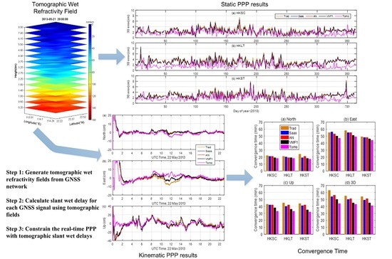
The tropospheric wet delay induced by water vapor is a major error source in precise point positioning (PPP), significantly influencing the convergence time to obtain high-accuracy positioning. Thus, high-quality water vapor information is necessary to support PPP processing. This study presents the use of tomographic wet refractivity (WR) fields in PPP to examine their impacts on the positioning performance. Tests are carried out based on 1-year of 2013 global navigation satellite system (GNSS) observations (30 s sampling rate) from three stations with different altitudes in the Hong Kong GNSS network. Coordinate errors with respect to reference values at a 0.1 m level of convergence is used for the north, east, and up components, whilst an error of 0.2 m is adopted for 3D position convergence. Experimental results demonstrate that, in both static and kinematic modes, the tomography-based PPP approach outperforms empirical tropospheric models in terms of positioning accuracy and convergence time. Compared with the results based on traditional, Saastamoinen, AN (Askne and Nordis), and VMF1 (Vienna Mapping Function 1) models, 23–48% improvements of positioning accuracy, and 5–30% reductions of convergence time are achieved with the application of tomographic WR fields. When using a tomography model, about 35% of the solutions converged within 20 min, whereas only 23%, 25%, 25%, and 30% solutions converged within 20 min for the traditional, Saastamoinen, AN, and VMF1 models, respectively. Our study demonstrates the benefit to real-time PPP processing brought by additional tomographic WR fields as they can significantly improve the PPP solution and reduce the convergence time for the up component.

1. Introduction

The increasingly popular precise point positioning (PPP) technique has been demonstrated to be a potent tool in many Global Navigation Satellite System (GNSS) applications, such as meteorology, precise orbiting, earthquake detection, and precise timing [1,2,3,4]. Atmospheric delays are a major error source in PPP, where the ionospheric delays are often eliminated by combining dual frequency observables [5,6]. For tropospheric delays, they are usually estimated as unknown parameters together with receiver coordinates, receiver clock corrections, and ambiguities [7]. The slant tropospheric delays are, in general, obtained by mapping the zenith tropospheric delay (ZTD) estimated into the signal line-of-sight direction with a mapping function. However, due to the strong correlation between the ZTD and receiver height, it usually requires several tens of minutes to decorrelate these two parameters for convergence, which is a major limitation of PPP in real-time applications [3,8].

With highly accurate tropospheric corrections, it is possible to accelerate the estimation process and improve the PPP results, particularly for the receiver height determination [9]. The tropospheric delay consists of two parts: a hydrostatic component induced by the neutral hydrostatic atmosphere and a wet component caused by the atmospheric water vapor. High-accuracy hydrostatic delay can be determined using empirical zenith hydrostatic delay (ZHD) models combined with mapping functions [10,11]. Though the wet part only accounts for about 10% of the total tropospheric delay, accurately modeling the wet delay is difficult due to its highly dynamic nature in both space and time. Therefore, accurate information of atmospheric water vapor distribution should be very beneficial for PPP processing.

Over the years, many studies have been carried out to provide high-quality tropospheric corrections for PPP. Li et al. proposed to interpolate tropospheric corrections from nearby reference stations to augment PPP for the instantaneous ambiguity-fixing [3]. Hadas et al. evaluated and confirmed the benefits of near real-time tropospheric corrections derived from GNSS processing for PPP [7]. Based on the regional GNSS network, Shi et al. reported a method to augment real-time PPP using a local troposphere model in which the zenith wet delays (ZWDs) of reference stations are fitted by a set of optimal fitting coefficients [12]. Yao et al. investigated the use of ZTDs derived from a GNSS-based global troposphere model as virtual observations to isolate and fix the tropospheric delay in PPP processing [13]. They showed that the proposed algorithm can bring about a 15% improvement in PPP convergence time. With the use of ERA-Interim reanalysis data provided by the European Center for Medium-Range Weather Forecasts (ECMWF), Lou et al. developed an inverse scale height model to generate real-time ZTD grid products based on GPS observations from the Crustal Movement Observation Network of China (CMONOC) [8]. Simulated real-time kinematic GPS-PPP tests showed that the real-time ZTD products can speed up the convergence by up to 29% in the vertical component.

In addition to using the ZTD corrections from a GNSS reference network, many studies have focused on the application of high-quality tropospheric corrections generated by the numerical weather prediction (NWP) in PPP [14,15]. Ibrahim and El-Rabbany examined the effect of NWP-based National Oceanic and Atmospheric Administration Tropospheric Signal Delay Model (NOAATrop) on ionosphere-free PPP solutions [16]. They pointed out that the NOAATrop model accelerated the convergence time by 1%, 10%, and 15% for the latitude, longitude, and height components, respectively, compared to the standard PPP using the Hopfield model. Lu et al. applied the ECMWF derived tropospheric delay parameters in the multi-GNSS PPP processing [17]. The authors presented the improvements of a multi-GNSS PPP solution in both convergence time and positioning accuracy. In a recent study, Wilgan et al. investigated the impact of using tropospheric delays derived from a high-resolution NWP Weather Research and Forecasting (WRF) model in Poland [9]. They demonstrated significant improvements of station coordinates and convergence time by using this strategy in comparison to the PPP approaches where the tropospheric corrections were provided by UNB3m and Forecast Gridded Vienna Mapping Function 1—VMF1-FC. However, a major limitation of using NWP in PPP is data acquisition since the NWP products are difficult to obtain in near-real-time for general users in most regions.

The tomographic technique is a powerful tool for reconstructing the spatiotemporal distribution of atmospheric water vapor with high accuracy [18,19,20,21]. The potential of tomographic water vapor fields in weather forecasting has been demonstrated in various studies [22,23,24,25]. However, the impact of tomographic results on the PPP solution has only received limited attention. In this study, we extend the application of tomographic wet refractivity (WR) fields (a time resolution of 30 min) to constrain tropospheric estimates in real-time PPP processing. The paper is organized as follows. Section 2 describes the study area, data, and methodology used in the study. Section 3 presents the impacts of tomographic WR fields on PPP processing. The evaluation of tomographic SWDs by ECMWF reanalysis data is also described in this section. Finally, the summary is given in Section 4.

2. Methodology

The models employed to obtain ZHD and ZWD corrections, as well as mapping functions, are introduced in this section. In addition, the PPP processing strategy is also described.

2.1. Empirical Tropospheric Models

Assuming the air is an ideal gas and the troposphere satisfies the hydrostatic equilibrium, Saastamoinen et al. developed the following ZHD model that depends on atmospheric pressure [26]:

$$\mathrm{ZHD}=2.2793P_s/\left(1-0.0026\cos 2\phi -0.00028h\right),$$

(1)

where $P_s$ (unit: hPa) is the surface pressure, $\phi$ is the station latitude (unit: radians), and $h$ is the height of the station above sea level (unit: km).

Since atmospheric water vapor is highly variable in both the space and time domains, the ZWD is often difficult to be accurately modeled when only using surface meteorological parameters. Despite this, many ZWD models have been developed in the past decades. As suggested by Reference [11], the Saastamoinen ZWD model is recommended as the optimal model for the China region because of its simplicity and good performance. In addition, when surface meteorological data are unavailable, the best choice is to use the Askne and Nordis (short for AN hereafter) ZWD model with meteorological parameters provided by the GPT2 model. Therefore, both empirical ZWD models will be tested in PPP processing. As for the Saastamoinen model, ZWD is calculated by [27]:

$$\mathrm{ZWD}=0.002277·\left(\frac{1255}{T_s}+0.05\right)·e_s,$$

(2)

where $T_s$ (unit: Kelvin degrees) and $e_s$ (unit: hPa) represent the surface temperature and water vapor pressure, respectively. The AN ZWD model reads as follows [28]:

$$\mathrm{ZWD}={10}^{-6}·\left(22.972+375463/T_m\right)·\frac{287.053}{\left(\omega +1\right)·g_m}·e_s,$$

(3)

where $T_m$ and $\omega$ are the weighted mean temperature and water vapor decrease factor, respectively, which can be provided by the GPT2w model [10]. $g_m$ is the gravity acceleration that can be calculated from empirical model with latitude and height. In addition, the Vienna mapping functions 1 (VMF1) can provide ZHD and ZWD values on global grids that have been determined from forecasting data of the ECMWF. The 24-h forecasting products (ZHD, ZWD and VMF1 coefficients) have a good performance and, thus, are also examined in our real-time PPP analysis [29]. In the PPP processing, the slant tropospheric delays are calculated by mapping the zenith delays into the radio line-of-sight direction with the VMF1 since it is the most accurate mapping function for the entire history of space geodetic observations [29,30].

2.2. Tropospheric Delay Derived from Tomographic WR Field

Tropospheric wet delays can be accurately calculated if the full humidity profile is known. The tomographic technique is a powerful tool for modeling atmospheric water vapor with high spatiotemporal resolutions [18,31]. A multi-source water vapor tomography system has been developed in Hong Kong as reported by Reference [21]. The tomographic products have been successfully used for detecting the water vapor variability during heavy precipitation events in Hong Kong [25]. In the present work, we further apply the tomographic WR fields in PPP processing. The slant wet delays (SWDs) used for reconstructing the WR field were derived from the double difference observations as processed by the Bernese 5.2 software. The zero difference residuals are extracted from the double difference residuals by using the method proposed by Alber et al. [32]. In the tomography, both horizontal constraints and vertical a priori information averaged from 3-day radiosonde measurements were adopted to solve the WR fields. With the use of tomographic WR fields, the SWD along the ray path from a receiver to a satellite can be yielded as

$$\mathrm{SWD}={{\displaystyle \sum }}_{i=1}^n{N}_{wi}{d}_i,$$

(4)

where $n$ is the number of tomographic voxels crossed by the SWD, $N_{wi}$ is the WR in the voxel $i$, and $d_i$ is the length of the ray path within the voxel $i$. In this study, the tomographic discretization model determined in Reference [33] is employed.

2.3. PPP Processing Strategy

The ionosphere-free carrier phase observation used in PPP can be expressed as

$$l=\mathit{u}\ast {\mathit{\delta }}_r+{\delta }_c+a+{\delta }_T+ϵ,$$

(5)

$${\delta }_T=m_{\mathrm{zwd}}\ast \mathrm{ZWD}+m_{gN}\ast g^N+m_{gE}\ast g^E$$

$$m_{gN}=\frac{\cos \left(azi\right)}{\sin \left(ele\right)\tan \left(ele\right)+0.003},m_{gE}=\frac{\sin \left(azi\right)}{\sin \left(ele\right)\tan \left(ele\right)+0.003}$$

where $l$ represents the misclosure value in length units; $\mathit{u}$ is the unit vector of the direction from the receiver to the satellite observed (with elevation angle $ele$ and azimuth angle $azi$); ${\mathit{\delta }}_r$ is the correction to the approximate receiver position; ${\delta }_c$ stands for receiver clock error in meters; $a$ denotes the float ambiguities scaled to meters, which are also designed to partially absorb residual systematic errors, hence, no attempt is made to fix it; ${\delta }_T$ represents the residual slant tropospheric delays, it is associated with the zenith wet delay ($\mathrm{ZWD}$) and horizontal gradient delays ($g^N$ and $g^E$) through corresponding mapping functions $m_{\mathrm{zwd}}$ and ($m_{gN}$ and $m_{gE}$), respectively; $ϵ$ is the observation error, assumed to be normal distributed and the variance is calculated based on the elevation-dependent weighting model. Corrections projected to the line of sight are applied for satellite clock error, hydrostatic delay, tidal loadings, relativistic effects, earth rotation, antenna phase center corrections, and wind-up effects [34]. The Kalman filter is applied to estimate the parameters [5]. The zenith wet delay is estimated as a 1-h constant and the gradients are parameterized as 1-day constants.

In traditional PPP, the convergence of the position highly depends on the accurate estimation of tropospheric delays [13] and, in general, requires a sufficiently long observation time span (for example, dozens of minutes) to reach the cm level. This process can be shortened by incorporating external troposphere information. In our study, estimation augmentations for tropospheric parameters are implemented via applying the following constraints

$$\mathrm{ZWD}-{\mathrm{ZWD}}_{model}~\mathrm{N}\left(0,{\sigma }_{\mathrm{zwd},model}^2\right)$$

For the tomography model which provides slant delays, both the $\mathrm{ZWD}$ and gradient parameters are constrained in

$${\delta }_T-{\delta }_{T\_model}~\mathrm{N}\left(0,{\sigma }_{T\_model}^2\right),{\sigma }_{T\_model}^2\approx m_{\mathrm{zwd}}^2\ast {\sigma }_{\mathrm{zwd}\_model}^2$$

where ${\sigma }_{\mathrm{zwd}\_model}$ represents the standard deviation of the ZWD provided by the apriori model. Its values are set as 38 mm, 35 mm, 10 mm, and 7 mm for the Saastamoinen, AN, VMF1, and tomography models, respectively, which were derived from our model evaluation results.

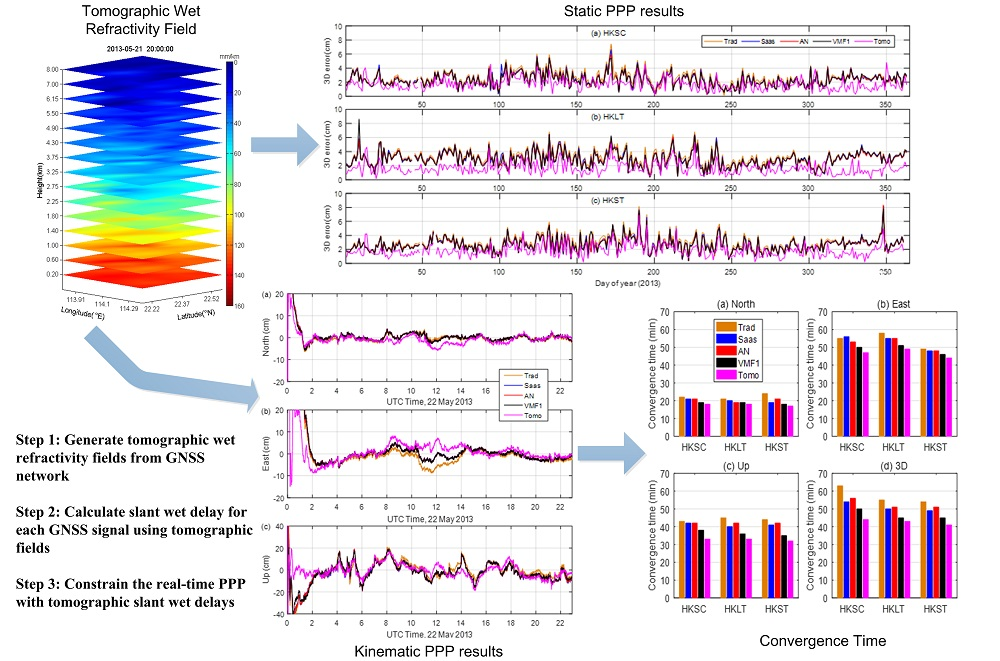
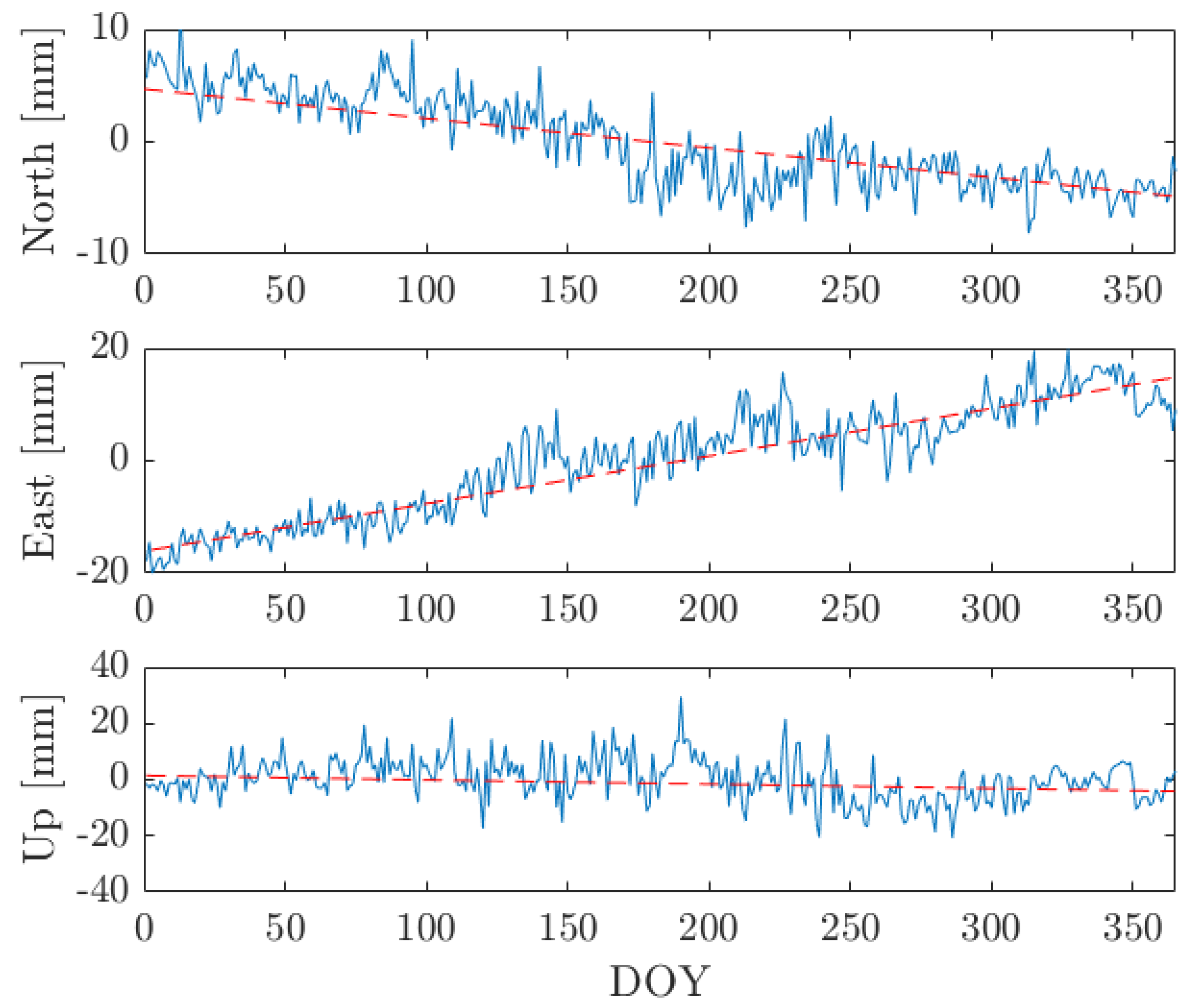
To understand the positioning performance, PPP results are derived using Bernese 5.2 software [35] and then linearly fitted as the reference solution (see

Table 1. The reference coordinates based on Bernese PPP (precise point positioning).

Station	North (m)	East (m)	Up (m)
HKLT	2,483,181.3881 + (−0.0280 × DOY + 5.1185) × 10−3	808,564.3867 + (0.0826 × DOY − 15.1100) × 10−3	125.8913 + (−0.0120 × DOY + 2.1869) × 10−3
HKSC	2,469,482.0314 + (−0.0353 × DOY + 6.4634) × 10−3	514,546.6899 + (0.0894 × DOY − 16.3550) × 10−3	20.2015 + (−0.0228 × DOY + 4.1775) × 10−3
HKST	2,477,581.4294 + (−0.0324 × DOY + 5.9206) × 10−3	518,972.5105 + (0.0850 × DOY − 15.5520) × 10−3	258.6856 + (−0.0200 × DOY + 3.6576) × 10−3

and Figure 1). We use self-developed software for PPP data processing, which can be easily adapted to include the various tropospheric correction models. IERS conventions required for PPP are included in the software to ensure the consistency with Bernese.

3. Experiments and Results

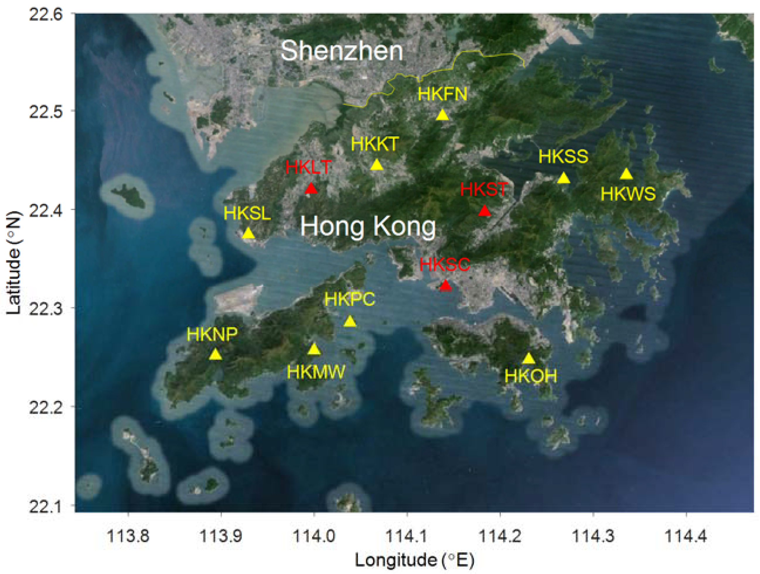
The Lands Department of the Government of Hong Kong Special Administrative Region (HKSAR) has been operating the Hong Kong GNSS network since 2000 [36]. Before 2015, this network consisted of 12 GNSS stations, and their locations are shown in Figure 2. At present, the GNSS network contains 18 stations and the number is still in increase. We processed the data (interval is 30 s) from three GNSS stations of the Hong Kong network over the whole year of 2013. The three stations have relatively large differences in their heights: HKSC (at height of 20 m), HKLT (at height of 126 m), and HKST (at height of 259 m). The top boundary of the tomographic model is set to 8.5 km, as the atmosphere above this height in Hong Kong can be regarded as dry air. In the vertical direction, the troposphere is discretized into 15 nonuniform layers. From the ground to the top, the layer thickness is arranged as follows: 400 m for the bottom five layers, 500 m for the next four layers, 600 m for the next three layers, 700 m for one layer, and 1000 m for the top two layers. In the horizontal direction, resolutions of 0.08° (about 8.5 km) are determined for both latitude and longitude directions. In the tests for the HKSC station, only 11 stations except for HKSC were adopted in reconstructing the WR fields, and same for HKLT and HKST stations. This makes sure that the tomographic WR fields are independent on the testing stations. Based on this tomographic model, SWDs derived from the tomographic WR fields using multi-source data in Hong Kong have an accuracy of better than 12 mm [21]. The WR fields generated by the tomography have a temporal resolution of 30 min. To examine their applicability in real-time PPP, tomographic WR fields generated for the last 30 min are adopted for the current processing.

Observations with elevation angles below 5° are not used. The five tropospheric delay correction schemes, that is, the traditional (ZWD is estimated without priori model constraints), Saastamoinen, AN, VMF1, and tomographic WR fields, are tested in the PPP in both static and kinematic modes. Position errors relative to the ground truth values are used as the indicators for understanding the convergence performance of the positioning. The threshold of convergence (sequential 10 epochs are checked) is set to 0.1 m for each coordinate component, and 0.2 m for the three-dimensional (3D) position, a similar configuration can be found in Reference [37].

3.1. Evaluation of Tomographic SWDs by ECMWF

Prior to the application of tomographic SWDs in PPP processing, we evaluated their quality by ECMWF ERA-Interim reanalysis products. ERA-Interim covers the period from 1 January 1979 onwards and continuously extends forward in near-real time [38]. In the generation of reanalysis products, various observations including synoptic stations, ships, ocean-buoys, radiosonde stations, aircraft, and remote sensing observations were adopted to recreate the past atmospheric conditions [38]. Reanalysis data provide a good quality of global atmospheric profiles, thus, they have been widely used in research such as data evaluation, meteorology, and climate change. ERA-Interim reanalysis products have a 6 h time resolution and 10 different horizontal resolutions varying from 0.125° × 0.125° to 3° × 3°. Our comparison adopted the reanalysis products with the highest resolution of 0.125° × 0.125° since Hong Kong is a small region. We calculated the SWDs of all the 12 GNSS stations from both tomographic WR fields and ERA-Interim reanalysis products over the whole month of May 2013 for a direct comparison.

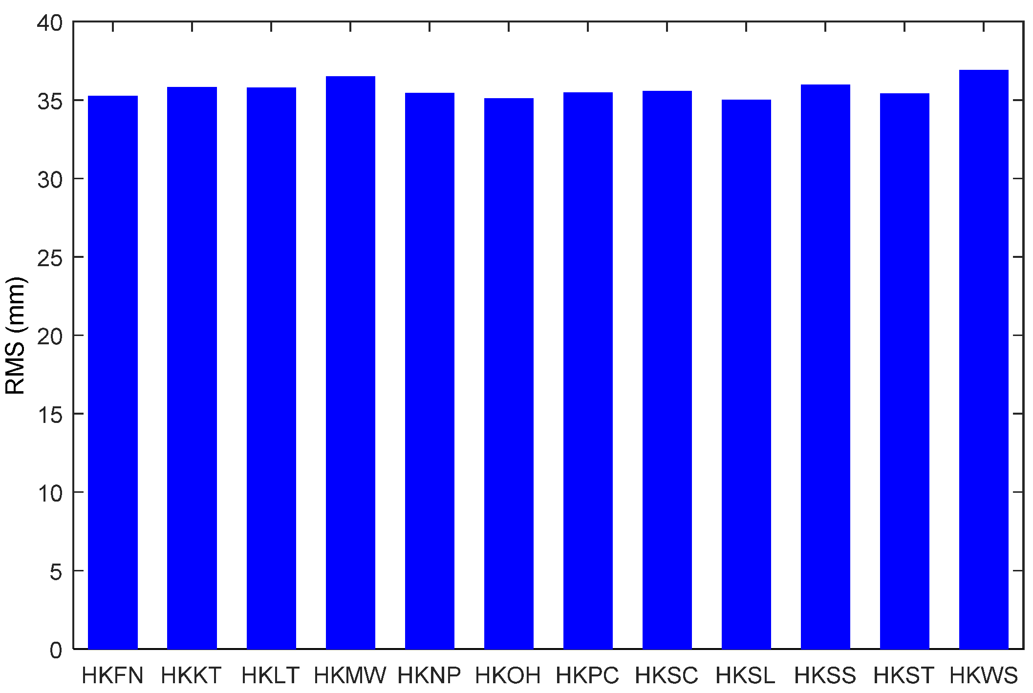
In

Table 2. The comparisons of SWDs (tomography minus ECMWF) derived from tomographic WR fields and ERA-Interim reanalysis for 12 GPS sites for the period 1–31 May 2013.

Comparison	Elevation
	5–10°	10–15°	15–20°	20–30°	30–60°	>60°	5–90°
Bias (mm)	16.24	4.62	2.57	0.78	−2.66	−3.24	0.57
RMS (mm)	91.36	45.62	38.67	33.63	21.24	14.78	35.65

, the comparison (tomography minus ECMWF) between tomography and ECMWF for all SWDs with elevation angles ranging from 5° to 90° yielded a bias of −0.57 mm and an RMS error of 35.65 mm. Table 2 also gives the statistics of the SWD comparison at different elevation intervals. We can observe that RMS error decreases quickly as elevation increases. RMS error for SWDs of elevations between 5° and 10° is more than 6 times the RMS error of SWDs with elevations greater than 60°. Tomographic SWDs between 5–10° achieved an RMS error of 91.36 mm when compared with ECMWF. For elevations higher than 60°, the RMS error reduces to 14.78 cm. The quality of tomographic SWDs degrades with the elevation decreasing is likely to be explained by (1) a GNSS signal at a lower elevation taking a long time to propagate through the troposphere and, thus, has a larger wet delay; and (2) GNSS measurements at low elevations are susceptible to the multipath effect that can greatly degrade the quality of inferred SWDs and, thus, result in less accurate tomographic solutions. Figure 3 further exhibits RMS errors for SWDs above 5° at the 12 GNSS stations. The RMS errors of tomographic SWDs vary in the range of 35–37 mm when compared with ECMWF data. In general, the comparison demonstrates that tomographic WR fields can provide SWDs with cm-level accuracy for PPP processing.

3.2. Static PPP Solutions

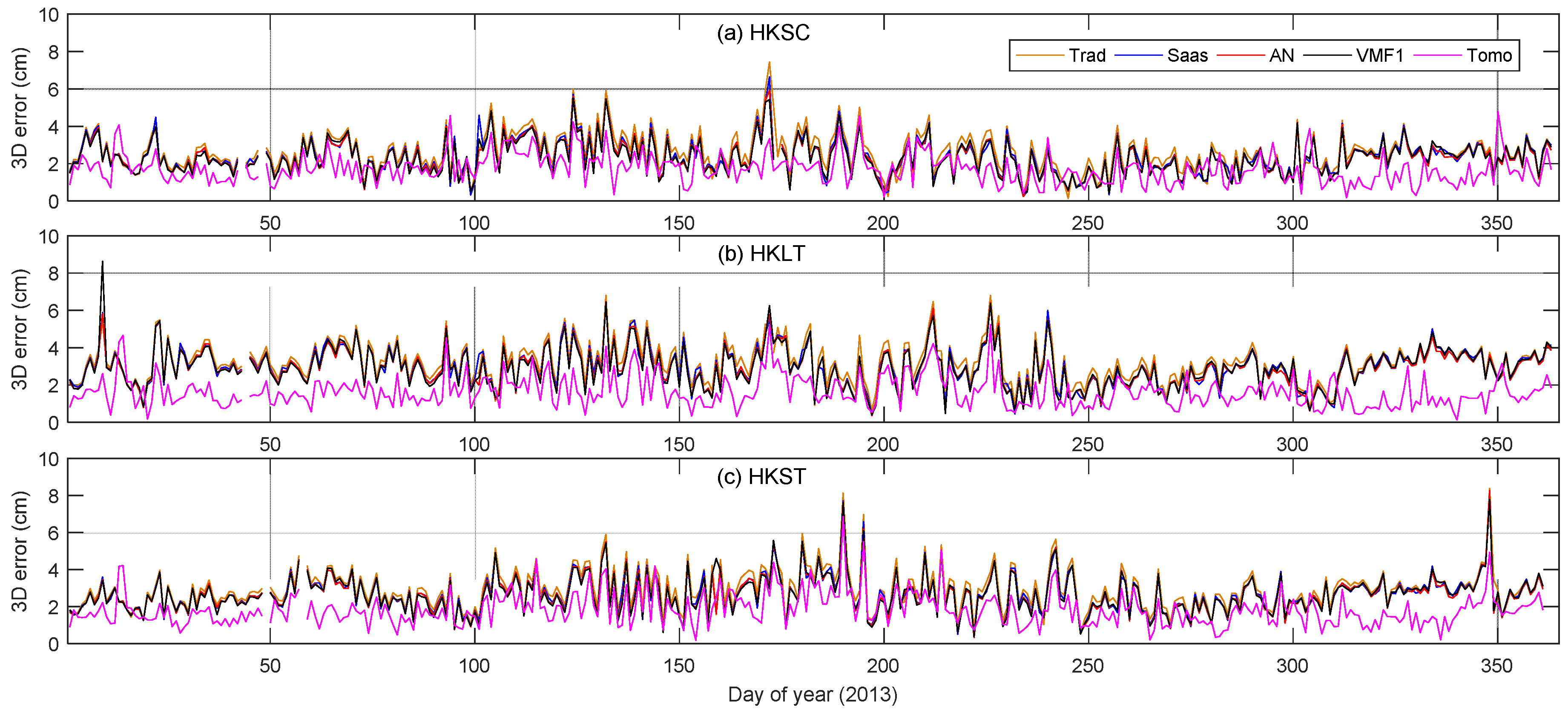
Figure 4 presents the time series of 3D errors (relative to the ground truth values) obtained for the three stations over the whole year of 2013. Figure 4 shows that, for all the three stations, the 3D errors for the tomography model are in general smaller than those based on the traditional, Saastamoinen, AN, and VMF1 models. The tomography generally shows a consistently better performance throughout the year. Due to the severer water vapor variations, the rainy season (DOY 120~250) has a larger fluctuation in 3D error than other days. The traditional, Saastamoinen, AN, and VMF1 models exhibit comparable performance with 3D errors up to 9 cm. Using the tomography model, the 3D errors are less than 3 cm in general (mostly less than 2 cm).

Table 3. The statistical results (model minus reference) for the PPP static positioning using the traditional (Trad), Saastamoinen (Saas), Askne and Nordis (AN), VMF1, and tomography (Tomo) models. The biases and RMS errors in the north, east, and up directions, as well as 3D RMS, were calculated from the observations over the whole of 2013.

Stations	Models	North (cm)		East (cm)		Up (cm)		3D RMS (cm)
		Bias	RMS	Bias	RMS	Bias	RMS
HKSC	Trad	0.12	0.39	−0.45	0.91	2.30	2.58	2.76
	Saas	0.14	0.40	−0.46	0.92	1.99	2.31	2.52
	AN	0.14	0.40	−0.47	0.92	1.94	2.26	2.47
	VMF1	0.14	0.40	−0.47	0.92	1.93	2.24	2.46
	Tomo	−0.38	0.59	−0.53	1.05	0.04	1.22	1.72
HKLT	Trad	−0.42	0.58	−0.16	0.74	3.00	3.19	3.33
	Saas	−0.43	0.58	−0.14	0.75	2.73	2.96	3.11
	AN	−0.43	0.58	−0.14	0.75	2.67	2.90	3.06
	VMF1	−0.43	0.58	−0.15	0.78	2.66	2.90	3.06
	Tomo	−0.19	0.48	−0.39	0.93	0.06	1.36	1.73
HKST	Trad	−0.35	0.52	−0.45	0.88	2.62	2.85	3.03
	Saas	−0.34	0.51	−0.47	0.90	2.34	2.59	2.79
	AN	−0.34	0.51	−0.47	0.90	2.31	2.56	2.76
	VMF1	−0.34	0.51	−0.48	0.90	2.30	2.56	2.76
	Tomo	−0.29	0.53	−0.48	0.96	0.46	1.26	1.67

presents the mean biases and root mean square (RMS) errors in the north, east, and up components as well as the 3D RMS values for all stations averaged from the whole year of 2013, in order to further assess the impact of using the particular models. It can be seen that the biases and RMS errors in the north and east components of each station are comparable for traditional, Saastamoinen, AN, and VMF1 models. No obvious improvements in the north and east components can be observed from the static PPP results using tomography. However, significant differences in the statistics exist for the up component. The mean biases of the up component, calculated by the means of the tomography model are significantly smaller than those calculated with the Saastamoinen, AN, VMF1, and traditional models. In addition, the up component errors vary in the range 2.2–3.2 cm for the traditional, Saastamoinen, AN, and VMF1 models, while smaller than 1.4 cm for the tomography model. The up RMSs are directly reflected in the 3D RMSs where, again, the application of tomography derived wet delays results in the smallest 3D RMS errors, with the best value of 1.67 cm for HKST station. In general, the tomographic products can reduce the 3D RMS error by 0.7–1.6 cm compared with the other four models. We can also observe that the traditional model yields the largest 3D RMS at all the three stations, indicating that the use of a priori ZWD information in PPP processing would further improve the results.

3.3. Kinematic PPP Solutions

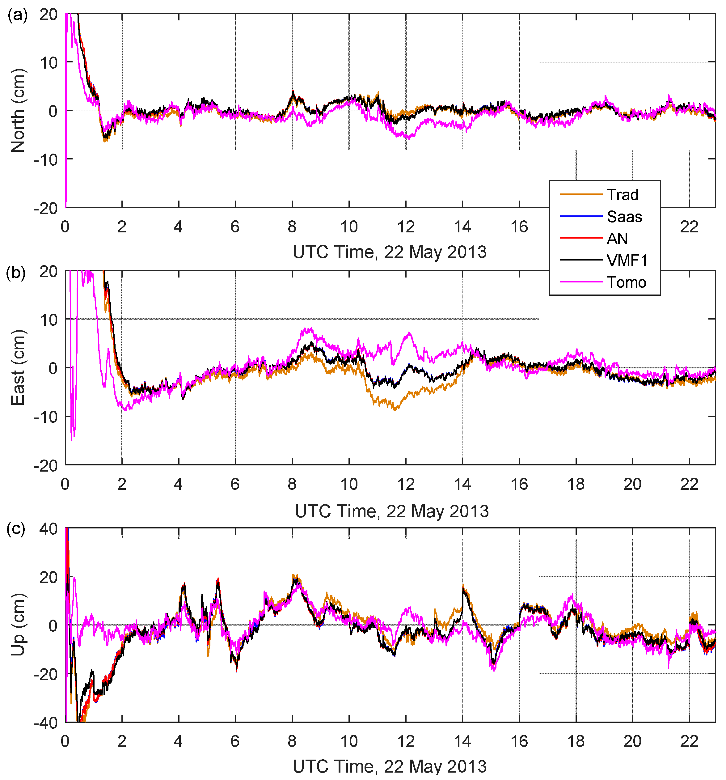
As mentioned before, the tropospheric delay is highly correlated with the height, thus, the kinematic PPP is expected to benefit a lot from using tomographic WR fields. We further investigated the performance of kinematic processing results over time using the different tropospheric correction methods. Note that the tested GNSS data have a 30-s sampling rate. With the assumption that the PPP solutions require 2 h to converge, we excluded the first 2 h of the results in our analysis. Figure 5 shows the time series of kinematic coordinate errors at sample station HKLT on 22 May 2013. It is shown that the filter is initialized at the beginning of the processing and takes about 2 h to converge.

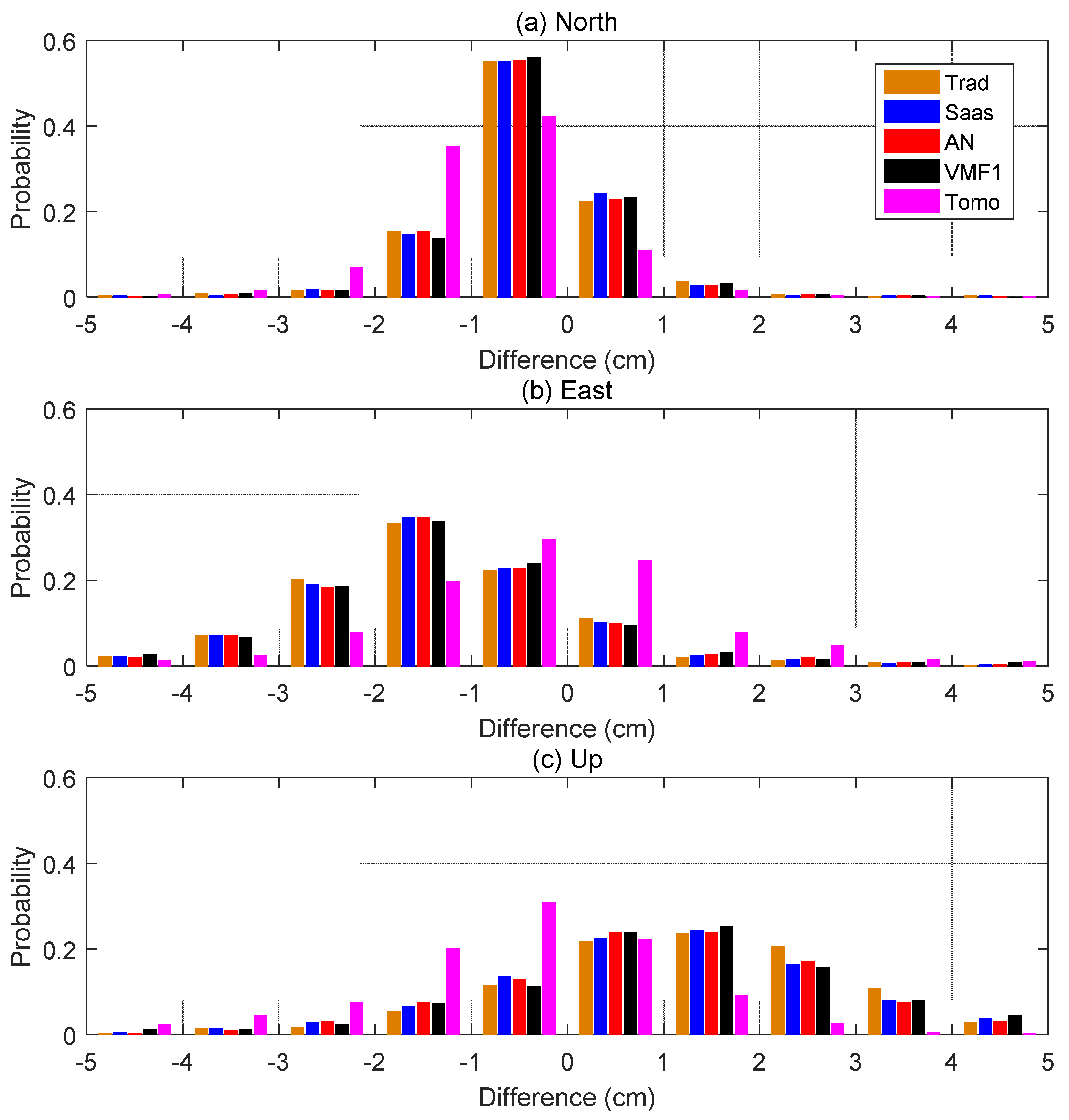
The histograms of the coordinate errors from all stations over the whole year period for the five models are shown in Figure 6. The distributions of coordinate errors of the three components for the traditional, Saastamoinen, AN, and VMF1 models look similar. However, the coordinate error distributions for the tomography vary greatly with the other four models. In the north component, the tomography shows a more prominent negative bias than the other four models. For the east and up components, the tomography-based approach exhibits position errors distributed much closer to the corresponding centers, although the biases therein are also viewable. There is a higher probability of a large negative/positive position error for traditional, Saastamoinen, AN, and VMF1 models than the tomography in the east/up component.

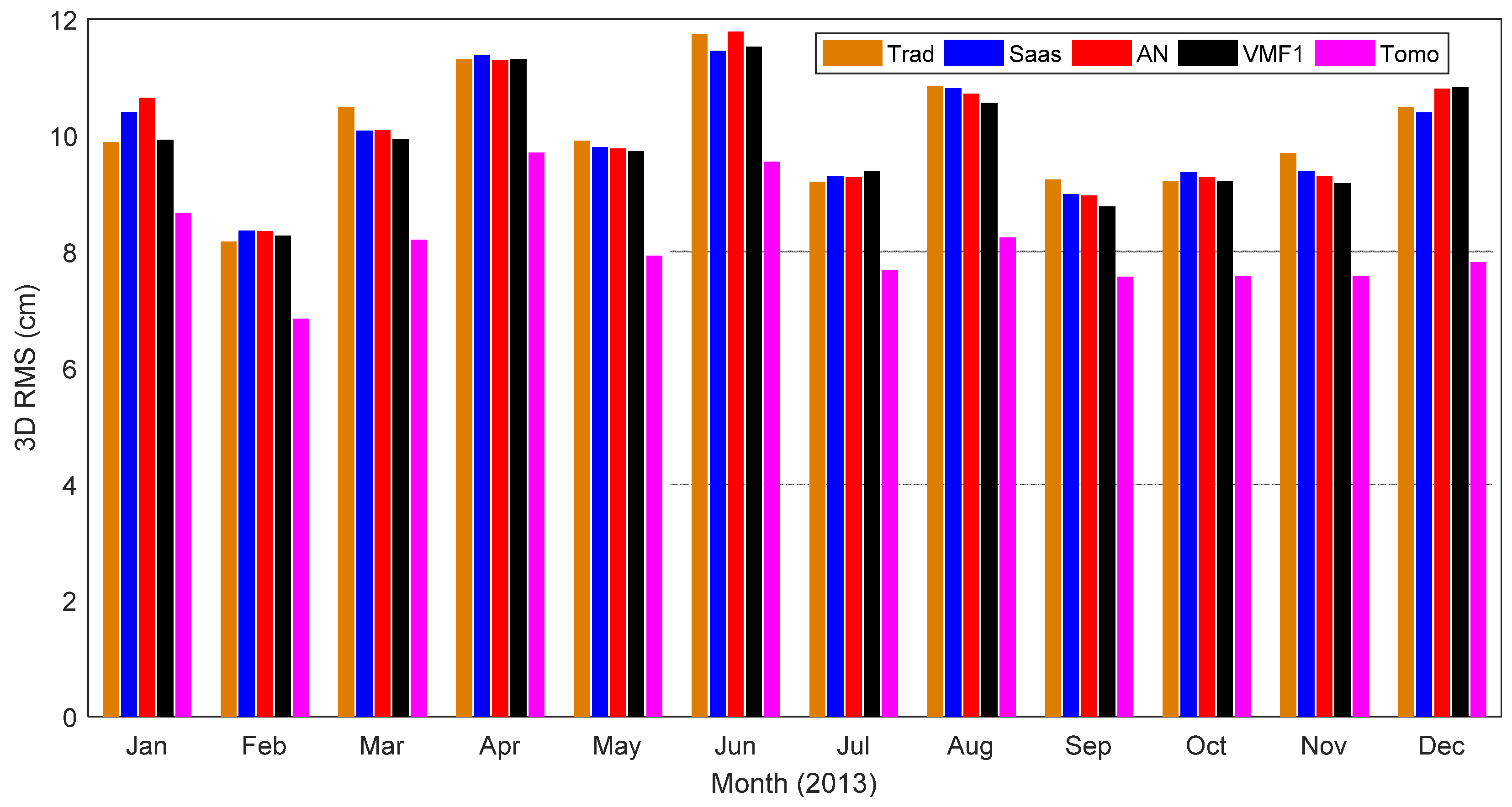
Figure 7 exhibits the 3D RMSs derived from the kinematic PPP results of all the stations for the 12 months in 2013. Tomography based results achieve the best performance in all 12 months, with 3D RMSs varying in the range of 6–10 cm.

Table 4. The statistical results (model minus reference) for the PPP kinematic positioning using the traditional (Trad), Saastamoinen (Saas), Askne and Nordis (AN), VMF1, and tomography (Tomo) models. The biases and RMS errors in the north, east, and up directions, as well as 3D RMS, were calculated from the observations over the whole year of 2013.

Stations	Models	North (cm)		East (cm)		Up (cm)		3D RMS (cm)
		Bias	RMS	Bias	RMS	Bias	RMS
HKSC	Trad	−0.24	2.88	−0.88	4.42	0.87	9.22	10.63
	Saas	−0.23	2.96	−0.87	4.51	0.54	9.35	10.80
	AN	−0.21	2.91	−0.93	4.48	0.54	9.12	10.57
	VMF1	−0.21	2.87	−0.96	4.52	0.63	9.35	10.77
	Tomo	−1.19	2.98	−0.05	4.02	−0.64	6.39	8.11
HKLT	Trad	−0.33	2.52	−1.43	4.53	2.07	8.76	10.18
	Saas	−0.35	2.44	−1.53	4.29	1.81	8.72	10.02
	AN	−0.35	2.45	−1.43	4.42	1.76	7.49	9.88
	VMF1	−0.35	2.49	−1.37	4.40	1.79	8.56	9.95
	Tomo	−0.66	2.47	−0.33	3.86	−0.80	5.76	7.36
HKST	Trad	−0.54	2.54	−1.46	4.23	1.47	8.74	10.04
	Saas	−0.54	2.49	−1.47	4.33	1.23	8.79	10.11
	AN	−0.52	2.45	−1.48	4.27	1.16	8.57	9.89
	VMF1	−0.52	2.39	−1.52	4.17	1.26	8.48	9.75
	Tomo	−0.82	2.46	−0.50	3.62	−0.33	6.10	7.51

further gives the mean biases and RMSs from all stations and models for the north, east and up components. As shown in Table 4, similarly to the static PPP case, kinematic solutions using a tomography model have the smallest 3D RMS errors. The smallest 3D RMS is achieved at the HKLT station with a value of 7.36 cm. For the traditional, Saastamoinen, AN, and VMF1 models, the 3D RMS errors of the HKLT station are 10.18 cm, 10.02 cm, 9.88 cm, and 9.95 cm, respectively. As observed from all stations, the tomography model can achieve 2–3 cm 3D RMS reduction. In Table 4, we can also observe that the 3D RMS statistics is mainly affected by the up component. The traditional, Saastamoinen, AN, and VMF1 models have up biases and RMS errors varying in the range of 0.5–2.1 cm and 7.4–9.4 cm, respectively. Much smaller up RMS errors as low as −5.76 cm are observed for the tomography model, hence, the tomographic solutions can significantly improve the performance of a kinematic PPP. In addition, compared with the other four models, the tomography model slightly improves the kinematic PPP solutions in the east component. However, for the north component, the kinematic PPP solutions obtained with the tomography model are at a similar level with those processed by the traditional, Saastamoinen, AN, and VMF1 models. Thus, one may conclude that the accurate tropospheric delay corrections have the biggest benefit to the up component estimation for the PPP processing.

3.4. Convergence Time

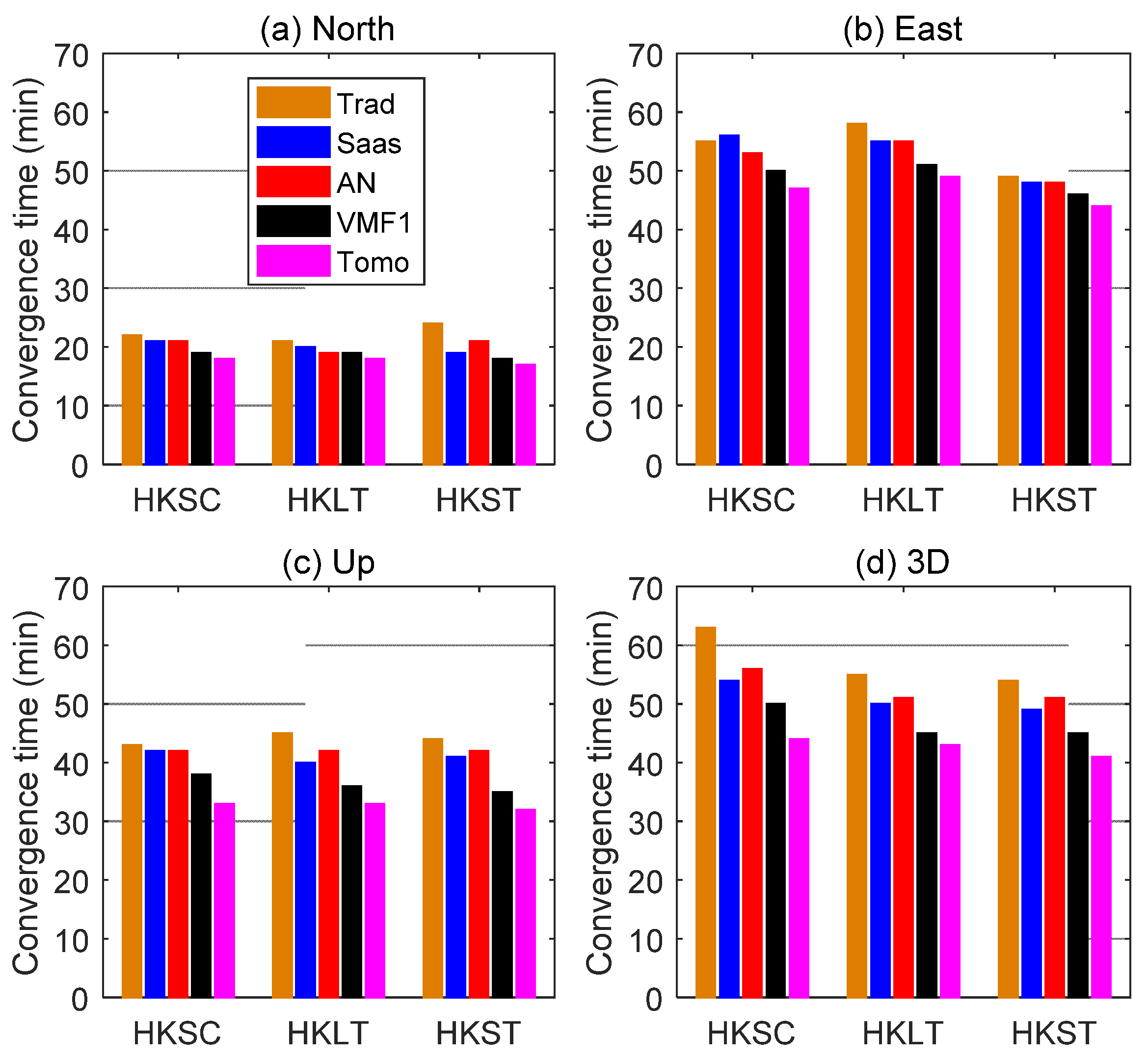
Based on the kinematic PPP results for the whole year of 2013, we further analyzed the time required for position converge. For the three coordinate components, when the corresponding errors with respect to reference values remain below 0.1 m for at least 10 epochs afterward, they are considered converged, whilst the error of 0.2 m is adopted for 3D position convergence. Figure 8 shows the convergence times for three Hong Kong stations and five tropospheric correction methods averaged over the whole year of 2013. The tomography-based solutions have a shorter convergence time compared to the traditional, Saastamoinen, AN, and VMF1 models, which is especially obvious in the up component. This finally results in a higher convergence performance in the 3D position when the tomographic method is applied.

Table 5. The means and standard deviation (STDs) of convergence times for the five methods averaged from the whole year of 2013 for each station.

Stations	Models	North (min)		East (min)		Up (min)		3D (min)
		Mean	STD	Mean	STD	Mean	STD	Mean	STD
HKSC	Trad	22	22	55	45	43	29	63	71
	Saas	21	21	56	50	42	29	54	42
	AN	21	22	53	43	42	30	56	51
	VMF1	19	23	50	40	38	41	50	45
	Tomo	18	17	47	38	33	33	44	35
HKLT	Trad	21	17	58	44	45	34	55	35
	Saas	20	15	55	41	40	31	50	32
	AN	19	14	55	42	42	32	51	33
	VMF1	19	14	51	39	36	29	45	31
	Tomo	18	14	49	37	33	24	43	27
HKST	Trad	24	19	49	32	44	32	54	32
	Saas	19	13	48	32	41	30	49	29
	AN	21	15	48	32	42	30	51	31
	VMF1	18	12	46	32	35	26	45	27
	Tomo	17	11	44	30	32	22	41	23

gives the means and standard deviations (STDs) of convergence times averaged over the whole year of 2013 for the three stations. For the north and east components, the tomography yields a slightly smaller convergence time compared with the other four models. However, in the up component, the tomography method takes about 32 min to convergence below 0.1 m, whereas the convergence times are about 44 min, 41 min, 42 min, and 36 min for the traditional, Saastamoinen, AN, and VMF1 methods, respectively. In terms of the 3D position, the tomography approach reduces the convergence time by 4–30% compared to the other four models.

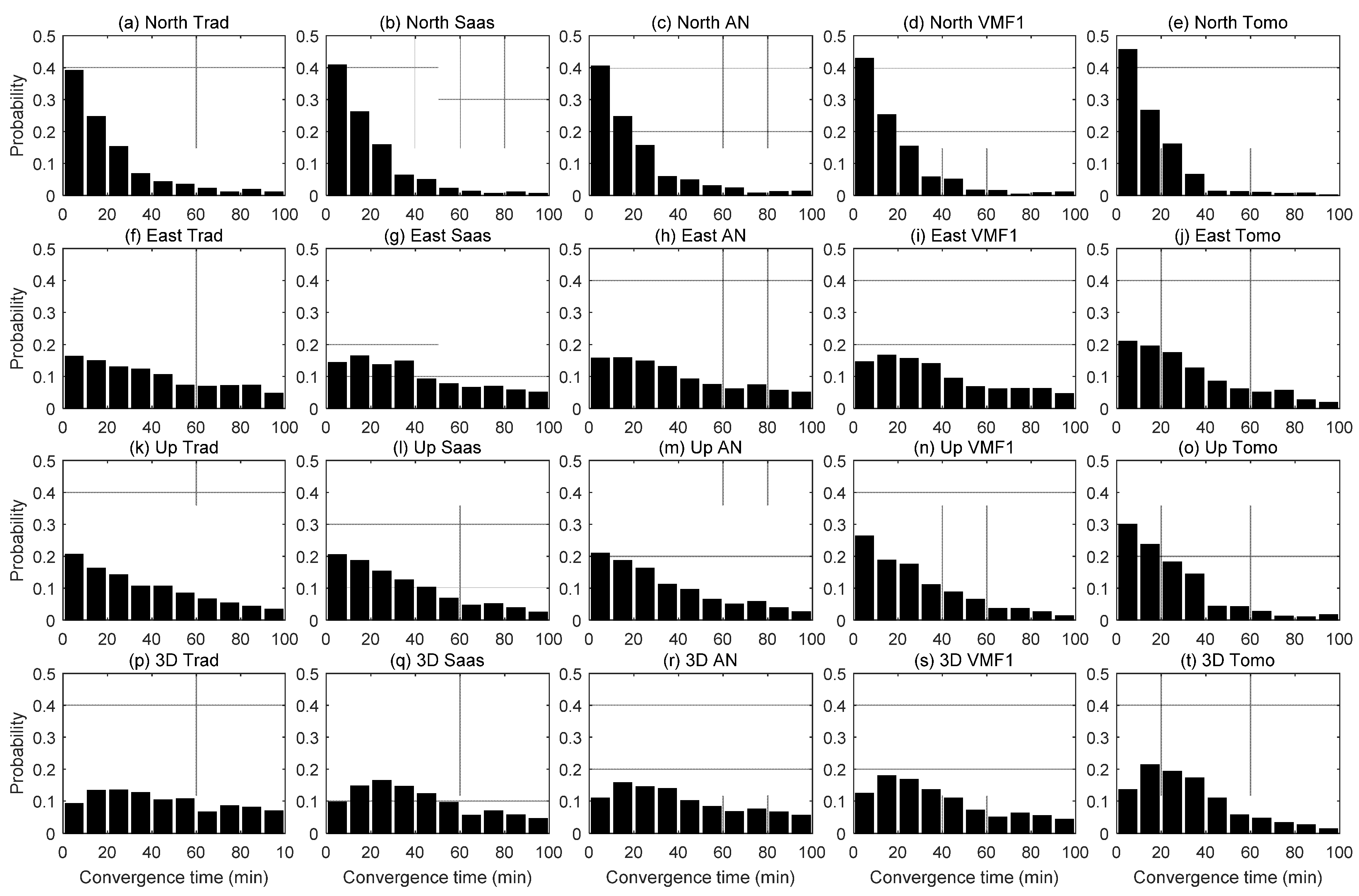
Finally, we examined the histograms (see Figure 9) of the convergence times for the north, east, and up components and the 3D position. Within 20 min, 73% of the solutions by tomography converged for the north component, while for the other four models 64–68% solutions converged. In the east component, 40% tomography-based solutions converged within 20 min while ~31% converged for the other models. For the up component, about 54% of the solutions converged within 20 min for the tomography model, whereas only 36%, 39%, 39%, and 45% solutions converged within 20 min for the traditional, Saastamoinen, AN, and VMF1 models. For the 3D position, 23%, 24%, 25%, 30%, and 35% of solutions converged within 20 min for the traditional, Saastamoinen, AN, VMF1, and tomography models, respectively. Thus, using the tomography model is especially useful for shortening the convergence time on up component.

4. Conclusions

Since the tropospheric effects are frequency independent for the GNSS signals, the tropospheric ZWDs, in general, are estimated as additional parameters in the traditional PPP data processing. With additional accurate wet delay information, it is possible to reduce the positioning convergence time and improve the PPP results. We have analyzed the impact of tomographic WR fields on the determination of positioning components and convergence time in both static and kinematic PPP.

Three GNSS stations with relatively large height differences from the Hong Kong GNSS network were employed in this paper. Performance tests were conducted using GNSS observations collected at these sites over the whole year of 2013. For a direct comparison, we also examined the impacts of using traditional, Saastamoinen, AN (Askne and Nordis), and VMF1 models on the PPP estimation process. In the data analysis, PPP positioning resulting from both static and kinematic modes were presented and discussed.

For the static PPP processing, the 3D RMS errors obtained by applying the tomography model were less than 3 cm in general, which were about 1 cm smaller than those for the traditional, Saastamoinen, AN, and VMF1 models. The statistics in the north and east components are similar for all five tropospheric correction models. However, for the up component, the tomography-based solutions offer a significantly better performance than those of the other four models. The tomographic products can reduce the 3D RMS error of the static PPP by about 0.7–1.6 cm.

For the kinematic PPP processing, the traditional, Saastamoinen, AN, VMF1, and tomography models exhibited comparable statistics for the north and east components, while the tomography-based solutions were much better in the up component. Consequently, the 3D RMS errors for the tomography-based solutions were about 2 cm smaller than for those based on the other four models. The 3D statistics for the kinematic PPP processing directly reflects the up component behavior. Thus, we can conclude that the tomographic delay corrections benefit the up component estimation most for the kinematic PPP processing.

In addition, we investigated the convergence time for all tropospheric correction models using kinematic PPP results. In terms of the 3D position, the convergence times for tomography are 14–30%, 14–19%, 16–20%, and 5–12% shorter than for the traditional, Saastamoinen, AN, and VMF1 models, respectively. About 35% of the solutions converged within 20 min for tomography model, whereas only 23%, 24%, 25%, and 30% solutions obtained convergences within 20 min for the traditional, Saastamoinen, AN, and VMF1 models. Thus, using the tomographic SWDs is also beneficial for shortening the convergence time on kinematic PPP processing. This study demonstrated the significant improvement in PPP processing with the use of high-quality tomographic WR fields instead of empirical tropospheric models. Consequently, except for applications in meteorology, it is expected that the tomographic products will also benefit a lot to the real-time PPP processing.

References

- Zumberge, J.F.; Heflin, M.B.; Jefferson, D.C.; Watkins, M.M.; Webb, F.H. Precise point positioning for the efficient and robust analysis of GPS data from large networks. J. Geophys. Res. Solid Earth 1997, 102, 5005–5017. [Google Scholar] [CrossRef] [Green Version]
- Kouba, J. A possible detection of the 26 December 2004 Great Sumatra-Andaman Islands Earthquake with solution products of the International GNSS Service. Stud. Geophys. Geod. 2005, 49, 463–483. [Google Scholar] [CrossRef]
- Li, X.; Zhang, X.; Ge, M. Regional reference network augmented precise point positioning for instantaneous ambiguity resolution. J. Geodesy 2011, 85, 151–158. [Google Scholar] [CrossRef]
- Yuan, Y.; Zhang, K.; Rohm, W.; Choy, S.; Norman, R.; Wang, C.-S. Real-time retrieval of precipitable water vapor from GPS precise point positioning. J. Geophys. Res. Atmos. 2014, 119, 10044–10057. [Google Scholar] [CrossRef] [Green Version]
- Leick, A.; Rapoport, L.; Tatarnikov, D. GPS Satellite Surveying, 4th ed.; Wiley: Hoboken, NJ, USA, 2015; ISBN 978-1-118-67557-1. [Google Scholar]
- Luo, X.; Lou, Y.; Xiao, Q.; Gu, S.; Chen, B.; Liu, Z. Investigation of ionospheric scintillation effects on BDS precise point positioning at low-latitude regions. GPS Solut. 2018, 22. [Google Scholar] [CrossRef]
- Hadas, T.; Kaplon, J.; Bosy, J.; Sierny, J.; Wilgan, K. Near-real-time regional troposphere models for the GNSS precise point positioning technique. Meas. Sci. Technol. 2013, 24, 055003. [Google Scholar] [CrossRef]
- Lou, Y.; Huang, J.; Zhang, W.; Liang, H.; Zheng, F.; Liu, J. A New Zenith Tropospheric Delay Grid Product for Real-Time PPP Applications over China. Sensors 2017, 18, 65. [Google Scholar] [CrossRef] [PubMed]
- Wilgan, K.; Hadas, T.; Hordyniec, P.; Bosy, J. Real-time precise point positioning augmented with high-resolution numerical weather prediction model. GPS Solut. 2017. [Google Scholar] [CrossRef]
- Böhm, J.; Möller, G.; Schindelegger, M.; Pain, G.; Weber, R. Development of an improved empirical model for slant delays in the troposphere (GPT2w). GPS Solut. 2015, 19, 433–441. [Google Scholar] [CrossRef]
- Chen, B.; Liu, Z. A Comprehensive Evaluation and Analysis of the Performance of Multiple Tropospheric Models in China Region. IEEE Trans. Geosci. Remote Sens. 2016, 54, 663–678. [Google Scholar] [CrossRef]
- Shi, J.; Xu, C.; Guo, J.; Gao, Y. Local troposphere augmentation for real-time precise point positioning. Earth Planets Space 2014, 66, 30. [Google Scholar] [CrossRef] [Green Version]
- Yao, Y.; Yu, C.; Hu, Y. A New Method to Accelerate PPP Convergence Time by using a Global Zenith Troposphere Delay Estimate Model. J. Navig. 2014, 67, 899–910. [Google Scholar] [CrossRef] [Green Version]
- Alves, D.B.M.; Sapucci, L.F.; Marques, H.A.; de Souza, E.M.; Gouveia, T.A.F.; Magário, J.A. Using a regional numerical weather prediction model for GNSS positioning over Brazil. GPS Solut. 2016, 20, 677–685. [Google Scholar] [CrossRef]
- de Oliveira, P.S.; Morel, L.; Fund, F.; Legros, R.; Monico, J.F.G.; Durand, S.; Durand, F. Modeling tropospheric wet delays with dense and sparse network configurations for PPP-RTK. GPS Solut. 2017, 21, 237–250. [Google Scholar] [CrossRef]
- Ibrahim, H.E.; El-Rabbany, A. Performance analysis of NOAA tropospheric signal delay model. Meas. Sci. Technol. 2011, 22, 115107. [Google Scholar] [CrossRef]
- Lu, C.; Zus, F.; Ge, M.; Heinkelmann, R.; Dick, G.; Wickert, J.; Schuh, H. Tropospheric delay parameters from numerical weather models for multi-GNSS precise positioning. Atmos. Meas. Tech. 2016, 9, 5965–5973. [Google Scholar] [CrossRef] [Green Version]
- Flores, A.; Ruffini, G.; Rius, A. 4D tropospheric tomography using GPS slant wet delays. Ann. Geophys. 2000, 18, 223–234. [Google Scholar] [CrossRef] [Green Version]
- Perler, D.; Geiger, A.; Hurter, F. 4D GPS water vapor tomography: New parameterized approaches. J. Geodesy 2011, 85, 539–550. [Google Scholar] [CrossRef]
- Rohm, W. The precision of humidity in GNSS tomography. Atmos. Res. 2012, 107, 69–75. [Google Scholar] [CrossRef]
- Chen, B.; Liu, Z. Assessing the performance of troposphere tomographic modeling using multi-source water vapor data during Hong Kong’s rainy season from May to October 2013. Atmos. Meas. Tech. 2016, 9, 5249–5263. [Google Scholar] [CrossRef]
- Van Baelen, J.; Reverdy, M.; Tridon, F.; Labbouz, L.; Dick, G.; Bender, M.; Hagen, M. On the relationship between water vapour field evolution and the life cycle of precipitation systems. Q. J. R. Meteorol. Soc. 2011, 137, 204–223. [Google Scholar] [CrossRef] [Green Version]
- Labbouz, L.; Van Baelen, J.; Tridon, F.; Reverdy, M.; Hagen, M.; Bender, M.; Dick, G.; Gorgas, T.; Planche, C. Precipitation on the lee side of the Vosges Mountains: Multi-instrumental study of one case from the COPS campaign. Meteorol. Z. 2013, 22, 413–432. [Google Scholar] [CrossRef] [Green Version]
- Zhang, K.; Manning, T.; Wu, S.; Rohm, W.; Silcock, D.; Choy, S. Capturing the signature of severe weather events in Australia using GPS measurements. IEEE J. Sel. Top. Appl. Earth Obs. Remote Sens. 2015, 8, 1839–1847. [Google Scholar] [CrossRef]
- Chen, B.; Liu, Z.; Wong, W.-K.; Woo, W.-C. Detecting Water Vapor Variability during Heavy Precipitation Events in Hong Kong Using the GPS Tomographic Technique. J. Atmos. Ocean. Technol. 2017, 34, 1001–1019. [Google Scholar] [CrossRef]
- Saastamoinen, J. Atmospheric correction for the troposphere and stratosphere in radio ranging satellites. In The Use of Artificial Satellites for Geodesy; AGU: Washington, DC, USA, 1972; pp. 247–251. [Google Scholar]
- Saastamoinen, J. Contributions to the theory of atmospheric refraction Part II, Refraction corrections in satellite geodesy. Bull. Geodesique 1973, 107, 13–34. [Google Scholar] [CrossRef]
- Askne, J.; Nordius, H. Estimation of tropospheric delay for microwaves from surface weather data. Radio Sci. 1987, 22, 379–386. [Google Scholar] [CrossRef]
- Boehm, J.; Kouba, J.; Schuh, H. Forecast Vienna Mapping Functions 1 for real-time analysis of space geodetic observations. J. Geodesy 2008, 83, 397–401. [Google Scholar] [CrossRef]
- Baldysz, Z.; Nykiel, G.; Araszkiewicz, A.; Figurski, M.; Szafranek, K. Comparison of GPS tropospheric delays derived from two consecutive EPN reprocessing campaigns from the point of view of climate monitoring. Atmos. Meas. Tech. 2016, 9, 4861–4877. [Google Scholar] [CrossRef] [Green Version]
- Rohm, W.; Zhang, K.; Bosy, J. Limited constraint, robust Kalman filtering for GNSS troposphere tomography. Atmos. Meas. Tech. 2014, 7, 1475–1486. [Google Scholar] [CrossRef] [Green Version]
- Alber, C.; Ware, R.; Rocken, C.; Braun, J. Obtaining single path phase delays from GPS double differences. Geophys. Res. Lett. 2000, 27, 2661–2664. [Google Scholar] [CrossRef] [Green Version]
- Chen, B.; Liu, Z. Voxel-optimized regional water vapor tomography and comparison with radiosonde and numerical weather model. J. Geodesy 2014, 88, 691–703. [Google Scholar] [CrossRef]
- Kouba, J.; Street, B. A Guide to Using International GNSS Service (IGS) Products. 2015. Available online: https://kb.igs.org/hc/en-us/articles/201271873-A-Guide-to-Using-the-IGS-Products (accessed on 12 June 2018).
- Dach, R.; Lutz, S.; Walser, P.; Fridez, P. Bernese GNSS Software Version 5.2; User Manual; Astronomical Institute, University of Bern: Bern, Switzerland, 2015. [Google Scholar]
- Chan, K.; Li, C. The Hong Kong Satellite Positioning Reference Station Network (SatRef)—System Configurations, Applications and Services 2007. Available online: https://www.fig.net/resources/proceedings/fig_proceedings/fig2007/papers/ts_5a/ts05a_04_chan_li_1332.pdf (accessed on 12 June 2018).
- Li, P.; Zhang, X. Integrating GPS and GLONASS to accelerate convergence and initialization times of precise point positioning. GPS Solut. 2014, 18, 461–471. [Google Scholar] [CrossRef]
- Dee, D.P.; Uppala, S.M.; Simmons, A.J.; Berrisford, P.; Poli, P.; Kobayashi, S.; Andrae, U.; Balmaseda, M.A.; Balsamo, G.; Bauer, P.; et al. The ERA-Interim reanalysis: Configuration and performance of the data assimilation system. Q. J. R. Meteorol. Soc. 2011, 137, 553–597. [Google Scholar] [CrossRef]
Figure 1.
The coordinates time series relative to corresponding mean values at site HKST, the results of sites HKSC and HKLT are similar.
Figure 2.
The geographical distribution of the 12 GNSS stations of Hong Kong. The three red stations were used in this study.
Figure 3.
The RMS errors for the comparison of SWDs above 5° between tomography and ECMWF at 12 GNSS stations.
Figure 4.
The static PPP results at stations HKSC, HKLT, and HKST using traditional (Trad), Saastamoinen (Saas), Askne and Nordis (AN), VMF1, and tomography (Tomo) models over the whole of 2013.
Figure 5.
The sample time series for kinematic coordinates for the HKLT station on 22 May 2013.
Figure 6.
The histograms of the coordinate differences for the north, east, and up components derived from all the stations over the whole period.
Figure 7.
The 3D RMSs of the kinematic PPP solutions for the 12 months in 2013.
Figure 8.
The convergence time of kinematic PPP for 3 Hong Kong stations averaged over the whole year of 2013. Errors with respect to the reference of the 0.1 m level of convergence are used for the north, east, and up components, whilst 0.2 m level of convergence is used for 3D.
Figure 9.
The histograms of the convergence times for the north, east, up and 3D derived from all the three stations over the whole year of 2013.