Estimating Net Photosynthesis of Biological Soil Crusts in the Atacama Using Hyperspectral Remote Sensing
by
 , ,
, ,
Lukas W. Lehnert
1,* ,
,
Patrick Jung
2,
Wolfgang A. Obermeier
1,
Burkhard Büdel
2 and
Jörg Bendix
1 1
Faculty of Geography, Philipps-University of Marburg, Deutschhausstraße 10, 35037 Marburg, Germany
2
Plant Ecology and Systematics, University of Kaiserslautern, Erwin-Schrödinger-Straße 13, 67663 Kaiserslautern, Germany
*
Author to whom correspondence should be addressed.
Remote Sens. 2018, 10(6), 891; https://doi.org/10.3390/rs10060891
Submission received: 9 April 2018
/
Revised: 30 May 2018
/
Accepted: 5 June 2018
/
Published: 7 June 2018
Abstract
:Biological soil crusts (BSC) encompassing green algae, cyanobacteria, lichens, bryophytes, heterotrophic bacteria and microfungi are keystone species in arid environments because of their role in nitrogen- and carbon-fixation, weathering and soil stabilization, all depending on the photosynthesis of the BSC. Despite their importance, little is known about the BSCs of the Atacama Desert, although especially crustose chlorolichens account for a large proportion of biomass in the arid coastal zone, where photosynthesis is mainly limited due to low water availability. Here, we present the first hyperspectral reflectance data for the most wide-spread BSC species of the southern Atacama Desert. Combining laboratory and field measurements, we establish transfer functions that allow us to estimate net photosynthesis rates for the most common BSC species. We found that spectral differences among species are high, and differences between the background soil and the BSC at inactive stages are low. Additionally, we found that the water absorption feature at 1420 nm is a more robust indicator for photosynthetic activity than the chlorophyll absorption bands. Therefore, we conclude that common vegetation indices must be taken with care to analyze the photosynthesis of BSC with multispectral data.
1. Introduction
In arid regions, biological soil crusts (BSCs) are keystone organism communities consisting of cyanobacteria, green algae, bryophytes, heterotrophic bacteria, microfungi and lichens [1]. Many communities encompass species of two coalescing groups: the heterotrophic part is represented by fungi and the phototrophic component by cyanobacteria and/or eukaryotic green algae [2]. The heterotrophic part is responsible for the structure and water supply of the organism and protects the phototrophic organism against ultraviolet radiation by the production of pigments [3]. The phototrophic component provides carbohydrates from photosynthesis. In the case of the absence of water, the phototrophic component is in a dormant state. Under natural conditions where periods of desiccation and rehydration alter frequently, photosynthesis starts usually within seconds after water becomes available [4].
BSCs dominate large areas worldwide that are ruled by harsh abiotic conditions including both hot and cold deserts, where they form the most productive microbial communities [5]. Beside soil protection against erosion and dust trapping by concatenating organic and inorganic material at the top soil layer [1,6,7], BSCs provide important additional ecosystem services because of their ability to weather phosphorus and nitrogen, mineralization [8] and primary production [9], reviewed, e.g., in [10]. Consequently, BSCs are considered “ecosystem-engineers” [11] in areas with extreme environmental conditions.
The bedrock and soils beneath BSCs are only weathered if sufficient water is available, because the poikilohydric BSC organisms become inactive immediately after drying-out. Consequently, the stage (active vs. inactive) of the crusts is important to calculate the contribution of BSCs to the local nitrogen and phosphorus cycles. Since the phototrophic organisms protect themselves with soluble salts under dry conditions, the reflectance of the organisms changes between active and inactive stages [12]. Considering that BSCs play a major role in the terrestrial carbon cycle [2], a spatially-explicit mapping of these organisms is urgently needed, but to date, only realized in distinct areas, such as, e.g., for the border areas between Israel and Egypt [13]. Remote sensing might help to determine the global cover of BSCs, which might be included in and parameterized for dynamic global vegetation models.
Recent studies already aimed at using remote sensing to detect spatio-temporal coverages of BSCs [14,15] or to delineate ecosystem-specific variables such as the biomass of BSCs [16] or development stage [17]. In this context, multispectral approaches make use of common vegetation indices such as the normalized difference vegetation index (NDVI) [18]. Since spectral differences between BSCs and the background soils are small, hyperspectral data may go beyond the limitations of multispectral data for the optical sensing of BSCs [19]. Most hyperspectral studies use continuum removal to enhance the spectral features of chlorophyll and water [15,16,20,21], spectral indices [14,22] or a combination of both [19]. From a geographical perspective, focus is brought to the Namib Desert [15,23] and the desert regions of the USA [14], Israel [24], Spain [25] and China [26]. Surprisingly, South America and the Atacama Desert have gained much less attention [5], although it is known that BSCs dominate at least the coastal regions [27].
The dependence of the photosynthesis of BSCs on factors such as water availability, temperature, radiation and CO contents are well investigated using both laboratory and field measurements (reviewed, e.g., in [7]). However, studies are still missing that include the spatial perspective of the photosynthetic activities of BSCs, which is of great importance to assess the weathering potential and to estimate the contribution of BSCs to the carbon, nitrogen and phosphorus cycles. Therefore, our aims are three-fold:
- To describe for the first time the hyperspectral reflectance signal of BSCs in the Atacama Desert under different water availability conditions.
- To test the suitability of hyperspectral remote sensing data for the estimation of net photosynthesis (NP) of BSCs.
- To test whether a robust transfer function can be established between NP and hyperspectral images acquired under field conditions, which allows mapping NP across larger scales.
2. Materials and Methods
2.1. Area of Investigation
The study area is part of the Pan de Azúcar National Park, which is located in the southern part of the Atacama Desert between 2553 and 2615S and 7029 and 7040W along the Pacific coast in Chile (Figure 1). Local terrain is dominated by the steep mountain ridge close to the coast reaching altitudes up to 850 m a.s.l. Heading inland, the terrain slightly decreases to altitudes between 400 and 700 m a.s.l.
Annual rainfall is very low (below 10 mm, [28]), but a high variability leads to episodic and catastrophic precipitation events [29]. Aside from those episodic rain events, the local ecosystems are fed by water from fog and dew [30,31,32]. Mean daily temperatures are between 13 C and 20 C during austral winter (July) and summer (January), respectively [28]. Relative humidity under clear sky conditions is between 80 and 85% [28].
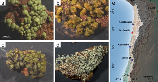
The harsh environment leads to a specialized vegetation, which is dominated by cacti (e.g., Eulychnia saint-pieana), species from the genus Euphorbia and the landscape-dominating BSCs. For an overview of the higher vegetation in the park, see [28,33]. Species of BSC change along the humidity gradient from the coastal ridge (high influence of fog) to the hinterland (more arid and less fog). At the coastal ridge, a coverage of 30% was observed mainly dominated by the four species Acarospora cf. gypsi-deserti, Caloplaca santessoniana ad int. [34], Placidium cf. velebiticum and Rinodina sp., all of which are chlorolichens.
2.2. Sampling of BSCs
The two most abundant lichen species Acarospora cf. gypsi-deserti and Caloplaca santessoniana were sampled by pressing a sterile 9-cm Petri dish 1 cm into the soil. Excess soil was removed with the Petri dish lid. Samples were air-dried in the field immediately after collection for 2–3 days, until no further condensation occurred. The dry and sealed crust samples were preserved at until further processing. For this study, the samples were slowly defrosted under air-tight conditions before they were used for the laboratory analysis.
2.3. Laboratory Analysis
CO gas exchange measurements were conducted according to [35] with the two most abundant crustose chlorolichen species Acarospora cf. gypsi-deserti and Caloplaca santessoniana with soil adhering to their rhizines. Before measurements, the intact lichen samples underwent a reactivation procedure of one day exposure at 8 in the dark. Afterward, the samples were placed in the gas exchange cuvette and sprayed with sterile, filtered water to activate their metabolism 24 h prior to measurement. Ahead of the measurements, full water saturation was achieved by submerging the samples in water for ten minutes. Excessive water and droplets were carefully shaken from the sample before measurements. CO gas exchange measurements were conducted under controlled laboratory conditions using a mini-cuvette system (GFS 3000, Walz Company, Effeltrich, Germany). The response of net photosynthesis (NP) to water content was determined for the lichens. Complete desiccation cycles (from the water-saturated phase to the air-dried status) were measured under saturating light (800 mE) and ambient CO at 24 . Samples were weighted between each measurement cycle, and the water content was calculated as mm precipitation equivalent. Sample dry weight was determined after 3 days in a drying oven (Heraeus Instruments T6P, Thermo Fischer Scientific Inc., Waltham, MA, USA) at 60 . The CO gas exchange of the samples was related to the lichens’ surface and chlorophyll content, the latter determined after [36].
2.4. Hyperspectral Measurements
Hyperspectral reflectance data have been acquired with two different instruments. In the field, a Specim ENIR hyperspectral camera (Specim, Spectral Imaging Ltd., Oulu, Finland) has been used, which acquires images consisting of 256 bands sensitive to electromagnetic radiation between 600 nm and 1600 nm. The spectral configuration allows continuously acquiring reflectance values with full-width-half-max values between 4.08 nm (red part of the electromagnetic radiation) and 4.17 in the near-infrared (NIR). In early summer in December 2017, hyperspectral samples were taken under sunny conditions close to noon to minimize bi-directional effects due to varying illumination geometries at acquisition time. The camera is a line scanner, which was mounted on a rotary stage. Rotation speed was automatically adjusted to the integration time so that a full spatial coverage of the target without overlapping pixels was achieved. To convert the raw values into reflectances, a Spectralon white standard (reflectance ≈ 95%) was arranged in the images. Sensor noise was removed by acquiring images under dark conditions immediately before and after each scan. Therefore, the lens of the camera was closed by a screw-cap. Both dark current images were averaged column-wise since noise in the instrument changes across the scanner array. Reflectance values were then calculated:
Here, is the reflectance in band and column c. are the raw count values of the sensor, and and are the averaged dark current and white standard values, respectively.
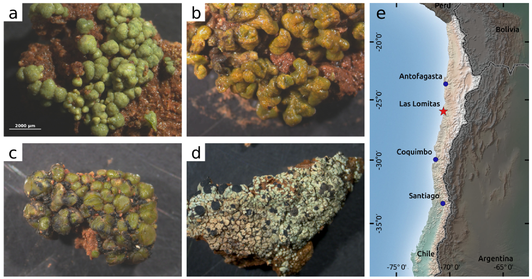
All locally-dominating species of BSCs were sampled and arranged in rows. From each species, at least 5 replicates have been sampled (Figure 2). After acquisition of the first image under dry conditions, the samples and the surrounding soil were watered. In total, seven images were acquired over a 20-min time period until the samples were visually dry, again.
The second instrument was a Spectrometer (HandySpec Field, Tec5 AG, Oberursel, Germany), which was used in the laboratory with an artificial light source. We could not use the hyperspectral camera in the laboratory because the focus range and size of the instrument did not allow properly measuring the samples in the cuvette. The spectrometer is sensitive to radiation between 305 nm and 1705 nm at a spectral resolution of 1 nm and has two channels crossing at roughly 1050 nm. To convert the raw values into reflectances, the same approach as described above has been used, and Equation (1) has been applied. At time intervals of five minutes, the samples were removed from the GFS 3000 to weigh them and to acquire hyperspectral reflectance values. At each time interval, three independent measurements were taken and averaged to reduce the effects of small movements of the sample and the measuring device. Unfortunately, the sample could not be removed from the cuvette due to fragility. This causes the radiation to interact with the plastic of the cuvette and/or the background may partly influence the absolute reflectance values measured by the spectrometer.
2.5. Hyperspectral Analysis
The hyperspectral analysis was conducted in R statistical software [37] using the raster- [38] and the hsdar-packages [39]. To remove noise from the raw spectra, a Savitzky–Golay filter has been applied (filter length of 15 and 25 bands for Specim ENIR and HandySpec Field, respectively). To cope with the different spectral configuration between the spectrometer and the hyperspectral camera, the spectra acquired with the spectrometer were resampled to the bands of the hyperspectral camera by considering Gaussian spectral response functions defined by the center and full-width-half-maximum values of the Specim ENIR sensor.
Since the spectra measured in the laboratory may be partly contaminated by background reflection, we compare two different approaches to remove artifacts arising from the measurement setup. The first one is based on normalized ratio indices (), which were calculated for all possible band combinations [40]:
Here, R is the reflectance at wavelength . It can be assumed that the spectra in the laboratory acquired with an artificial light source may differ systematically from those taken in the field. Therefore, the -values were further normalized using the dry spectra as reference:
The second approach to normalize the spectra was performed by applying continuum removal ensuring that only local differences within spectral absorption features were taken into account. We constructed a segmented continuum line to each spectrum and calculated the band depth values [41]:
Here, and denote the reflectance and continuum line value at wavelength . For each identified feature, the integral and the width between lower and upper full-width-half-maximum values have been calculated.
The relationship between water content and NP for BSC is known to be non-linear [42,43]. Therefore, species-specific second degree polynomial functions were fitted to the hyperspectral signal of Caloplaca santessoniana and Acarospora cf. gypsi-deserti and NP as the dependent variable. Independent variables were each normalized ratio index and each variable of the absorption features:
Here, x denotes the normalized ratio index or absorption feature variable. Please note that we did not directly fit models to the band depth values and that only univariate models were fitted because the indices are highly correlated. Based on the -values of the models, the model with the highest proportion of explained variance has been selected.
The normalized ratio index with the highest predictive performance regarding NP under laboratory conditions was calculated from all hyperspectral images acquired in the field. Predictive performance was compared by the -values of the models. Normalization of the index values has been performed according to the normalization of the spectrometer data by using the image acquired under dry conditions as the reference. Afterward, the species-specific models derived from the laboratory measurements were used to predict NP in the hyperspectral images. For the models with the highest proportion of explained variance derived from continuum removal variables, the same approach has been conducted.
The soil close to the BSCs was used as a control to determine whether the relationships between NP and hyperspectral signal is a consequence of the reflectance properties of the BSCs or the soil beneath the crusts. Therefore, pixels covered only by soil without any crusts have been extracted from the hyperspectral images taken in the field and processed in the same manner as for the pixels covered by BSCs.
3. Results
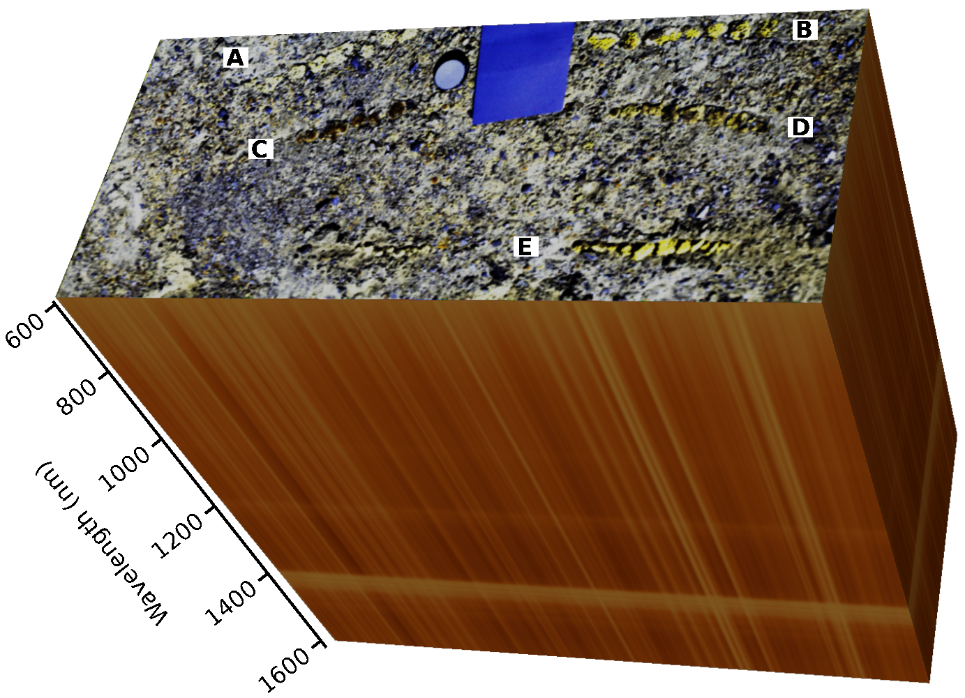
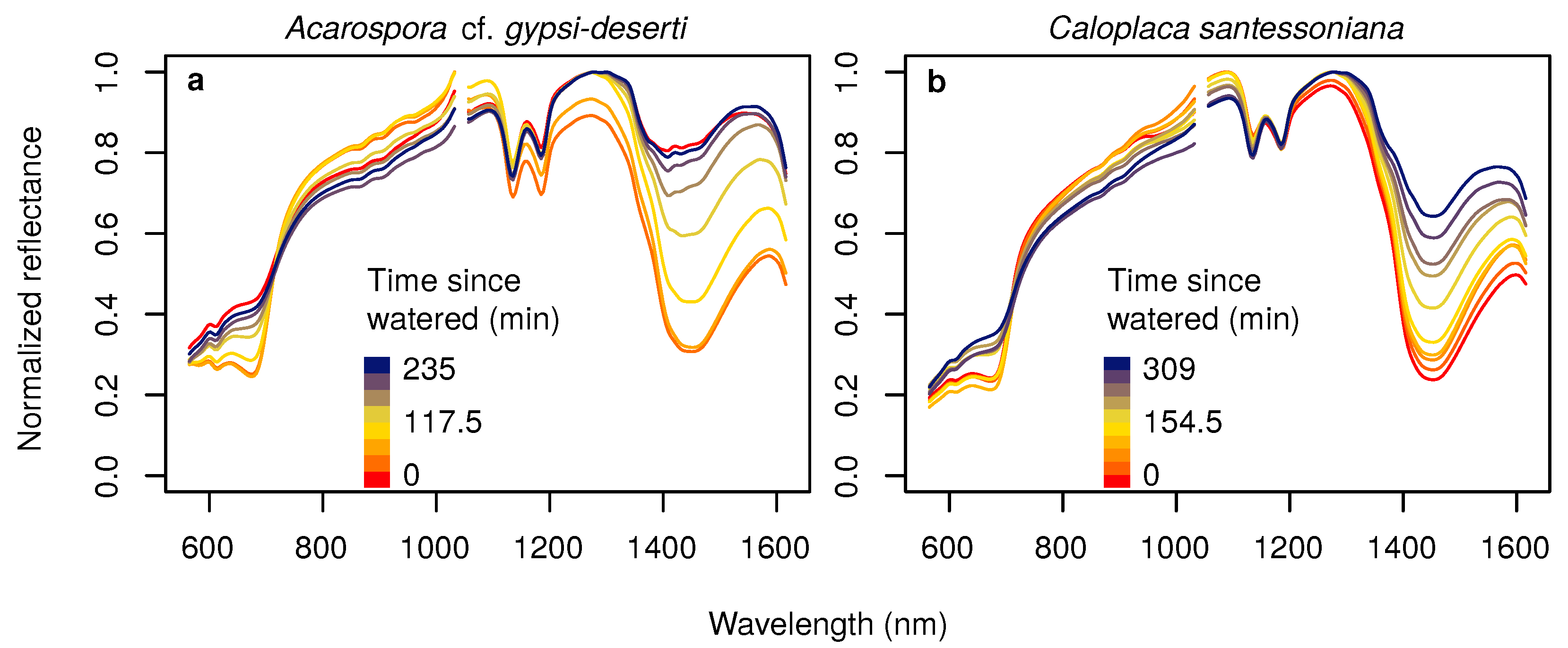
Spectra measured in the laboratory differed clearly between dry and wet stages (Figure 3). Under dry conditions, the spectra of all species were similar to typical soil spectra, because the chlorophyll absorption feature at approximately 680 nm was only marginally developed. If specimens were watered, the spectra changed immediately. The strongest differences could be observed at the chlorophyll absorption bands and at the water absorption bands around 1450 nm. Reflectance values in the NIR increased, whereas those in the red and mid-infrared decreased. The dryer the specimen became, the smaller were the spectral differences compared to the spectra acquired under initial dry conditions. After 4–5 h, the spectra were almost identical to the initial ones.
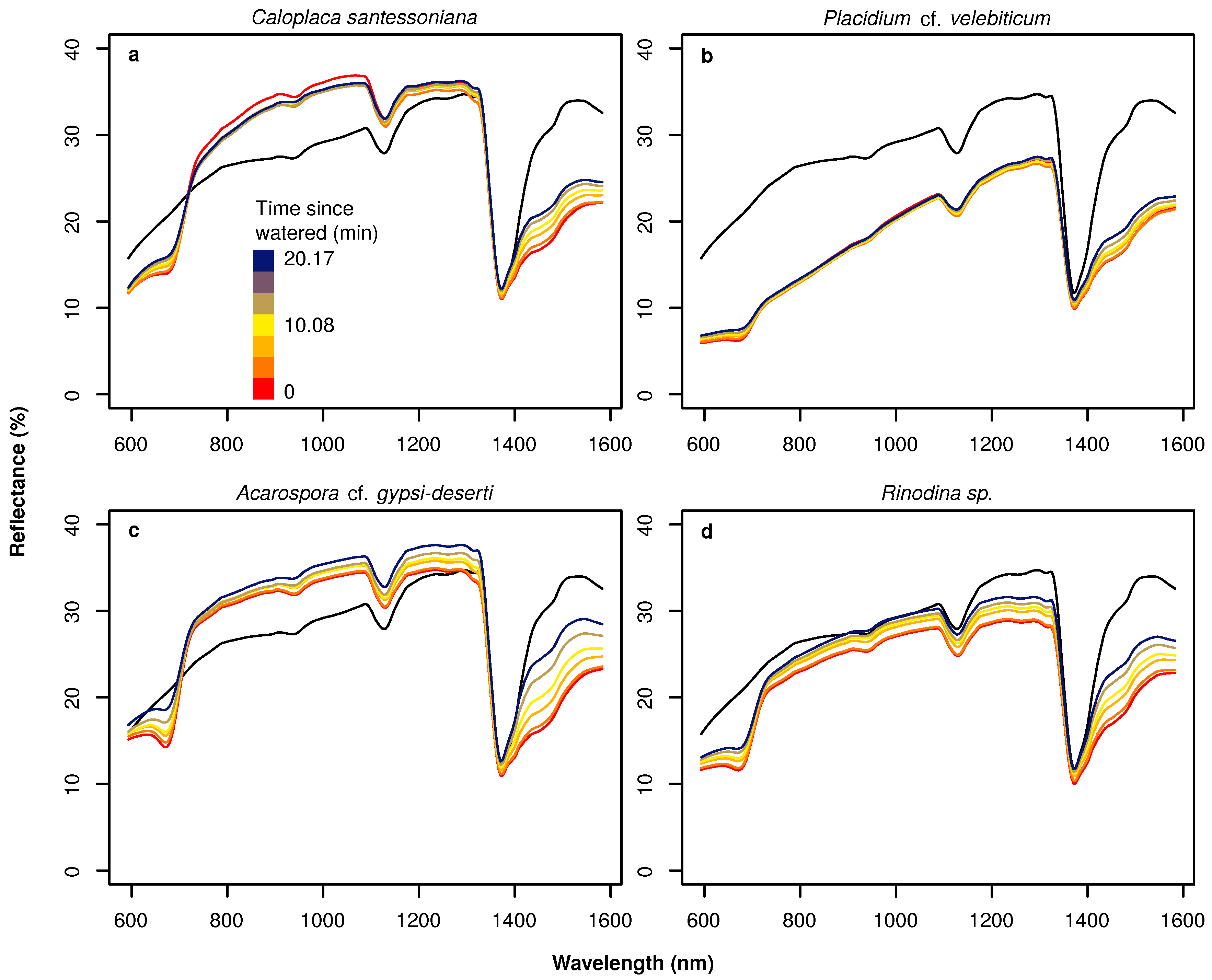
Spectra were also different between wet and dry stages if hyperspectral data were acquired under field conditions (Figure 4). Here, the pattern was less pronounced compared to the laboratory spectra. Spectral signatures of the BSC species differed from soil reflectances in terms of shape only in the red part, where the soil reflectance was characterized by a slower increase towards the NIR. Both soil and the BSC spectra had a distinct absorption feature at approximately 1150 nm. Large spectral differences were found among the BSC species. Similar reflectance values were observed for the two wide-spread species Caloplaca santessoniana and Acarospora cf. gypsi-deserti, whereas reflectances of Placidium cf. velebiticum were generally substantially lower. Additionally, no chlorophyll absorption feature could be observed for Placidium cf. velebiticum in the dry stage. Rinodina sp. was characterized by intermediately high reflectances and an intermediately developed chlorophyll absorption feature under dry conditions.
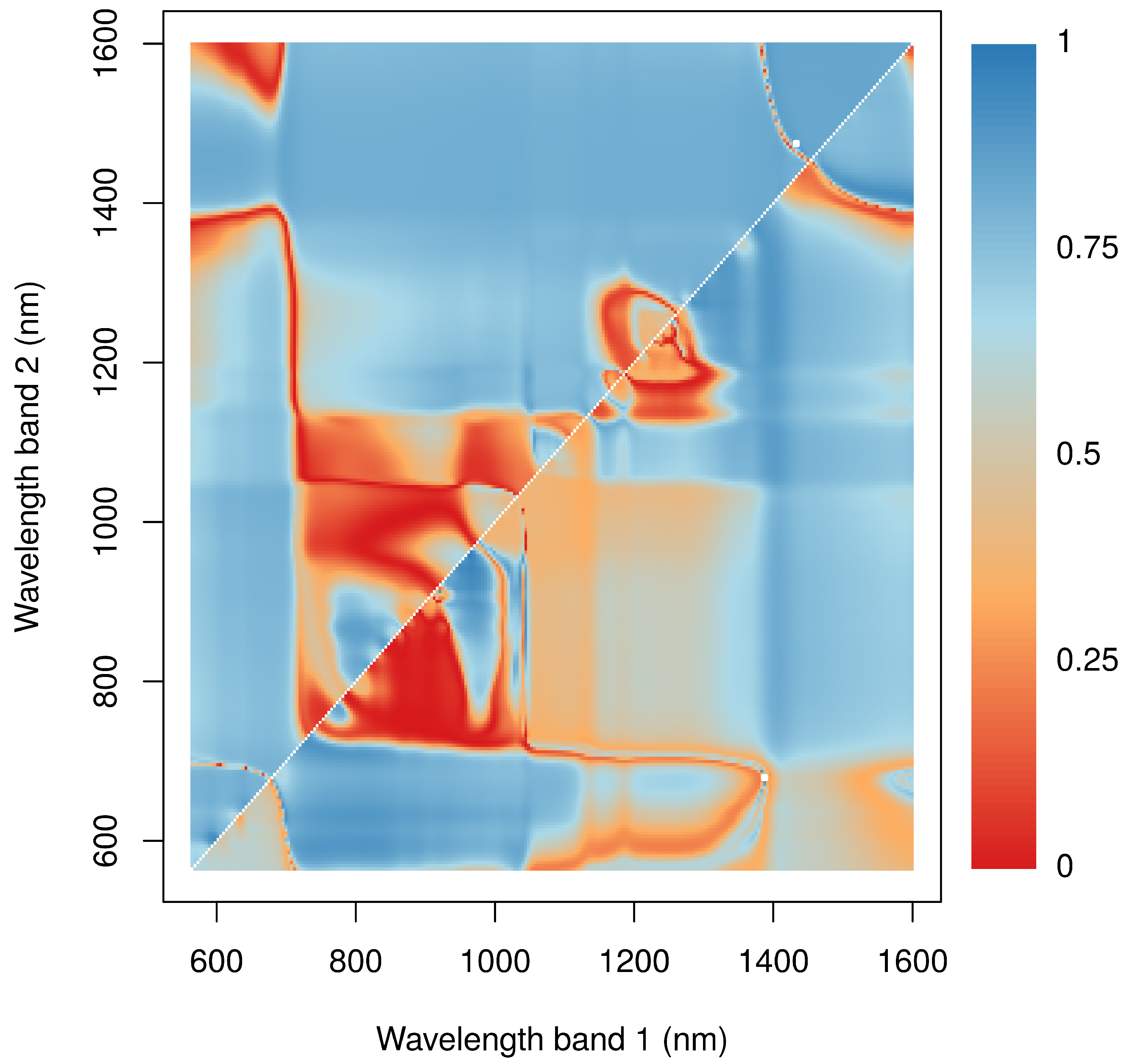
The relationship between NP and spectral reflectances was evaluated for the two most common species Caloplaca santessoniana and Acarospora cf. gypsi-deserti. Here, normalized ratio indices revealed similar patterns in both species (Figure 5). Close relationships were found for indices calculated from reflectances in the NIR including the red edge and the red part of electromagnetic radiation. Additionally, indices derived from bands at the water absorption feature at 1420 nm and any band from the NIR revealed close relationships. In contrast, band combinations from the NIR and the red-edge were not useful to estimate NP. In general, the -values were higher for Caloplaca santessoniana than Acarospora cf. gypsi-deserti. Regarding Caloplaca santessoniana, the best index was calculated from reflectance values at 1475 nm and 1433 nm, whereas the best index for Acarospora cf. gypsi-deserti used bands at wavelengths of 1388 nm and 679 nm (Table 1). Consequently, for both species, at least one band was selected from the water absorption feature around 1420 nm. For both species, differences between the best and the indices with consecutively lower explanatory power were small.
Four absorption features have been identified by applying continuum removal. The first one was the chlorophyll absorption feature at approximately 680 nm. The second and third feature were smaller and located around 950 nm and 1100 nm. The fourth one around 1420 nm was the large water absorption feature. Variables from all four absorption features have been tested for their usability to predict NP of Acarospora cf. gypsi-deserti and Caloplaca santessoniana (Table 2). The best variable for both species was the integral of the water absorption feature around 1400 nm. Additionally, the width of the absorption feature around 1400 nm performed well for the prediction of NP in Caloplaca santessoniana, but not in Acarospora cf. gypsi-deserti. All other features including the chlorophyll absorption feature around 680 nm were not useful to estimate NP of both BSC species.
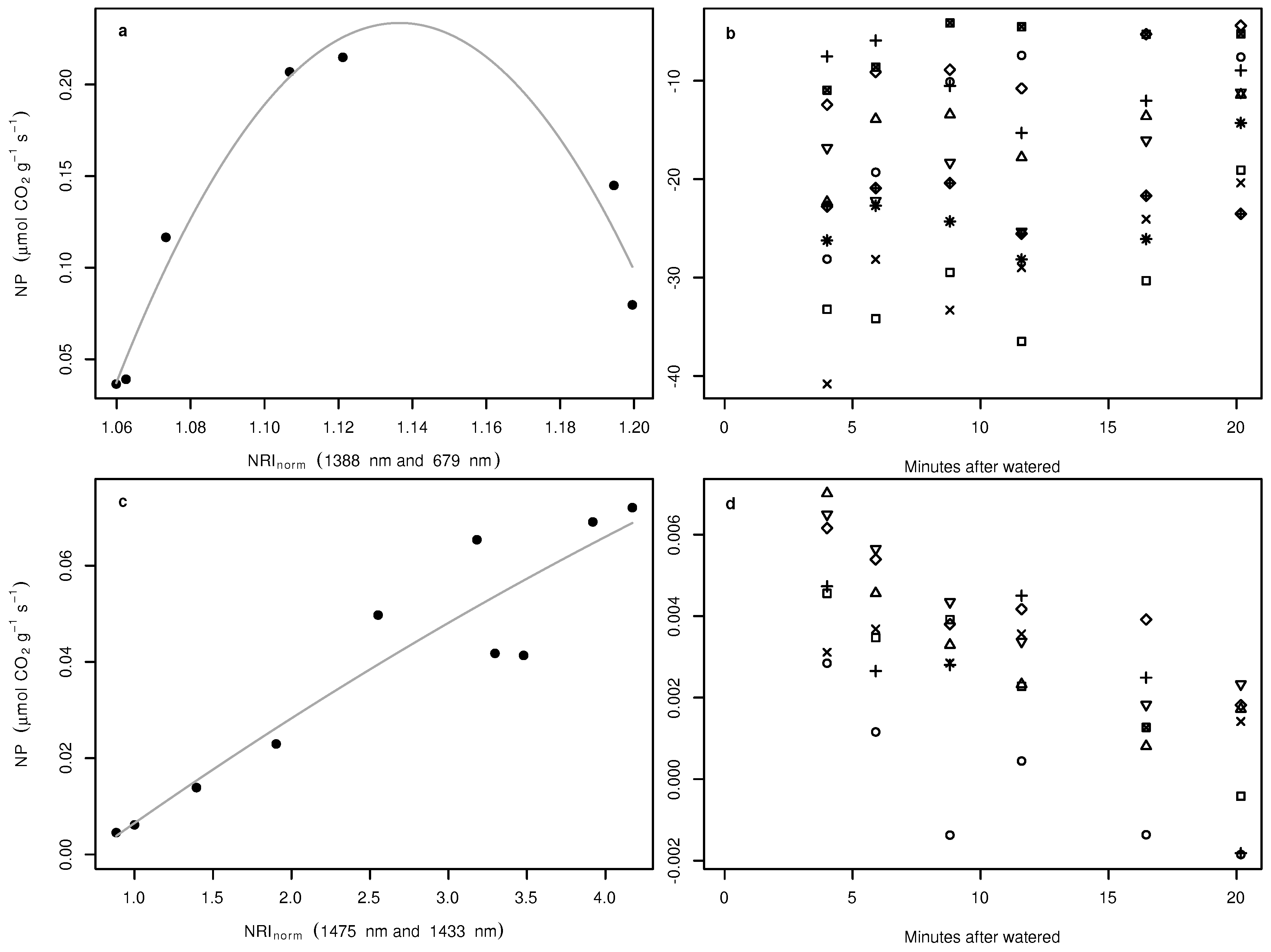
A non-linear relationship between NP and water availability was observed for Acarospora cf. gypsi-deserti (not shown). In the low and high water availability stages, NP was close to zero, and the highest NP was measured at an intermediate water content of approximately mL m. For normalized ratio indices and continuum removal, the index and the absorption feature derived variables that revealed the closest relationship to NP were tested for the applicability to the spectra acquired under field conditions. Regarding normalized ratio indices, the best index to predict NP of Acarospora cf. gypsi-deserti was derived from bands at 1388 nm and 679 nm and revealed a clearly non-linear relationship with NP (Figure 6a). In the dry and wet stages, the index values were small and large, respectively. The highest values of NP were observed for intermediate index values. If applied to spectra acquired under field conditions, no pattern within the estimates over time could be observed (Figure 6b).
For Caloplaca santessoniana, a close linear correlation was observed between NP and the water content of the sample in the laboratory. The best normalized ratio index for Caloplaca santessoniana was derived from reflectance values at 1475 nm and 1433 nm. In contrast to Acarospora cf. gypsi-deserti, the relationship was almost linear (Figure 6c). If applied to field spectra, a clear pattern was observed (Figure 6d). NP was highest directly after artificial watering of the samples in the field and decreased until the samples were visually dry. However, the highest and lowest predicted NP were one order of magnitude lower compared to the laboratory measurements.
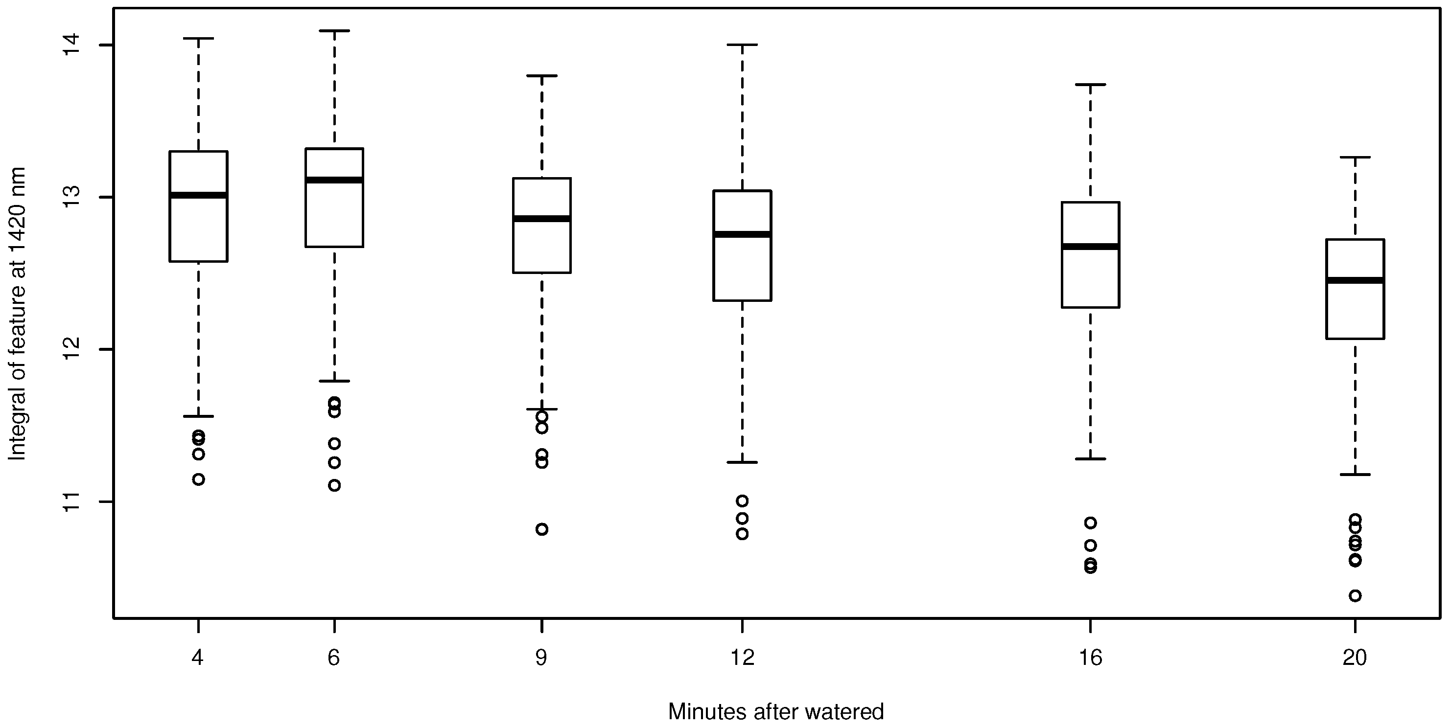
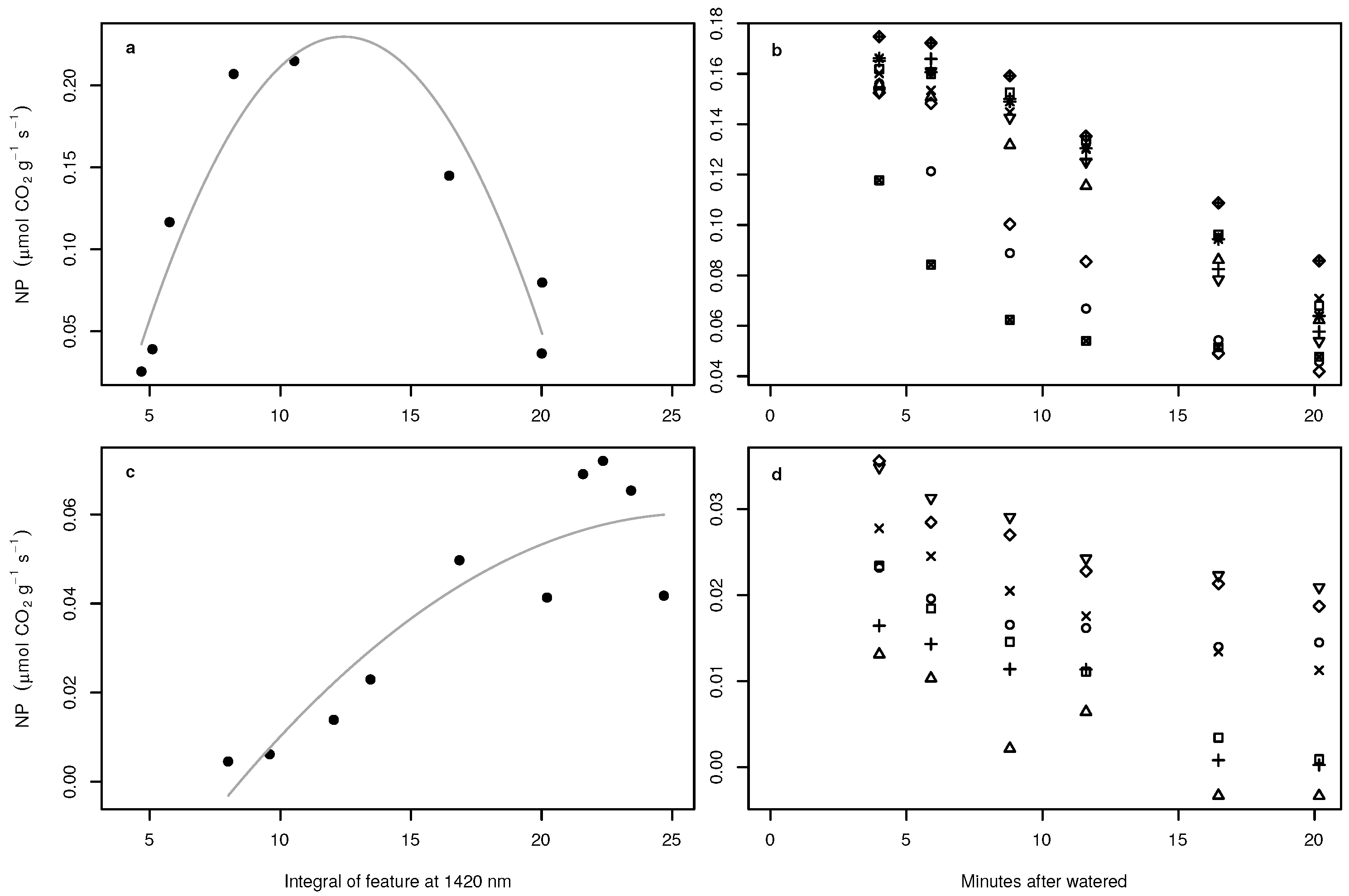
The variable derived from continuum removal with the highest predictive performance was the integral of the feature at 1420 nm for both species. To test if the relationships identified between NP and the hyperspectral signal are a consequence of the BSCs or the soil beneath the crust, the change in the integral of the absorption feature at 1420 nm for pixels covered only by soil was investigated over time (Figure 7). In general, the integral values slightly declined during drying-out of the soil. Regarding Acarospora cf. gypsi-deserti, a non-linear relationship was observed, which was similar to the relationship derived for the normalized ratio index (Figure 8a). If the empirical transfer function was applied to the field spectra, a clear pattern was observed in NP predictions (Figure 8b and Figure 9a). NP was highest in all individuals in the first image after artificial watering and decreased with progressive drying-out. The estimates were in the range of the laboratory measurements.
For Caloplaca santessoniana, the relationship was linear except one measurement causing the regression line to decrease at the higher range of the values (Figure 8c). As for Acarospora cf. gypsi-deserti, a clear pattern in the predictions of NP for the field samples was observed, which were in the range of laboratory measurements (Figure 8d and Figure 9b).
4. Discussion
We found differences in the spectral signal of different species of BSCs. Irrespective of the water content, spectral properties of Caloplaca santessoniana and Acarospora cf. gypsi-deserti were similar, whereas Rinodina sp. and Placidium cf. velebiticum were characterized by generally lower reflectance values. Water content affected the spectra of all species mainly in the water absorption bands around 1420 nm and the chlorophyll absorption feature at approximately 680 nm. The spectral signal in both absorption features changed within minutes after water became available to the BSC, which confirms the result of [44] for Australia, while NP initialization is faster than the observations reported by [12] from the Arabian Peninsula. In contrast to the results from Australia, the spectral signal was almost identical after the sample became dry both in the laboratory and the field [44]. Since the distinct spectral feature at 1120 nm is present in the soil and all BSC species, it is most likely a consequence of an andesite-rich bedrock [45]. This shows that even spectra from the laboratory samples were partly influenced by the reflection of the soil beneath the crust, which could not be completely removed from the samples.
Robust relationships between water content and NP were found for the two most wide-spread species Acarospora cf. gypsi-deserti and Caloplaca santessoniana in the laboratory. The non-linear, positively-skewed response of Acarospora cf. gypsi-deserti corresponds well to prior measurements of other species, e.g., of the genus Lecidella [42]. The fast and quasi-linear relationship between NP and water content for Caloplaca santessoniana has been observed, e.g., for genus Peltula [46]. Hyperspectral reflectances changed with the water content of the sample, which allowed deriving robust transfer functions between the NP measurements and the spectra acquired in the laboratory. In this respect, the most relevant spectral bands for NP estimation were situated in the water absorption feature at 1420 nm and the chlorophyll absorption bands. Since no direct measurements of chlorophyll activity via, e.g., chlorophyll fluorescence were available to date, it is unknown if water content or chlorophyll activity is the main influencing factor on normalized ratio indices.
The spectra in the laboratory may be contaminated partly by radiation that interacted with the plastic cuvette, because the fragile samples could not be removed for hyperspectral data acquisition. Consequently, two different normalization methods of the spectra were compared: normalized ratio indices and variables based on absorption features derived by continuum removal. Regarding the normalized ratio indices, we found that good predictors of NP for both species were derived from bands in the water absorption feature, the NIR between 1100 nm and 1300 nm and the red part lower than 700 nm. Contrasting patterns between normalized ratio indices and NP between both species were mainly found in the red-edge where NP of Acarospora cf. gypsi-deserti could not be predicted by indices derived from bands close to the shoulder of the red-edge, whereas models for Caloplaca santessoniana revealed a generally good predictability in the same spectral range. This shows that hyperspectral responses to changes in water content were partly species dependent. Since the red-edge is a frequently-used indicator for NP (e.g., via the NDVI and other vegetation indices), care must be taken that the estimates of NP from vegetation indices are validated against data from other sensors such as chlorophyll fluorescence imagers [18].
The variables derived from the absorption features defined by continuum removal had a generally lower predictive performance for NP compared to the normalized ratio indices. The only variable that was related to NP was the integral of the water absorption feature at 1420 nm. Surprisingly, no relationship between the chlorophyll absorption feature and NP was detected for either species after continuum removal. This underlines that common vegetation indices should be treated with care if they are used as predictors for chlorophyll activity of BSCs in space and time.
Irrespective of the applied normalization method, the parameters in the polynomial fits differed highly among both species as a consequence of the species-specific form of the relationship between water content and NP. This clearly shows that no universal empirical transfer function across different BSC species between NP and the hyperspectral reflectance signal can be derived. Instead, species-specific relationships at least for the most wide-spread species must be established for any estimation of NP in space and time based on remotely-sensed data in the future.
We tested whether our empirical transfer functions derived from laboratory measurements can be applied to field data even though two different sensors have been used. We found that normalized ratio indices were not useful in our case because estimates of NP based on field data differed from laboratory measurements partly by more than one magnitude. Especially for Acarospora cf. gypsi-deserti, the empirical transfer functions derived from normalized ratio indices were unable to reproduce any kind of pattern between NP and water content. One reason for the failure of normalized ratio indices for Acarospora cf. gypsi-deserti could be that differences between the samples in the field and the laboratory sample (e.g., thickness of BSC, chlorophyll content) caused the empirical transfer function to be ambivalent, because only reflectance values at two wavelengths were considered. The other factor influencing the transferability of the laboratory-derived functions to field data is the usage of two different sensors in this experiment. This was unfortunately necessary because no line scanner camera could be used in the laboratory since the focus range and size of the instrument did not allow properly measuring the samples in the cuvette. To cope with this limitation, we spectrally integrated the reflectance values of the spectrometer to the bands of the hyperspectral camera assuming Gaussian spectral response functions, because no spectral response function could be provided by the manufacturer. If this assumption is not fully valid, it may partly explain why spectral features in parts of the electromagnetic radiation with high heterogeneity (e.g., the red edge) were not useful to predict NP of BSCs in this study.
Although the predictive performance of the integral at 1420 nm was lower compared to normalized ratio indices in the laboratory spectra, the predictions of those empirical transfer functions based on field data were in astonishingly good agreement with the theoretical expectations [42]. We found that after watering in the field, hyperspectrally-predicted NP for all individuals decreased over time, which was in the range of the laboratory estimates. In the meantime, changes in the hyperspectral signal of the soil were much less pronounced compared to the BSCs. This implies that the relationships between NP and the hyperspectral signal were a consequence of the reflectance properties of the BSCs rather than the soil beneath the crust. However, it has to be noted that NP was measured under controlled laboratory conditions in this study. Consequently, the absolute predicted values based on field data must be considered carefully. Comparing the predictions between the different normalization methods, we conclude that continuum removal is a more robust technique compared to normalized ratio indices, especially under different conditions (e.g., field vs. laboratory) and when different sensors are used. Additionally, the usage of full absorption features reduces the sensitivity of the empirical transfer functions to differences among individuals such as the thickness of the BSCs.
The spatial resolution in our analysis is extremely high, which leads to the question of whether the results can be applied to data featuring lower spatial resolutions such as data acquired by satellites or aircraft. Since our transfer functions have been fitted to laboratory measurements where the entire field of view was covered by BSCs, any kind of transfer to mixed pixels is speculative. Therefore, additional investigations based on field data are required in order to verify our results for large-scale data. Irrespective of the mixed pixel effects, our finding that the most robust spectral indicator for NP of BSCs is located in the water absorption feature around 1420 nm causes severe implications if satellite or airborne hyperspectral data will be used for the investigation of NP. First, the absorption feature at 1420 nm does not only depend on the water content of the BSCs, but also on water vapor content of the atmosphere (e.g., [47]), which could be neglected in the present study because distances between the sensor and the BSCs were small. Consequently, if satellite or airborne data will be used, a proper atmospheric correction is mandatory. Taking the low signal to noise ratio of current hyperspectral sensors into account (e.g., [48]), it must be questioned if present hyperspectral satellite data are appropriate to estimate NP of BSCs in the Atacama Desert. Second, the usage of satellite data is generally restricted since the BSCs are only active for a short time after water becomes available. In the Atacama Desert, the latter strongly depends on fog input, which impedes satellite data in remotely sensing NP of BSCs, because satellite scenes of active BSCs are cloud-covered.
5. Conclusions
The aims of the present study were three-fold:
- We described for the first time the hyperspectral reflectance signal of BSCs in the Atacama Desert under different water availability conditions. Here, we could demonstrate that hyperspectral reflectance signals among wide-spread species of BSCs in the Atacama Desert differed largely, but water content affected the spectra in a similar manner. Changes in water availability immediately influenced the chlorophyll absorption bands in the visible and the water absorption bands in the near-infrared part of the electromagnetic spectrum.
- We tested the suitability of hyperspectral remote sensing data for the NP estimation of BSCs and found that the relationship between water content and NP is highly species dependent, urging the need for species-specific empirical transfer functions between NP and hyperspectral reflectance values. In this respect, the species-dependent transfer functions between the size of the water absorption feature at 1420 nm were better predictors than any variable derived from chlorophyll absorption bands.
- We tested whether the transfer function derived under laboratory conditions can be applied to hyperspectral images acquired in the field, which allows mapping NP across larger scales. Our results were in astonishingly good agreement with the theoretical expectations if the transfer function relied on the water absorption feature at 1420 nm, suggesting that the spectral patterns between laboratory and field measurements were highly comparable and underlining the general possibility for area-wide predictions in the field. However, the use of the water absorption bands limits the usability of space- and air-borne data in future applications because of the strong water absorption in the atmosphere accompanied by the low signal to noise ratio of current sensors. Therefore, we suggest using drones flying at low elevations above the ground to reduce the influence of the atmosphere on the reflectance values measured at the platform. Such kinds of data can be used to provide area-wide NP estimations of BSCs in the southern part of the Atacama Desert in the future, where BSCs are keystone organisms providing key ecosystem functions such as protection against soil erosion, weathering of nitrogen and phosphorus and dust trapping.
Author Contributions
L.W.L., P.J., W.A.O. and B.B. conducted field sampling and laboratory analysis. L.W.L. and J.B. designed the hyperspectral methodology. All authors contributed to the discussion of the results.
Funding
This research was funded by the German Science Foundation (DFG) priority research program SPP-1803 “EarthShape: Earth Surface Shaping by Biota” (project CRUSTWEATHERING: grant numbers BE1780/44-1, BU666/19-1).
Acknowledgments
We are grateful to the Chilean National Park Service (CONAF) for providing access to the sample locations and the great on-site support of our research. We thank three anonymous reviewers for their valuable suggestions on a previous version of the manuscript.
Conflicts of Interest
The authors declare no conflict of interest.
References
- Belnap, J.; Lange, O. Biological Soil Crusts: Structure, Function, and Management; Ecological Studies; Springer: Berlin/Heidelberg, Germany, 2001. [Google Scholar]
- Elbert, W.; Weber, B.; Burrows, S.; Steinkamp, J.; Büdel, B.; Andreae, M.O.; Pöschl, U. Contribution of cryptogamic covers to the global cycles of carbon and nitrogen. Nat. Geosci. 2012, 5, 459–462. [Google Scholar] [CrossRef]
- Castenholz, R.W.; Garcia-Pichel, F. Cyanobacterial Responses to UV Radiation. In Ecology of Cyanobacteria II; Springer: Dordrecht, The Netherlands, 2012; pp. 481–499. [Google Scholar]
- Harel, Y.; Ohad, I.; Kaplan, A. Activation of Photosynthesis and Resistance to Photoinhibition in Cyanobacteria within Biological Desert Crust. Plant Phys. 2004, 136, 3070–3079. [Google Scholar] [CrossRef] [PubMed] [Green Version]
- Rodriguez-Caballero, E.; Belnap, J.; Büdel, B.; Crutzen, P.J.; Andreae, M.O.; Pöschl, U.; Weber, B. Dryland photoautotrophic soil surface communities endangered by global change. Nat. Geosci. 2018, 11, 185. [Google Scholar] [CrossRef]
- Warren, S.D. Synopsis: Influence of Biological Soil Crusts on Arid Land Hydrology and Soil Stability; Ecological Studies; Springer: Berlin/Heidelberg, Germany, 2001; pp. 349–360. [Google Scholar]
- Belnap, J. The world at your feet: Desert biological soil crusts. Front. Ecol. Environ. 2003, 1, 181–189. [Google Scholar] [CrossRef]
- Reynolds, R.; Belnap, J.; Reheis, M.; Lamothe, P.; Luiszer, F. Aeolian dust in Colorado Plateau soils: Nutrient inputs and recent change in source. Proc. Nat. Acad. Sci. USA 2001, 98, 7123–7127. [Google Scholar] [CrossRef] [PubMed] [Green Version]
- Castillo-Monroy, A.P.; Maestre, F.T.; Delgado-Baquerizo, M.; Gallardo, A. Biological soil crusts modulate nitrogen availability in semi-arid ecosystems: Insights from a Mediterranean grassland. Plant Soil 2010, 333, 21–34. [Google Scholar] [CrossRef]
- Pointing, S.B.; Belnap, J. Microbial colonization and controls in dryland systems. Nat. Rev. Microbiol. 2012, 10, 551–562. [Google Scholar] [CrossRef] [PubMed]
- Bowker, M.A.; Belnap, J.; Miller, M.E. Spatial modeling of biological soil crusts to support rangeland assessment and monitoring. Rangel. Ecol. Manag. 2006, 59, 519–529. [Google Scholar] [CrossRef]
- Abed, R.M.M.; Polerecky, L.; Al-Habsi, A.; Oetjen, J.; Strous, M.; de Beer, D. Rapid Recovery of Cyanobacterial Pigments in Desiccated Biological Soil Crusts following Addition of Water. PLoS ONE 2014, 9, e112372. [Google Scholar] [CrossRef] [PubMed]
- Karnieli, A.; Tsoar, H. Spectral reflectance of biogenic crust developed on desert dune sand along the Israel-Egypt border. Int. J. Remote Sens. 1995, 16, 369–374. [Google Scholar] [CrossRef]
- Ustin, S.L.; Valko, P.G.; Kefauver, S.C.; Santos, M.J.; Zimpfer, J.F.; Smith, S.D. Remote sensing of biological soil crust under simulated climate change manipulations in the Mojave Desert. Remote Sens. Environ. 2009, 113, 317–328. [Google Scholar] [CrossRef]
- Weber, B.; Olehowski, C.; Knerr, T.; Hill, J.; Deutschewitz, K.; Wessels, D.; Eitel, B.; Büdel, B. A new approach for mapping of Biological Soil Crusts in semidesert areas with hyperspectral imagery. Remote Sens. Environ. 2008, 112, 2187–2201. [Google Scholar] [CrossRef]
- Rodríguez-Caballero, E.; Paul, M.; Tamm, A.; Caesar, J.; Büdel, B.; Escribano, P.; Hill, J.; Weber, B. Biomass assessment of microbial surface communities by means of hyperspectral remote sensing data. Sci. Total Environ. 2017, 586, 1287–1297. [Google Scholar] [CrossRef] [PubMed]
- Chamizo, S.; Stevens, A.; Canton, Y.; Miralles, I.; Domingo, F.; Van Wesemael, B. Discriminating soil crust type, development stage and degree of disturbance in semiarid environments from their spectral characteristics. Eur. J. Soil Sci. 2012, 63, 42–53. [Google Scholar] [CrossRef]
- Gypser, S.; Herppich, W.B.; Fischer, T.; Lange, P.; Veste, M. Photosynthetic characteristics and their spatial variance on biological soil crusts covering initial soils of post-mining sites in Lower Lusatia, NE Germany. Flora 2016, 220, 103–116. [Google Scholar] [CrossRef]
- Rodríguez-Caballero, E.; Escribano, P.; Olehowski, C.; Chamizo, S.; Hill, J.; Canton, Y.; Weber, B. Transferability of multi- and hyperspectral optical biocrust indices. ISPRS J. Photogramm. Remote Sens. 2017, 126, 94–107. [Google Scholar] [CrossRef]
- Escribano, P.; Palacios-Orueta, A.; Oyonarte, C.; Chabrillat, S. Spectral properties and sources of variability of ecosystem components in a Mediterranean semiarid environment. J. Arid Environ. 2010, 74, 1041–1051. [Google Scholar] [CrossRef]
- Rodríguez-Caballero, E.; Escribano, P.; Cantón, Y. Advanced image processing methods as a tool to map and quantify different types of biological soil crust. ISPRS J. Photogramm. Remote Sens. 2014, 90, 59–67. [Google Scholar] [CrossRef]
- Rodríguez-Caballero, E.; Knerr, T.; Weber, B. Importance of biocrusts in dryland monitoring using spectral indices. Remote Sens. Environ. 2015, 170, 32–39. [Google Scholar] [CrossRef]
- Hinchcliffe, G.; Bollard-Breen, B.; Cowan, D.A.; Doshi, A.; Gillman, L.N.; Maggs-Kolling, G.; de Los Rios, A.; Pointing, S.B. Advanced Photogrammetry to Assess Lichen Colonization in the Hyper-Arid Namib Desert. Front. Microbiol. 2017, 8, 2083. [Google Scholar] [CrossRef] [PubMed]
- Rozenstein, O.; Karnieli, A. Identification and characterization of Biological Soil Crusts in a sand dune desert environment across Israel Egypt border using LWIR emittance spectroscopy. J. Arid Environ. 2015, 112, 75–86. [Google Scholar] [CrossRef]
- Raggio, J.; Pintado, A.; Vivas, M.; Sancho, L.G.; Büdel, B.; Colesie, C.; Weber, B.; Schroeter, B.; Lázaro, R.; Green, T.G.A. Continuous chlorophyll fluorescence, gas exchange and microclimate monitoring in a natural soil crust habitat in Tabernas badlands, Almería, Spain: Progressing towards a model to understand productivity. Biodivers. Conserv. 2014, 23, 1809–1826. [Google Scholar] [CrossRef]
- Zhang, Y.; Chen, J.; Wang, L.; Wang, X.; Gu, Z. The spatial distribution patterns of biological soil crusts in the Gurbantunggut Desert, Northern Xinjiang, China. J. Arid Environ. 2007, 68, 599–610. [Google Scholar] [CrossRef]
- Rundel, P.W. Ecological Relationships of Desert Fog Zone Lichens. Bryologist 1978, 81, 277–293. [Google Scholar] [CrossRef]
- Rundel, P.W.; Dillon, M.O.; Palma, B. Flora and Vegetation of Pan de Azúcar National Park in the Atacama Desert of Northern Chile. Gayana Bot. 1996, 53, 295–315. [Google Scholar]
- Jordan, T.; Riquelme, R.; González, G.; Herrera, C.; Godfrey, L.; Colucci, S.; Gironás-León, J.; Gamboa, C.; Urrutia, J.; Tapia, L.; et al. Hydrological and geomorphological consequences of the extreme precipitation event of 24–26 March 2015, Chile. In Proceedings of the XIV Congreso Geologico Chileno, La Serena, Chile, 4–8 October 2015. [Google Scholar]
- Cereceda, P.; Larrain, H.; Osses, P.; Farías, A.; Egaña, I. The spatial and temporal variability of fog and its relation to fog oases in the Atacama Desert, Chile. Atmos. Res. 2008, 87, 312–323. [Google Scholar] [CrossRef]
- Cereceda, P.; Schemenauer, R.S. The Occurrence of Fog in Chile. J. Appl. Meteorol. 1991, 30, 1097–1105. [Google Scholar] [CrossRef] [Green Version]
- Lehnert, L.W.; Thies, B.; Trachte, K.; Achilles, S.; Osses, P.; Baumann, K.; Schmidt, J.; Samolov, E.; Jung, P.; Leinweber, P.; et al. A Case Study on Fog/Low Stratus Occurrence at Las Lomitas, Atacama Desert (Chile) as a Water Source for Biological Soil Crusts. Aerosol Air Q. Res. 2018, 18, 254–269. [Google Scholar] [CrossRef]
- Thompson, M.V.; Palma, B.; Knowles, J.T.; Holbrook, N.M. Multi-annual climate in Parque Nacional Pan de Azúcar, Atacama Desert, Chile. Rev. Chil. Hist. Nat. 2003, 76, 235–254. [Google Scholar] [CrossRef]
- Gaya, E.; Fernández-Brime, S.; Vargas, R.; Lachlan, R.F.; Gueidan, C.; Ramírez-Mejía, M.; Lutzoni, F. The adaptive radiation of lichen-forming Teloschistaceae is associated with sunscreening pigments and a bark-to-rock substrate shift. Proc. Nat. Acad. Sci. USA 2015, 112, 11600–11605. [Google Scholar] [CrossRef] [PubMed]
- Colesie, C.; Gommeaux, M.; Green, T.A.; Büdel, B. Biological soil crusts in continental Antarctica: Garwood Valley, southern Victoria Land, and Diamond Hill, Darwin Mountains region. Antarc. Sci. 2014, 26, 115–123. [Google Scholar] [CrossRef]
- Ronen, R.; Galun, M. Pigment extraction from lichens with dimethyl sulfoxide (DMSO) and estimation of chlorophyll degradation. Environ. Exp. Bot. 1984, 24, 239–245. [Google Scholar] [CrossRef]
- R Core Team. R: A Language and Environment for Statistical Computing; R Foundation for Statistical Computing: Vienna, Austria, 2017. [Google Scholar]
- Hijmans, R.J. Raster: Geographic Data Analysis and Modeling. R Package Version 2.5-8. 2016. Available online: https://cran.r-project.org/web/packages/raster/index.html (accessed on 6 June 2018).
- Lehnert, L.W.; Meyer, H.; Obermeier, W.A.; Silva, B.; Regeling, B.; Thies, B.; Bendix, J. Hyperspectral Data Analysis in R: The hsdar-Package. arXiv, 2018; arXiv:1805.05090. [Google Scholar]
- Sims, D.; Gamon, J. Relationships between leaf pigment content and spectral reflectance across a wide range of species, leaf structures and developmental stages. Remote Sens. Environ. 2002, 81, 337–354. [Google Scholar] [CrossRef]
- Mutanga, O.; Skidmore, A. Hyperspectral band depth analysis for a better estimation of grass biomass (Cenchrus ciliaris) measured under controlled laboratory conditions. Int. J. Appl. Earth Obs. Geoinform. 2004, 5, 87–96. [Google Scholar] [CrossRef]
- Lange, O.L.; Meyer, A.; Zellner, H.; Heber, U. Photosynthesis and Water Relations of Lichen Soil Crusts: Field Measurements in the Coastal Fog Zone of the Namib Desert. Funct. Ecol. 1994, 8, 253–264. [Google Scholar] [CrossRef]
- Evans, R.D.; Johansen, J.R. Microbiotic Crusts and Ecosystem Processes. Crit. Rev. Plant Sci. 1999, 18, 183–225. [Google Scholar] [CrossRef]
- O’Neill, A.L. Reflectance spectra of microphytic soil crusts in semi-arid Australia. Int. J. Remote Sens. 1994, 15, 675–681. [Google Scholar] [CrossRef]
- Adams, J.B. Interpretation of Visible and Near-Infrared Diffuse Reflectance Spectra of Pyroxenes and Other Rock-Forming Minerals; Academic Press: New York, NY, USA, 1975; pp. 91–116. [Google Scholar]
- Büdel, B.; Vivas, M.; Lange, O.L. Lichen species dominance and the resulting photosynthetic behavior of Sonoran Desert soil crust types (Baja California, Mexico). Ecol. Proc. 2013, 2, 6. [Google Scholar] [CrossRef] [Green Version]
- Gao, B.C.; Goetz, A.F.H.; Wiscombe, W.J. Cirrus cloud detection from Airborne Imaging Spectrometer data using the 1.38 μm water vapor band. Geophys. Res. Lett. 1993, 20, 301–304. [Google Scholar] [CrossRef]
- Pengra, B.W.; Johnston, C.A.; Loveland, T.R. Mapping an invasive plant, Phragmites australis, in coastal wetlands using the EO-1 Hyperion hyperspectral sensor. Remote Sens. Environ. 2007, 108, 74–81. [Google Scholar] [CrossRef]
Figure 1.
Images of wet biological soil crusts (BSCs): (a) Acarospora cf. gypsi-deserti, (b) Caloplaca santessoniana ad int. [34], (c) Placidium cf. velebiticum and (d) Rinodina sp. The map shows the sampling location (red star) near Las Lomitas in Chile (e).
Figure 1.
Images of wet biological soil crusts (BSCs): (a) Acarospora cf. gypsi-deserti, (b) Caloplaca santessoniana ad int. [34], (c) Placidium cf. velebiticum and (d) Rinodina sp. The map shows the sampling location (red star) near Las Lomitas in Chile (e).

Figure 2.
Example hyperspectral cube with false-color composite constructed from bands at 970 nm (red), 875 nm (green) and 600 nm (blue). Round structures (partly greenish depending on the species) are biological soil crusts. Samples of the locally-dominating species were manually arranged in rows: A: Acarospora cf. gypsi-deserti, B: Caloplaca santessoniana, C: Placidium cf. velebiticum, D: Rinodina sp., E: Stereocaulon sp. The blue rectangle and circle are the gray and white standards, respectively, used to convert the raw count values to reflectances. The third dimension symbolizes the reflectance values in all spectral bands by the color of the pixels at the edge of the image. High and low reflectance values are indicated by reddish/brownish and yellow colors, respectively.

Figure 3.
Hyperspectral reflectance of Acarospora cf. gypsi-deserti (a) and Caloplaca santessoniana (b) in the dry condition (red) and after being artificially watered in the laboratory (orange to blue colors), measured with the spectrometer.
Figure 3.
Hyperspectral reflectance of Acarospora cf. gypsi-deserti (a) and Caloplaca santessoniana (b) in the dry condition (red) and after being artificially watered in the laboratory (orange to blue colors), measured with the spectrometer.

Figure 4.
Hyperspectral reflectance of soil (black) and biological soil crust species Caloplaca santessoniana (a), Placidium cf. velebiticum (b), Acarospora cf. gypsi-deserti (c) and Rinodina sp. (d) in the dry condition (red) and after being artificially watered in the field (orange to blue colors), measured with the hyperspectral camera.

Figure 5.
Relationship between NP of Acarospora cf. gypsi-deserti (lower right portion of the graph) and Caloplaca santessoniana (upper left portion) and normalized ratio indices. Colors represent the -values of the regression models between NP and values. and are indicated by the x- and y-axis. The white squares mark the position of the index that results in the highest -value.

Figure 6.
Relationships between NP of Acarospora cf. gypsi-deserti in the laboratory and the index with the highest proportion of explained variance (a). The grey curve symbolizes the regression of the polynomial fit. Predicted NP of Acarospora cf. gypsi-deserti in the field in relation to the time passed since being watered (b). Symbols in (b) indicate individuals. Note that time is always the end time of the scan process, which took about 11 s for the entire image. (c,d) show the same, but for Caloplaca santessoniana.

Figure 7.
Relationship between the integral of the absorption feature at 1420 nm for pixels covered by soil without BSCs (n = 567). The boxplots indicate the upper and the lower whisker by the horizontal lines. Boxes represent the first and third quartile, and the bold line is the median. Outliers are indicated by the open circles.

Figure 8.
Relationship between NP of Acarospora cf. gypsi-deserti and the integral of the absorption feature at 1420 nm (a). The grey curve symbolizes the regression of the polynomial fit. Predicted NP of Acarospora cf. gypsi-deserti in the field in relation to the time passed since being watered (b). Symbols in (b) indicate individuals. Note that time is always the end time of the scan process, which took about 11 s for the entire image. (c,d) show the same, but for Caloplaca santessoniana.

Figure 9.
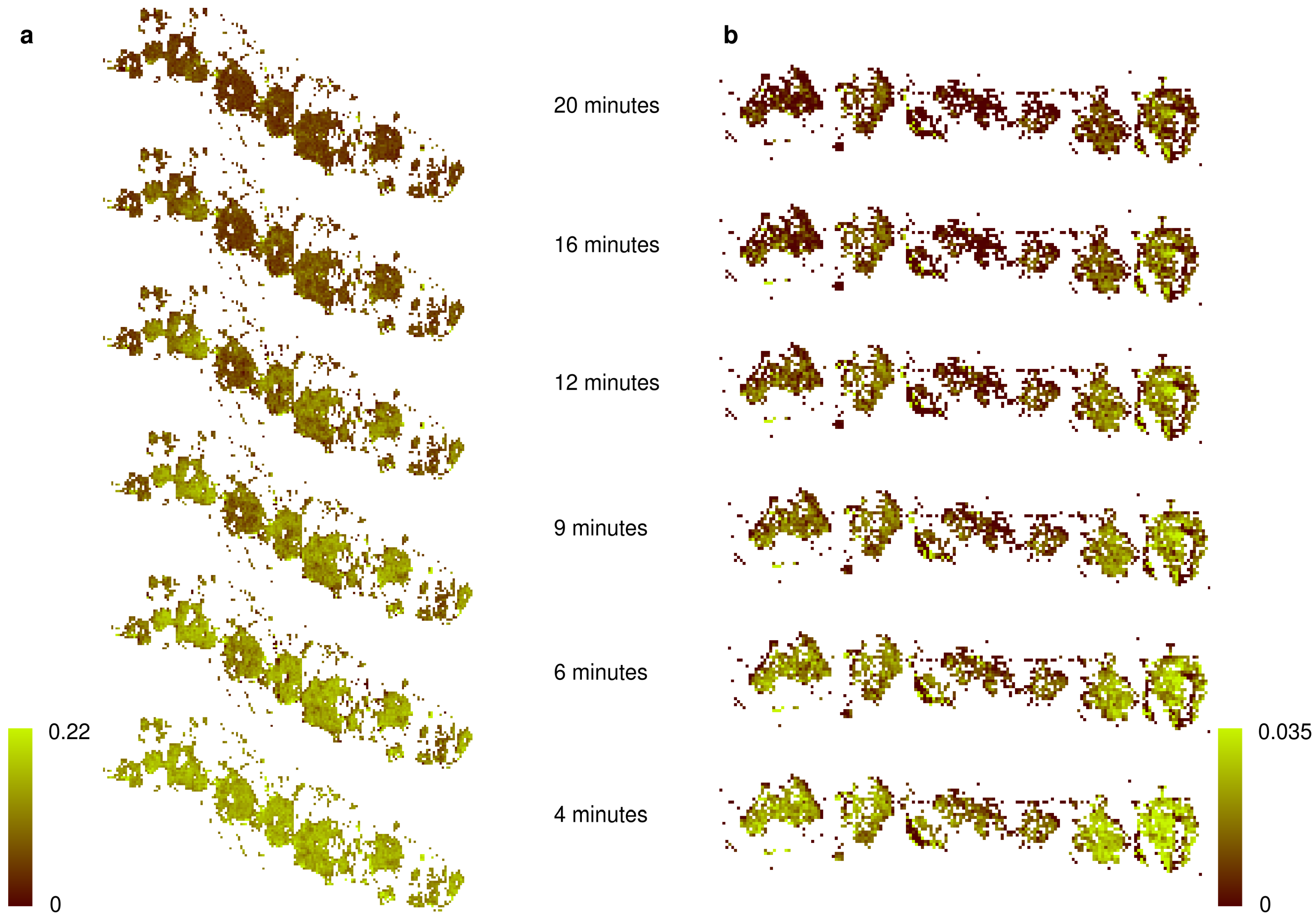
Predictions of NP in mol CO g s based on hyperspectral field data for Acarospora cf. gypsi-deserti (a) and Caloplaca santessoniana (b) during drying-out. Time is given in minutes after the BSCs have been watered.
Figure 9.
Predictions of NP in mol CO g s based on hyperspectral field data for Acarospora cf. gypsi-deserti (a) and Caloplaca santessoniana (b) during drying-out. Time is given in minutes after the BSCs have been watered.


Table 1.
Summary of the 10 best models for Acarospora cf. gypsi-deserti and Caloplaca santessoniana between NP and normalized ratio indices.
Table 1.
Summary of the 10 best models for Acarospora cf. gypsi-deserti and Caloplaca santessoniana between NP and normalized ratio indices.
| Species | NRI | Polynomial Regression | ||||
|---|---|---|---|---|---|---|
| Acarospora cf. gypsi-deserti | 1388 | 679 | −43.0170 | 76.1124 | −3.3 × 10 | 0.95 |
| 1388 | 675 | −43.4680 | 76.8389 | −3.4 × 10 | 0.95 | |
| 970 | 929 | −0.8014 | 2.9343 | −2.1 × 10 | 0.94 | |
| 966 | 925 | −0.8759 | 3.0839 | −2.2 × 10 | 0.93 | |
| 974 | 933 | −0.8830 | 3.1640 | −2.3 × 10 | 0.93 | |
| 970 | 925 | −1.0468 | 3.5271 | −2.5 × 10 | 0.93 | |
| 966 | 921 | −1.2512 | 3.9865 | −2.7 × 10 | 0.93 | |
| 970 | 921 | −1.4212 | 4.4215 | −3.0 × 10 | 0.93 | |
| 1599 | 1404 | −0.2212 | 0.1737 | −1.8 × 10 | 0.93 | |
| 979 | 937 | −1.0409 | 3.5662 | −2.6 × 10 | 0.93 | |
| Caloplaca santessoniana | 1475 | 1433 | −0.0172 | 0.0247 | −9.7 × 10 | 0.88 |
| 1599 | 1392 | 0.0254 | −0.0183 | −3.3 × 10 | 0.88 | |
| 1595 | 1392 | 0.0225 | −0.0151 | −3.3 × 10 | 0.88 | |
| 1106 | 1057 | 0.0809 | −0.1292 | 5.2 × 10 | 0.87 | |
| 1579 | 1396 | 0.0028 | 0.0050 | −4.1 × 10 | 0.87 | |
| 1554 | 1392 | 0.0540 | −0.0747 | 3.2 ×10 | 0.87 | |
| 1479 | 1429 | −0.0128 | 0.0206 | −7.3 × 10 | 0.87 | |
| 1574 | 1396 | 0.0021 | 0.0060 | −6.2 × 10 | 0.87 | |
| 1583 | 1396 | 0.0034 | 0.0041 | −2.8 × 10 | 0.87 | |
| 1591 | 1392 | 0.0201 | −0.0126 | −3.1 × 10 | 0.87 | |
Table 2.
Summary of the models for Acarospora cf. gypsi-deserti and Caloplaca santessoniana between net photosynthesis (NP) and continuum removal derived variables.
Table 2.
Summary of the models for Acarospora cf. gypsi-deserti and Caloplaca santessoniana between net photosynthesis (NP) and continuum removal derived variables.
| Species | Variable | Absorption Feature | Polynomial Regression | |||
|---|---|---|---|---|---|---|
| a | b | c | ||||
| Acarospora cf. gypsi-deserti | Integral | 0.040 | 0.1226 | −0.0412 | 0.150 | |
| −0.121 | 0.9825 | −0.8627 | 0.561 | |||
| 1.061 | −1.8794 | 0.8985 | 0.246 | |||
| −0.254 | 0.3645 | −0.0687 | 0.880 | |||
| Width | 0.302 | −0.0478 | −0.1503 | 0.444 | ||
| −0.311 | 1.3344 | −0.9299 | 0.361 | |||
| −0.026 | 0.2143 | −0.0741 | 0.041 | |||
| −43.513 | 83.7620 | −40.1740 | 0.333 | |||
| Caloplaca santessoniana | Integral | 0.030 | 0.0499 | −0.0347 | 0.127 | |
| 0.053 | −0.0024 | −0.0047 | 0.197 | |||
| −0.267 | 0.2835 | −0.0184 | 0.743 | |||
| −0.072 | 0.0816 | −0.0126 | 0.817 | |||
| Width | 0.166 | −0.2188 | 0.0727 | 0.719 | ||
| 0.158 | −0.2657 | 0.1168 | 0.396 | |||
| −0.179 | 0.3029 | −0.0979 | 0.626 | |||
| −3.354 | 5.9404 | −2.5865 | 0.799 | |||
© 2018 by the authors. Licensee MDPI, Basel, Switzerland. This article is an open access article distributed under the terms and conditions of the Creative Commons Attribution (CC BY) license (http://creativecommons.org/licenses/by/4.0/).
Share and Cite
MDPI and ACS Style
Lehnert, L.W.; Jung, P.; Obermeier, W.A.; Büdel, B.; Bendix, J. Estimating Net Photosynthesis of Biological Soil Crusts in the Atacama Using Hyperspectral Remote Sensing. Remote Sens. 2018, 10, 891. https://doi.org/10.3390/rs10060891
AMA Style
Lehnert LW, Jung P, Obermeier WA, Büdel B, Bendix J. Estimating Net Photosynthesis of Biological Soil Crusts in the Atacama Using Hyperspectral Remote Sensing. Remote Sensing. 2018; 10(6):891. https://doi.org/10.3390/rs10060891
Chicago/Turabian StyleLehnert, Lukas W., Patrick Jung, Wolfgang A. Obermeier, Burkhard Büdel, and Jörg Bendix. 2018. "Estimating Net Photosynthesis of Biological Soil Crusts in the Atacama Using Hyperspectral Remote Sensing" Remote Sensing 10, no. 6: 891. https://doi.org/10.3390/rs10060891
Note that from the first issue of 2016, this journal uses article numbers instead of page numbers. See further details here.