A Multisensor Approach to Global Retrievals of Land Surface Albedo
by
 , , , , and
Aku Riihelä
1,* ,
,
Terhikki Manninen
1,
Jeffrey Key
2,
Qingsong Sun
3,
Melanie Sütterlin
4,
Alessio Lattanzio
5 and
Crystal Schaaf
3 1
Finnish Meteorological Institute, Erik Palménin aukio 1, FI-00560 Helsinki, Finland
2
National Oceanic and Atmospheric Administration (NOAA), 1225 West Dayton Street, Madison, WI 53706, USA
3
School for the Environment, University of Massachusetts Boston, Boston, MA 02125, USA
4
University of Bern, Institute of Geography, Hallerstrasse 12, 3012 Bern, Switzerland
5
EUMETSAT, Eumetsat Allee 1, D-64295 Darmstadt, Germany
*
Author to whom correspondence should be addressed.
Remote Sens. 2018, 10(6), 848; https://doi.org/10.3390/rs10060848
Submission received: 28 March 2018
/
Revised: 7 May 2018
/
Accepted: 23 May 2018
/
Published: 29 May 2018
(This article belongs to the Special Issue Remote Sensing of Essential Climate Variables and Their Applications)
Abstract
:Satellite-based retrievals offer the most cost-effective way to comprehensively map the surface albedo of the Earth, a key variable for understanding the dynamics of radiative energy interactions in the atmosphere-surface system. Surface albedo retrievals have commonly been designed separately for each different spaceborne optical imager. Here, we introduce a novel type of processing framework that combines the data from two polar-orbiting optical imager families, the Advanced Very High-Resolution Radiometer (AVHRR) and Moderate Resolution Imaging Spectroradiometer (MODIS). The goal of the paper is to demonstrate that multisensor albedo retrievals can provide a significant reduction in the sampling time required for a robust and comprehensive surface albedo retrieval, without a major degradation in retrieval accuracy, as compared to state-of-the-art single-sensor retrievals. We evaluated the multisensor retrievals against reference in situ albedo measurements and compare them with existing datasets. The results show that global land surface albedo retrievals with a sampling period of 10 days can offer near-complete spatial coverage, with a retrieval bias mostly comparable to existing single sensor datasets, except for bright surfaces (deserts and snow) where the retrieval framework shows degraded performance because of atmospheric correction design compromises. A level difference is found between the single sensor datasets and the demonstrator developed here, pointing towards a need for further work in the atmospheric correction, particularly over bright surfaces, and inter-sensor radiance homogenization. The introduced framework is expandable to include other sensors in the future.

1. Introduction
During the 40 years of satellite remote sensing, great strides have been made towards accurate retrievals of shortwave hemispherical reflectance at the Earth’s surface, commonly known as surface albedo. Surface albedo is one of the Essential Climate Variables (ECV), as defined by the Global Climate Observing System (GCOS) [1]. Early efforts in the field relied on relatively simple methods such as seeking minima in observed Top-of-Atmosphere (TOA) reflectances (for example, Reference [2]). The importance of accounting for the directional reflectance signatures of natural terrain types was soon identified [3], paving the way for multiangular albedo calculation algorithms. Advances in numerical computational capability and radiative transfer (RT) theory enabled the application of increasingly sophisticated methods to detect clouds and correct for atmospheric scattering and absorption in satellite imagery [4,5]. This progress lead towards the first dedicated albedo algorithms and data sets with global coverage [6,7,8,9], with parallel advances in focused regional albedo mapping [10,11].
The advent of modern sensors such as the Moderate Resolution Imaging Spectroradiometer (MODIS) and Clouds and the Earth’s Radiant Energy System (CERES), with improved radiometric accuracy and spectral coverage, enabled still further advances in the estimation of surface albedo [12,13]. Many of the most recent developments in the field have been aimed towards the production of multi-decadal datasets [14,15,16], where the intercalibration of contributing instruments becomes a significant concern [17,18].
The process of deriving a surface albedo estimate out of satellite-observed radiances is complex; problems of cloud masking, atmospheric impact on observed TOA radiances, surface anisotropy, the frequency of observations, and the limited sensor spectral coverage of the shortwave wavelengths all need to be solved satisfactorily for a high-quality retrieval. Currently, multispectral thresholding methods are the standard for cloud identification and masking, but methods based on probabilistic techniques such as the Bayesian approach or optimal estimation theory are emerging [19,20]. Atmospheric correction is typically performed with precomputed Look-Up-Tables (LUT) from fully resolved RT model runs, with the associated atmospheric composition either determined a priori or potentially obtained from the instrument data itself if sufficient spectral coverage exists [21]. Algorithms for simultaneous retrievals of surface albedo and atmospheric constituents (for example, aerosol loading) have also been developed for geostationary imagers [22]. Accounting for surface anisotropy is generally done with either finding a best-fit solution between temporally aggregated and weighted multiangular satellite observations and a model for the surface’s Bidirectional Reflectance Distribution Function (BRDF) [23,24], or by using a priori defined BRDF models specific to different land cover types to correct for the surface anisotropy in each satellite observation according to the land cover it represents [14].
Owing to the challenging nature of the task and the varying characteristics of different optical satellite sensors, the traditional approach has been to treat each sensor or family of sensors separately and derive individual algorithms for each [25], although some multisensor-based methods have been proposed [26,27,28]. Some of the recent efforts in the field are also moving in the direction of extending modern optical imager records backward with older sensor data within a single processing system [15,16].
We propose a new type of approach to the problem by creating a set of methods to combine multiple satellite sensor data within a single retrieval algorithm for broadband bi-hemispherical surface reflectance, hereafter simply ‘surface albedo’. We address the problems mentioned above, in addition to new challenges such as spectral matching of the instrument channel wavebands. The envisaged advantage gained by the new approach is a substantial increase in the sampling of multiangular surface reflectances over a particular time period. Thus, a robust surface albedo estimation should become possible with a shorter sampling period than the current state of the art, enabling the tracking of higher-frequency changes in the surface. Here, for demonstration purposes, our goal is to estimate global land surface albedo with an aggregation period of 10 days.
Furthermore, our proposed methods are general enough that, in principle, the retrieval could be enhanced further by ingesting data from additional spaceborne optical imagers. The long-term goal here is to enable long-term albedo datasets to be produced. Therefore, the framework is designed around a basis of older satellite sensors, to be augmented with more modern instruments according to availability. This work has been undertaken as a pilot project of the Sustained, Coordinated Processing of Environmental Satellite Data for Climate Monitoring (SCOPE-CM), a World Meteorological Organization (WMO)-sponsored network working towards a traceable and robust generation of Climate Data Records (CDR). Henceforth, the acronym SCM refers to the data and algorithms of this framework.
In this proof-of-concept study, we combined the Advanced Very High-Resolution Radiometer (AVHRR) Global Area Coverage (GAC) observations with subsampled Moderate Resolution Imaging Spectroradiometer (MODIS) observations (MOD02SSH, collection V006) to estimate global land surface albedo. To produce a demonstrator dataset for the purposes of this paper, the combined algorithm was applied globally for July–December 2010. To prove the value of our concept, we have evaluated the obtained albedo over several Baseline Surface Radiation Network (BSRN) tower-based surface albedo measurement sites [29]. We also compared the obtained albedo estimates against established single-sensor datasets such as the MCD43 V006 [12,30,31] for MODIS and CLARA-A2-SAL [32] for AVHRR.
We begin by introducing the framework and its constituent parts (algorithms) and describe how each of them addresses a specific issue in the joint retrieval. This is followed by a brief recap of the main characteristics and limitations of both the AVHRR and MODIS observations. We then present the retrieved surface albedo and its evaluation against reference in situ measurements, and an intercomparison against state of the art datasets. Following a discussion regarding the results achieved, we finish with the conclusions of this study.
2. Data and Methods
The creation of the joint AVHRR-MODIS surface albedo retrieval framework is based on two basic principles. First, the framework should be built on existing, peer-reviewed, and proven component algorithms and input data. Second, the implementation of said algorithms should be as flexible and generic as possible. In the following, we describe the input data and the processing methods.
2.1. Satellite Data Sources
The AVHRR-GAC radiance data applied here are from the Level-2 overpasses of the Pathfinder Atmospheres—Extended (PATMOS-x) dataset, version 5.3 [33]. The dataset is a Fundamental Climate Data Record (FCDR) of the AVHRR instrument, in which calibration differences and drift between the various NOAA satellites carrying the AVHRR instrument have been compensated for [17]. The PATMOS-x subset employed here covers days of year (DOY) 180–350 of the year 2010, with data available from the AVHRR sensors onboard the NOAA-15, -18, -19, and Metop-A satellites. The AVHRR imaging channels 1 (0.58–0.68 μm) and 2 (0.725–1.00 μm) are processed. The Global Area Coverage (GAC) data record is typically considered to have a nominal spatial resolution of roughly 4 km at nadir, although the issue is complicated by the GAC sampling scheme, where four out of every five samples along the scan line are used to compute one average value, and the data from only every third scan line are processed, implying an actual resolution of 1.1 by 4 km at nadir. Cloud-free scenes (cloud probability ≤ 0.1) are identified by applying the PATMOS-x cloud mask provided with the radiance data [19]. Any pixels marked with poor quality flags (that is, bad pixel mask) are discarded.
For the MODIS radiance inputs, we use the Collection V006 Terra and Aqua Level 1B Subsampled Calibrated Radiance 5 km data (MOD02SSH & MYD02SSH; http://dx.doi.org/10.5067/MODIS/MOD02SSH.006). We choose to use the subsampled MODIS data to obtain comparably sized sensor footprints from both AVHRR and MODIS for the (downscaling) reprojection into a common grid for atmospheric correction and albedo estimation. Cloud-free scenes are identified with the cloud mask obtained from the Collection-6 MODIS Atmosphere Level 2 Joint Product (MOD02ATML & MYD02ATML) [34]. Specifically, we obtain the cloud mask corresponding to quality flags of ‘Determined Cloud Mask, Confident Clear, Day’. Terra and Aqua overpass data from imaging channels 1 (0.62–0.67 μm) and 2 (0.841–0.876 μm), covering the days of year (DOY) 180–350 of the year 2010, are utilized.
2.2. The Pipeline: Algorithms for Joint AVHRR-MODIS Albedo Retrievals
The processing flow for the joint surface albedo retrieval is illustrated in Figure 1. The applied philosophy is that of a single pipeline. We first spectrally adjust MODIS reflectances to be ‘AVHRR-like’, then atmospherically correct all overpasses with a single correction algorithm with spatially and temporally resolved the atmospheric composition inputs. We then feed all valid data into the RossThick-LiSparse-Reciprocal Bidirectional Reflectance Distribution Function (BRDF) inversion algorithm [23] which resolves the BRDF kernel weights. With the resolved kernel weights for isotropic, geometric, and volume scattering, the desired albedo quantities may then be calculated following the MODIS methodology [12]. In the following, we describe each of the steps in more detail.
2.3. Spectral Homogenization and Reprojection
MODIS and AVHRR both observe the Earth near daily, but at different wavebands. While channel 1 is highly similar between the instruments (previous section), channel 2 is much narrower in MODIS than in AVHRR. Therefore, a spectral homogenization of the input reflectance data is required before joint use. A method to do this was developed by Manninen et al. [35]. It is based on statistically analyzing and correlating large numbers of TOA reflectance distributions observed by both MODIS and AVHRR, requiring neither Simultaneous Nadir Overpasses (SNOs) nor simultaneous observations in general. The method yields a set of linear coefficients for adjusting the MODIS TOA reflectances to resemble AVHRR, as shown in Equations (1) and (2):
where reflectances in the two channels, CH1 and CH2, are in the range 0–100%. It is worth noting that the coefficient values are a function of the AVHRR and MODIS FCDR used; any recalibration or use of a different version of the input datasets would require new coefficients to be computed. The coefficients shown are used for all surface types, which may introduce minor uncertainty in the output [35,36]. Post-adjustment, AVHRR still tends to overestimate MODIS by about 2% in channel 1 and 6% in channel 2 [35]. However, considering the AVHRR instrument accuracy limitations (often estimated at about 3–5%), the adjustment method has been evaluated and shown to achieve its goal of making MODIS observations ‘AVHRR-like’ (obtained R2 of 0.976 for CH1 and 0.948 for CH2 in a weighted Deming regression between AVHRR and MODIS [35]). Of note is that the largest relative spectral difference between AVHRR and MODIS of major land cover types occurs in CH2 for snow and vegetation [35]. The relative spectral difference in CH1 is large for vegetation, but the small vegetation reflectance in CH1 diminishes its impact.
At this stage, all observations marked as cloudy, probably cloudy, or otherwise of poor quality are discarded. Additionally, all observations where either the Sun or View Zenith Angle (θs, θv, respectively) exceed 70 degrees are discarded, as atmospheric corrections are highly challenging for very long atmospheric path lengths on the one hand, and the geolocation errors may be very large for edge-of-swath pixels on the other. Imagery marked as having θs between 60 and 70 degrees, sun glint conditions, or ‘probably clear’ cloud mask flag are kept, but penalized in the BRDF inversion. See relevant section below for details.
After the spectral matching step, all input data are re-projected to a common 0.1-degree latitude-longitude grid via nearest-neighbor matching, with a 10 km radius search for matches at each grid cell. While MODIS geolocation is generally precise, AVHRR geolocation suffers from several issues which may lead to occasionally misplaced pixels even when downscaling the resolution to 0.1 degrees [37] (and references therein). While these misplaced observations add unwanted noise to the best-fit BRDF inversion, they do not invalidate its use. The use of a downscaled processing resolution also allows us to ameliorate spatial coverage issues stemming from the inhomogeneous AVHRR-GAC sampling.
2.4. Atmospheric Correction
The atmospheric correction of the (spectral) TOA reflectances to surface reflectances utilizes the 6S radiative transfer model [38,39] via the Py6S software library [40]. The 6S model is very accurate but computationally expensive for large data such as ours. Therefore, look-up-tables (LUT) were precomputed for channels 1 and 2 to parameterize the correction for a range of atmospheric conditions and viewing-illumination geometries. The spectral response function (SRF) of AVHRR onboard NOAA-18 was chosen as the basis for the LUT generation, with the implicit assumption that the intercalibration of the AVHRR FCDR will balance spectral differences between the AVHRR specimens used as input here. The LUT dimensions and atmospheric source data for the correction are listed in Table 1.
To further limit the very large computational cost of generating these LUTs, the following simplifications were chosen. Firstly, we treat the ozone content of the atmosphere as a constant. This has minimal impact on the estimation accuracy of broadband surface albedo, as ozone concentrations are, apart from Polar Regions, relatively stable in space and time [41].
Secondly, and more importantly, the LUT was designed to be accurate for vegetated land surfaces but not bright surfaces such as snow, ice, or desert sand. We stress that this was a conscious choice made to expedite the processing of the proof-of-concept dataset and focus on snow-free and ice-free land surfaces. Any future expansion of the work to include accurate high-latitude albedo retrievals will by necessity require a refinement of the atmospheric correction LUTs to ensure accuracy over snow and ice.
Finally, for the purposes of the atmospheric correction, the surface was treated as Lambertian. Given that we do not aim for accurate estimates over bright targets and that we operate at relatively coarse spatiotemporal resolution, this omission of BRDF and multiple scattering effects was evaluated to be of minor importance. Additionally, building BRDF relationships into the atmospheric correction LUT would have multiplied its preparation time and subjected the BRDF inversion scheme to preconditioning through the up-front choice of BRDF for the atmospheric correction.
For the atmospheric correction, spatially resolved monthly averages of aerosol loading and water vapor content were used as inputs. The aerosol data came from the monthly means of the Aerosol Climate Change Initiative (CCI) v4.21 Advanced Along-Track Scanning Radiometer (AATSR) Climate Data Record (CDR), processed with the Swansea algorithm [42], provided at a spatial resolution of one degree. The water vapor data was obtained from the monthly means of the Satellite Application Facility on Climate Monitoring (CM SAF) CDR, based on the Advanced Television Infrared Observation Satellite (TIROS)-N Operational Vertical Sounder (ATOVS) [43], provided at a spatial resolution of 90 km. All aerosol and water vapor data were re-projected into the 0.1-degree global latitude-longitude grid for processing. Any gaps in these data records are filled with climatological constants (AOD 0.1, H2O 2 g/cm2).
2.5. BRDF Model Inversion
The RossThick-LiSparse-Reciprocal (RTLSR) BRDF model inversion closely follows the implementation of the same inversion in the standard MODIS BRDF product [12,23,44]. In the model, the Earth’s surface reflectance at a given point in space and time is considered to be formed of contributions from three sources: isotropic scattering, volumetric scattering from horizontally homogeneous leaf canopies, and geometric-optical surface scattering from randomly oriented spheroids on the ground, including shadowing effects [23,45]. In short, the inversion works by obtaining a least-squares solution to the linear equation group defining the relationship between the satellite-observed surface reflectances and the three-kernel BRDF model as follows:
where R1 … RN are the N observed surface reflectances at waveband λ; fiso, fvol, and fgeo are the BRDF kernel weights to be solved; and Kvol and Kgeo are the N different geometry-dependent volumetric and geometric scattering kernels [23,45,46,47]. The geometry is specified by the sun’s zenith angle, θs, the view zenith angle, θv, and the relative azimuth angle, φ, equal to the difference of the sun and viewing azimuth angles. Note that the isotropic scattering kernel is by definition equal to 1. Additionally, the kernel weights need to be resolved separately for channels 1 and 2.
To promote comparability with MCD43 (MODIS albedo), we require the same number of valid observations to be available during the sampling cycle (seven) before attempting the BRDF inversion. Grid cells not meeting this requirement are left unfilled; there is no backup algorithm for this process. No inversion is attempted over water bodies, as identified by the Global Self-consistent, Hierarchical, High-resolution Geography Database (GSHHG) used at intermediate resolution [48].
For the inversion, we wish to include the maximum number of valid surface observations covering the largest possible portion of the viewing/illumination hemisphere in order to produce a thorough sampling of the hemispherical surface anisotropy and a robust solution of the BRDF kernels. Yet, it is well known that satellite observations at high θv or θs suffer from increasing uncertainty in the atmospheric correction. Similarly, the cloud detection and masking procedures necessary for a reliable surface reflectance calculation have their own uncertainties, reflected as quality flags in the AVHRR and MODIS cloud mask data. To reach a compromise between sampling and reliability, some observations under conditions with increased uncertainty were included in the linear equation group, but only after multiplying both sides of each equation (representing one observation) in equation group (3) with a weight (w). If the weight is less than 1, the importance of that particular observation in the equation group decreases, limiting its impact on the least-squares solution. The penalty conditions and weights chosen are as follows: for θs > 60 degrees, w = 0.75, for cloud mask flagged probably clear, w = 0.5, and for Sun glint conditions or any combination of penalizing conditions, w = 0.25. For all other observations, w = 1. These weights are admittedly somewhat arbitrary in magnitude; their purpose is to enforce some limitations on the BRDF model inversion with only the most basic a priori assumptions made about the relative trustworthiness of various satellite observation conditions.
Once the kernel weights are solved, they can be used to calculate an estimate for the spectral black-sky (BSA) and white-sky (WSA) albedos following Lucht et al. [23]:
and
where the g coefficients, listed in Table 2, represent a numerical fit of the K kernel integrals necessary to calculate the albedo quantities. The polynomial/numerical approximations were empirically derived to ensure a good fit to analytical kernels for the full angular range [23]. The demonstrator dataset albedo has been calculated to correspond to θs of 60 degrees. The directional-hemispherical reflectance or the directional albedo, also called the black-sky albedo, is the integration of the bidirectional reflectance over the hemisphere assuming that all energy comes from direct solar radiation with no diffuse scattering. The bi-hemispherical reflectance under isotropic illumination or the hemispherical albedo, also called the white-sky albedo, is the integration of the directional albedo over the illumination hemisphere assuming completely diffuse illumination. In Equations (4) and (5), the albedo is scaled between 0 and 1 and the θs units are in radians.
Once the spectral albedos have been calculated, the corresponding albedo quantities for the shortwave broadband may be obtained by using a narrow-to-broadband conversion (NTBC) equation. Since our albedo quantities at this point are spectrally ‘AVHRR-like’, we may use NTBC equations specific to AVHRR. We have chosen to use the equation defined by Liang [25]:
where α1 and α2 are the spectral albedo quantities (either black- or white-sky) for AVHRR imaging channels 1 and 2, respectively. Here, the albedo is scaled between 0 and 1.
Finally, for evaluation with respect to in situ albedo observations, which measure the blue-sky albedo, also called bidirectional hemispherical reflectance under ambient illumination, the broadband black- and white-sky albedo estimates from Equation (6) need to be combined. If we assume the diffuse illumination conditions to be truly isotropic, which is generally valid for times when θs is less than 70 degrees, we can form a simple linear estimate for the blue-sky albedo (for example, Román et al. [49], and references therein):
where D is the fraction of diffuse illumination over the scene.
2.6. Evaluation and Comparison Methods and Data Sources
For evaluating the proof-of-concept dataset, we primarily use high-quality in situ (blue-sky) albedo observations from sites of the Baseline Surface Radiation Network (BSRN). However, since the spatial and land use coverage provided by available, spatially representative BSRN sites is incomplete, we augmented the in situ data with albedo observations from sites in the FLUXNET network [50]. Sites providing albedo measurement data for this study are listed in Table 3. BSRN sites follow well-established and rigorous practices to ensure data quality. Prior to use, all BSRN data are quality monitored, discarding any observations where (a) θs is not in the range of 58 to 62 degrees, that is, not corresponding to the satellite estimate’s defined illumination condition, (b) the albedo is unphysical (larger than one or negative), and (c) the incoming irradiance data fail the BSRN quality test for extremely rare cases [51].
The quality-controlled FLUXNET data are provided as hourly means. Therefore, the applicable θs range is extended into 50 to 70 degrees. Similar to BSRN processing, we discard any observations where the albedo is unphysical or the incoming irradiance data fails the BSRN quality test for extremely large cases.
The evaluation of the satellite albedo estimates with in situ observations is unavoidably a point-to-pixel comparison, where the representativeness of the in situ measured albedos for the albedo of the larger surrounding area can have a large impact on the results [31,52]. The Surface Albedo Validation Sites (SAVS) database [53] provides metrics of areal representativeness for albedo evaluation sites. All evaluation sites used here show reasonable spatial representativeness at the ~10 km pixel scale according to SAVS, except for Puechabon and French Guiana, which had no entries in SAVS. Their representativeness at the SCM grid cell resolution was visually estimated from high-resolution satellite imagery and found acceptable.
In addition to surface albedo measurements, the BSRN sites also provide data on the proportions of direct and diffuse radiation. Here, we use the in situ measured 10-day mean of diffuse radiation fraction (D) to calculate the blue-sky albedo estimate from the white- and black-sky albedo estimates with Equation (7). In the following, this blue-sky albedo estimate is the quantity validated with the in situ data. The FLUXNET data used here only provide global radiation measurements. Therefore, for them, the SCM blue-sky albedo is set to equal the black-sky albedo, which generally exceeds the blue-sky albedo for the sun’s zenith angles larger than 60 degrees, also depending on the atmospheric aerosol loading conditions [54]. Keeping that in mind, this approximation is generally acceptable for non-snow covered vegetated surfaces.
A visualization of the broadband black-sky albedo from the SCOPE-CM demonstrator covering days of year (DOY) 180 to 190 of the year 2010 is shown in Figure 2, with all evaluation site locations marked.
As evaluation metrics, we have chosen the standard Mean Bias Deviation (MBD), Mean Absolute Bias Deviation (MABD), and the Root Mean Square Deviation (RMSD), defined as follows:
where is the satellite-based surface albedo estimate, and α is the corresponding in situ measurement. Of these, MBD is the basic metric for estimation bias. The inclusion of MABD allows for the examination of the consistency of over- or underestimations; RMSD is a suitable metric for studying the scatter in the estimates relative to in situ.
In addition to the in situ data evaluation, we compare the joint MODIS-AVHRR retrievals to the current state-of-the-art MODIS (MCD43D V006) [31] and AVHRR (CLARA-A2) [32] albedo datasets. We choose the high-resolution (30arc second) MCD43D dataset as input to obtain a high MODIS BRDF spatial resolution at the input stage; first, all MCD43D data not in the highest BRDF status quality classes (0 or 1) are discarded. For comparison against SCM, we then reproject the high-resolution high-quality MCD data to the SCM projection with radial weight resampling, where all the remaining MCD data within 10 km of the SCM grid cell contribute to the reprojected output with a weight that decreases linearly with the distance from the SCM grid cell center. This offers a more representative way to reproject high-resolution MODIS data to the coarser SCM grid than a simple nearest-neighbor sampling scheme.
Further, as a comparison over sporadic singular grid cells may not be representative for the global conditions, we, therefore, compare the datasets through zonal means and aggregate means of surface albedo as a function of land cover. The comparisons shown later only incorporate data from grid cells where both SCM and the reference dataset have coverage, that is, the union of spatial coverage. Obtaining a meaningful comparison dataset is complicated by the fact that MODIS data is retrieved daily, using all high-quality multi-angle observations available over a 16 day period centered on the day of interest. For simplicity, here, we compare the MCD period centered on the middle of the SCM aggregation period. To ensure focus on snow-free land surfaces, any grid cells in the comparison with more than 10% monthly mean snow cover are filtered out using the MOD10CM snow cover dataset [55]. Despite this, some sporadic snowfall events may remain in the SCM dataset. For these reasons, we caution the reader to treat the comparison results in general terms only.
3. Results from Demonstrator Dataset Evaluation against BSRN and FLUXNET In Situ Measurements
The results from the evaluation against spatially representative BSRN and FLUXNET (blue-sky) albedo in situ measurements are shown in Table 4. The agreement is generally quite good for BSRN sites, with metrics that are comparable to MODIS-only albedo estimates [31,56] and generally better than AVHRR-only estimates [14,32]. The observed biases (MBD and MABD) are less than 0.05 at all BSRN sites, with no systematic tendencies for either over- or underestimation. MABD and MBD at the BSRN sites are mostly similar, implying that under- or overestimations are consistent throughout the analyzed 6 months.
The biases specific to each 10-day retrieval period for the BSRN and FLUXNET sites are visualized in Figure 3. Data gaps in the in situ record invalidated the comparison at DRA between DOY 210 and 240. For the late-year retrieval periods at BOS, FPE, and SXF, sufficient valid satellite observations for albedo estimation are no longer available due to worsening illumination conditions. At FPE, we found that the only substantial mid-summer albedo overestimation at the BSRN sites is between DOY 180 and 210. The cause is unclear, given that retrievals over other BSRN sites with similar albedo during the period show no clear overestimations.
At the same site, we also observe a large negatively biased outlier for the period between DOY 300 and 310. This is a result of a local snowfall event at the site, with an in situ albedos of 0.5 at the beginning of the period and 0.2 at the end (which would match the satellite-based estimate). This transient snowfall is not captured by the coarser resolution satellite estimate—while the current algorithm does not discard observations of snow cover, the BRDF inversion will choose the ‘majority vote’, meaning that scattered snow reflectance samples within the retrieval period will not influence the inversion sufficiently to produce snow albedo at output because the majority of the observations during the retrieval period is snow-free. Additionally, the monthly mean MOD10CM snow cover product does not filter transient events such as this.
For FLUXNET sites, the results appear more complex. Half of the sites show metrics comparable to BSRN evaluation results, whereas the other half displays clear overestimations. One of the sites (French Guiana) is a rainforest site, for which challenges in atmospheric correction of satellite imagery may be expected, and where the FLUXNET evaluation’s approximation of blue-sky albedo by black-sky albedo may have the largest impact [54]. The aerosol and water vapor data used in the SCM demonstrator processing are resolved only at the monthly mean level, which may be insufficient for this site. The site in Australia (Tumbarumba) had only limited in situ data available for the evaluation period, although the scant available data are in agreement with the SCM estimate.
The results from the cropland sites (Gebesee and Klingenberg) suggest biases larger than that for any BSRN site. The results from MODIS validation [56] also note that the cropland FLUXNET sites display a large internal variability in measured albedo relative to that seen from satellites, possibly related to heterogeneity in farmed crop and impacts from agricultural activities. Indeed, both cropland sites show a large change in measured albedo in late August (Figure 3b), likely coinciding with harvest activities. However, the overestimation in SCM for these sites is evident nonetheless, yet part of the persistent overestimation may also result from the blue-sky albedo approximation.
Similarly to the BSRN evaluation, the late-year retrieval periods at Gebesee, Klingenberg, and Santa Rita Mesquite are invalid because of the insufficient valid satellite observations for albedo estimation resulting from worsening illumination conditions. The data gap at Santa Rita Mesquite for DOY 260–270 results from a sporadic lack of satellite surface observations, most likely due to persistent cloudiness during this period.
The full-time series plots of the evaluations against BSRN and FLUXNET data are provided as supplementary Figures S1–S11.
4. Intercomparison against MCD43D and CLARA-A2-SAL Datasets
A central benefit obtained from a multi-sensor albedo retrieval is the increase in sampling rate, allowing shorter sampling periods to achieve global coverage. We highlight this feature in the SCM demonstrator through the visualization shown in Figure 4. The three subplots show surface albedos (BSA) from a 10-day period from SCM demonstrator between DOY 190–200 (top), a 16-day period centered on DOY 195 from the MODIS-based MCD43D (middle), and the average of two 5-day periods between DOY 190 and 200 from the AVHRR-based CLARA-A2-SAL dataset (bottom).
The BRDF status quality flags in the MCD43D dataset have been applied to mask all poor quality or magnitude (backup) inversions, that is, showing only full BRDF inversions comparable to the SCM demonstrator (this forces all retrievals to be based on 7 or more high-quality observations that sufficiently sample the surface anisotropy). The SCM dataset has no coverage where there were fewer than seven available observations. We also mask the CLARA-A2-SAL coverage where fewer than seven observations were available in the 10-day period. However, the CLARA dataset of this period also contains observations from AVHRR-16, which is not included in the SCM source data, and its cloud mask is different from the one used for SCM generation, explaining the coverage differences in South-East Asia between the two. The PATMOS-X cloud mask applied for AVHRR in the SCM generation is based on probability calculations, with less than certain cloud-free cases discarded. The cloud mask in CLARA is based on thresholding techniques, which may allow for more pixels with uncertain cloud cover to be marked as cloud-free relative to PATMOS. The differences between cloud characterization between CLARA and PATMOS have been reported in the literature [57].
The increase in the number of available observations in the SCM demonstrator particularly benefits coverage in the cloudy tropical regions. Additionally, compared to the AVHRR-only CLARA-A2-SAL, the SCM demonstrator benefits from the MODIS observations with their high radiometric and cloud masking quality, avoiding an overestimation of surface albedo in western Amazonia that is apparent in CLARA. In this instance, it is likely that MODIS observations served as high-quality ‘anchors’ stabilizing the AVHRR-based observations with less certain cloud masking in the albedo retrieval. It is apparent that SCM estimates over Sahara and the Middle East are clearly overestimated, as expected (see section on atmospheric correction).
To provide a further comparison, we calculated zonal means of the SCM demonstrator and the well-validated MCD43D. As the sampling periods and methods are quite different, this comparison should be approached with some caution despite its quantitative nature. Grid cells with even partial snow cover have been discarded from this analysis.
Figure 5 shows the zonal means for BSA from the first (DOY 180–190, top left) and last (DOY 340–350, top right) SCM retrieval period against the reprojected MCD43D data, including only grid cells where both datasets have coverage. The bottom subplot shows a 3-D surface representation of the difference in the zonal means across latitude bands and the SCM 10-day periods during the latter half of 2010. SCM produces an overall higher BSA than MCD43D, with zonal mean differences typically ranging from 0.01 to 0.05.
There are notably large SCM-MCD43D differences between 10° N and 30° N in the DOY 180–190 sampling period. The 10° N–30° N difference results from the impact of the deserts of Sahara, the Arabian Peninsula, and the Middle East, where SCM is a priori known to overestimate the albedo. Interestingly, the difference for this band diminishes towards the end of the year, pointing to a likely additional impact from aerosol loading changes which may compensate for the known SCM overestimation. The overall larger albedo in SCM also points to a future need to assess the fitness of the applied aerosol and water vapor datasets for the purposes of atmospheric correction with 6S. However, we also note that acknowledging the level difference and excepting the poorly sampled high latitudes, the shape of the zonal mean albedo variation is similarly presented in both SCM and MCD43D.
Figure 6 repeats the zonal mean comparison against the AVHRR-based CLARA-A2-SAL albedo for BSA. The retrieved albedos in CLARA are somewhat smaller than in MCD43, increasing the zonal differences. Relative to the SCM-MCD43D zonal mean comparison, the difference between SCM and CLARA is often slightly larger. However, because both CLARA and the SCM demonstrator have near-complete spatial coverage thanks to the multitude of AVHRR observations, the zonal mean albedos are not equal to the MCD43 comparison, where only grid cells with valid full inversion MCD43 data were considered. The SCM-CLARA comparison also clearly shows a similar pattern of a changing difference over the zonal means of a near-equatorial desert belt.
The TOA reflectances from the AVHRR that were used as input for CLARA were re-calibrated relative to the original PATMOS-X data used here [58]. While both CH1 and CH2 were re-calibrated towards lower reflectance values, the re-calibration magnitude was on the order of −0.01 for channel 1, and approximately −3% (relative) for channel 2. This re-calibration affects all calculated albedo values and partially explains the level difference between SCM and CLARA, despite their use of a common instrument family as majority data input.
Another clear difference is seen between 30° S and 40° S in the DOY 180–190 period in both comparisons. At 40° S, the commonly retrieved land surface covers only a small area over New Zealand and South America. Besides the calibration difference mentioned above, increased uncertainty results from a limited comparable area, and some of the difference is also most likely traceable to challenges in atmospheric correction at high Sun and/or viewing angles (θs/θv over 60°) for AVHRR channels 1 and 2 [59], that is, to the inclusion of larger viewing angle observations in SCM relative to MCD and CLARA.
Furthermore, both MCD43 and CLARA appear to favor decreasing BSA over land surfaces when θs approaches 70°, whereas the SCM estimate appears to favor brightening. The cause may be in the acceptance of AVHRR observations with a larger θv cutoff in SCM relative to CLARA (70° versus 60°). The re-calibration in CLARA for channel 2 decreases large-angle observations with typically larger reflectances more than near-nadir ones, increasing the impact of large-angle inclusion in SCM. Future work on the SCM algorithm will focus on investigating this issue.
Finally, we compared the retrieved BSA from the SCM demonstrator and from the resampled MCD43D as a function of land cover through the full sampling period. The ESA GlobCover dataset [60] was first reprojected into the SCM grid, selecting the majority land cover of the GlobCover data within each 0.1 degrees by 0.1 degrees grid cell to represent the land cover type corresponding to each SCM grid cell. The BSA differences across all SCM sampling periods were then aggregated into the land cover types; the following results are shown in Figure 7.
The results here indicate that the difference between SCM and MCD43D does appear in all land cover classes, although bare areas (bright sand deserts being included there) and some forest classes show larger than average differences, following the results from the FLUXNET evaluation. Conversely, and in agreement with the BSRN evaluation results, the difference is smallest for open vegetated surfaces such as grasslands.
5. Discussion
The evaluation and intercomparison results presented show little evidence of performance degradation in the SCM demonstrator relative to state-of-the-art datasets when evaluated against the BSRN in situ observations. When comparing against the thoroughly validated MCD43 dataset, and the recent CLARA-A2-SAL, we note a relatively stable difference commonly in the range of 0.03–0.04, except over bright surfaces known a priori from the algorithm design priorities. Part of the difference is directly attributable to a re-calibration of the AVHRR channel 2 TOA reflectances in CLARA [58], which was not applied here.
The SCM evaluation against FLUXNET sites showed a wide range of biases. With some sites, it is in good agreement, while others displayed a clear overestimation in SCM. Some differences against the FLUXNET data are similar than those from MODIS-only evaluations in the literature [56], yet the other results point towards the need for the further development of the atmospheric correction protocol and verification of the validity of the applied atmospheric composition inputs (AOD and water vapor).
To obtain a different in-depth look at the results, we present the individual AVHRR and MODIS observations of one retrieval period (DOY 180–190) at the Southern Great Plains and Desert Rock sites, as well as their resulting albedo estimates. The analysis is illustrated as polar reflectance (BRDF) plots in Figure 8 for the 0.6-micron channel (CH1, upper) and 0.8-micron channel (CH2, lower). Various markers indicate the satellite observations, whereas the underlying surface represents the BRDF obtained from the inversion scheme. While outlier observations can be seen, the calculated surface reflectance hemispheric values are consistent with the majority of observations. Despite the MODIS-AVHRR spectral homogenization, there remains some evidence of a residual level difference between the two groups of observations at the 0.8-micron channel. The cause is likely linked to the larger radiometric uncertainty in the AVHRR channel 2 relative to channel 1, which causes variability in the spectral homogenization.
Comparing the MCD and SCM BRDFs calculated from their respective kernels, we find that the CH1 BRDF is very similar. For CH2, the general backward scattering nature of the grassland and cultivated fields surrounding the Southern Great Plains site is preserved in both approaches, but the forward scattering properties are markedly different. However, considering the difference, it should be kept in mind that the SCM CH2 is AVHRR-equivalent, that is, the waveband between 0.725 and 1 micrometer, whereas the MCD43 CH2 describes the BRDF of the original MODIS channel 2, between 0.841 and 0.876 micrometers. Additionally, the MCD43 albedo data is not exactly equivalent to the subsampled 5 km MOD/MYD02SSH used as an input for the SCM algorithm. Thus, fully equivalent BRDFs should not be expected here for CH2.
However, considering the zonal mean intercomparison results, it does appear that the somewhat larger broadband albedos in the SCM dataset relative to either MCD43 or CLARA-A2 are related to the larger retrieved CH2 spectral BRDF/albedo.
Using the data gathered over the evaluation sites (as illustrated in Figure 8), we further analyzed the sensitivity of the calculated albedo to the observations’ viewing/illumination geometries through the change in evaluation metrics (blue-sky albedo MBD and RMSD) during (a) the cumulative exclusion of the high viewing angle retrievals and (b) for the cases where observations from only certain angular bins were available. Interpretation of these results is complicated by the fact that limiting observation coverage will naturally decrease the robustness of the BRDF inversion, and angular binning will often leave too few available observations for a meaningful BRDF inversion, even with data from two sensor families. These analysis figures are available as supplementary material S12–S13.
While the results suggest that a small increase in retrieval accuracy would be obtainable in our cases if the observations with the largest illumination/viewing geometry (over 60 degrees) are excluded, the results are not fully consistent. While the inclusion of large viewing/illumination angles should, in theory, improve BRDF inversions through a more complete sampling of the reflectance hemisphere, in practice, these observations are often more uncertain mainly because of the challenging atmospheric correction conditions. However, the recent direction in the field is towards the inclusion of large-angle observations—in MCD43 V006 Sun Zenith Angles up to 80 degrees are accepted [31]. In light of this, our angular cut-off at 70 degrees is neither particularly conservative nor particularly bold. The difference between MCD and SCM could be further ameliorated by a larger penalization of large-angle imagery in the BRDF inversion.
Consequently, two major directions may be identified for the further improvement of the retrievals. First, as discussed earlier, each observation in the BRDF inversion may be associated with an individual weight. In this study, the observation weights were only altered for challenging illumination/viewing geometry conditions or for cases in which the associated cloud masking was uncertain. At the in-depth evaluation sites (SGP, Fort Peck, Desert Rock) a majority (65–75%) of satellite observations belonged to the unpenalized class, with the mildly penalized high θs observations making up most of the remaining data (20–30%), implying that the weighting played no major role in the results obtained here. However, the weights could and should be further developed to account for differences in radiometric accuracy of the different sensors, and potentially to increase the penalization for large-angle retrievals. In principle, the weight determination could also account for differences in the quality of ancillary datasets used in the level 1 image generation between different satellites, although this is seen as being of minor importance.
Secondly, the LUT used for the atmospheric correction needs revision to properly account for bright surfaces. Particular attention will need to be paid to developing the accuracy of the atmospheric correction in conditions where θv and/or θs exceeds 60 degrees, as evidenced by the zonal mean and sensitivity analysis. The handling of the observations in the near-infrared 0.8-micron waveband should receive the highest evaluation priority in subsequent studies. Additionally, the spatiotemporal resolution of the atmospheric constituent inputs should be improved to facilitate higher quality retrievals over challenging areas such as rainforest, as demonstrated here by the evaluation results from French Guiana.
Recently, Wen et al. [28] described an alternate multisensor albedo estimation method, which also implements a spectral homogenization and the subsequent use of RTLSR BRDF inversion with data from different sensors. They report somewhat better performance metrics (RMS) against limited in situ observations in China, although with a much narrower spatiotemporal scope than our study. It is noteworthy that their method often rejects the AVHRR observations altogether on account of low quality or high noise, whereas our retrieval, while typically producing a higher albedo than MODIS alone, shows no substantial degradation in quality with respect to the majority of BSRN (and some FLUXNET) observations. A likely cause is our use of the intercalibrated Fundamental Climate Data Record (FCDR) of the AVHRR observations as input [17], which improves the radiometric quality of the AVHRR family as a whole. Additionally, our spectral homogenization utilizes the full viewing angle distribution available, whereas theirs is based on the Simultaneous Nadir Overpass (SNO) method.
Another clear difference between the approaches is that Wen et al. [28] is centered around higher-resolution sensors such as MODIS, to which older sensors like AVHRR may at times provide input. The goal of this study is to advance towards an albedo estimation algorithm that can span the full range of satellite imagery available, meaning that it is principally based on AVHRR, with more modern and more accurate sensors being gradually added to incrementally improve estimation quality during the course of decadal-scale reprocessing events (in the future). Therefore, our approach knowingly makes a design compromise between the higher spectral and spatial resolution in modern sensors like MODIS, and the potential for four-decade time series coverage possible from AVHRR.
6. Conclusions
We have introduced a framework consisting of methods for retrieving land surface albedo quantities from multisensor observations. The multisensor retrieval is enabled by the application of a recently developed method for radiometric intercalibration of satellite spectroradiometers without the need for simultaneous nadir observations [35]. The framework is subsequently built upon previously published algorithms: the 6S atmospheric correction [38] and the RossThick-LiSparse-Reciprocal BRDF inversion [23], using both AVHRR and MODIS data as inputs. The BRDF kernels thus produced may then be used to calculate black-sky, white-sky, or blue-sky albedo estimates at any desired solar geometry.
We evaluated six months of retrieved blue-sky albedo estimates from the SCM framework against in situ observations from a variety of measurement sites across the globe from the BSRN and FLUXNET networks. The results show generally good agreement against BSRN, with little evidence of substantial performance degradation relative to standard MODIS products. The evaluation against FLUXNET sites is more ambiguous, with some sites again showing very good agreement, and others showing a marked overestimation. A part of the overestimation may be a result of the need to approximate the blue-sky albedo with the calculated black-sky albedo in the FLUXNET evaluation.
While the evaluation shows that there remains clear room for improvement, we find that results do demonstrate that intercalibrated older sensor data, such as those from AVHRR FCDRs (for example, Heidinger et al. [17]) can be merged with higher quality sensor data to improve the sampling rate, decreasing the necessary aggregation period. This potentially enables the tracking and monitoring of more rapid geophysical phenomena affecting surface albedo. Additionally, the goal of our approach is to design a system that accepts a compromise in spectral and spatial resolution (by being based on AVHRR), gaining, in exchange, the potential to provide four decades of BRDF/albedo data with continuously improving performance as more satellites are included in the processing.
We have also compared the SCM black-sky albedo retrievals against reprojected standard MODIS albedo data from the MCD43D V006 dataset [31] as well as the AVHRR-based CLARA-A2-SAL dataset [14,32]. The SCM retrievals are typically somewhat larger than either MCD43 or CLARA-A2, the mean difference to MCD43 being approximately 0.03 to 0.04, and 0.04 to 0.05 against CLARA-A2. A part of the difference to CLARA-A2 is directly attributable to a re-calibration of channel 2 TOA reflectances to lower values over all surfaces, which was done in CLARA but not applied here. The difference to the MCD43 results was further examined by the aggregation of the values to different land use classes. Apart from certain classes of forest desert/bare areas, all land use class exhibit an average difference of about 0.03–0.04. Our analysis further suggests that the BRDF inversion results from the SCM scheme are very similar to MCD43 for the 0.6-micrometer imaging channel, implying that the level difference in broadband albedo between SCM and MCD43D results from the (AVHRR) 0.8-micrometer channel. This is consistent with the re-calibration performed in CLARA to improve the albedo retrieval quality, as well as the results from previous studies where the 0.8-micrometer channel typically contains more noise and greater intercalibration and homogenization residuals than the 0.6-micrometer channel [17,35]. Future work should primarily focus on improving the calibration homogenization accuracy of the 0.8-micrometer imaging channel.
In summary, the results demonstrate that a multisensor-based surface albedo estimation approach can substantially reduce the sampling/aggregation period needed for the retrieval without a major loss in accuracy, even when combining an older sensor such as AVHRR with a more modern one like MODIS. The framework is currently at the demonstrator stage and the performed evaluation also shows areas where the framework can clearly be improved, particularly in refining the atmospheric correction method. Additionally, the spatiotemporal resolution of the atmospheric constituent inputs used can and should be further refined and their accuracy ensured over forested regions.
The applicability of the SCM framework is not limited to AVHRR and MODIS; with further sensor homogenizations, additional satellite imagers such as Visible Infrared Imaging Radiometer Suite (VIIRS) or Advanced Along-Track Scanning Radiometer (AATSR) could be included to further increase the sampling rate. The inclusion of high-resolution instruments with spatial resolutions in the scale of tens of meters would, however, require additional work in resolving challenges related to the compensation of substantially variable terrain field-of-views. Given the necessary improvements above, we postulate that the retrieval framework could be used for producing robust global surface albedo estimates at a decadal scale.
Supplementary Materials
The following are available online at https://www.mdpi.com/2072-4292/10/6/848/s1, Figure S1: SCM albedo evaluation against in situ measurements at Boulder. Figure S2: SCM albedo evaluation against in situ measurements at Desert Rock. Figure S3: SCM albedo evaluation against in situ measurements at Southern Great Plains. Figure S4: SCM albedo evaluation against in situ measurements at Fort Peck. Figure S5: SCM albedo evaluation against in situ measurements at Sioux Falls. Figure S6: SCM albedo evaluation against in situ measurements at Tumbarumba. Figure S7: SCM albedo evaluation against in situ measurements at Gebesee. Figure S8: SCM albedo evaluation against in situ measurements at Klingenberg. Figure S9: SCM albedo evaluation against in situ measurements at Puechabon. Figure S10: SCM albedo evaluation against in situ measurements at French Guiana. Figure S11: SCM albedo evaluation against in situ measurements at Santa Rita Mesquite. Figure S12: MBD and RMSD for blue-sky albedo as function of angular θs and θv binning at (a) Desert Rock, (b) Fort Peck, (c) SGP. Figure S13: MBD and RMSD for blue-sky albedo as function of θv cut-off angle at (a) Desert Rock, (b) Fort Peck, (c) SGP.
Author Contributions
A.R. and T.M. conceived and designed the experiments; A.R. performed the experiments and analyzed the data; Q.S., M.S., and C.S. contributed analysis tools; A.R. wrote the majority of the paper, with contributions from all other authors.
Acknowledgments
The work of AR has been financially supported by the Satellite Application Facility on Climate Monitoring (CM SAF), and by the Academy of Finland, decision 287399. The authors are grateful for the WMO SCOPE-CM scientific executive panel for its interest and guidance in the work. The views, opinions, and findings contained in this report are those of the authors and should not be construed as an official National Oceanic and Atmospheric Administration or U.S. Government position, policy, or decision. MODIS efforts are supported by NASA grant NNX14AI73G. This work used surface radiative flux data acquired and shared by the FLUXNET community, including these networks: AmeriFlux, AfriFlux, AsiaFlux, CarboAfrica, CarboEuropeIP, CarboItaly, CarboMont, ChinaFlux, Fluxnet-Canada, GreenGrass, ICOS, KoFlux, LBA, NECC, OzFlux-TERN, TCOS-Siberia, and USCCC.
Conflicts of Interest
The authors declare no conflict of interest.
References
- GCOS Secretariat/World Meteorological Organization. The Global Observing System for Climate: Implementation Needs. GCOS-200. 2016. Available online: https://library.wmo.int/opac/index.php?lvl=notice_display&id=19838#.WRlpIWmGOUk (accessed on 29 January 2018).
- Raschke, E.; Vonder Haar, T.H.; Bandeen, W.R.; Pasternak, M. The annual radiation balance of the earth-atmosphere system during 1969–1970 from Nimbus 3 measurements. J. Atmos. Sci. 1973, 30, 341–364. [Google Scholar] [CrossRef]
- Kimes, D.S.; Sellers, P.J. Inferring hemispherical reflectance of the Earth’s surface for global energy budgets from remotely sensed nadir or directional radiance values. Remote Sens. Environ. 1985, 18, 205–223. [Google Scholar] [CrossRef]
- Pinker, R.T.; Laszlo, I. Modeling surface solar irradiance for satellite applications on a global scale. J. Appl. Meteorol. 1992, 31, 194–211. [Google Scholar] [CrossRef]
- Zhang, Y.C.; Rossow, W.B.; Lacis, A.A. Calculation of surface and top of atmosphere radiative fluxes from physical quantities based on ISCCP data sets: 1. Method and sensitivity to input data uncertainties. J. Geophys. Res. Atmos. 1995, 100, 1149–1165. [Google Scholar] [CrossRef]
- Li, Z.; Garand, L. Estimation of surface albedo from space: A parameterization for global application. J. Geophys. Res. Atmos. 1994, 99, 8335–8350. [Google Scholar] [CrossRef]
- Hautecœur, O.; Leroy, M.M. Surface bidirectional reflectance distribution function observed at global scale by POLDER/ADEOS. Geophys. Res. Lett. 1998, 25, 4197–4200. [Google Scholar] [CrossRef]
- Martonchik, J.V.; Diner, D.J.; Pinty, B.; Verstraete, M.M.; Myneni, R.B.; Knyazikhin, Y.; Gordon, H.R. Determination of land and ocean reflective, radiative, and biophysical properties using multiangle imaging. IEEE Trans. Geosci. Remote Sens. 1998, 36, 1266–1281. [Google Scholar] [CrossRef]
- Csiszar, I.; Gutman, G. Mapping global land surface albedo from NOAA AVHRR. J. Geophys. Res. Atmos. 1999, 104, 6215–6228. [Google Scholar] [CrossRef]
- Pinty, B.; Ramond, D. A method for the estimate of broadband directional surface albedo from a geostationary satellite. J. Clim. Appl. Meteorol. 1987, 26, 1709–1722. [Google Scholar] [CrossRef]
- Wang, X.; Key, J.R. Arctic surface, cloud, and radiation properties based on the AVHRR Polar Pathfinder dataset. Part I: Spatial and temporal characteristics. J. Clim. 2005, 18, 2558–2574. [Google Scholar] [CrossRef]
- Schaaf, C.B.; Gao, F.; Strahler, A.H.; Lucht, W.; Li, X.; Tsang, T.; Lewis, P. First operational BRDF, albedo nadir reflectance products from MODIS. Remote Sens. Environ. 2002, 83, 135–148. [Google Scholar] [CrossRef]
- Rutan, D.; Rose, F.; Roman, M.; Manalo-Smith, N.; Schaaf, C.; Charlock, T. Development and assessment of broadband surface albedo from Clouds and the Earth’s Radiant Energy System Clouds and Radiation Swath data product. J. Geophys. Res. Atmos. 2009, 114. [Google Scholar] [CrossRef]
- Riihelä, A.; Manninen, T.; Laine, V.; Andersson, K.; Kaspar, F. CLARA-SAL: A global 28 year timeseries of Earth’s black-sky surface albedo. Atmos. Chem. Phys. 2013, 13, 3743–3762. [Google Scholar]
- Zhao, X.; Liang, S.; Liu, S.; Yuan, W.; Xiao, Z.; Liu, Q.; Liu, Q. The Global Land Surface Satellite (GLASS) remote sensing data processing system and products. Remote Sens. 2013, 5, 2436–2450. [Google Scholar] [CrossRef]
- Shuai, Y.; Masek, J.; Gao, F.; Schaaf, C.; He, T. An approach for the long-term 30-m land surface snow-free albedo retrieval from historic Landsat surface reflectance and MODIS-based a priori anisotropy knowledge. Remote Sens. Environ. 2014, 152, 467–479. [Google Scholar] [CrossRef]
- Heidinger, A.K.; Straka, I.I.I.; William, C.; Molling, C.C.; Sullivan, J.T.; Wu, X. Deriving an inter-sensor consistent calibration for the AVHRR solar reflectance data record. Int. J. Remote Sens. 2010, 31, 6493–6517. [Google Scholar] [CrossRef]
- Bhatt, R.; Doelling, D.R.; Scarino, B.R.; Gopalan, A.; Haney, C.O.; Minnis, P.; Bedka, K.M. A consistent AVHRR visible calibration record based on multiple methods applicable for the NOAA degrading orbits. Part I: Methodology. J. Atmos. Ocean. Technol. 2016, 33, 2499–2515. [Google Scholar] [CrossRef]
- Heidinger, A.K.; Evan, A.T.; Foster, M.J.; Walther, A. A naive Bayesian cloud-detection scheme derived from CALIPSO and applied within PATMOS-x. J. Appl. Meteorol. Clim. 2012, 51, 1129–1144. [Google Scholar] [CrossRef]
- Karlsson, K.-G.; Johansson, E.; Devasthale, A. Advancing the uncertainty characterisation of cloud masking in passive satellite imagery: Probabilistic formulations for NOAA AVHRR data. Remote Sens. Environ. 2015, 158, 126–139. [Google Scholar] [CrossRef]
- Vermote, F.E.; Kotchenova, S. Atmospheric correction for the monitoring of land surfaces. J. Geophys. Res. 2008, 113, D23S90. [Google Scholar] [CrossRef]
- Govaerts, Y.M.; Wagner, S.; Lattanzio, A.; Watts, P. Joint retrieval of surface reflectance and aerosol optical depth from MSG/SEVIRI observations with an optimal estimation approach: 1. Theory. J. Geophys. Res. Atmos. 2010, 115. [Google Scholar] [CrossRef]
- Lucht, W.; Schaaf, C.B.; Strahler, A.H. An algorithm for the retrieval of albedo from space using semiempirical BRDF models. IEEE Trans. Geosci. Remote Sens. 2000, 38, 977–998. [Google Scholar] [CrossRef]
- Lewis, P.; Guanter, L.; Saldana, G.L.; Muller, J.P.; Watson, G.; Shane, N.; North, P. The ESA GlobAlbedo project: Algorithm. In Proceedings of the 2012 IEEE International Geoscience and Remote Sensing Symposium (IGARSS), Munich, Germany, 22–27 July 2012; pp. 5745–5748. [Google Scholar]
- Liang, S. Narrowband to broadband conversions of land surface albedo I: Algorithms. Remote Sens. Environ. 2001, 76, 213–238. [Google Scholar] [CrossRef]
- Samain, O.; Geiger, B.; Roujean, J.L. Spectral normalization and fusion of optical sensors for the retrieval of BRDF and albedo: Application to VEGETATION, MODIS, and MERIS data sets. IEEE Trans. Geosci. Remote Sens. 2006, 44, 3166–3179. [Google Scholar] [CrossRef]
- Shuai, Y.; Masek, J.G.; Gao, F.; Schaaf, C.B. An algorithm for the retrieval of 30-m snow-free albedo from Landsat surface reflectance and MODIS BRDF. Remote Sens. Environ. 2011, 115, 2204–2216. [Google Scholar] [CrossRef]
- Wen, J.; Dou, B.; You, D.; Tang, Y.; Xiao, Q.; Liu, Q.; Qinhuo, L. Forward a small-timescale BRDF/Albedo by multisensor combined brdf inversion model. IEEE Trans. Geosci. Remote Sens. 2017, 55, 683–697. [Google Scholar] [CrossRef]
- König-Langlo, G.; Sieger, R.; Schmithüsen, H.; Bücker, A.; Richter, F.; Dutton, E.G. The Baseline Surface Radiation Network and its World Radiation Monitoring Centre at the Alfred Wegener Institute. GCOS—174; WCRP Report: Dubrovnik, Croatia, 2013. [Google Scholar]
- Schaaf, C.L.B.; Liu, J.; Gao, F.; Strahler, A.H. MODIS Albedo and Reflectance Anisotropy Products from Aqua and Terra. In Land Remote Sensing and Global Environmental Change: NASA’s Earth Observing System and the Science of ASTER and MODIS, Remote Sensing and Digital Image Processing Series; Ramachran, B., Justice, C., Abrams, M., Eds.; Springer-Verlag: New York, NY, USA, 2011; Volume 11, p. 873. [Google Scholar]
- Wang, Z.; Schaaf, C.B.; Sun, Q.; Shuai, Y.; Román, M.O. Capturing Rapid Land Surface Dynamics with Collection V006 MODIS BRDF/NBAR/Albedo (MCD43) Products. Remote Sens. Environ. 2018, 207, 50–64. [Google Scholar] [CrossRef]
- Karlsson, K.G.; Anttila, K.; Trentmann, J.; Stengel, M.; Meirink, J.F.; Devasthale, A.; Benas, N. CLARA-A2: The second edition of the CM SAF cloud and radiation data record from 34 years of global AVHRR data. Atmos. Chem. Phys. 2017, 17, 5809–5828. [Google Scholar] [CrossRef]
- Heidinger, A.K.; Foster, M.J.; Walther, A.; Zhao, X. NOAA CDR Program. NOAA Climate Data Record (CDR) of Cloud Properties from AVHRR Pathfinder Atmospheres—Extended (PATMOS-x); Version 5.3; [days 180–360 of year 2010]; NOAA National Centers for Environmental Information: Asheville, NC, USA, 2014. [CrossRef]
- Platnick, S. MODIS Atmosphere L2 Joint Atmosphere Product; NASA MODIS Adaptive Processing System: Greenbelt, MD, USA, 2015. [CrossRef]
- Manninen, T.; Riihelä, A.; Heidinger, A.; Schaaf, C.; Lattanzio, A.; Key, J. Intercalibration of Polar-Orbiting Spectral Radiometers Without Simultaneous Observations. IEEE Trans. Geosci. Remote Sens. 2018, 56, 1507–1519. [Google Scholar] [CrossRef]
- Trishchenko, A.P.; Luo, Y.; Khlopenkov, K.V.; Wang, S. A method to derive the multispectral surface albedo consistent with MODIS from historical AVHRR and VGT satellite data. J. Appl. Meteorol. Clim. 2008, 47, 1199–1221. [Google Scholar] [CrossRef]
- Khlopenkov, K.V.; Trishchenko, A.P.; Luo, Y. Achieving subpixel georeferencing accuracy in the Canadian AVHRR processing system. IEEE Trans. Geosci. Remote Sens. 2010, 48, 2150–2161. [Google Scholar] [CrossRef]
- Vermote, E.F.; Tanré, D.; Deuze, J.L.; Herman, M.; Morcette, J.J. Second simulation of the satellite signal in the solar spectrum, 6S: An overview. IEEE Trans. Geosci. Remote Sens. 1997, 35, 675–686. [Google Scholar] [CrossRef]
- Kotchenova, S.Y.; Vermote, E.F.; Matarrese, R.; Klemm, F.J., Jr. Validation of a vector version of the 6S radiative transfer code for atmospheric correction of satellite data. Part I: Path radiance. Appl. Opt. 2006, 45, 6762–6774. [Google Scholar] [CrossRef] [PubMed]
- Wilson, R.T. Py6S: A Python interface to the 6S radiative transfer model. Comput. Geosci. 2013, 51, 166. [Google Scholar] [CrossRef] [Green Version]
- Liang, S.; Fallah-Adl, H.; Kalluri, S.; JáJá, J.; Kaufman, Y.J.; Townshend, J.R. An operational atmospheric correction algorithm for Landsat Thematic Mapper imagery over the land. J. Geophys. Res. Atmos. 1997, 102, 17173–17186. [Google Scholar] [CrossRef]
- Popp, T.; De Leeuw, G.; Bingen, C.; Brühl, C.; Capelle, V.; Chedin, A.; Heckel, A. Development, production and evaluation of aerosol climate data records from European satellite observations (Aerosol_cci). Remote Sens. 2016, 8, 421. [Google Scholar] [CrossRef]
- Courcoux, N.; Schröder, M. The CM SAF ATOVS data record: Overview of methodology and evaluation of total column water and profiles of tropospheric humidity. Earth Syst. Sci. Data 2015, 7, 397–414. [Google Scholar] [CrossRef]
- Wanner, W.; Li, X.; Strahler, A.H. On the derivation of kernels for kernel-driven models of bidirectional reflectance. J. Geophys. Res. Atmos. 1995, 100, 21077–21089. [Google Scholar] [CrossRef]
- Roujean, J.L.; Leroy, M.; Deschamps, P.Y. A bidirectional reflectance model of the Earth’s surface for the correction of remote sensing data. J. Geophys. Res. Atmos. 1992, 97, 20455–20468. [Google Scholar] [CrossRef]
- Ross, J.K. The Radiation Regime Architecture of Plant Stands; Norwell, M.A., Ed.; DrW. Junk: The Hague, The Netherlands, 1981; p. 392. [Google Scholar]
- Li, X.; Strahler, A.H. Geometric-optical bidirectional reflectance modeling of the discrete crown vegetation canopy: Effect of crown shape and mutual shadowing. IEEE Trans. Geosci. Remote Sens. 1992, 30, 276–292. [Google Scholar] [CrossRef]
- Wessel, P.; Smith, W.H. A global, self-consistent, hierarchical, high-resolution shoreline database. J. Geophys. Res. Solid Earth 1996, 101, 8741–8743. [Google Scholar] [CrossRef]
- Román, M.O.; Schaaf, C.B.; Lewis, P.; Gao, F.; Anderson, G.P.; Privette, J.L.; Barnsley, M. Assessing the coupling between surface albedo derived from MODIS and the fraction of diffuse skylight over spatially-characterized landscapes. Remote Sens. Environ. 2010, 114, 738–760. [Google Scholar] [CrossRef]
- Baldocchi, D.; Falge, E.; Gu, L.; Olson, R.; Hollinger, D.; Running, S.; Fuentes, J. FLUXNET: A new tool to study the temporal and spatial variability of ecosystem–scale carbon dioxide, water vapor, and energy flux densities. Bull. Am. Meteorol. Soc. 2001, 82, 2415–2434. [Google Scholar] [CrossRef]
- Long, C.N.; Dutton, E.G. BSRN Global Network Recommended QC Tests, V2. x. 2010. Available online: http://epic.awi.de/30083/1/BSRN_recommended_QC_tests_V2.pdf (accessed on 28 January 2018).
- Román, M.O.; Schaaf, C.B.; Woodcock, C.E.; Strahler, A.H.; Yang, X.; Braswell, R.H.; Curtis, P.; Davis, K.J.; Dragoni, D.; Goulden, M.L.; et al. The MODIS (Collection V005) BRDF/albedo product: Assessment of spatial representativeness over forested landscapes. Remote Sens. Environ. 2009, 113, 2476–2498. [Google Scholar]
- Loew, A.; Bennartz, R.; Fell, F.; Lattanzio, A.; Doutriaux-Boucher, M.; Schulz, J. A database of global reference sites to support validation of satellite surface albedo datasets (SAVS 1.0). Earth Syst. Sci. Data 2016, 8, 425–438. [Google Scholar] [CrossRef]
- Manninen, T.; Riihelä, A.; de Leeuw, G. Atmospheric effect on the ground-based measurements of broadband surface albedo. Atmos. Meas. Tech. 2012, 5, 2675–2688. [Google Scholar] [CrossRef] [Green Version]
- Hall, D.K.; Riggs, G.A. MODIS/Terra Snow Cover Monthly L3 Global 0.05Deg CMG; Version 6; NASA National Snow and Ice Data Center Distributed Active Archive Center: Boulder, Colorado, USA, 2015. [Google Scholar] [CrossRef]
- Cescatti, A.; Marcolla, B.; Vannan, S.K.S.; Pan, J.Y.; Román, M.O.; Yang, X.; Migliavacca, M. Intercomparison of MODIS albedo retrievals and in situ measurements across the global FLUXNET network. Remote Sens. Environ. 2012, 121, 323–334. [Google Scholar] [CrossRef]
- Karlsson, K.G.; Håkansson, N. Characterization of AVHRR global cloud detection sensitivity based on CALIPSO-CALIOP cloud optical thickness information: Demonstration of results based on the CM SAF CLARA-A2 climate data record. Atmos. Meas. Tech. 2018, 11, 633–649. [Google Scholar] [CrossRef]
- Anttila, K.; Jääskeläinen, E.; Riihelä, A.; Manninen, T.; Andersson, K. Algorithm Theoretical Basis Document CM SAF Cloud, Albedo, Radiation Data Record, AVHRR-Based, Edition 2 (CLARA-A2) Surface Albedo. 2017. Available online: htttp://www.cmsaf.eu/EN/Documentation/Documentation/ATBD/pdf/SAF_CM_FMI_ATBD_GAC_SAL_2_3.pdf?__blob=publicationFile&v=3 (accessed on 28 April 2018).
- Vermote, E.F.; Vermeulen, A. Atmospheric Correction Algorithm: Spectral Reflectances (MOD09), ATBD Version, 4; NASA: Greenbelt, MD, USA, 1999.
- Arino, O.; Bicheron, P.; Achard, F.; Latham, J.; Witt, R.; Weber, J.L. Globcover: The Most Detailed Portrait of Earth; ESA Bulletin 136; ESA: Noordwijk, The Netherlands, 2008. [Google Scholar]
Figure 1.
The joint MODIS-AVHRR land surface albedo retrieval processing flow.

Figure 2.
The retrieved broadband black-sky albedo for days of year 180–190 of the year 2010, based on a combination of MODIS and AVHRR observations. The BSRN sites marked with red circles, FLUXNET sites with magenta circles. Retrievals with albedo over 0.7 are marked with gray, as they are deemed unreliable based on a priori knowledge.

Figure 3.
The temporally resolved Mean Bias Deviation (MBD) over the demonstrator coverage at the spatially representative (a) BSRN and (b) FLUXNET sites. Crosses on a gray background indicate the retrieval periods where either satellite estimate or ground measurements were unavailable.
Figure 3.
The temporally resolved Mean Bias Deviation (MBD) over the demonstrator coverage at the spatially representative (a) BSRN and (b) FLUXNET sites. Crosses on a gray background indicate the retrieval periods where either satellite estimate or ground measurements were unavailable.

Figure 4.
The comparison of global retrieval coverage from 2010 for (a) the SCM demonstrator, 10-day period from DOY 190, (b) the MCD43D, 16-day sampling period centered on DOY 195, full BRDF inversions shown only, and (c) the 10-day average from two CLARA-A2-SAL pentad means starting from DOY 190. The ocean and sea ice albedo have been masked in CLARA-A2-SAL for clarity. Grey indicates albedo estimates with values above 0.7.


Figure 5.
The zonal means of SCM and reprojected MCD43D broadband black-sky albedo (BSA) albedo estimates for (a) SCM DOY 180–190 versus MCD43D centered on DOY 185, (b) the SCM DOY 340–350 versus MCD43D centered on DOY 345, and (c) the time-latitude 3D representation of the difference in zonal means across the analyzed six months of the SCM data in 2010. Zonal means calculated from the grid cells where both SCM and MCD have calculated full BRDF inversions. The maroon color indicates the overlap of SCM and MCD43 albedo standard deviation within a 0.1-degree latitude band. The dashed line in subplots (a) and (b) indicate the number of valid grid cells for the calculation of each zonal mean (secondary y-axis).


Figure 6.
As Figure 5, but compared against CLARA-A2-SAL broadband BSA for (a) SCM DOY 180–190 versus CLARA-A2-SAL of the same period, (b) the SCM DOY 340–350 versus CLARA-A2-SAL of the same period, and (c) the time-latitude 3D representation of their difference in zonal means across the analyzed six months of SCM data in 2010. The zonal means calculated from grid cells where both SCM and CLARA have valid retrieved albedo. The maroon color indicates the overlap of SCM and CLARA albedo standard deviation within a 0.1-degree latitude band. The dashed line in subplots (a) and (b) indicate the number of valid grid cells for the calculation of each zonal mean. (secondary y-axis)


Figure 7.
The distribution of differences in retrieved BSA (SCM minus MCD43) as a function of GlobCover land use classes between DOY 180 and 350 of the year 2010. The boxplots’ center line shows the mean difference, the box shows the quartiles (25% and 75%), whereas the whiskers show the 10% and 90% range. The outliers beyond these limits are not shown. The box colors indicate different categories of land cover.

Figure 8.
The illustration of the RossThick-LiSparse-Reciprocal BRDF model inversion and resulting reflectance hemisphere for MCD43D reprojected to the SCM grid (left) in comparison with SCM data (right) at the (a) SGP site and (b) Desert Rock site. The data shown for DOY 190–200, with MODIS data from DOY 195. The upper polar plots show the inversion for CH1 and the lower for CH2. The MCD43D reflectances are shown for MODIS bands, the SCM reflectances for AVHRR bands. The radial distance indicates the increasing θv and azimuthal angles indicate azimuth from the solar direction (here at the azimuth of 0°, at a θs of 60°). Forward scattering directions located to the left of plot origin, the backward scattering directions to the right. The markers overlaid in the SCM reflectance hemisphere indicate individual valid AVHRR and homogenized MODIS surface reflectance observations used in the inversion. The marker type identifies each satellite individually and the size increases with increasing reflectance. Surface reflectances above 0.6 are not shown to preserve color resolution. ‘M-A’ Refers to Metop-A in the legend.


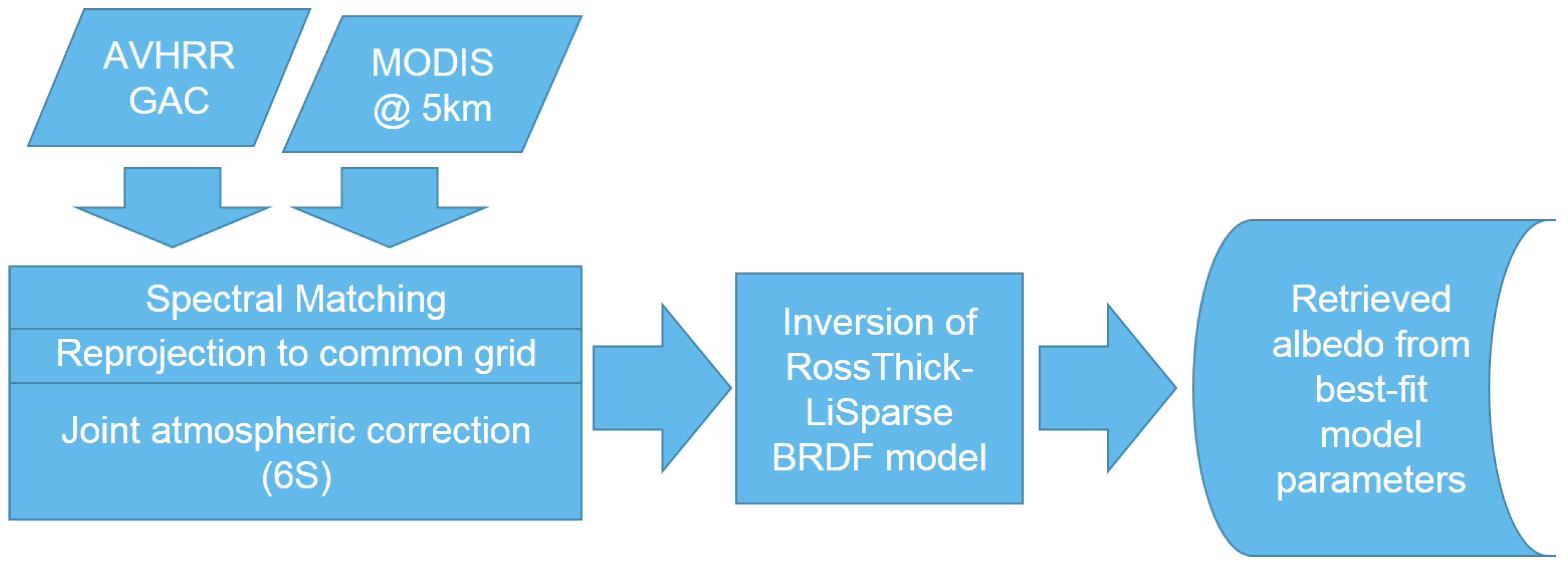
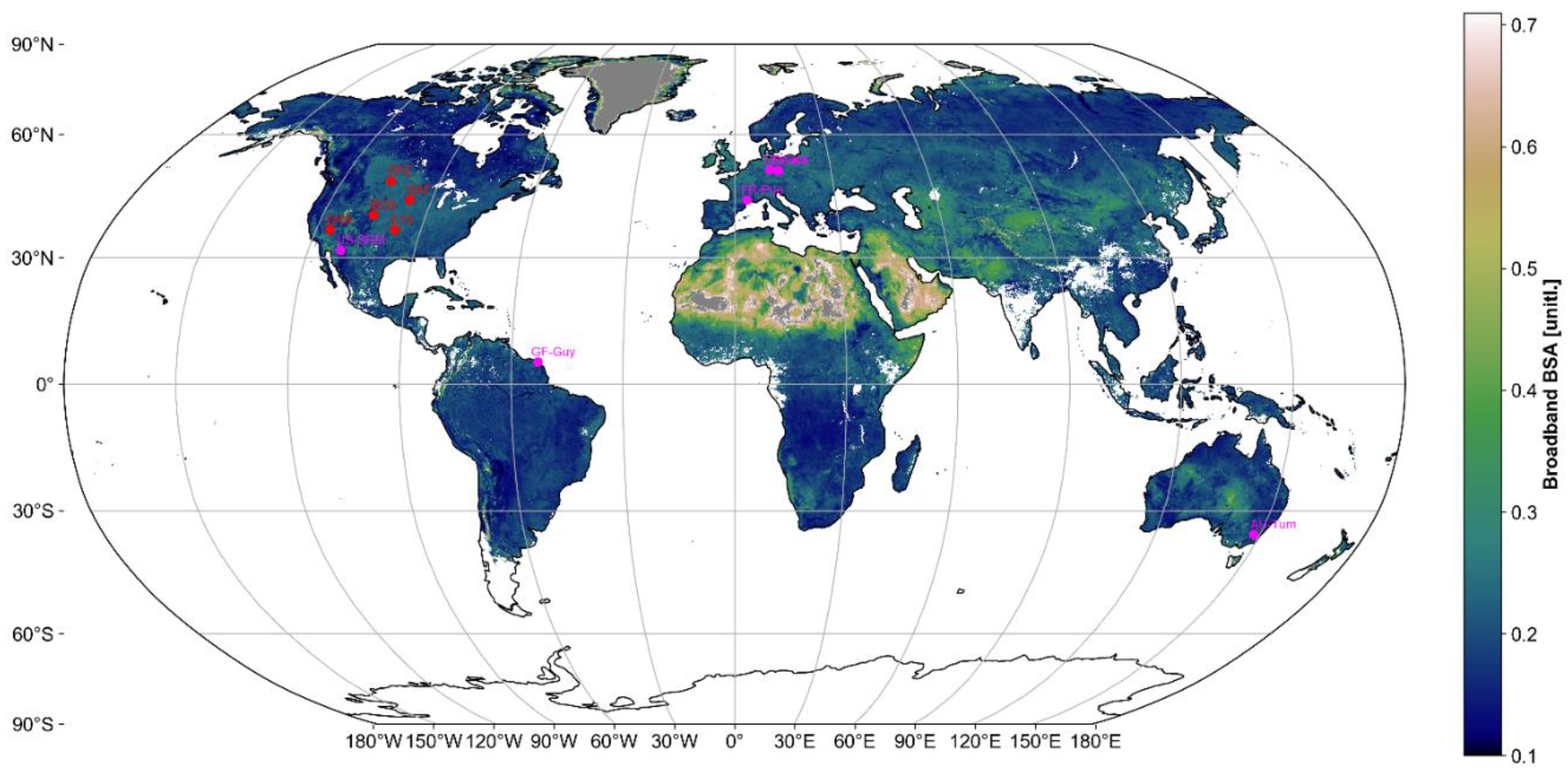
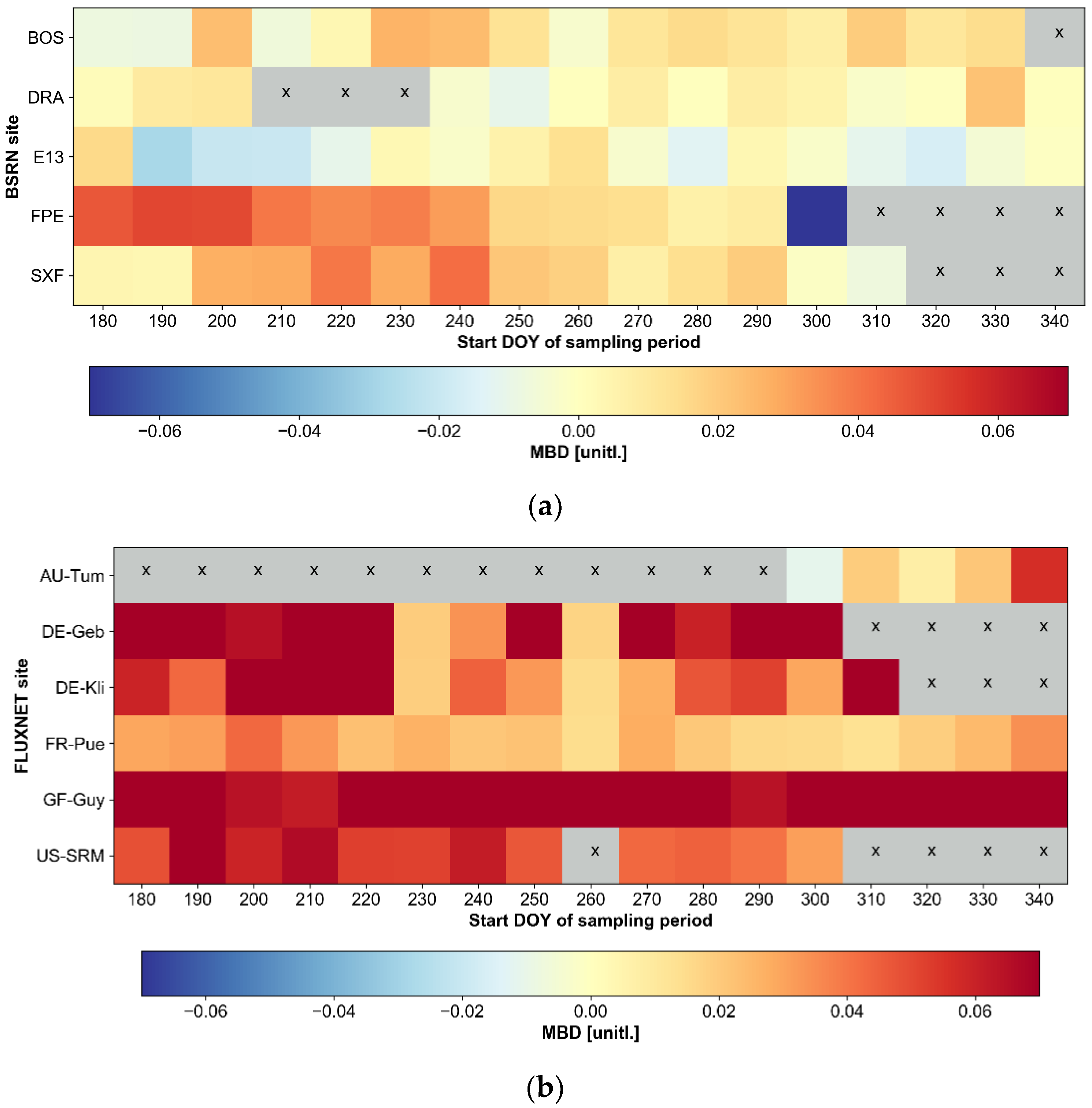
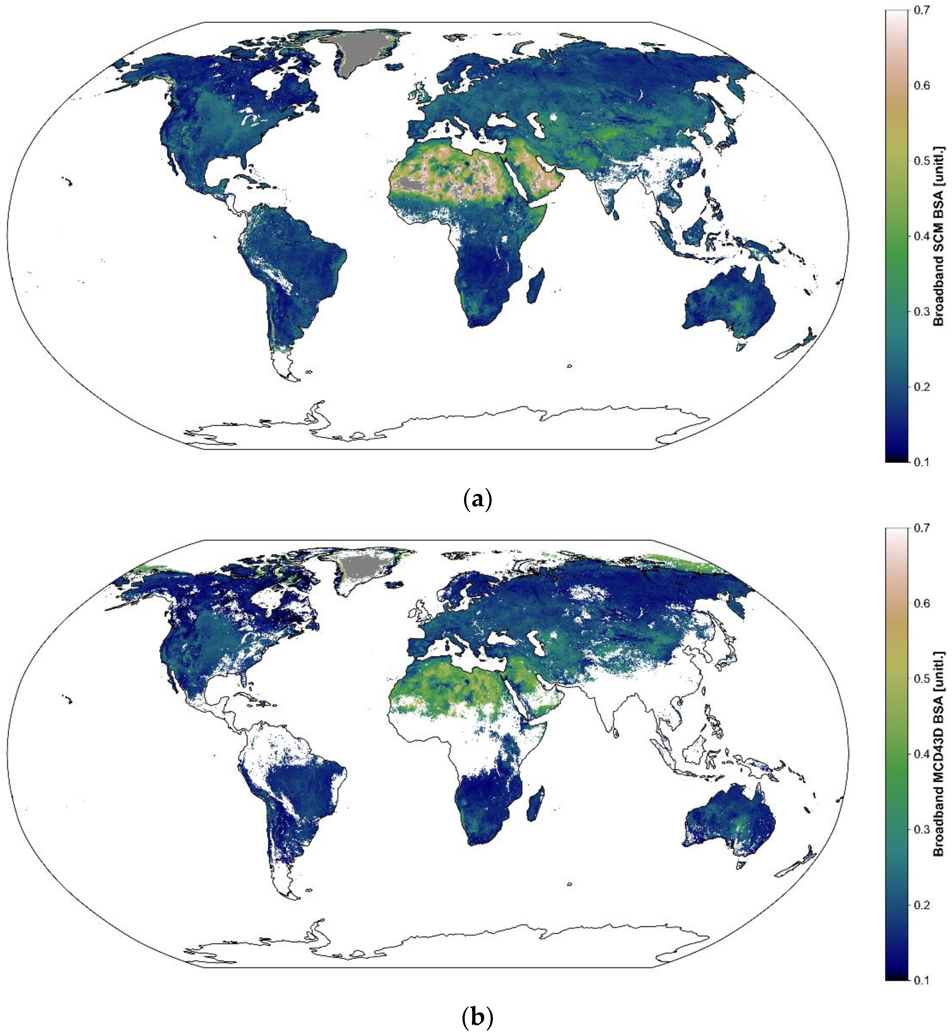
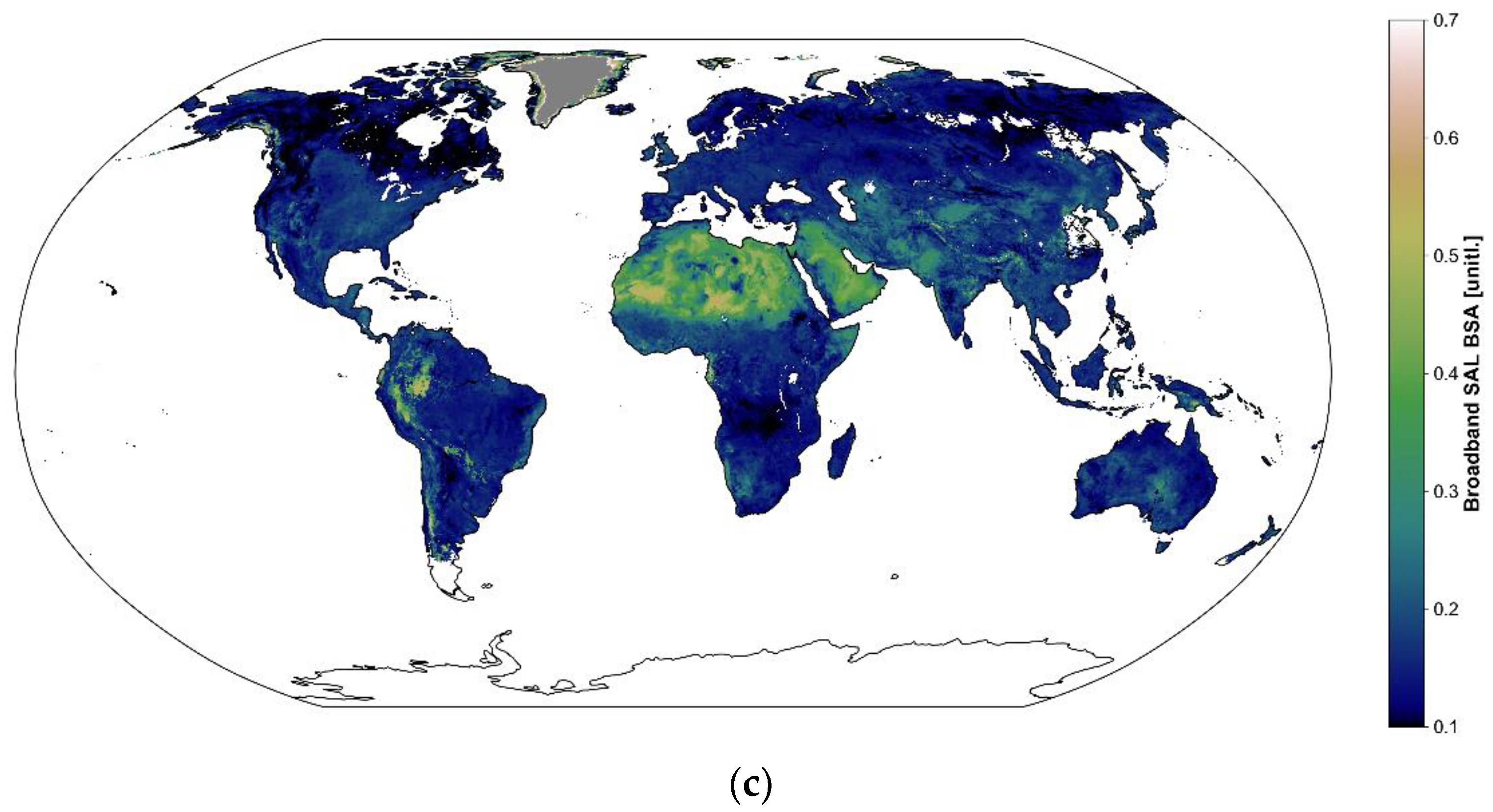
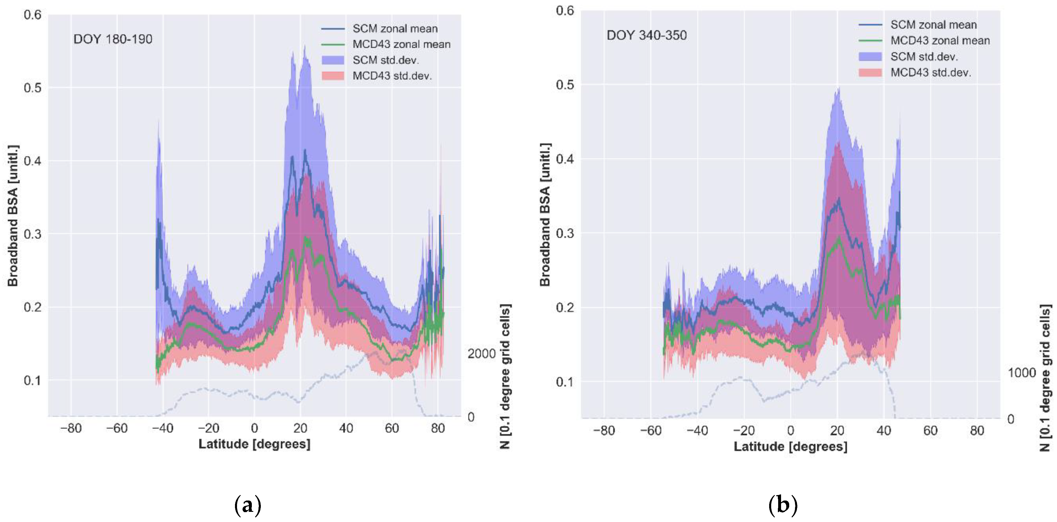
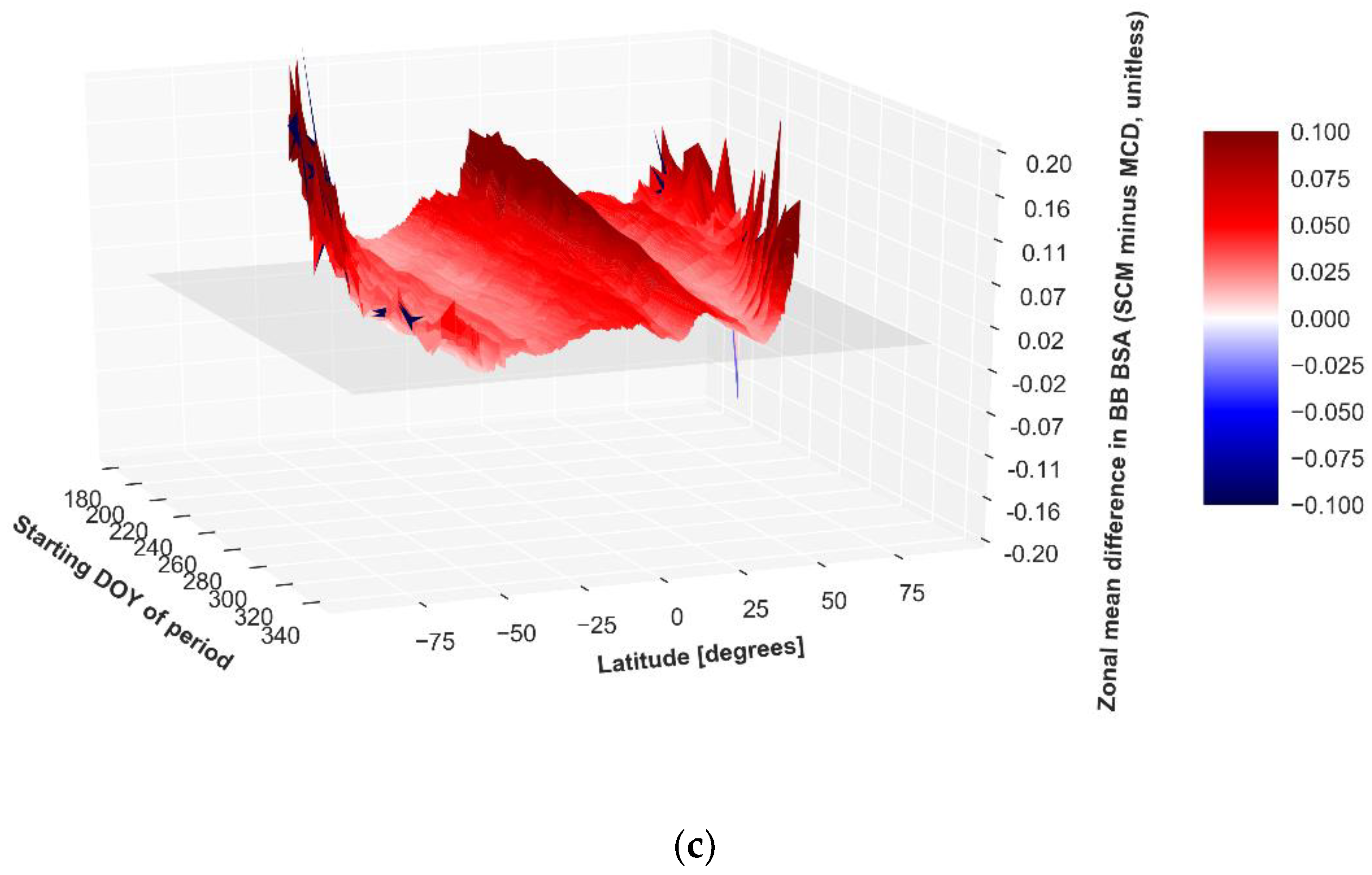
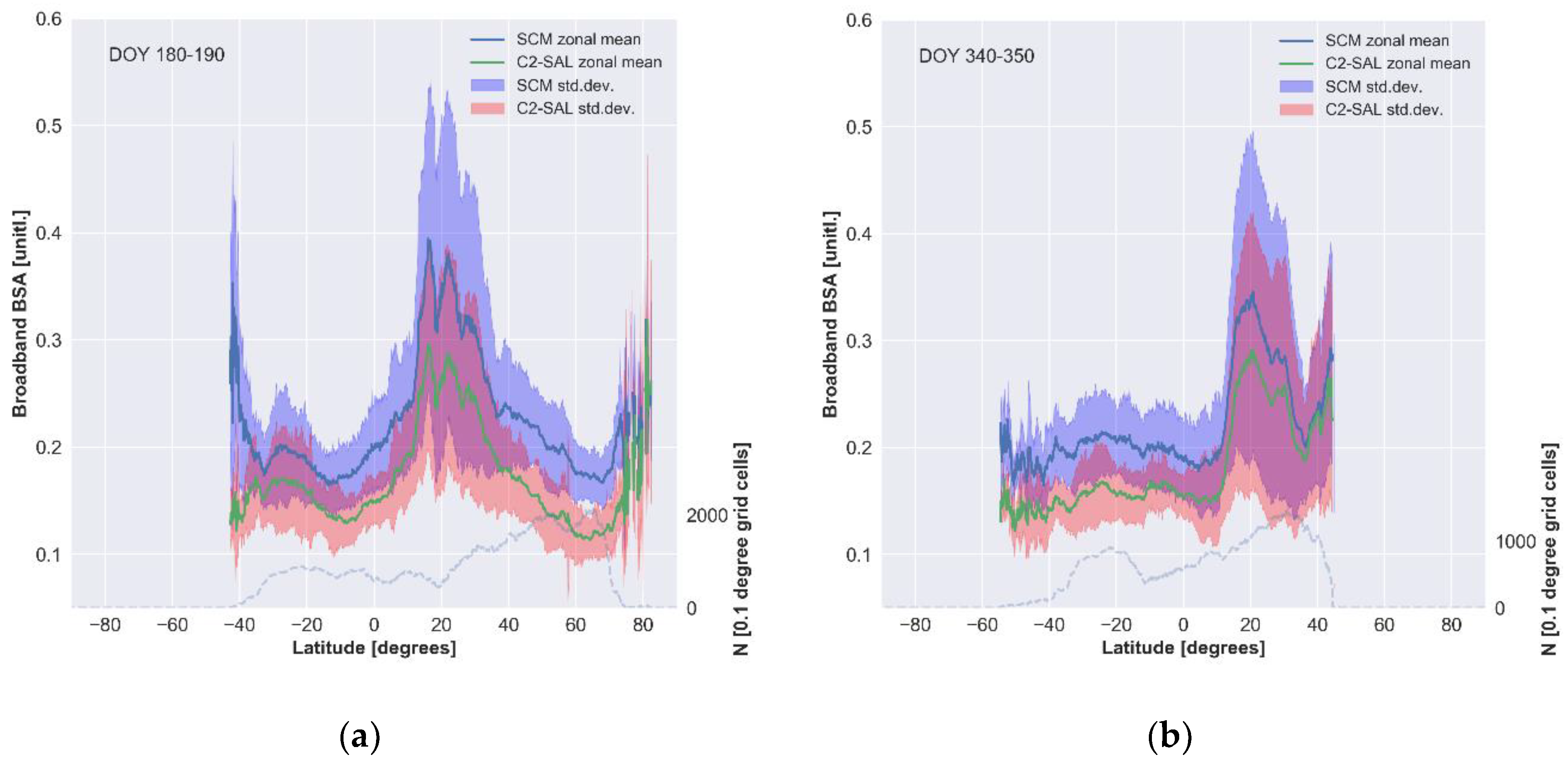
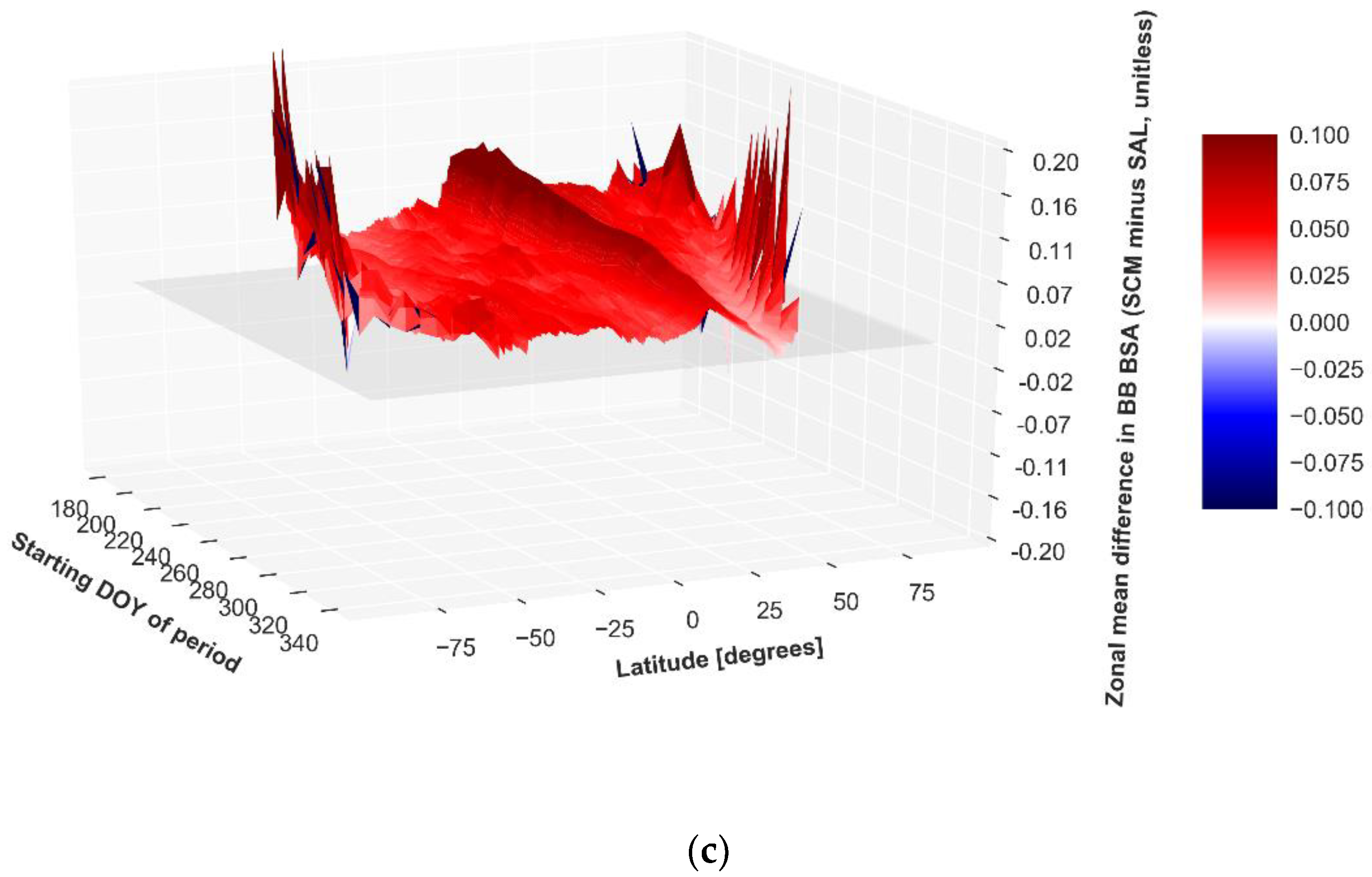
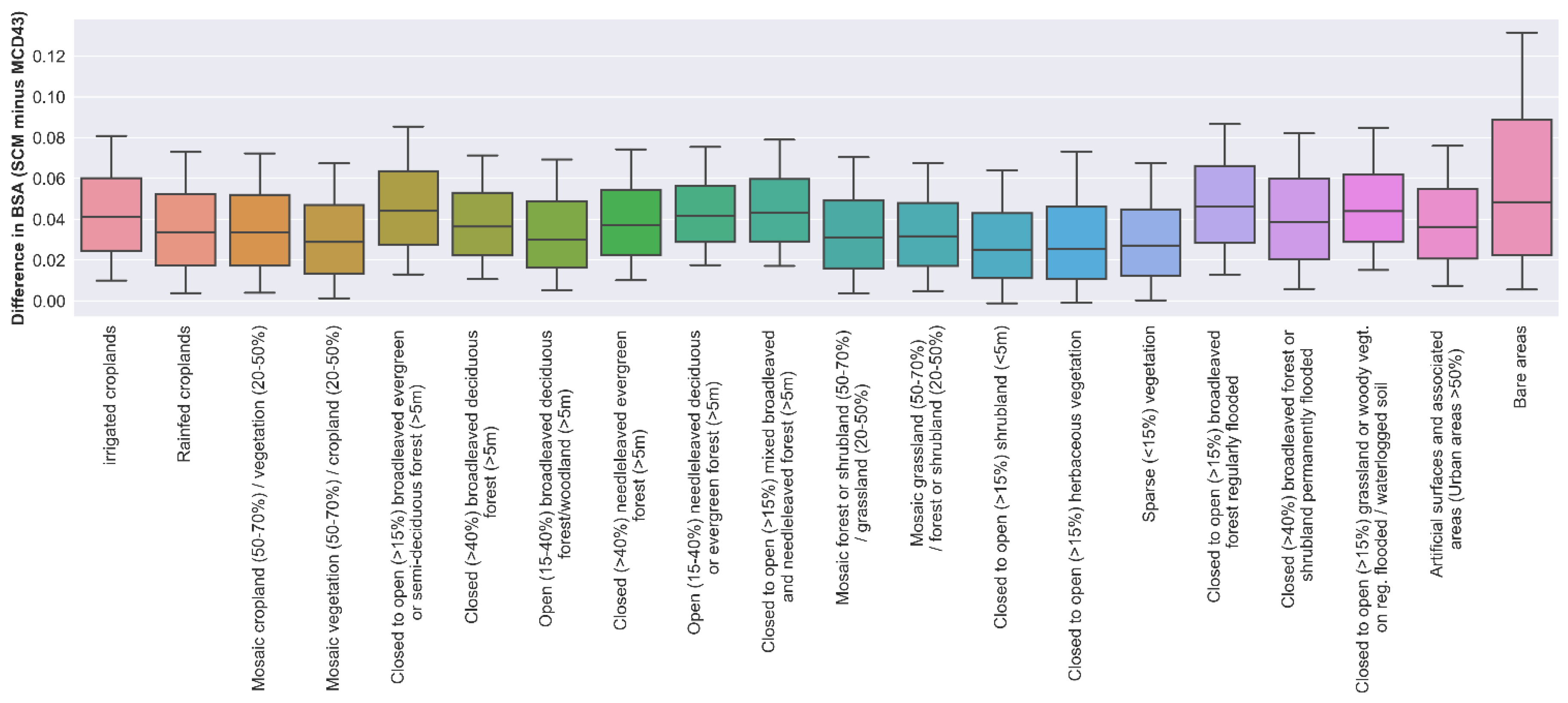
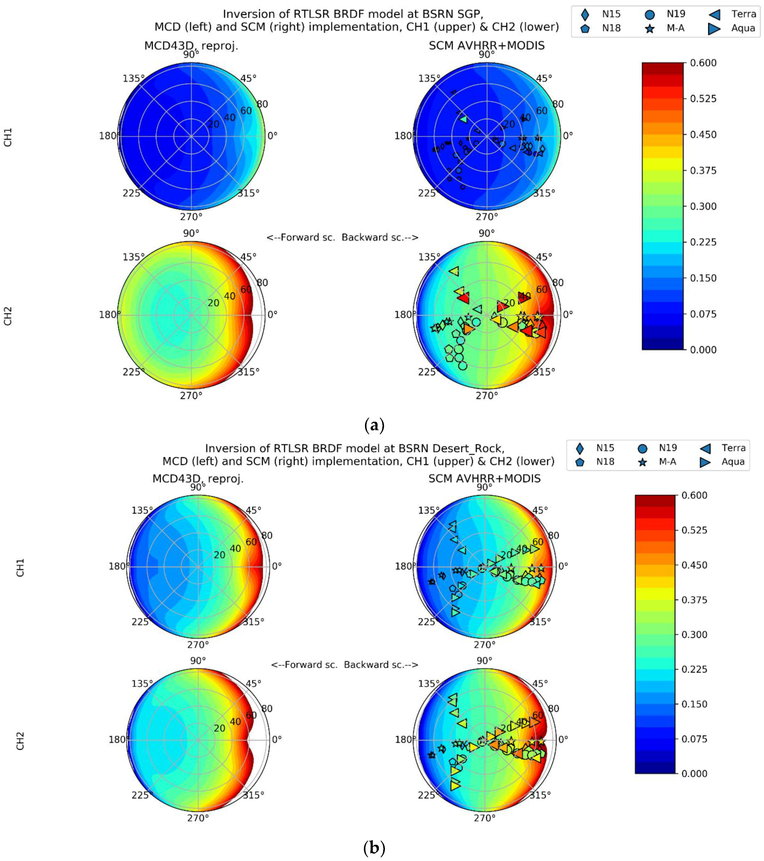
Table 1.
The dimensions and resolution for the 6S atmospheric correction LUT.
| Dimension | Start | Stop | Step | Unit | Data Source in Correction |
|---|---|---|---|---|---|
| Sun Zenith Angle (θs) | 0 | 70 | 10 | degree | Satellite orbital data |
| View Zenith Angle (θv) | 0 | 70 | 10 | degree | Satellite orbital data |
| Sun Azimuth Angle (φs) | 0 | 360 | 40 | degree | Satellite orbital data |
| View Azimuth Angle (φv) | 0 | 360 | 40 | degree | Satellite orbital data |
| Aerosol Optical Depth (AOD) | 0 | 1.5 | 0.1 | none | Aerosol CCI, monthly mean, v4.21 |
| Total water vapour column (H2O) | 0 | 6 | 0.5 | g/cm2 | CM SAF ATOVS, monthly mean, v1 |
Table 2.
The numeric g coefficients for Bidirectional Reflectance Distribution Function (BRDF) inversion from Reference [23]. The rows and columns here combine to form the various terms in Equations (4) and (5), for example, the first column and row represent the g0ISO term.
Table 2.
The numeric g coefficients for Bidirectional Reflectance Distribution Function (BRDF) inversion from Reference [23]. The rows and columns here combine to form the various terms in Equations (4) and (5), for example, the first column and row represent the g0ISO term.
| Term | Isotropic | Volumetric (RossThick) | Geometric (LiSparse-R) |
|---|---|---|---|
| g0 | 1.0 | −0.007574 | −1.284909 |
| g1 | 0.0 | −0.070987 | −0.166314 |
| g2 | 0.0 | 0.307588 | 0.041840 |
| White-sky g | 1.0 | 0.189184 | −1.377622 |
Table 3.
The BSRN and FLUXNET evaluation sites of this study.
| Site | Code | Latitude [°N] | Longitude [°E] | Surface Type/Topography |
| Boulder (SURFRAD) | BOS | 40.125 | −105.237 | Grass/flat |
| Desert Rock | DRA | 36.626 | −116.018 | Desert, gravel/flat |
| Southern Great Plains | E13 | 36.605 | −97.485 | Grass/flat |
| Fort Peck | FPE | 48.317 | −105.100 | Grass/flat |
| Sioux Falls | SXF | 43.730 | −96.620 | Grass/hilly |
| FLUXNET Sites | ||||
| Tumbarumba | AU-Tum | −35.657 | 148.902 | Evergreen broadleaf forest |
| Gebesee | DE-Geb | 51.100 | 11.664 | Cropland |
| Klingenberg | DE-Kli | 50.893 | 14.272 | Cropland |
| Puechabon | FR-Pue | 43.741 | 4.346 | Evergreen broadleaf forest, hilly |
| French Guiana | GF-Guy | 5.279 | −52.175 | Evergreen broadleaf forest (rain forest) |
| Santa Rita Mesquite | US-SRM | 31.821 | −110.116 | Shrubland |
Table 4.
The evaluation metrics for the BSRN and FLUXNET sites.
| BSRN Site | MBD | MABD | RMSD | Evaluated 10-Day Periods |
| Boulder (SURFRAD) | 0.010 | 0.013 | 0.015 | 16 |
| Desert Rock | 0.003 | 0.006 | 0.008 | 14 |
| Southern Great Plain | −0.005 | 0.010 | 0.013 | 17 |
| Fort Peck | 0.012 | 0.043 | 0.064 | 13 |
| Sioux Falls | 0.017 | 0.019 | 0.023 | 14 |
| FLUXNET Site | MBD | MABD | RMSD | |
| Tumbarumba | 0.018 | 0.023 | 0.029 | 5 |
| Gebesee | 0.074 | 0.074 | 0.083 | 13 |
| Klingenberg | 0.062 | 0.062 | 0.075 | 14 |
| Puechabon | 0.024 | 0.024 | 0.026 | 17 |
| French Guiana | 0.082 | 0.082 | 0.082 | 17 |
| Santa Rita Mesquite | 0.052 | 0.052 | 0.054 | 12 |
| Mean of sites | 0.032 | 0.037 | 0.043 | - |
© 2018 by the authors. Licensee MDPI, Basel, Switzerland. This article is an open access article distributed under the terms and conditions of the Creative Commons Attribution (CC BY) license (http://creativecommons.org/licenses/by/4.0/).
Share and Cite
MDPI and ACS Style
Riihelä, A.; Manninen, T.; Key, J.; Sun, Q.; Sütterlin, M.; Lattanzio, A.; Schaaf, C. A Multisensor Approach to Global Retrievals of Land Surface Albedo. Remote Sens. 2018, 10, 848. https://doi.org/10.3390/rs10060848
AMA Style
Riihelä A, Manninen T, Key J, Sun Q, Sütterlin M, Lattanzio A, Schaaf C. A Multisensor Approach to Global Retrievals of Land Surface Albedo. Remote Sensing. 2018; 10(6):848. https://doi.org/10.3390/rs10060848
Chicago/Turabian StyleRiihelä, Aku, Terhikki Manninen, Jeffrey Key, Qingsong Sun, Melanie Sütterlin, Alessio Lattanzio, and Crystal Schaaf. 2018. "A Multisensor Approach to Global Retrievals of Land Surface Albedo" Remote Sensing 10, no. 6: 848. https://doi.org/10.3390/rs10060848
Note that from the first issue of 2016, this journal uses article numbers instead of page numbers. See further details here.