Hydrologic Evaluation of Multi-Source Satellite Precipitation Products for the Upper Huaihe River Basin, China
by
 ,
,
Zhiyong Wu
1,2,* ,
,
Zhengguang Xu
1,2,
Fang Wang
3,
Hai He
1,2,
Jianhong Zhou
1,2,
Xiaotao Wu
1,2 and
Zhenchen Liu
1,2 1
Institute of Water Problems, Hohai University, 1 Xikang Road, Nanjing 210098, China
2
College of Hydrology and Water Resources, Hohai University, 1 Xikang Road, Nanjing 210098, China
3
Editorial Department of Journal, Hohai University, 1 Xikang Road, Nanjing 210098, China
*
Author to whom correspondence should be addressed.
Remote Sens. 2018, 10(6), 840; https://doi.org/10.3390/rs10060840
Submission received: 16 April 2018
/
Revised: 22 May 2018
/
Accepted: 24 May 2018
/
Published: 28 May 2018
(This article belongs to the Special Issue Remote Sensing of Precipitation)
Abstract
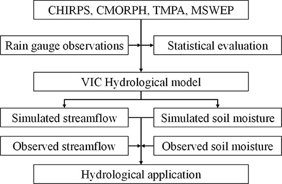
:To evaluate the performance and hydrological utility of merged precipitation products at the current technical level of integration, a newly developed merged precipitation product, Multi-Source Weighted-Ensemble Precipitation (MSWEP) Version 2.1 was evaluated in this study based on rain gauge observations and the Variable Infiltration Capacity (VIC) model for the upper Huaihe River Basin, China. For comparison, three satellite-based precipitation products (SPPs), including Climate Hazards Group InfraRed Precipitation with Station data (CHIRPS) Version 2.0, Climate Prediction Center MORPHing technique (CMORPH) bias-corrected product Version 1.0, and Tropical Rainfall Measuring Mission (TRMM) Multi-satellite Precipitation Analysis (TMPA) 3B42 Version 7, were evaluated. The error analysis against rain gauge observations reveals that the merged precipitation MSWEP performs best, followed by TMPA and CMORPH, which in turn outperform CHIRPS. Generally, the contribution of the random error in all four quantitative precipitation estimates (QPEs) is larger than the systematic error. Additionally, QPEs show large uncertainty in the mountainous regions, with larger systematic errors, and tend to underestimate the precipitation. Under two parameterization scenarios, the MSWEP provides the best streamflow simulation results and TMPA forced simulation ranks second. Unfortunately, the CHIRPS and CMORPH forced simulations produce unsatisfactory results. The relative error (RE) of QPEs is the main factor affecting the RE of simulated streamflow, especially for the results of Scenario I (model parameters calibrated by rain gauge observations). However, its influence on the simulated streamflow can be greatly reduced by recalibration of the parameters using the corresponding QPEs (Scenario II). All QPEs forced simulations underestimate the streamflow with exceedance probabilities below 5.0%, while they overestimate the streamflow with exceedance probabilities above 30.0%. The results of the soil moisture simulation indicate that the influence of the precipitation input on the RE of the simulated soil moisture is insignificant. However, the dynamic variation of soil moisture, simulated by precipitation with higher precision, is more consistent with the measured results. The simulation results at a depth of 0–10 cm are more sensitive to the accuracy of precipitation estimates than that for depths of 0–40 cm. In summary, there are notable advantages of MSWEP and TMPA with respect to hydrological applicability compared with CHIRPS and CMORPH. The MSWEP has a greater potential for basin–scale hydrological modeling than TMPA.
1. Introduction
Precipitation is an important component of the hydrological cycle and the most primary forcing data of hydrological models [1,2,3]. Accurate and reliable precipitation records are crucial, not only to investigate the spatial pattern and temporal change of precipitation but also to improve the accuracy of hydrological simulation [4,5].
Conventional rain gauge stations provide the most accurate point–based precipitation data. However, due to the high spatial heterogeneity of precipitation, it is inadequate to capture the spatial-temporal variability of precipitation systems based on unevenly and sparsely distributed rain gauge stations and hardly meets the needs of hydrological models and other related research [6,7]. A number of satellite-based precipitation products (SPPs) became available to the public such as the Climate Hazards Group Infrared Precipitation with Station data (CHIRPS) [8], Climate Prediction Center (CPC) MORPHing technique bias-corrected product (CMORPH CRT) [9], and Tropical Rainfall Measuring Mission (TRMM) Multi-satellite Precipitation Analysis (TMPA) 3B42 [10]. More recently, a lot of finer and more accurate SPPs have been released, such as Global Satellite Mapping of Precipitation (GSMaP) version 6 product [11] and Integrated Multi-satellite Retrievals for Global Precipitation Measurement (GPM) (IMERG) product [12]. A few preliminary assessments of GSMaP and IMERG suggest a great potential for the hydrological applications [13,14,15,16]. The SPPs have a wide spatial coverage and high spatiotemporal resolution, effectively making up deficiencies of the conventional rain gauge observations and greatly enriching alternative precipitation data sources, especially in data-scarce or ungauged regions [17,18]. Benefitting from these advantages, the SPPs have been extensively applied in many fields such as hydrological simulations [2,14,17,19], extreme events analysis [20,21,22,23], and water resource management [24]. However, the SPPs are inevitably subject to errors resulting from sampling uncertainties and retrieval algorithms; furthermore, the error characteristics change depending on the climate regions, seasons, altitudes, and other factors [3,7,25,26].
To minimize the limitations of individual precipitation products, many researchers focused on merging different precipitation datasets to obtain a higher-quality gridded precipitation product [27,28,29,30,31]. Recently, the global gridded precipitation dataset Multi-Source Weighted-Ensemble Precipitation (MSWEP) that optimally merges gauge, satellite, and reanalysis data has been produced by Beck et al. [1,28]. The latest version MSWEP V2.1 with 3-hourly temporal and 0.1° spatial resolution has been available to the public since 20 November 2017. Tong et al. [32] pointed out that the SPPs are most accurate during summer and at lower latitudes, while atmospheric model reanalysis datasets perform better than SPPs during winter and at higher latitudes. Therefore, the MSWEP V2.1 can take full advantage of the complementary nature of satellite and reanalysis data and offers the prospect of increasing the precision of precipitation estimates. Due to its high spatial resolution, long time span, and great potential for hydrological applications, the MSWEP V2.1 has received the wide attention of hydrologists since its release. The research on the applicability and efficiency of MSWEP V2.1 in hydrological simulations is in progress. To evaluate the error characteristics of merged precipitation products and their performance in hydrological simulations at the current technical level of integration, the MSWEP V2.1 is used as a typical representative of merged precipitation products in this study and its applicability of MSWEP V2.1 is evaluated based on a typical semi-humid and semi-dry climatic transitional region of China.
Generally, the error characteristics of quantitative precipitation estimates (QPEs) can be directly quantified based on sufficient rain gauge observations. The direct evaluation for the error characteristics of QPEs is very important to improve the gauge adjustment scheme or merging procedure and can further be used to determine the impact of the error characteristics of QPEs on hydrological simulations. The quality of QPEs can impact the hydrologic outputs through the rainfall-runoff response [19]. Thus, the applicability analysis of QPEs in hydrological modeling serves as an alternative validation method and is more efficient than using limited rain gauge observations as a reference to better understand the properties and optimal hydrological usage of QPEs in data-scarce regions [2]. The applicability of QPEs to streamflow simulation has been evaluated in numerous studies. With the exception of streamflow, macroscale land surface hydrological models also provide an alternative way to reconstruct and continually update the spatial and temporal distribution of soil moisture over a large area [33]. Thus, indirect evaluation work can also be accomplished by evaluating the potential of QPEs in soil moisture simulation.
Based on these considerations, this study aims to statistically assess the MSWEP V2.1 against a relatively dense network of rain gauge stations and then evaluate its hydrological performance from multiple perspectives under two parameterization scenarios in the upper Huaihe River Basin. Subsequently, the impacts of QPE errors on the simulated streamflow and soil moisture are analyzed. For comparison, CHIRPS V2.0, CMORPH CRT V1.0, and TMPA 3B42 V7 are also evaluated in this study. The results provide a perspective on error characteristics and the hydrological applicability of the MSWEP V2.1 in regions with similar terrains and climates.
The rest of the paper is organized as follows: The study area and datasets used in this study are introduced in Section 2. The methodology, including the Variable Infiltration Capacity (VIC) hydrologic model and some evaluation metrics, is described in Section 3. The results of the statistical evaluation and hydrological simulation are presented in Section 4, followed by the discussion (Section 5) and main conclusions (Section 6).
2. Study Area and Data
2.1. Study Area
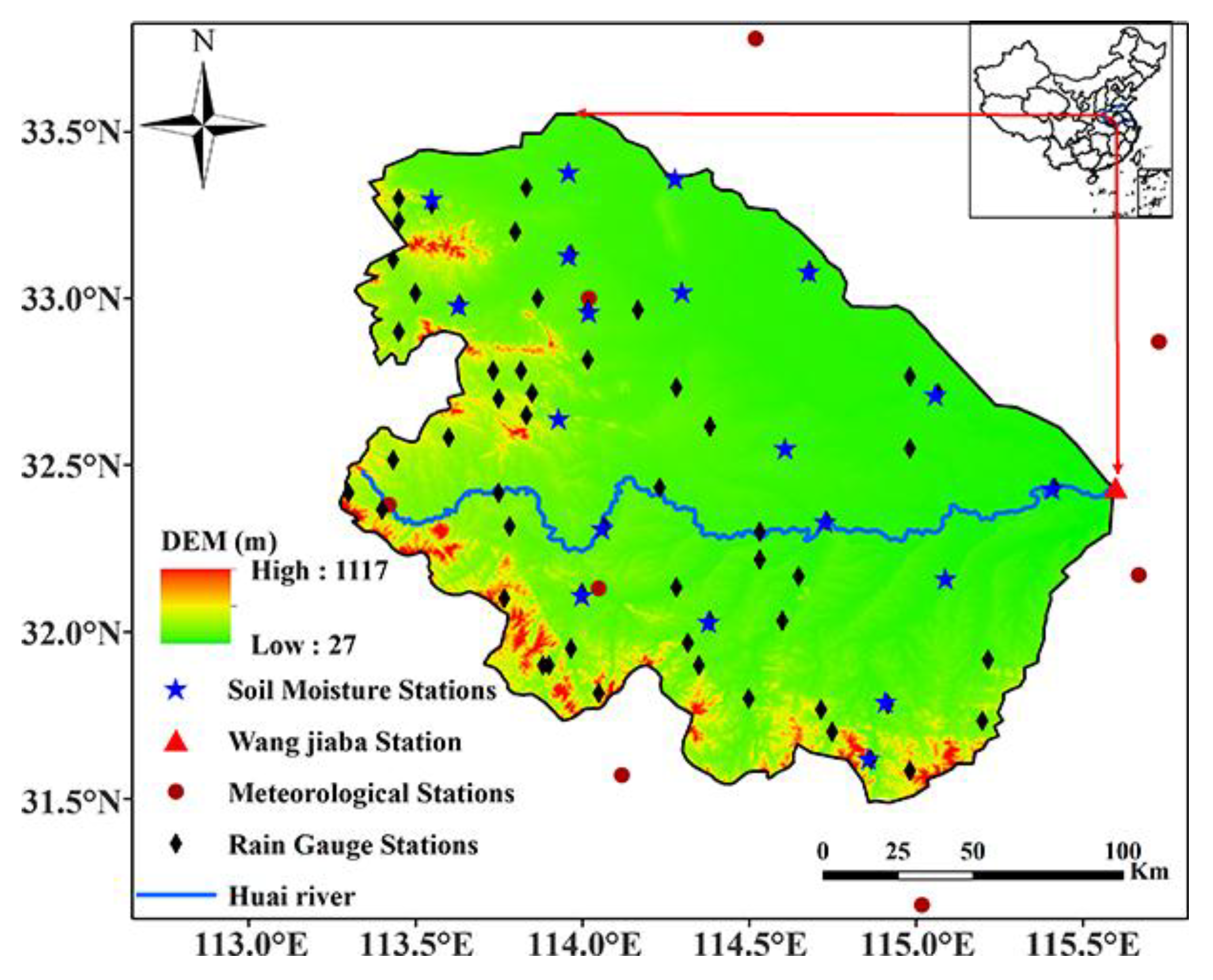
The Huaihe River Basin in eastern China has a drainage area of approximately 270,000 km²; it is also the line of demarcation between Chinese southern and northern climates. The Huaihe River Basin suffers from frequent drought and flood disasters due to the uneven spatiotemporal distribution of precipitation influenced by complex and changeable climate. The Wangjiaba Station in the main stream of the Huaihe River Basin plays a vital role in flood control and management [34]. The study area is the upper region of Wangjiaba Station in the Huaihe River Basin, which has a drainage area of 30,630 km². Its terrain gradually lowers from west to east (Figure 1). The flood season ranges from June to September.
2.2. Data
2.2.1. Precipitation
This study aims to assess the error characteristics of four QPE products and their hydrological application. A brief introduction to the four QPE products and rain gauge observations is provided in this section.
The CHIRPS is a quasi-global rainfall dataset, which was specially developed for drought monitoring. As of February 2015, version 2.0 of CHIRPS is complete and available to the public. Several data sources were introduced for the construction of CHIRPS product such as the monthly precipitation climatology CHPclim, infrared measurements from geostationary satellites, TMPA 3B42 product, and rain gauge data [8]. The daily CHIRPS V2.0 with a spatial resolution of 0.25° was selected for this study.
NOAA’s CPC CMORPH contains global satellite–based precipitation generated by integrated microwave data and infrared data [9]. The CMORPH combines the superior retrieval accuracy of passive microwave estimates and the higher temporal and spatial resolution of infrared data. The latest CMORPH V1.0 product includes CMORPH RAW, CMORPH CRT, and CMORPH BLD, covering 60°S–60°N, 180°W–180°E. The CMORPH CRT with 3 h temporal and 0.25° spatial resolutions were used in this study.
The TMPA products were designed based on a wide variety of satellite datasets and supplied by NASA [10]. The two latest version 7 products of the TMPA (quasi-near-real-time 3B42RT V7 and post-real-time 3B42 V7) are the most prevalent at present. The 3B42V7 product was adjusted by monthly rain gauge precipitation data from the Global Precipitation Climatology Center (GPCC) and is superior to the TMPA 3B42RT V7. The TMPA 3B42V7 with a spatiotemporal resolution of 3 h and 0.25° were used in this study.
The MSWEP version 2.1 is a new global historic precipitation dataset (1979–2016) with 3-hourly temporal and 0.1° spatial resolution, which was specially designed for hydrological modeling. The design philosophy of MSWEP was to optimally merge the highest quality precipitation data sources as a function of timescale and location, the temporal variability of MSWEP was determined by weighted averaging. For each grid cell, the weight varies according to the network density and the accuracy of satellite- and reanalysis-based estimates [28].
The daily precipitation data of 57 rain gauges from 2000 to 2010 provided by the Hydrology Bureau of the Huaihe Water Conservancy Commission were used to evaluate the four QPEs mentioned above. For convenience, the precipitation datasets used in this study are given short names, as described in Table 1.
In this study, the VIC model is run at a spatial resolution of 0.05° × 0.05° using a daily time step. This means that, before starting the evaluation, all four QPEs and rain gauge observations are aggregated into a 0.05° × 0.05° spatial grid using the bilinear interpolation and the inverse distance weighted method, respectively. The precipitation products with 3 h temporal resolution are integrated over time to daily accumulated values.
2.2.2. Streamflow and Soil Moisture
Daily streamflow records of the Wangjiaba Station were derived from hydrologic year books published by the Hydrologic Bureau of the Ministry of Water Resources of China.
The observed soil moisture data were downloaded from the Ministry of Water Resources of China. The soil moisture has been routinely measured at three different depths (10, 20, and 40 cm) three times per month, on the 1st, 11th, and 21st, since 2008 using the oven–drying method. A total of 19 soil moisture observation stations are located in the study area (Figure 1). To maintain consistency with the model simulated soil moisture, gravimetric soil moisture data at a depth of 0–10 cm and 0–40 cm were translated to volumetric soil moisture data using the soil bulk density of each 0.05° grid.
3. Methodology
3.1. VIC Hydrological Model and Calibration Methods
The VIC grid-based macroscale semi-distributed hydrological model was developed by Liang et al. [35]. The VIC model uses a spatial probability distribution function to represent the subgrid variability of the soil moisture storage capacity, which more realistically treats the hydrological processes within a model grid cell [33]. In this study, the VIC model was applied on each grid point for the calculation of the water balance using a daily time step. The observed daily maximum and minimum air temperature data from 2000 to 2010 required for the VIC model were derived from eight meteorological stations within and around the upper Huaihe River Basin provided by the China Meteorological Data Sharing Service System. For each grid, the global 1 km land cover classification dataset [36] and the global 10 km soil types dataset [37] were used to define the vegetation and soil parameters. The geographical parameters were calculated using meteorological variables and the location of the study region.
The hydrological parameters of the VIC model are closely related to the runoff yielding process and are difficult to directly determine, thus, it should be calibrated using observed hydrographs. These parameters include the exponent of variable infiltration capacity curve (B), the maximum velocity of the base flow (Dsmax), the fraction of Dsmax where non-linear base flow begins (Ds), the fraction of maximum soil moisture when non-linear base flow occurs (Ws), and the depth of the second and third soil layer (d2 and d3, the thickness of the first soil moisture layer being fixed at 0.1 m). Based on the method that integrated the Rosenbrock algorithm [38] and manual intervention, the hydrological parameters were optimized and determined. The manual intervention is to determine the initial values and a reasonable range of the parameters according to the physical meaning of the parameters and the characteristics of the basin. Then the hydrological parameters were automatically calibrated using the Rosenbrock algorithm by maximizing the Nash-Sutcliffe coefficient of Efficiency (NSCE) and simultaneously minimizing the relative error (RE) between observed and simulated streamflow.
The hydrological simulation was conducted under two parameterization scenarios to evaluate the hydrological application of the four QPEs. In Scenario I, the VIC model calibration and validation were forced by the HWCC to obtain optimal hydrological parameters. The four QPEs were then used as forcing data to simulate the streamflow and soil moisture. Scenario I was mainly used to directly compare the influence of different precipitation products on the accuracy of the hydrological simulation. In Scenario II, all these hydrological parameters were recalibrated separately using the precipitation from CMORPH, CHIRPS, TMPA, and MSWEP. Subsequently, the hydrological simulation was conducted using both parameters recalibrated under scenario II and the corresponding precipitation estimate. Scenario II can be used to determine if the evaluated precipitation products have the potential to be alternative data sources for hydrological simulations in data–poor or ungauged basins [14,19].
Considering that the study area was dominated by the low-flow years after 2008, 2005–2010 and 2002–2004 were selected as the calibration and validation periods in both scenarios, respectively, to balance the high-flow years and low-flow years and prevent overfitting during high-flow years. To eliminate the influence of the initial state on the simulation results, the VIC model was prerun for two additional years before the calibration and validation period to initiate the model state in both scenarios.
3.2. Evaluation Metrics
Several verification indices were used to quantitatively assess the error characteristics of the QPE, including the relative error (RE), root mean square error (RMSE), and correlation coefficient (CC). The mean square error (square of RMSE, MSE) is composed of the systematic error (MSEsys) and random error (MSEran) [4]; thus, two error components were assessed for each QPE in this study. In addition, the frequency bias (FBI), the probability of detection (POD), the false alarm ratio (FAR), and the equitable threat score (ETS) were calculated to quantitatively evaluate the accuracy of the four QPEs under different precipitation thresholds.
Specifically, the NSCE and exceedance probabilities (Pm) were added to the RE to evaluate the simulated discharge. The simulated soil moisture was assessed based on several metrics including the RE, CC, and unbiased root mean square error (ubRMSE). The ubRMSE removes the bias from the RMSE and can reasonably reflect the random error of the simulated soil moisture [39]. The equations to calculate the above-mentioned indices are listed in Table 2.
4. Results
4.1. Evaluation and Comparison of Different Precipitation Products
4.1.1. Spatiotemporal Characteristics
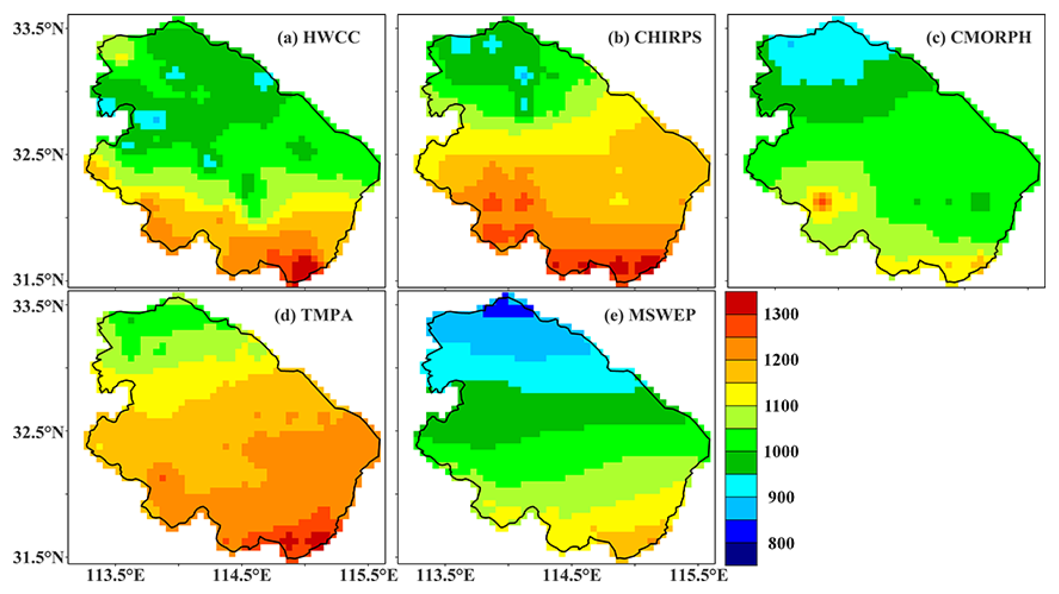
Figure 2 presents the spatial distribution of the average annual precipitation of the HWCC and four QPEs during 2000 and 2010. All four QPEs generally show a consistent spatial pattern with the precipitation decreasing from south to north, which agrees with the HWCC.
The spatial distribution and seasonal variability of the RE, RMSE, and CC of the four QPEs are listed in Figure 3 and Table 3. Based on the RE for the whole study period (Figure 3a1–a4), CHIRPS and TMPA generally overestimate the precipitation with a grid–averaged RE of 7.1% and 10.4%, respectively. However, the RE of the CHIRPS and TMPA in the northwestern and southern mountain areas (less than 6% or underestimate) are significantly lower than the RE in the central parts of the basin. The similar error features of CHIRPS and TMPA may be attributed to the use of the TMPA for the generation of CHIRPS [8,40]. Conversely, CMORPH and MSWEP are dominated by an overall negative RE, especially in the northwestern and southern parts of the basin; the grid–averaged RE of CMORPH and MSWEP are −3.3% and −5.4%, respectively. The significant difference in the RE between TMPA and CMORPH is consistent with the results of Sun et al. [19], which might partly be due to the difference in the retrieval algorithms. With respect to seasonal variations (Table 3), negative REs of CMORPH and MSWEP are significant in spring and winter and the TMPA shows a considerable overestimation in winter, which can be attributed to the low amount of precipitation in these two seasons and the weak detection to the snow and light rainfall events of the satellite sensors [13,14]. The CHIRPS shows a consistent overestimation, especially in summer with more intense precipitation than in other seasons, which is similar to the results of Duan et al. [41].
The differences of the RMSE (Figure 3b1–b4) and CC (Figure 3c1–c4) for different QPEs are significant; however, the spatial distributions of CC and RMSE for a specific precipitation product are homogeneous. Throughout the whole period, the MSWEP is superior to the other three QPEs, with the lowest RMSE (≤6 mm/day in nine out of ten of the study areas) and the highest CC (almost all above 0.8), which may be due to the use of the reanalysis datasets in MSWEP, providing a unique advantage over other QPEs [42]. The performances of CMORPH and TMPA are very similar, with the RMSE ranging from 5.0 to 8.0 mm/day and CC varying from 0.7 to 0.8 in most parts of the basin, which may be due to the similar data sources used in these two QPEs [9,10]. The CHIRPS exhibits the worst performance, with an RMSE above 7.0 mm/day and CC mainly between 0.6 and 0.7. The poor performance of CHIRPS may be attributed to cloud–top infrared (IR) observations [41]. As shown in Table 3, the RMSE and CC values generally demonstrate seasonal variations, except for the CC of MSWEP. All four QPEs have the smallest and largest RMSE values in spring and autumn. However, the QPEs perform poorly in spring in terms of CC, except for MSWEP. Additionally, the MSWEP is superior to the other three QPEs based on the CC and RMSE values in every season. In contrast, CHIRPS provides the worst estimates based on the RMSE and CC.
The contributions of systematic and random error components to the mean square error are presented in Figure 4. The spatial distribution of the systematic (random) error has a similar pattern for all QPEs. The random error component clearly dominates the four QPEs, which is due to the adjustment of all precipitation products by rain gauge observations. Mountainous regions exhibit larger systematic errors than plain areas, which can be attributed to the higher uncertainty of precipitation estimates in mountainous regions [4]. This shows that the existing methods of bias correction are not as effective at higher altitudes as at lower altitude areas and the integration of different precipitation products does not seem to be a solution to this problem. Therefore, the effect of the terrain should be further considered during bias correction or multi–source precipitation fusion.
All four QPEs tend to underestimate the precipitation in the northwestern and southern mountainous areas, which is probably caused by the higher temporal variability of precipitation in the mountainous regions. However, limited by the revisiting period of the satellite, satellite-based precipitation estimates are generally incapable of reflecting temporal variability well in mountainous precipitation. The standard deviation (SD) of grid-based daily precipitation can be used as a measure of temporal variability of daily precipitation, and the spatial distribution of the SD of the daily precipitation reflects the spatial heterogeneity of regional precipitation. The SD of each VIC grid was calculated based on the HWCC. Subsequently, the relationships between the REs of the four QPEs and SD were analyzed. As presented in Figure 5, there are remarkable negative correlations between the REs of the QPEs and SD (CC = −0.55, −0.62, −0.77, and −0.66 for CHIRPS, CMORPH, TMPA, and MSWEP, respectively), which indicate that the QPEs tend to underestimate the precipitation in regions with higher temporal variability of the daily precipitation and the spatial heterogeneity of daily precipitation will affect the spatial distribution of the RE of the QPEs.
4.1.2. Results for Different Rainfall Intensity
The accuracy of the four QPEs under different precipitation thresholds was evaluated based on four statistical scores (Figure 6). The results of the FBI are related to the RE of the QPEs. The analyzed precipitation with positive (negative) RE generally overestimates (underestimates) the occurrence of rain events across most thresholds. All four QPEs underestimate the occurrence of rain events when the daily precipitation is above 85.0 mm, especially the MSWEP. The overall precipitation accuracy of the four QPEs (based on POD, FAR, and ETS) declines with increasing precipitation threshold, indicating that the QPEs are less capable of depicting intense precipitation. As a whole, the MSWEP exhibits a more stable discrimination skill across all precipitation thresholds with the lowest FAR and highest POD and ETS. The TMPA shows slightly better skills than the CMORPH at most thresholds and CHIRPS performs the worst.
4.2. Evaluation of the Streamflow Simulation under Two Parameterization Scenarios
In this section, we evaluate and inter-compare the hydrological applicability of the four QPEs by performing a streamflow simulation using the VIC model under two parameterization scenarios.
4.2.1. Scenario I: Model Parameters Calibrated by Rain Gauge Observations
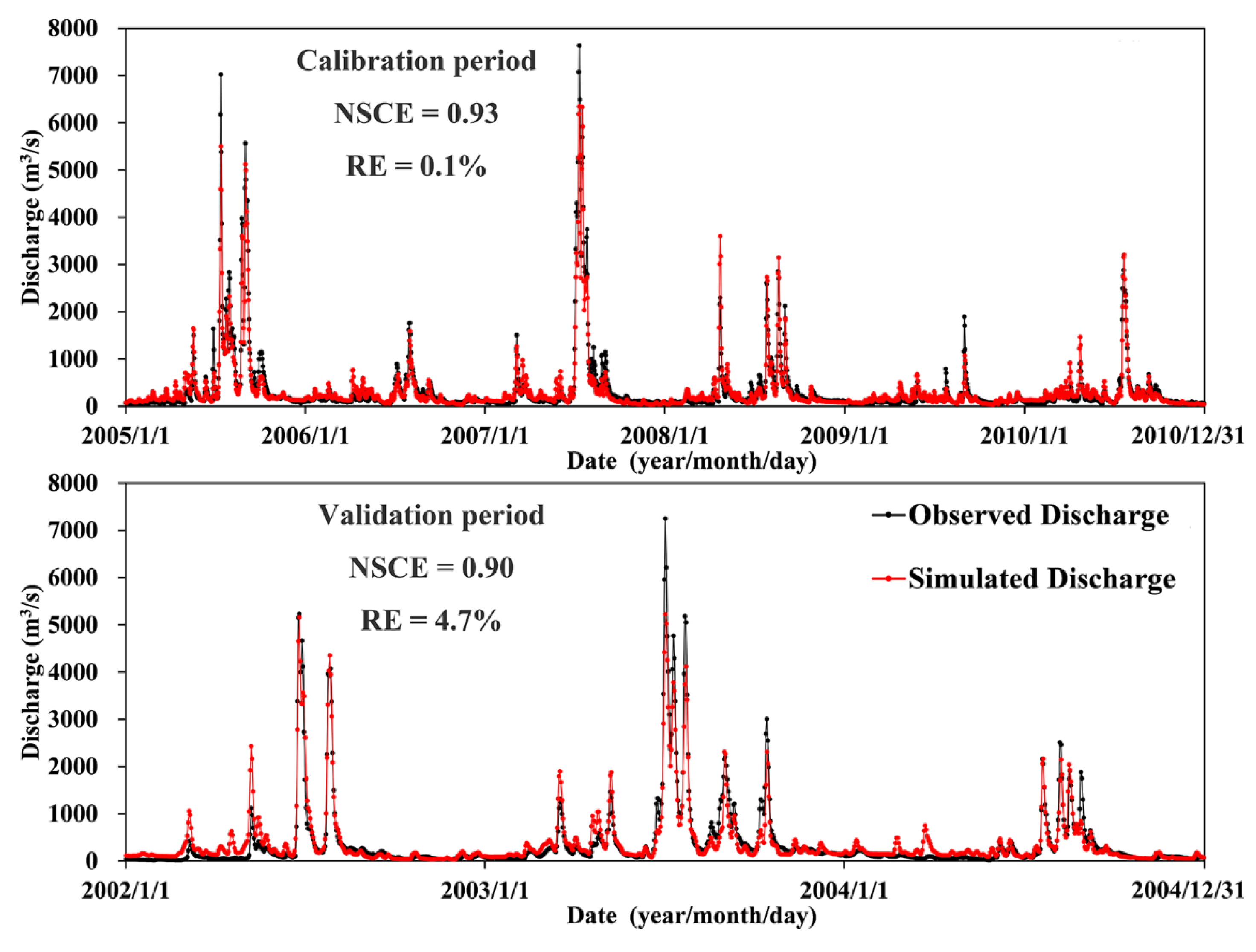
Figure 7 shows the observed and simulated streamflow driven by the HWCC for the calibration and validation period. Generally, the streamflow simulated by HWCC is in good agreement with the observed streamflow with high NSCE of 0.93 and almost no RE for the calibration period, and still maintains a high NSCE of 0.90 and small RE of 4.7% for the validation period. The simulated results indicate that the adaptability of the VIC model and model parameters calibrated by the HWCC are reasonable. Thus, it is suitable to evaluate the applicability of the four QPEs.
The VIC model was forced by four QPEs using the model parameters calibrated by the HWCC to simulate the streamflow from 2002 to 2010. As shown in Table 4, the CMORPH and MSWEP forced simulations underestimate the streamflow, while the CHIRPS and TMPA forced simulations overestimate the streamflow, which is related to the RE of the corresponding forcing data and indicates that the biases of the QPEs can directly propagate to streamflow simulations [7]. The MSWEP performs best in the streamflow simulation with the largest NSCE (0.87 and 0.74, respectively). The TMPA takes the second place in terms of NSCE (0.66 and 0.69, respectively), as well as with highest RE (30.8% and 19.1%, respectively). The CHIRPS generally performs poorly throughout the whole period. The simulated results of CMORPH for the calibration and validation period significantly differ, which indicates that the stability of CMORPH is poor.
4.2.2. Scenario II: Model Parameters Separately Recalibrated Using the QPEs
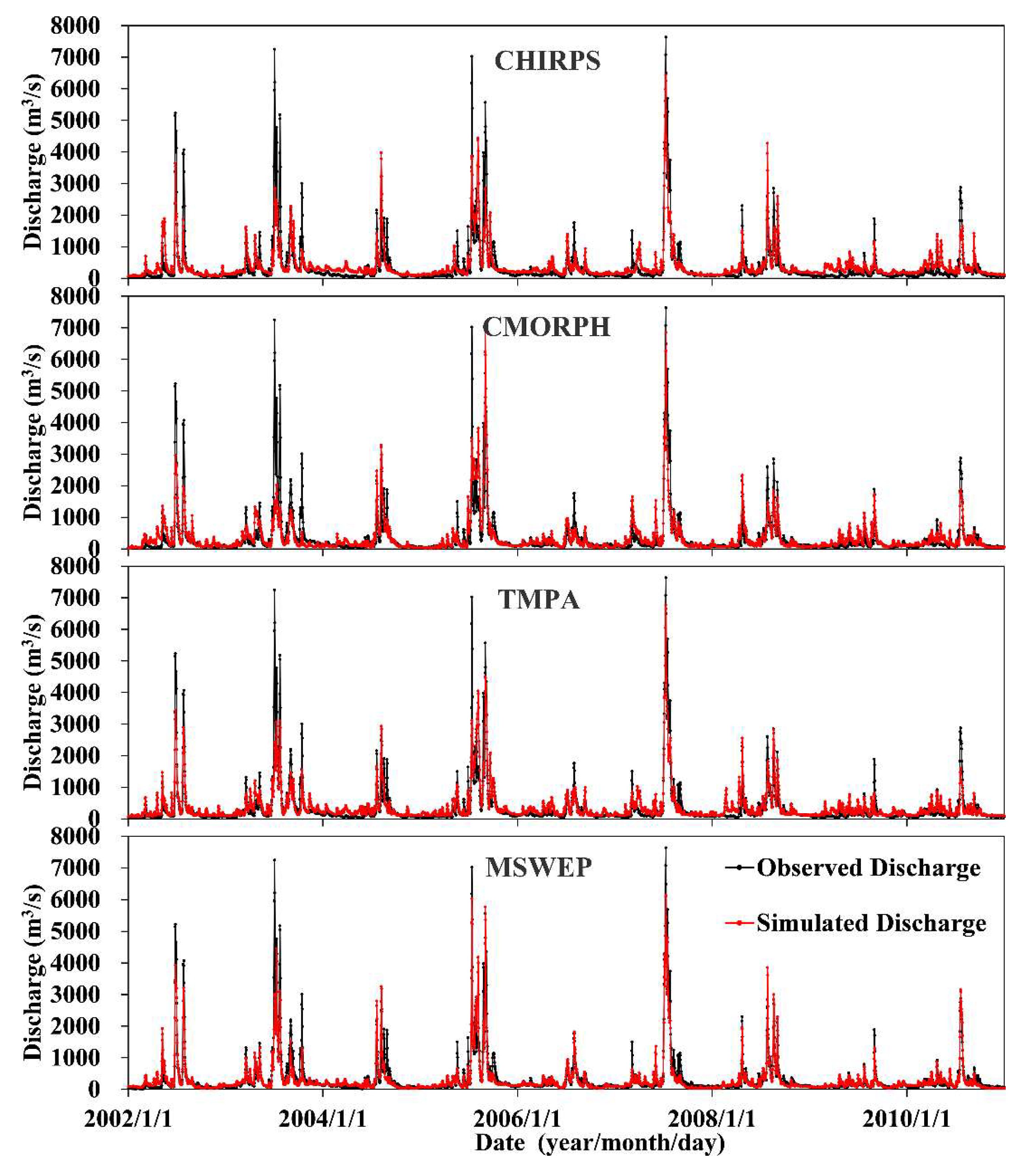
The simulation results under Scenario II (Table 4 and Figure 8) improved compared with the simulations under Scenario I, which is consistent with former studies [5,19]. For the calibration period, MSWEP presents the best performance with the highest NSCE (0.89) and lowest RE (−4.1%). However, the CHIRPS, CMORPH, and TMPA forced simulations tend to overestimate streamflow, especially for CHIRPS with the highest RE (19.0%) and lowest NSCE (0.72). TMPA performs slightly better than CMORPH in terms of the NSCE, but TMPA also significantly overestimates streamflow (RE = 18.1%). For the validation period, all the QPE forced simulations tend to underestimate the streamflow, except for TMPA (RE = 1.1%), and NSCEs decreases with a different extent compared with the calibration period, especially as the NSCE of CMORPH declined to 0.52 from 0.77. However, the MSWEP forced simulations are still better than the other QPEs, with the highest NSCE (0.78), an obvious but acceptable RE of −11.6%, followed by TMPA (NSCE = 0.73). The good agreement between the observed streamflow and MSWEP forced simulations reveals the strong streamflow simulation capability of the MSWEP product.
The simulated streamflow during the flood season (from June to September) under two scenarios was also analyzed to further investigate the performance of the four QPEs (Table 5). Except for TMPA (RE = 10.0%), all simulations tended to underestimate the streamflow in the flood season under Scenario I, especially CMORPH and MSWEP (RE = −17.3% and −21.2%, respectively), which is largely due to the significant negative RE of CMORPH and MSWEP. The simulation results under Scenario II improved compared with the simulations under Scenario I, which is consistent with the results for the whole period, reflected by an increasing NSCE and more acceptable RE. Generally, MSWEP presents the best performance among the four QPEs during the flood season, with a desirable NSCE of 0.81 and 0.84 under the two scenarios, respectively. TMPA takes the second place with an acceptable NSCE of 0.68 and 0.76, respectively. CHIRPS and CMORPH generally perform poorly, with NSCEs not exceeding 0.65.
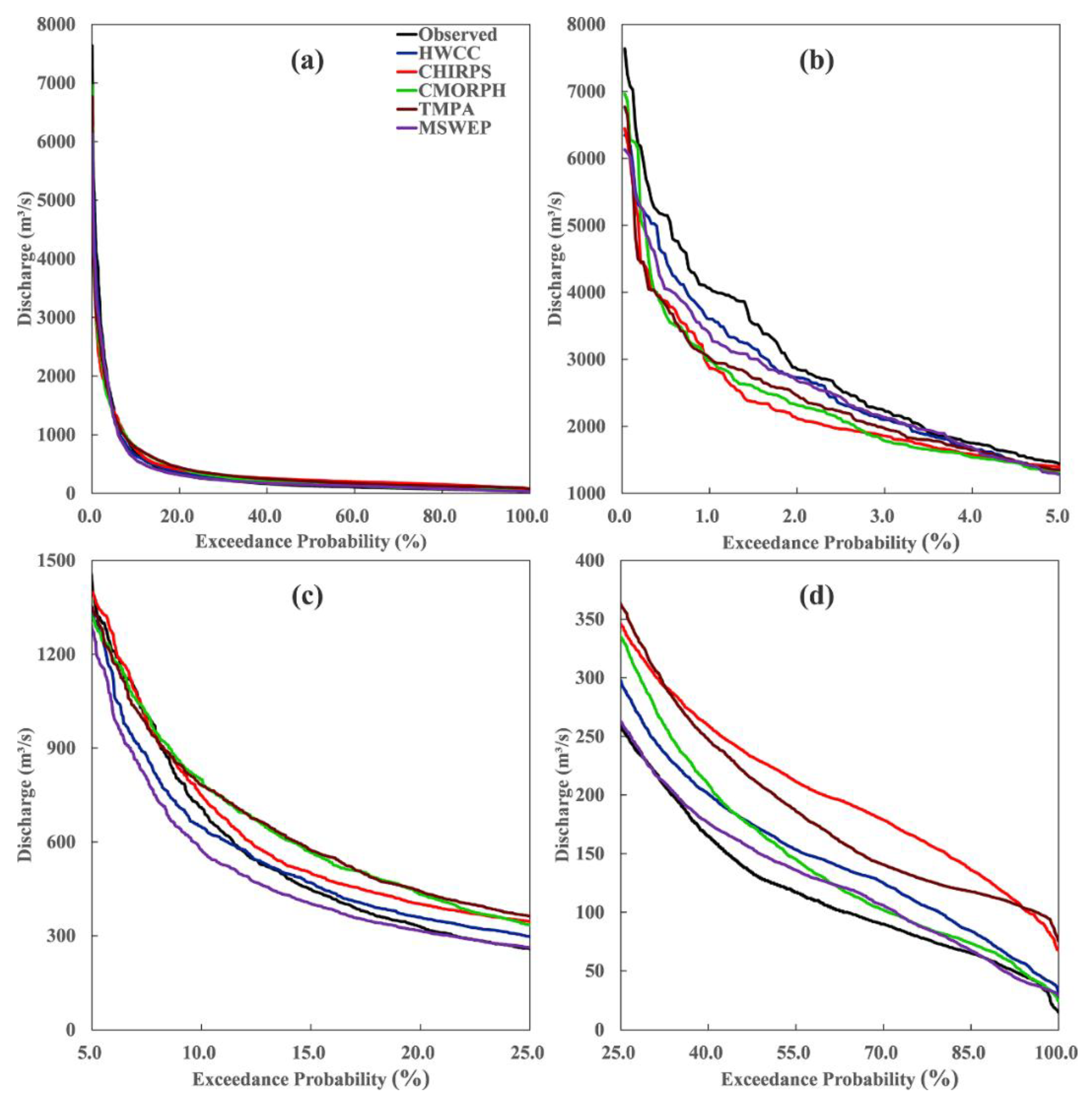
The HWCC forced simulation (Figure 7) and simulated streamflow are driven by the four QPEs under Scenario II (Figure 8) show an underestimation at the high streamflow and an overestimation at the low streamflow. The exceedance probability plots (Figure 9) are presented to further validate the performance of the four QPEs products at different exceedance probabilities. When the exceedance frequencies are less than 5.0%, all simulations underestimate the streamflow. Generally, HWCC yields the least underestimation, followed by MSWEP in this frequency interval. When the exceedance frequencies increase and exceed 5.0%, the streamflow simulated by CHIRPS, CMORPH, and TMPA gradually approaches and then exceeds the observed streamflow. The higher accuracy is concentrated in a small frequency range from 5.0 to 10.0%. HWCC forced simulation gradually exceeds the observed streamflow when the exceedance frequency is about 12.0% and presents its best performance with an exceedance frequency range from 10.0 to 17.5%. MSWEP performs best when the exceedance frequency is beyond 20%, but the streamflow simulated by MSWEP consistently underestimates the observed streamflow until the exceedance frequency is above 25%.
4.3. Evaluation of the Soil Moisture Simulations under Two Parameterization Scenarios
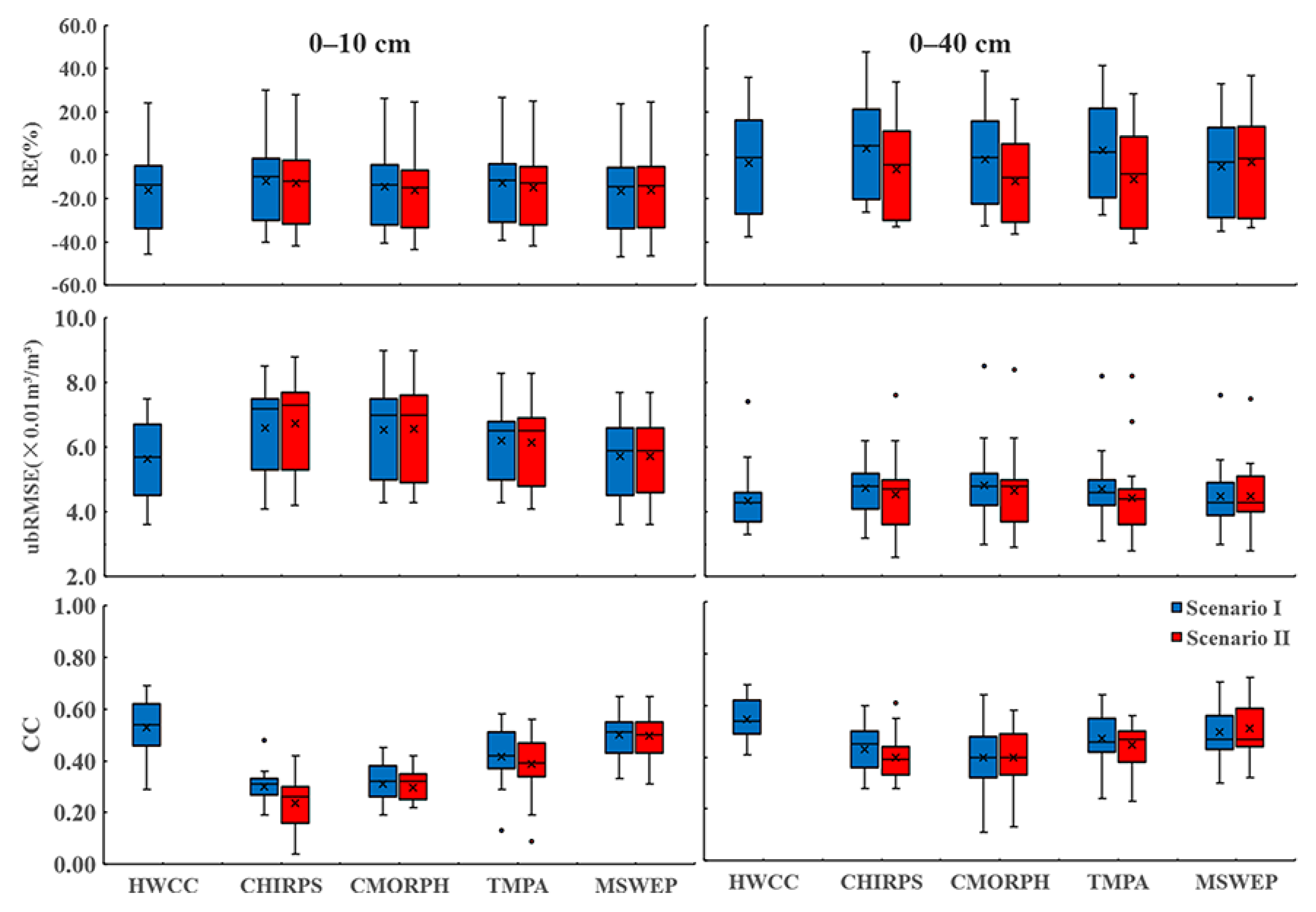
In situ soil moisture data from January 2008 to December 2010 were adopted to further evaluate the hydrological utility of different precipitation products. The box plots of the evaluation metrics for soil moisture at depths of 0–10 cm and 0–40 cm under two scenarios are presented in Figure 10. The HWCC and QPEs forced simulations significantly underestimate the soil moisture of the two soil depths under Scenario I. In addition, there is almost no difference between the REs of simulated soil moisture with different forcing precipitation, which indicates that the REs of the simulated soil moisture has little to do with forcing precipitation. Overall, the soil moisture simulated by HWCC with the least ubRMSE (the average ubRMSE is 0.056 and 0.043 m³/m³ at depths of 0–10 cm and 0–40 cm, respectively) and MSWEP is subordinate with a slightly higher ubRMSE of 0.057 and 0.045 m³/m³, respectively. CMORPH and CHIRPS are the worst performers, especially at a depth of 0–10 cm. Compared with the results for the depth of 0–10 cm, the ubRMSE of soil moisture simulated at a depth of 0–40 cm is significantly reduced. Furthermore, the difference in the ubRMSE of simulated soil moisture at a depth of 0–40 cm with different forcing precipitation products is relatively small. The CC of simulated and observed soil moisture at a depth of 0–40 cm is slightly better than that at 0–10 cm, except for MSWEP. HWCC performs best with the highest CC (the average CC is 0.53 and 0.55 at depths of 0–10 cm and 0–40 cm, respectively), followed by MSWEP (both are 0.50). Similarly, CHIRPS and CMORPH exhibit worse performances with lower CC compared with MSWEP and TMPA. With respect to the ubRMSE and CC, improving the precision of precipitation can effectively improve the precision of simulated soil moisture, especially at a depth of 0–10 cm, which indicates that the results of the simulated soil moisture at a depth of 0–10 cm are more sensitive to the accuracy of the forcing precipitation than that at a depth of 0–40 cm.
Unlike the results of simulated streamflow, the accuracy of simulated soil moisture under Scenario II seems to not notably improve compared with the simulations under Scenario I. Specifically, both the ubRMSE and CC of simulated soil moisture under Scenario II are slightly inferior to the results of Scenario I at a depth of 0–10 cm. Regarding the simulated results at a depth of 0–40 cm, both the ubRMSE and CC of simulated soil moisture under Scenario II are slightly lower than the results of Scenario I, except for the CC forced by MSWEP and CMORPH. Generally, MSWEP shows the best performance among the four QPEs in terms of simulated soil moisture under Scenario II; TMPA takes the second place, CHIRPS and CMORPH generally perform poorly, which is consistent with the results under Scenario I.
5. Discussion
The IR data measured from geostationary satellites and microwave (MV) data measured from low earth orbiting satellites are the main data sources for SPPs. Generally, SPPs are from IR data with fine temporal resolutions but with less accuracy. The MV data provide direct and accurate precipitation estimates, however, at the cost of coarse temporal resolution [41,43]. Generally, CHIRPS performs unsatisfactorily compared with TMPA and CMORPH, which is probably due to the fact that CHIRPS is mainly based on IR data, while CMORPH and TMPA combined IR and MV data. The main difference between CMORPH and TMPA is the gauge adjustment algorithm adopted in these two datasets. To develop CMORPH, the probability density function (PDF) matching against the CPC unified daily gauge analysis was used to adjust the biases. Monthly GPCC rain gauge analyses and inverse-error-variance weighting were used for the TMPA to adjust the biases. However, TMPA generally outperforms CMORPH, suggesting that the PDF matching adopted in CMOPRH is not superior to the monthly gauge adjustment algorithm used in TMPA [19], probably because PDF matching does not work well with undetected precipitation. The limitation of PDF matching mentioned above may also be the reason CMORPH performs worst (with the largest FBI and FAR and lowest ETS) in terms of the statistical scores for no rain events, which further leads to CMORPH being dominated by a significant negative RE.
MSWEP has the best performance compared with the other three QPEs, except for the significant negative RE. Tong et al. [32] pointed out that SPPs are most accurate during summer and at lower latitudes, while the atmospheric model reanalysis datasets perform better than the SPPs during winter and at higher latitudes. The optimal merging of the gauge, satellite, and reanalysis precipitation estimates complements the advantages of the three different data sources. Moreover, the finer spatial resolution of MSWEP compared with the other three QPEs provides a unique advantage over the other QPEs. The merged precipitation products MSWEP not only performs better than the other three QPEs but also, to some extent, makes up for the lack of accuracy of the single precipitation product varying depending on the seasons (in terms of CC showed in Table 3). However, MSWEP still has larger uncertainties in mountain areas, the same as SPPs.
The streamflow modeling results under Scenario I reveal that the RE of simulated streamflow mainly depends on RE of precipitation estimates. Due to the highly nonlinear rainfall–runoff response, any overestimation/underestimation of precipitation estimates can be transformed into a larger overestimation/underestimation in the simulated streamflow [7,32,44]. Specifically, the grid-averaged RE of precipitation estimates from CHIRPS and TMPA is 7.5% and 10.6%, respectively, resulting in a 14.4% and 21.0% overestimation of the streamflow simulations from 2002 to 2010. Similarly, the grid–averaged RE of precipitation estimates from CMORPH and MSWEP is −2.5% and −6.0%, respectively, resulting in an 8.2% and 17.2% underestimation of streamflow simulations from 2002 to 2010. However, the impact of the RE of precipitation estimates on the simulated streamflow is diminished under Scenario II (the RE of simulated streamflow forced by CHIRPS, CMORPH, TMPA, and MSWEP is 10.7%, 1.9%, 10.6% and −7.4%, respectively), mainly because the model parameters may change according to the precipitation input to match the streamflow. Thus, the model parameters recalibrated under Scenario II are more suitable for the corresponding precipitation products for streamflow simulation. Among the hydrological parameters of the VIC model, the shape of the variable infiltration capacity curve (B) and the depth of the three soil layers (d1, d2, and d3) are the most influential factors on streamflow and soil moisture simulation. An increase of B tends to enhance streamflow production. Soil thickness mainly controls the maximum moisture storage capacity. The thicker soil depths have higher moisture storage capacities, thus, more evaporation loss and less streamflow production. Three base flow parameters (Dsmax, Ds, and Ws) determine how quickly the water storage in the third layer evacuates and are generally less sensitive than the parameters B and the thicker soil depths [45]. The MSWEP precipitation estimate decreases d2 after recalibration compared with the model parameters under Scenario I (Table 6) to retain less soil moisture and enhance streamflow production. The model parameters recalibrated by MSWEP are mostly close to the results of HWCC, which further indicates that MSWEP has satisfactory accuracy. The recalibrated results of CHIRPS have a smaller B and thicker soil thickness with the potential purpose to offset the positive RE of precipitation estimates. The CMORPH and TMPA precipitation estimate increases B and soil thickness tends to yield more streamflow and retain more soil moisture. However, the soil thickness recalibrated by TMPA increases significantly, which means that more precipitation is stored in the soil, further reducing the RE of the simulated streamflow. Although the increase of B recalibrated by CMORPH can compensate for the negative RE of precipitation estimates, the decrease of the seasonal peak discharge caused by the increase of the soil thickness may be one of the main reasons for the worst performance of CMORPH during the validation period under Scenario II.
The model structure, forcing data, and parameters are the main factors affecting the accuracy of soil moisture simulation [46,47], which has been proved by the results of this study. There are little differences between the RE of the simulated soil moisture with different forcing precipitation products, which indicates that the existing systematic errors of the VIC model are probably the main causes of the RE of simulated soil moisture. However, the dynamic change tendency of the simulated soil moisture driven by precipitation with higher precision is more consistent with the observed results (with lower ubRMSE and higher CC). This demonstrates that rainfall forcing data are one of the important factors influencing the accuracy of simulated soil moisture. In this study, the model parameters are calibrated in terms of the highest NSCE between the simulated and observed streamflow at the watershed outlet, without considering the simulation results for other hydrological variables (such as soil moisture). Therefore, the parameters determined by this method may not reasonably reflect the actual conditions of the study area. Comparatively speaking, the parameters calibrated using a relatively dense network of rain gauge stations (Scenario I) can be considered as the best possible approximation of watershed hydrological features [44]. In Scenario II, these parameters were recalibrated with individual QPEs, which takes into account the potential impacts of input uncertainty on the streamflow simulations [19]. Thus, with the recalibrated model parameters, the streamflow simulations are likely to produce more accurate results than the case under Scenario I. However, the recalibrated model parameters may not reflect watershed hydrological features well, which results in the improvements of the simulated soil moisture under Scenario II being insignificant or even worse than the results under Scenario I, indicating that the model parameters may be the major factors influencing the accuracy of the simulated soil moisture.
The evaluation of the hydrological simulation capability in this study partly indicates that the merged precipitation product, MSWEP, has great potential to be a reliable dataset for conducting long-term hydrological studies compared with the three SPPs. However, the simulated results using HWCC are closer to observations than that using MSWEP, which may be due to two reasons: (1) the layout of rain gauge stations used in this study takes into consideration the factors of rainstorm and flood formation, so, it can reflect the precipitation characteristics of the study area well and it is suitable for hydrological simulation; and (2) the satellite-based precipitation estimates are inevitably subject to errors resulting from indirect measurements although rain gauge information is incorporated to reduce biases, but due to the insufficient gauge observations in the bias–corrected or merging process, the uncertainty in the satellite-based precipitation estimate has not been fully solved.
6. Conclusions
This study provides a comprehensive assessment of the newly merged precipitation product MSWEP and three typical SPPs based on rain gauge observations and the VIC hydrologic model in the upper Huaihe River basin. The primary conclusions can be summarized as follows:
- (1)
- All four QPEs are subject to significant errors, although the spatial patterns of average annual precipitation are generally consistent with the rain gauge observations. Specifically, CHIRPS and TMPA generally overestimate precipitation; however, CMORPH and MSWEP generally underestimate precipitation. Overall, MSWEP performs best, TMPA takes the second place, and CHIRPS exhibits a relatively poor performance. The contribution of the random error generally larger than the systematic error of the four QPEs and the spatial distributions of the two error components are closely related to the topography. Simultaneously, all QPEs are prone to underestimate the precipitation in regions daily precipitation with larger temporal variability (higher standard deviation) and the precipitation detection capabilities of QPEs decrease with increasing precipitation magnitude.
- (2)
- Under Scenario I (model parameters calibrated by rain gauge observations), similar to the results of the statistical evaluation, CHIRPS and TMPA forced simulations tend to overestimate streamflow, while serious underestimations are observed in the streamflow simulations of both CMORPH and MSWEP, which indicates that the RE of simulated streamflow is greatly affected by the RE of the forcing precipitation products. MSWEP outperforms the other three QPEs (NSCE lower than 0.70) with the highest NSCE (NSCE = 0.87 and 0.74 for the calibration and validation period, respectively), implying that the MSWEP products could better reveal the precipitation spatial pattern.
- (3)
- Under scenario II (model parameters separately recalibrated using the QPEs), all simulations are improved compared with Scenario I. Similarly, MSWEP exhibits the best performance, followed by TMPA. CHIRPS and CMORPH forced simulation performed poorly. The influence of the RE of the QPEs on simulated streamflow may be mitigated by recalibrating the parameters with the corresponding QPEs. Furthermore, all QPE forced simulations underestimate the observed streamflow with exceedance probabilities less than 5.0% whilst they overestimate the observed streamflow with exceedance probabilities of more than 30.0%. HWCC performs best with exceedance probabilities that are less than 5.0%, followed by MSWEP, while MSWEP performs best with exceedance probabilities of more than 20.0%.
- (4)
- Under the two scenarios, the difference of RE of soil moisture simulated by different precipitation products is insignificant, implying that the existing systematic error of the VIC model is probably the main cause of the RE of simulated soil moisture. However, with increasing accuracy of the forcing precipitation products, the dynamic changes of the simulated soil moisture become more consistent with the measured results (lower ubRMSE and higher CC), especially for the results at a depth of 0–10 cm. Generally, the soil moisture simulated by different precipitation products at a depth of 0–40 cm is slightly better than the results for the depth of 0–10 cm. Unlike the simulated discharge, the accuracy of the simulated soil moisture under Scenario II is even worse than the results under Scenario I, which indicates that the model parameters are the main factors influencing the accuracy of the simulated soil moisture, in addition to the forcing data.
In summary, the merged precipitation product MSWEP presents a satisfactory performance both in the statistical evaluation and hydrological simulation in the study area, indicating the large potential to substitute rain gauge observations. However, there are still some limitations in the MSWEP product, for example, the MSWEP product has great uncertainty in mountainous regions the same as SPPs. Future studies are needed to further contrastive evaluation of the applicability of MSWEP and relevant SPPs over different climate zones, and then improve the data fusion scheme according to the error characteristics of MSWEP, to obtain more accurate precipitation estimates.
Author Contributions
All authors contributed extensively to the work presented in this paper. Z.W. designed the framework of this study and wrote the paper. Z.X. conducted the analysis and wrote the paper. F.W. contributed to the writing of the paper. H.H. provided constructive comments and revised the paper. J.Z. collected observation data and revised the paper. X.W. and Z.L. revised the paper.
Funding
This research was funded by the National Key Research and Development Project (No. 2017YFC1502403), the National Science Foundation of China (Grant Nos. 51779071, 51579065), the Fundamental Research Funds for the Central Universities (Grant No. 2017B10514), Central Public Welfare Operations for Basic Scientific Research of Research Institute (Grant No. HKY-JBYW-2017-12) and Water Science and Technology Project of Jiangsu Province (2017007).
Conflicts of Interest
The authors declare no conflict of interest.
References
- Beck, H.E.; Vergopolan, N.; Pan, M.; Levizzani, V.; van Dijk, A.I.J.M.; Weedon, G.P.; Brocca, L.; Pappenberger, F.; Huffman, G.J.; Wood, E.F. Global-scale evaluation of 22 precipitation datasets using gauge observations and hydrological modeling. Hydrol. Earth Syst. Sci. 2017, 21, 6201–6217. [Google Scholar] [CrossRef]
- Liu, X.; Yang, T.; Hsu, K.; Liu, C.; Sorooshian, S. Evaluating the streamflow simulation capability of persiann-cdr daily rainfall products in two river basins on the tibetan plateau. Hydrol. Earth Syst. Sci. 2017, 21, 169–181. [Google Scholar] [CrossRef]
- Sorooshian, S.; AghaKouchak, A.; Arkin, P.; Eylander, J.; Foufoula-Georgiou, E.; Harmon, R.; Hendrickx, J.M.H.; Imam, B.; Kuligowski, R.; Skahill, B.; et al. Advanced concepts on remote sensing of precipitation at multiple scales. Bull. Am. Meteorol. Soc. 2011, 92, 1353–1357. [Google Scholar] [CrossRef]
- Prakash, S.; Mitra, A.K.; AghaKouchak, A.; Pai, D.S. Error characterization of trmm multisatellite precipitation analysis (tmpa-3b42) products over india for different seasons. J. Hydrol. 2015, 529, 1302–1312. [Google Scholar] [CrossRef]
- Xue, X.; Hong, Y.; Limaye, A.S.; Gourley, J.J.; Huffman, G.J.; Khan, S.I.; Dorji, C.; Chen, S. Statistical and hydrological evaluation of trmm-based multi-satellite precipitation analysis over the wangchu basin of bhutan: Are the latest satellite precipitation products 3b42v7 ready for use in ungauged basins? J. Hydrol. 2013, 499, 91–99. [Google Scholar] [CrossRef]
- Duethmann, D.; Zimmer, J.; Gafurov, A.; Guentner, A.; Kriegel, D.; Merz, B.; Vorogushyn, S. Evaluation of areal precipitation estimates based on downscaled reanalysis and station data by hydrological modelling. Hydrol. Earth Syst. Sci. 2013, 17, 2415–2434. [Google Scholar] [CrossRef]
- Zhu, Q.; Xuan, W.; Liu, L.; Xu, Y.-P. Evaluation and hydrological application of precipitation estimates derived from persiann-cdr, trmm 3b42v7, and ncep-cfsr over humid regions in china. Hydrol. Process. 2016, 30, 3061–3083. [Google Scholar] [CrossRef]
- Funk, C.; Peterson, P.; Landsfeld, M.; Pedreros, D.; Verdin, J.; Shukla, S.; Husak, G.; Rowland, J.; Harrison, L.; Hoell, A.; et al. The climate hazards infrared precipitation with stations—A new environmental record for monitoring extremes. Sci. Data 2015, 2, 150066. [Google Scholar] [CrossRef] [PubMed]
- Joyce, R.J.; Janowiak, J.E.; Arkin, P.A.; Xie, P.P. Cmorph: A method that produces global precipitation estimates from passive microwave and infrared data at high spatial and temporal resolution. J. Hydrometeorol. 2004, 5, 487–503. [Google Scholar] [CrossRef]
- Huffman, G.J.; Adler, R.F.; Bolvin, D.T.; Gu, G.; Nelkin, E.J.; Bowman, K.P.; Hong, Y.; Stocker, E.F.; Wolff, D.B. The trmm multisatellite precipitation analysis (tmpa): Quasi-global, multiyear, combined-sensor precipitation estimates at fine scales. J. Hydrometeorol. 2007, 8, 38–55. [Google Scholar] [CrossRef]
- Ushio, T.; Sasashige, K.; Kubota, T.; Shige, S.; Okamoto, K.; Aonashi, K.; Inoue, T.; Takahashi, N.; Iguchi, T.; Kachi, M.; et al. A kalman filter approach to the global satellite mapping of precipitation (gsmap) from combined passive microwave and infrared radiometric data. J. Meteorol. Soc. Jpn. 2009, 87A, 137–151. [Google Scholar] [CrossRef]
- Huffman, G.J.; Bolvin, D.T.; Braithwaite, D.; Hsu, K.; Joyce, R.; Kidd, C.; Sorooshian, S.; Xie, P.; Yoo, S.H. Developing the integrated multi-satellite retrievals for gpm (imerg). In Proceedings of the EGU General Assembly Conference, Vienna, Austria, 22–27 April 2012. [Google Scholar]
- Beria, H.; Nanda, T.; Bisht, D.S.; Chatterjee, C. Does the gpm mission improve the systematic error component in satellite rainfall estimates over trmm? An evaluation at a pan-india scale. Hydrol. Earth Syst. Sci. 2017, 21, 6117–6134. [Google Scholar] [CrossRef]
- Wang, Z.; Zhong, R.; Lai, C.; Chen, J. Evaluation of the gpm imerg satellite-based precipitation products and the hydrological utility. Atmosp. Res. 2017, 196, 151–163. [Google Scholar] [CrossRef]
- Prakash, S.; Mitra, A.K.; Aghakouchak, A.; Liu, Z.; Norouzi, H.; Pai, D.S. A preliminary assessment of gpm-based multi-satellite precipitation estimates over a monsoon dominated region. J. Hydrol. 2016, 556, 865–876. [Google Scholar] [CrossRef]
- Zhao, H.; Yang, B.; Yang, S.; Huang, Y.; Dong, G.; Bai, J.; Wang, Z. Systematical estimation of gpm-based global satellite mapping of precipitation products over china. Atmosp. Res. 2018, 201, 206–217. [Google Scholar] [CrossRef]
- Zubieta, R.; Getirana, A.; Espinoza, J.C.; Lavado, W. Impacts of satellite-based precipitation datasets on rainfall-runoff modeling of the western amazon basin of peru and ecuador. J. Hydrol. 2015, 528, 599–612. [Google Scholar] [CrossRef]
- Zulkafli, Z.; Buytaert, W.; Onof, C.; Manz, B.; Tarnavsky, E.; Lavado, W.; Guyot, J.-L. A comparative performance analysis of trmm 3b42 (tmpa) versions 6 and 7 for hydrological applications over andean-amazon river basins. J. Hydrometeorol. 2014, 15, 581–592. [Google Scholar] [CrossRef]
- Sun, R.; Yuan, H.; Liu, X.; Jiang, X. Evaluation of the latest satellite-gauge precipitation products and their hydrologic applications over the huaihe river basin. J. Hydrol. 2016, 536, 302–319. [Google Scholar] [CrossRef]
- Gao, Z.; Long, D.; Tang, G.; Zeng, C.; Huang, J.; Hong, Y. Assessing the potential of satellite-based precipitation estimates for flood frequency analysis in ungauged or poorly gauged tributaries of China’s yangtze river basin. J. Hydrol. 2017, 550, 478–496. [Google Scholar] [CrossRef]
- Sahoo, A.K.; Sheffield, J.; Pan, M.; Wood, E.F. Evaluation of the tropical rainfall measuring mission multi-satellite precipitation analysis (tmpa) for assessment of large-scale meteorological drought. Remote Sens. Environ. 2015, 159, 181–193. [Google Scholar] [CrossRef]
- Bayissa, Y.; Tadesse, T.; Demisse, G.; Shiferaw, A. Evaluation of satellite-based rainfall estimates and application to monitor meteorological drought for the upper blue nile basin, ethiopia. Remote Sens. 2017, 9, 669. [Google Scholar] [CrossRef]
- Tote, C.; Patricio, D.; Boogaard, H.; van der Wijngaart, R.; Tarnavsky, E.; Funk, C. Evaluation of satellite rainfall estimates for drought and flood monitoring in mozambique. Remote Sens. 2015, 7, 1758–1776. [Google Scholar] [CrossRef]
- Yang, N.; Zhang, K.; Hong, Y.; Zhao, Q.; Huang, Q.; Xu, Y.; Xue, X.; Chen, S. Evaluation of the trmm multisatellite precipitation analysis and its applicability in supporting reservoir operation and water resources management in hanjiang basin, China. J. Hydrol. 2017, 549, 313–325. [Google Scholar] [CrossRef]
- Maggioni, V.; Meyers, P.C.; Robinson, M.D. A review of merged high-resolution satellite precipitation product accuracy during the tropical rainfall measuring mission (trmm) era. J. Hydrometeorol. 2016, 17, 1101–1117. [Google Scholar] [CrossRef]
- Zhao, H.; Yang, S.; You, S.; Huang, Y.; Wang, Q.; Zhou, Q. Comprehensive evaluation of two successive v3 and v4 imerg final run precipitation products over mainland China. Remote Sens. 2018, 10, 34. [Google Scholar] [CrossRef]
- He, Y.; Zhang, Y.; Kuligowski, R.; Cifelli, R.; Kitzmiller, D. Incorporating satellite precipitation estimates into a radar-gauge multi-sensor precipitation estimation algorithm. Remote Sens. 2018, 10, 106. [Google Scholar] [CrossRef]
- Beck, H.E.; van Dijk, A.I.J.M.; Levizzani, V.; Schellekens, J.; Miralles, D.G.; Martens, B.; de Roo, A. Mswep: 3-hourly 0.25 degrees global gridded precipitation (1979–2015) by merging gauge, satellite, and reanalysis data. Hydrol. Earth Syst. Sci. 2017, 21, 589–615. [Google Scholar] [CrossRef]
- Boudevillain, B.; Delrieu, G.; Wijbrans, A.; Confoland, A. A high-resolution rainfall re-analysis based on radar-raingauge merging in the cevennes-vivarais region, France. J. Hydrol. 2016, 541, 14–23. [Google Scholar] [CrossRef]
- Ciabatta, L.; Brocca, L.; Massari, C.; Moramarco, T.; Gabellani, S.; Puca, S.; Wagner, W. Rainfall-runoff modelling by using sm2rain-derived and state-of-the-art satellite rainfall products over italy. Int. J. Appl. Earth Obs. Geoinform. 2016, 48, 163–173. [Google Scholar] [CrossRef]
- Massari, C.; Camici, S.; Ciabatta, L.; Brocca, L. Exploiting satellite-based surface soil moisture for flood forecasting in the mediterranean area: State update versus rainfall correction. Remote Sens. 2018, 10, 292. [Google Scholar] [CrossRef]
- Tong, K.; Su, F.; Yang, D.; Hao, Z. Evaluation of satellite precipitation retrievals and their potential utilities in hydrologic modeling over the tibetan plateau. J. Hydrol. 2014, 519, 423–437. [Google Scholar] [CrossRef]
- Wu, Z.Y.; Lu, G.H.; Wen, L.; Lin, C.A. Reconstructing and analyzing china’s fifty-nine year (1951–2009) drought history using hydrological model simulation. Hydrol. Earth Syst. Sci. 2011, 15, 2881–2894. [Google Scholar] [CrossRef] [Green Version]
- Wu, J.; Lu, G.; Wu, Z. Flood forecasts based on multi-model ensemble precipitation forecasting using a coupled atmospheric-hydrological modeling system. Nat. Hazards 2014, 74, 325–340. [Google Scholar] [CrossRef]
- Liang, X.; Wood, E.F.; Lettenmaier, D.P. Surface soil moisture parameterization of the vic-2l model: Evaluation and modification. Glob. Planet. Chang. 1996, 13, 195–206. [Google Scholar] [CrossRef]
- Hansen, M.C.; Defries, R.S.; Townshend, J.R.G.; Sohlberg, R. Global land cover classification at 1km spatial resolution using a classification tree approach. Int. J. Remote Sens. 2000, 21, 1331–1364. [Google Scholar] [CrossRef]
- Reynolds, C.A.; Jackson, T.J.; Rawls, W.J. Estimating soil water-holding capacities by linking the food and agriculture organization soil map of the world with global pedon databases and continuous pedotransfer functions. Water Resour. Res. 2000, 36, 3653–3662. [Google Scholar] [CrossRef]
- Rosenbrock, H.H. An automatic method for finding the greatest or least value of a function. Comput. J. 1960, 3, 175–184. [Google Scholar] [CrossRef]
- Sun, Y.; Huang, S.; Ma, J.; Li, J.; Li, X.; Wang, H.; Chen, S.; Zang, W. Preliminary evaluation of the smap radiometer soil moisture product over china using in situ data. Remote Sens. 2017, 9, 292. [Google Scholar] [CrossRef]
- Bai, L.; Shi, C.; Li, L.; Yang, Y.; Wu, J. Accuracy of chirps satellite-rainfall products over mainland China. Remote Sens. 2018, 10, 362. [Google Scholar] [CrossRef]
- Duan, Z.; Liu, J.; Tuo, Y.; Chiogna, G.; Disse, M. Evaluation of eight high spatial resolution gridded precipitation products in adige basin (Italy) at multiple temporal and spatial scales. Sci. Total Environ. 2016, 573, 1536–1553. [Google Scholar] [CrossRef] [PubMed]
- Alijanian, M.; Rakhshandehroo, G.R.; Mishra, A.K.; Dehghani, M. Evaluation of satellite rainfall climatology using cmorph, persiann-cdr, persiann, trmm, mswep over Iran. Int. J. Climatol. 2017, 37, 4896–4914. [Google Scholar] [CrossRef]
- Serrat-Capdevila, A.; Merino, M.; Valdes, J.B.; Durcik, M. Evaluation of the performance of three satellite precipitation products over Africa. Remote Sens. 2016, 8, 836. [Google Scholar] [CrossRef]
- Yuan, F.; Zhang, L.; Win, K.W.W.; Ren, L.; Zhao, C.; Zhu, Y.; Jiang, S.; Liu, Y. Assessment of gpm and trmm multi-satellite precipitation products in streamflow simulations in a data-sparse mountainous watershed in Myanmar. Remote Sens. 2017, 9, 302. [Google Scholar] [CrossRef]
- Zhang, L.; Su, F.; Yang, D.; Hao, Z.; Tong, K. Discharge regime and simulation for the upstream of major rivers over tibetan plateau. J. Geophys. Res. Atmosp 2013, 118, 8500–8518. [Google Scholar] [CrossRef]
- Mo, K.C.; Lettenmaier, D.P. Objective drought classification using multiple land surface models. J. Hydrometeorol. 2014, 15, 990–1010. [Google Scholar] [CrossRef]
- Tramblay, Y.; Bouvier, C.; Ayral, P.A.; Marchandise, A. Impact of rainfall spatial distribution on rainfall-runoff modelling efficiency and initial soil moisture conditions estimation. Nat. Hazards Earth Syst. Sci. 2011, 11, 157–170. [Google Scholar] [CrossRef]
Figure 1.
The location of the upper region of the Wangjiaba Station in the Huaihe River Basin and the distribution of stations used in this study.
Figure 1.
The location of the upper region of the Wangjiaba Station in the Huaihe River Basin and the distribution of stations used in this study.

Figure 2.
The spatial distribution of the average annual precipitation (mm/year) of daily precipitation interpolated from 57 rain gauges (HWCC), Climate Hazards Group Infrared Precipitation with Station data Version2.0 (CHIRPS), NOAA’s Climate Prediction Center (CPC) MORPHing technique bias-corrected product (CMORPH), NASA’s Tropical Rainfall Measuring Mission (TRMM) Multi-satellite Precipitation Analysis 3B42 Version 7 (TMPA), and Multi-Source Weighted-Ensemble Precipitation Version 2.1 (MSWEP) from 2000 to 2010.

Figure 3.
The spatial patterns of the relative error (RE) (%), root mean squared error (RMSE) (mm/day), and correlation coefficient (CC) of the four quantitative precipitation estimates (QPEs) and HWCC (from top to bottom) from 2000 to 2010.
Figure 3.
The spatial patterns of the relative error (RE) (%), root mean squared error (RMSE) (mm/day), and correlation coefficient (CC) of the four quantitative precipitation estimates (QPEs) and HWCC (from top to bottom) from 2000 to 2010.
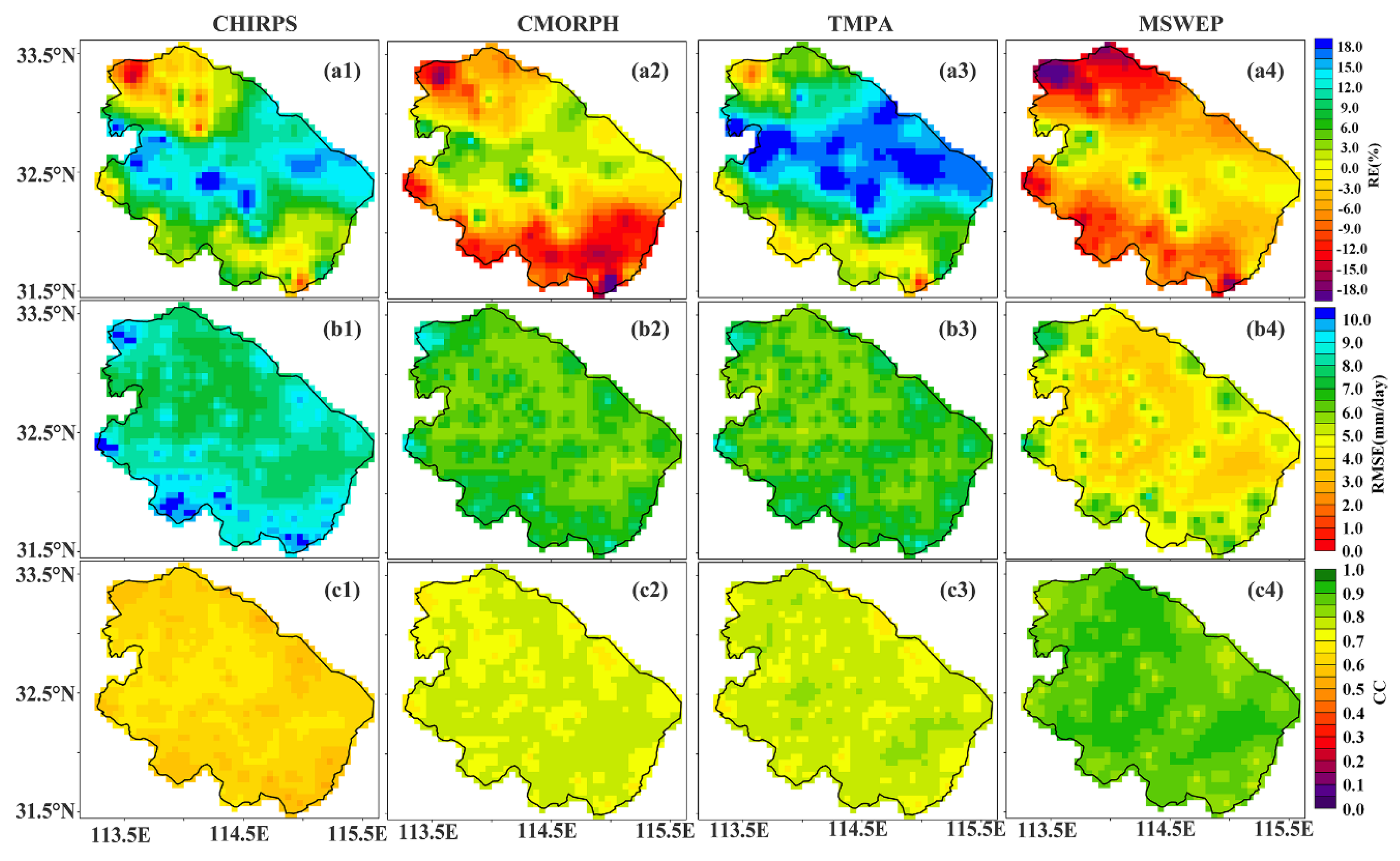
Figure 4.
The contribution of systematic error (a1–a4) and random error (b1–b4) components to the mean square error of the four QPEs from 2000 to 2010.
Figure 4.
The contribution of systematic error (a1–a4) and random error (b1–b4) components to the mean square error of the four QPEs from 2000 to 2010.

Figure 5.
The scatter plots of the standard deviation (SD) versus RE for the four QPEs.
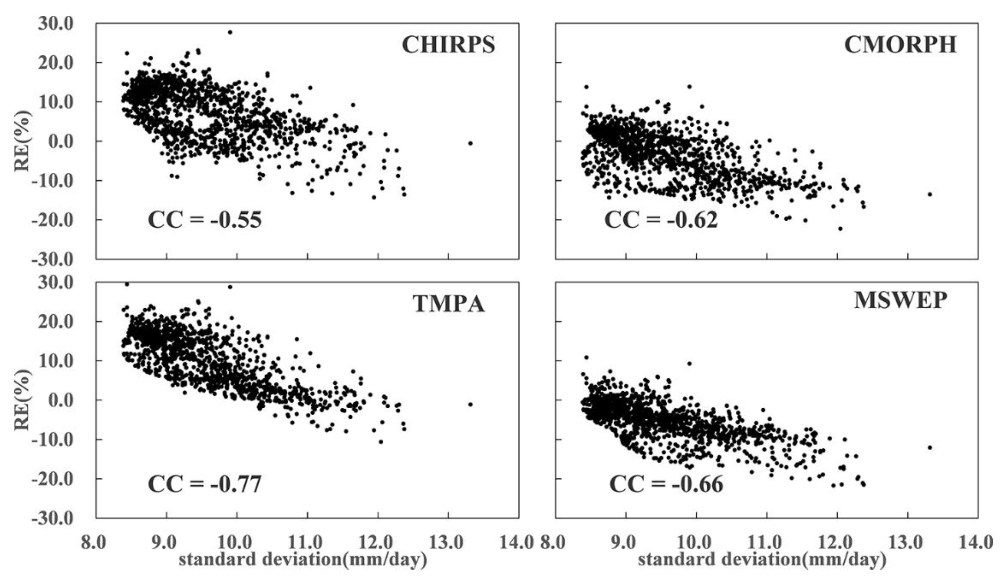
Figure 6.
The four statistical scores of different QPEs versus HWCC at different precipitation thresholds from 2000 to 2010.
Figure 6.
The four statistical scores of different QPEs versus HWCC at different precipitation thresholds from 2000 to 2010.
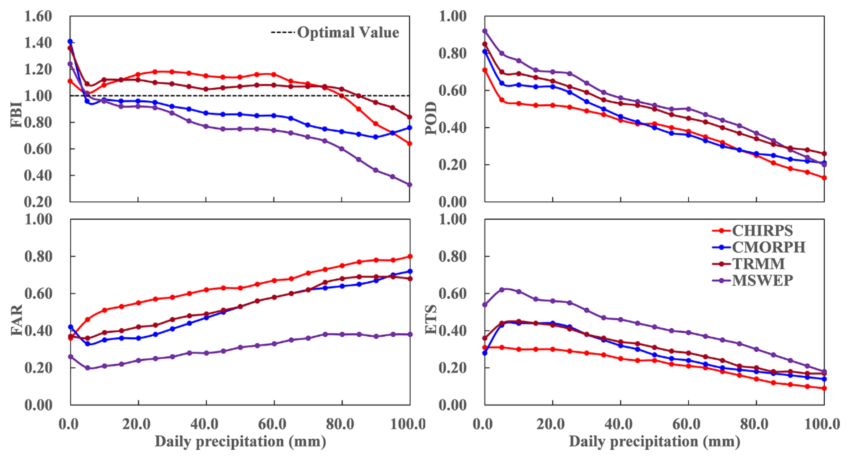
Figure 7.
The comparison between the daily discharge simulated using HWCC precipitation and the observed data at the Wangjiaba Station.
Figure 7.
The comparison between the daily discharge simulated using HWCC precipitation and the observed data at the Wangjiaba Station.

Figure 8.
The comparison between the observed and simulated discharge of CHIRPS, CMORPH, TMAP, and MSWEP at the Wangjiaba Station under Scenario II.
Figure 8.
The comparison between the observed and simulated discharge of CHIRPS, CMORPH, TMAP, and MSWEP at the Wangjiaba Station under Scenario II.

Figure 9.
The exceedance probabilities of the daily streamflow during the whole period under Scenario II: (a) all frequencies; (b) frequencies below 5.0%; (c) frequencies ranging from 5.0 to 25.0%; (d) frequencies exceeding 25.0%.
Figure 9.
The exceedance probabilities of the daily streamflow during the whole period under Scenario II: (a) all frequencies; (b) frequencies below 5.0%; (c) frequencies ranging from 5.0 to 25.0%; (d) frequencies exceeding 25.0%.

Figure 10.
The box plots of the evaluation metrics for the soil moisture at depths of 0–10 cm and 0–40 cm under two scenarios.
Figure 10.
The box plots of the evaluation metrics for the soil moisture at depths of 0–10 cm and 0–40 cm under two scenarios.


Table 1.
The summary of the precipitation datasets used in this study.
| Full Name and Details | Short Name | Data Sources | Spatiotemporal Resolution Used in This Study |
|---|---|---|---|
| Climate Hazards Group Infrared Precipitation with Station data Version2.0 (CHIRPS V2.0) | CHIRPS | CHPclim, thermal infrared data, the TMPA 3B42 V7, rain gauge stations data | Daily, 0.25° |
| NOAA’s Climate Prediction Center (CPC) MORPHing technique (CMORPH) bias-corrected product (CMORPH CRT V1.0) | CMORPH | TMI, SSM/I, AMSR-E, AMSU-B, Meteosat, GOES, MTSAT and CPC | 3 hourly, 0.25° |
| NASA’s Tropical Rainfall Measuring Mission (TRMM) Multi-satellite Precipitation Analysis (TMPA) 3B42 Version 7 | TMPA | TMI, TRMM Combined Instrument, SSM/I, SSMIS, AMSR-E, MHS, AMSU-B, GEO IR and GPCC | 3 hourly, 0.25° |
| Multi-Source Weighted-Ensemble Precipitation Version 2.1(MSWEP) | MSWEP | CPC, GPCC, CMORPH, GSMaP-MVK, TMPA, ERA-Interim, JRA-55 | Daily, 0.25° |
| daily precipitation interpolated from 57 rain gauges provided by Hydrology Bureau of the Huaihe Water Conservancy Commission | HWCC | Rain gauges | Daily |
Table 2.
The list of statistical evaluation indices to evaluate the quantitative precipitation estimates (QPEs) and their hydrological applicability.
Table 2.
The list of statistical evaluation indices to evaluate the quantitative precipitation estimates (QPEs) and their hydrological applicability.
| Evaluation Indexes | Formulas | Comments | Perfect Value |
|---|---|---|---|
| RE | Si and Oi are the evaluated and observed values; and are the mean values of Si and Oi; n is the number of samples. | 0 | |
| RMSE | 0 | ||
| CC | 1 | ||
| NSCE | 1 | ||
| ubRMSE | 0 | ||
| MSEsys | Si* is defined using a linear regression error model (Si* = a × Oi + b) with a as the slope and b as the intercept. | 0 | |
| MSEran | 0 | ||
| Pm | Pm is the frequency of discharge of no less than Om; m is the number of discharge not less than Om. | ||
| FBI | NA, number of observed and detected rainfall events; NB, number of detected but not observed rainfall events; NC, number of observed but not detected rainfall events; ND, number of rainfall events that were not observed and not detected. | 1 | |
| POD | 1 | ||
| FAR | 0 | ||
| ETS | 1 |
Table 3.
The grid-averaged relative error (RE) (%),root mean squared error (RMSE) (mm/day), and correlation coefficient (CC) of the four QPEs and daily precipitation interpolated from 57 rain gauges (HWCC) for the whole period, spring, summer, autumn, and winter.
Table 3.
The grid-averaged relative error (RE) (%),root mean squared error (RMSE) (mm/day), and correlation coefficient (CC) of the four QPEs and daily precipitation interpolated from 57 rain gauges (HWCC) for the whole period, spring, summer, autumn, and winter.
| Criteria | CHIRPS | CMORPH | TMPA | MSWEP | |
|---|---|---|---|---|---|
| Whole period | RE (%) | 7.1 | −3.3 | 10.4 | −5.4 |
| RMSE (mm/day) | 8.3 | 6.5 | 6.6 | 4.5 | |
| CC | 0.63 | 0.76 | 0.77 | 0.88 | |
| Spring (MAM) | RE (%) | 1.6 | −35.7 | −0.2 | −24.6 |
| RMSE (mm/day) | 3.5 | 3.0 | 3.4 | 1.3 | |
| CC | 0.45 | 0.50 | 0.51 | 0.93 | |
| Summer (JJA) | RE (%) | 15.2 | 2.8 | 12.1 | −4.8 |
| RMSE (mm/day) | 7.4 | 4.7 | 4.7 | 3.0 | |
| CC | 0.54 | 0.80 | 0.80 | 0.91 | |
| Autumn (SON) | RE (%) | 6.0 | 1.7 | 10.7 | 1.2 |
| RMSE (mm/day) | 12.9 | 10.8 | 10.7 | 7.9 | |
| CC | 0.66 | 0.75 | 0.77 | 0.87 | |
| Winter (DJF) | RE (%) | 5.4 | −7.5 | 15.6 | −16.5 |
| RMSE (mm/day) | 6.4 | 4.5 | 4.9 | 2.7 | |
| CC | 0.58 | 0.68 | 0.73 | 0.89 |
Table 4.
The RE and Nash-Sutcliffe coefficient of Efficiency (NSCE) of the hydrological simulation results of the four QPEs under two scenarios.
Table 4.
The RE and Nash-Sutcliffe coefficient of Efficiency (NSCE) of the hydrological simulation results of the four QPEs under two scenarios.
| Precipitation Products | Scenario I | Scenario II | ||||||
|---|---|---|---|---|---|---|---|---|
| Calibration Period | Validation Period | Calibration Period | Validation Period | |||||
| RE (%) | NSCE | RE (%) | NSCE | RE (%) | NSCE | RE (%) | NSCE | |
| HWCC | 0.1 | 0.93 | 4.7 | 0.90 | ||||
| CHIRPS | 23.2 | 0.60 | 5.8 | 0.56 | 19.0 | 0.72 | −0.1 | 0.55 |
| CMORPH | 0.4 | 0.69 | −21.3 | 0.53 | 9.2 | 0.77 | −10.5 | 0.52 |
| TMPA | 30.8 | 0.66 | 19.1 | 0.69 | 18.1 | 0.79 | 1.1 | 0.73 |
| MSWEP | −12.0 | 0.87 | −19.4 | 0.74 | −4.1 | 0.89 | −11.6 | 0.78 |
Table 5.
Similar to Table 4, but for the flood season during 2002–2010.
Table 5.
Similar to Table 4, but for the flood season during 2002–2010.
| Precipitation Products | Scenario I | Scenario II | ||
|---|---|---|---|---|
| RE (%) | NSCE | RE (%) | NSCE | |
| HWCC | −14.2 | 0.94 | ||
| CHIRPS | −3.3 | 0.60 | −10.1 | 0.65 |
| CMORPH | −17.3 | 0.58 | −8.1 | 0.65 |
| TMPA | 10.0 | 0.68 | −8.4 | 0.76 |
| MSWEP | −21.2 | 0.81 | −13.4 | 0.84 |
Table 6.
The optimal model parameters of the Variable Infiltration Capacity (VIC) model under two scenarios.
Table 6.
The optimal model parameters of the Variable Infiltration Capacity (VIC) model under two scenarios.
| Parameters | Unit | Scenario I | Scenario II | |||
|---|---|---|---|---|---|---|
| CHIRPS | CMORPH | TMPA | MSWEP | |||
| B | 0.1 | 0.06 | 0.18 | 0.14 | 0.1 | |
| Ds | 0.998 | 0.092 | 0.068 | 0.035 | 0.530 | |
| Dsmax | mm | 0.5 | 10.0 | 9.0 | 13.0 | 0.5 |
| Ws | 0.99 | 0.99 | 0.70 | 0.99 | 0.72 | |
| d1 | m | 0.1 | 0.1 | 0.1 | 0.1 | 0.1 |
| d2 | m | 0.50 | 0.60 | 0.58 | 1.2 | 0.42 |
| d3 | m | 0.11 | 0.37 | 0.15 | 0.81 | 0.11 |
© 2018 by the authors. Licensee MDPI, Basel, Switzerland. This article is an open access article distributed under the terms and conditions of the Creative Commons Attribution (CC BY) license (http://creativecommons.org/licenses/by/4.0/).
Share and Cite
MDPI and ACS Style
Wu, Z.; Xu, Z.; Wang, F.; He, H.; Zhou, J.; Wu, X.; Liu, Z. Hydrologic Evaluation of Multi-Source Satellite Precipitation Products for the Upper Huaihe River Basin, China. Remote Sens. 2018, 10, 840. https://doi.org/10.3390/rs10060840
AMA Style
Wu Z, Xu Z, Wang F, He H, Zhou J, Wu X, Liu Z. Hydrologic Evaluation of Multi-Source Satellite Precipitation Products for the Upper Huaihe River Basin, China. Remote Sensing. 2018; 10(6):840. https://doi.org/10.3390/rs10060840
Chicago/Turabian StyleWu, Zhiyong, Zhengguang Xu, Fang Wang, Hai He, Jianhong Zhou, Xiaotao Wu, and Zhenchen Liu. 2018. "Hydrologic Evaluation of Multi-Source Satellite Precipitation Products for the Upper Huaihe River Basin, China" Remote Sensing 10, no. 6: 840. https://doi.org/10.3390/rs10060840
Note that from the first issue of 2016, this journal uses article numbers instead of page numbers. See further details here.