Estimation of Vegetable Crop Parameter by Multi-temporal UAV-Borne Images

 ,
,  , and
, and
Abstract
:
1. Introduction
2. Methods
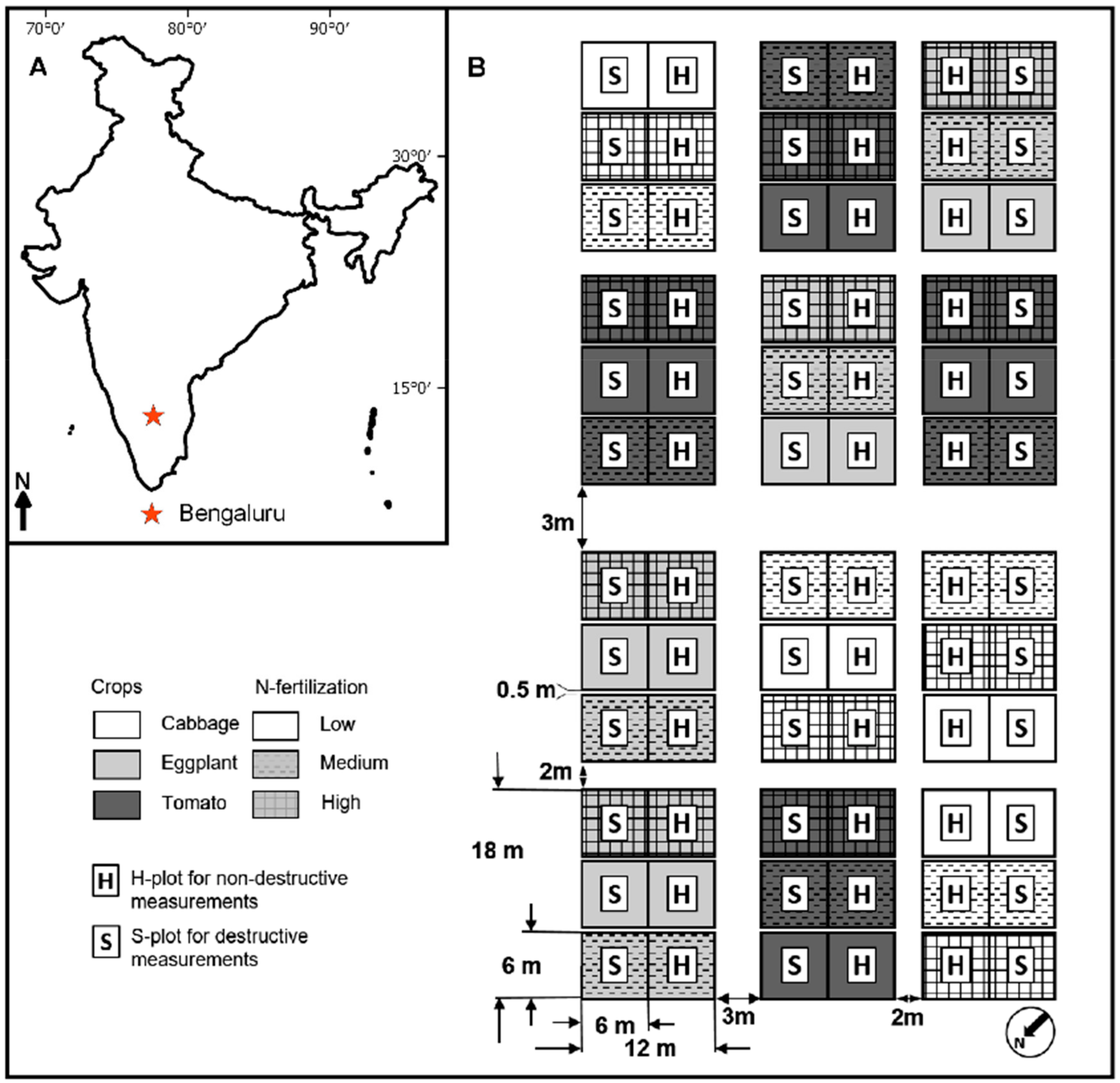
2.1. Study Site
2.2. Experimental Design
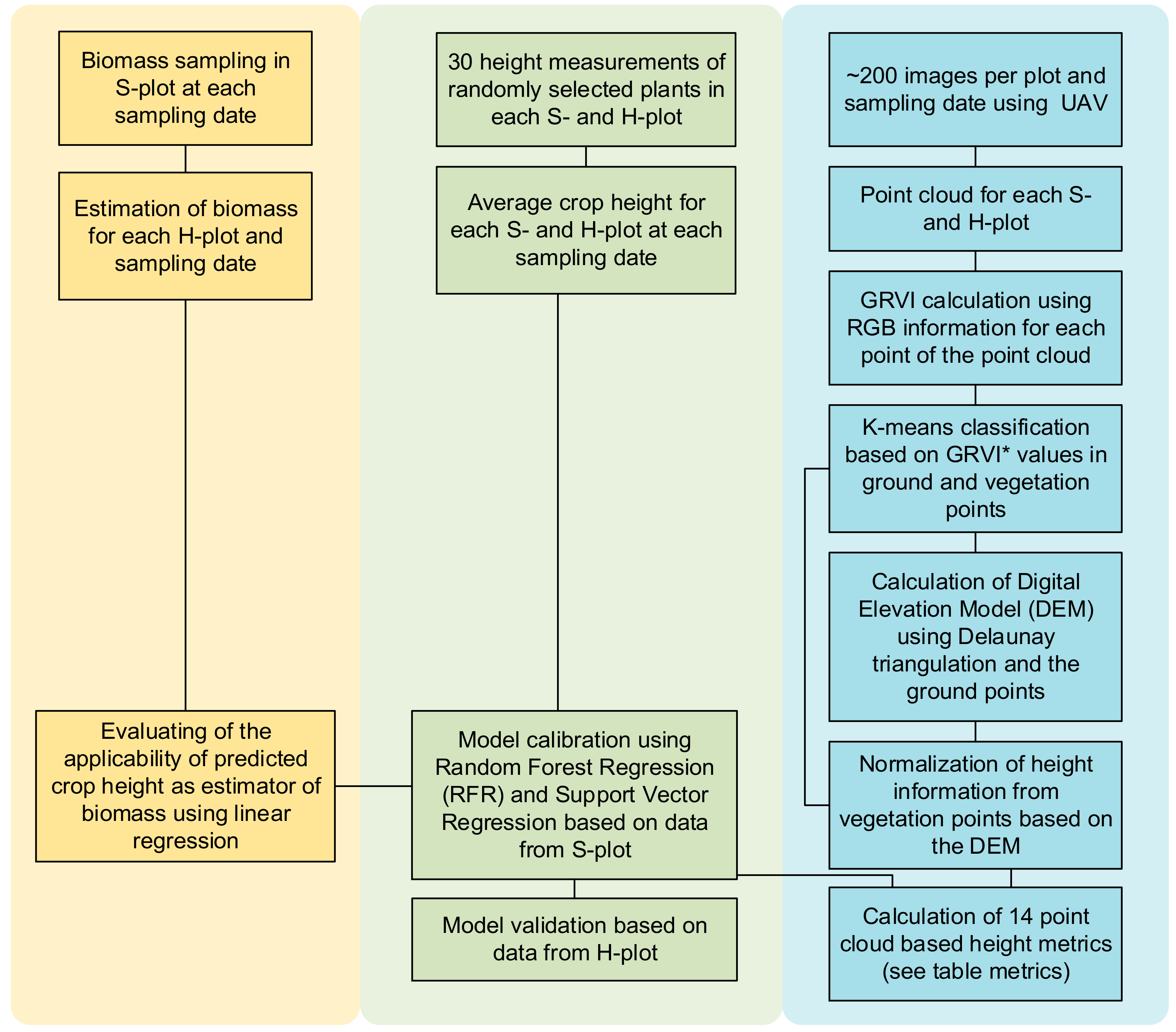
2.3. Plant Sampling and Measurements
2.4. RGB Imagery Sampling
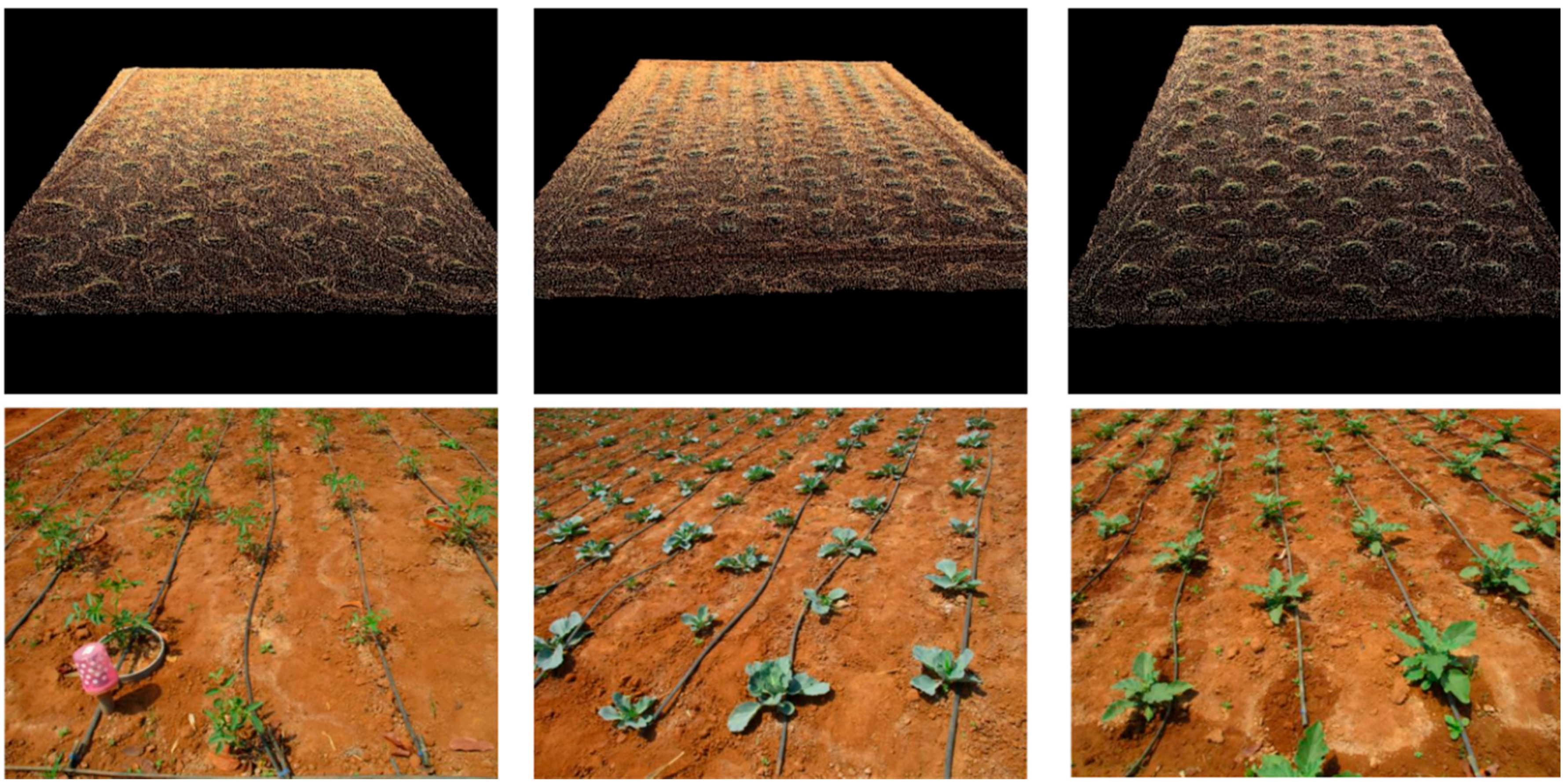
2.5. Point Cloud Processing
2.6. Ground Classification
2.7. Statistical Methods
3. Results
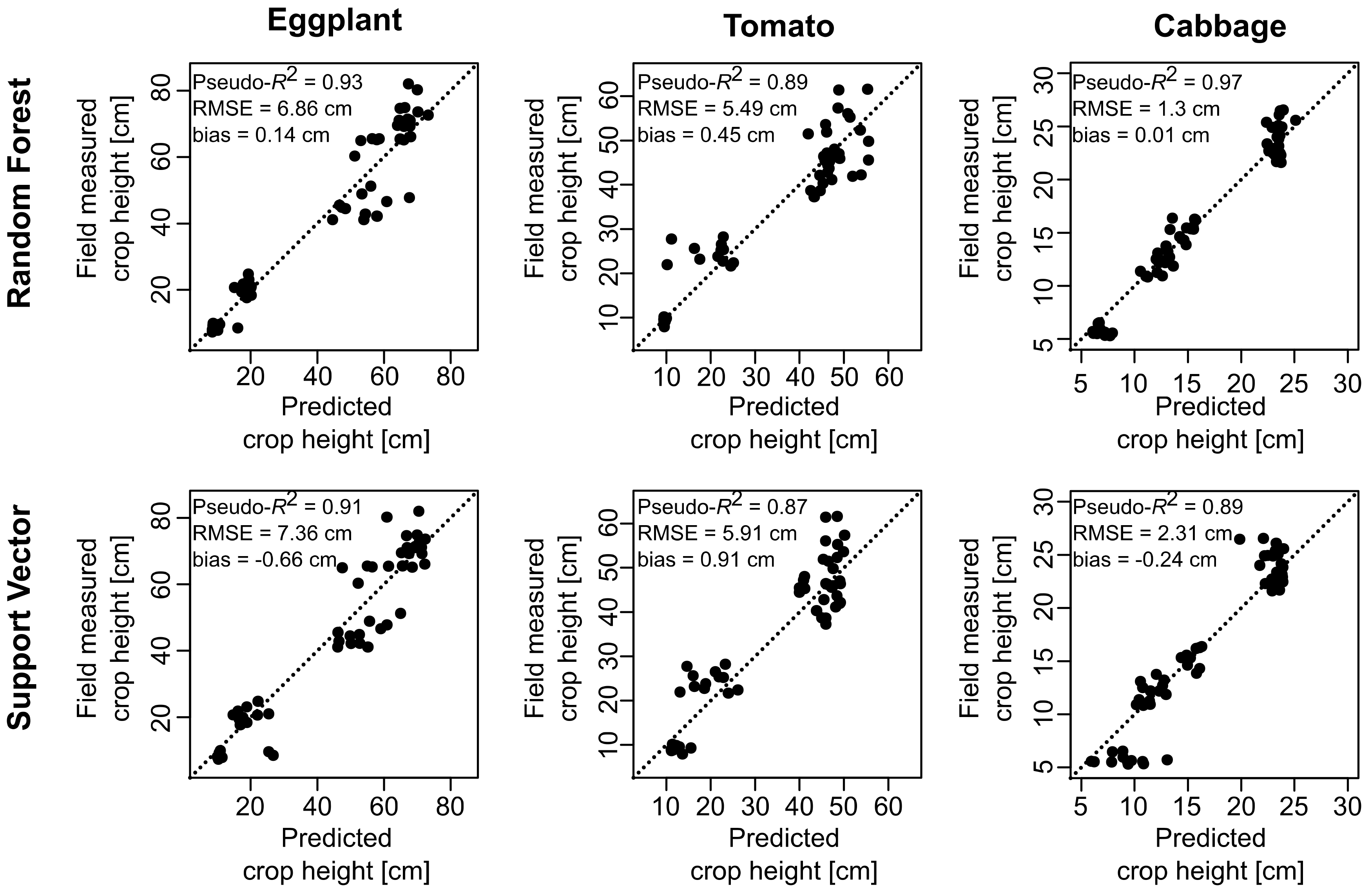
3.1. Crop Height Estimation
3.2. Crop Height Deviation within the Growing Season
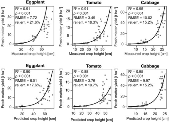
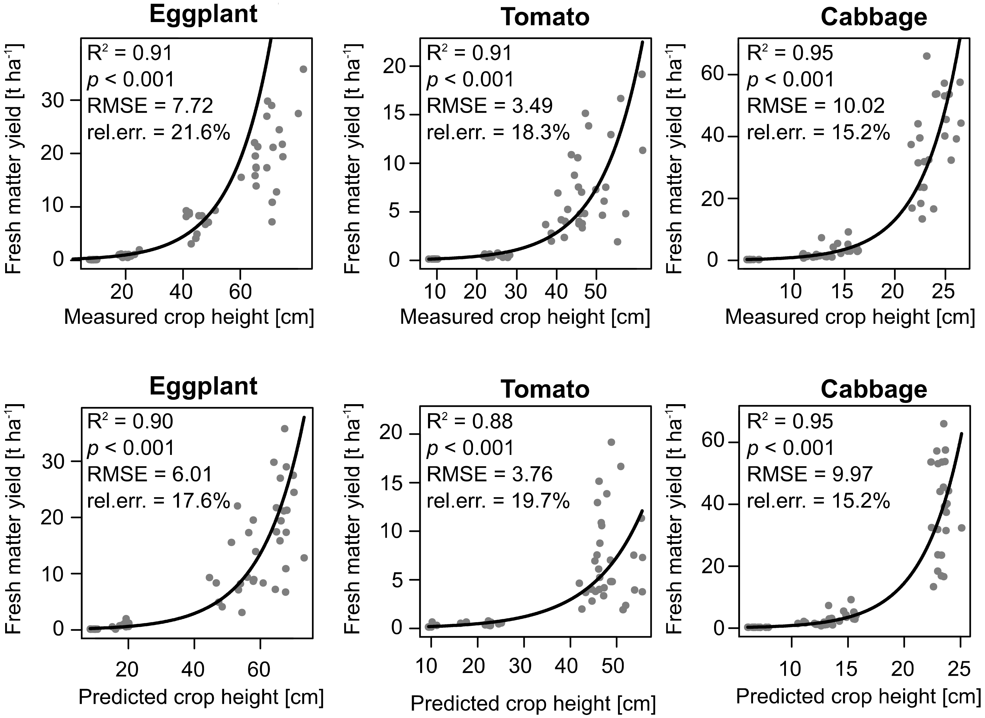
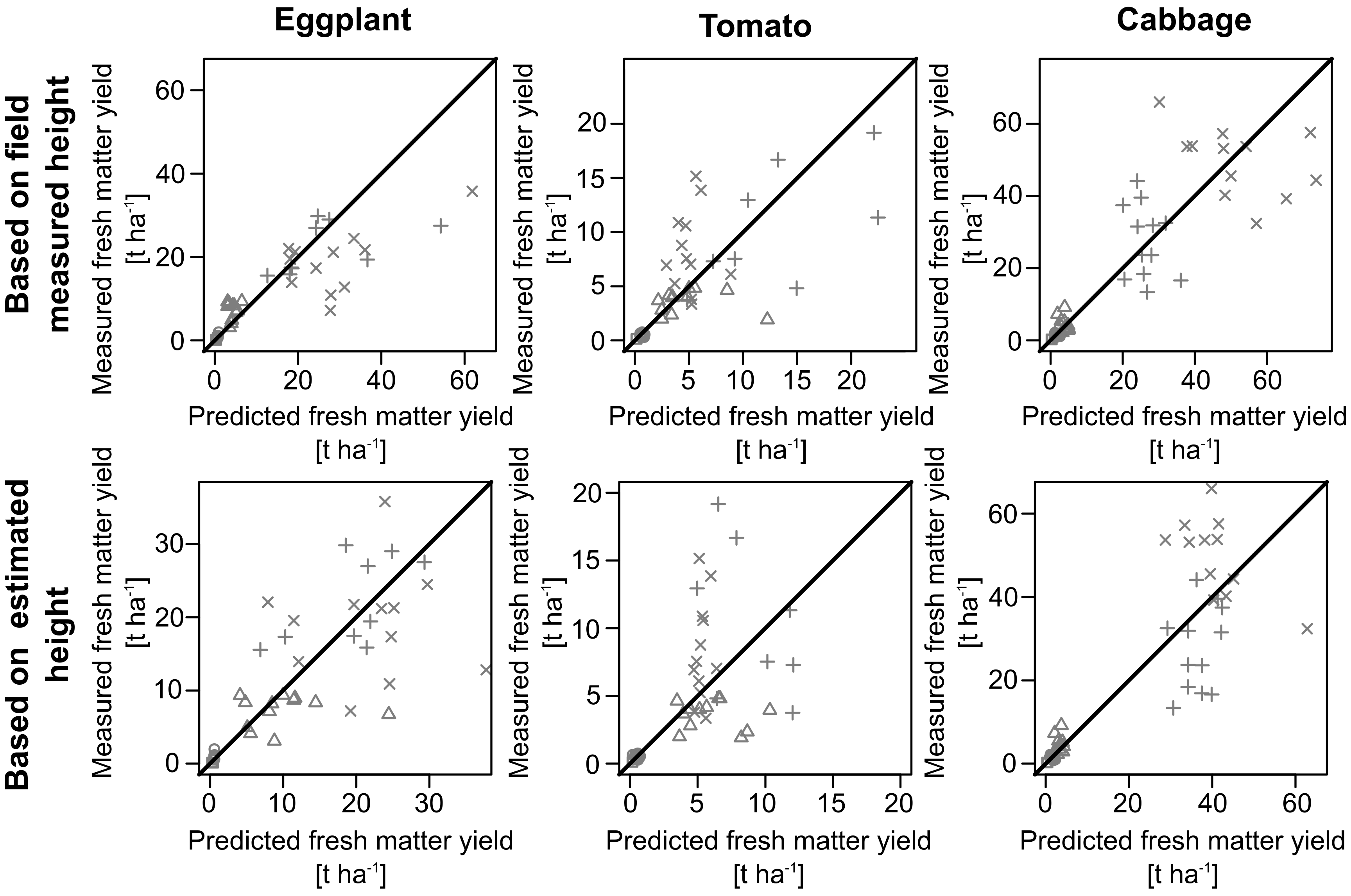
3.3. Crop Biomass Estimation
4. Discussion
5. Uncertainties, Errors, and Accuracies
6. Conclusions
Author Contributions
Acknowledgments
Conflicts of Interest
Appendix A

| Eggplant | Tomato | Cabbage | |
|---|---|---|---|
| Sampling date 1 | 8 March 2017 | 9 March 2017 | 7 March 2017 |
| Sampling date 2 | 29 March 2017 | 30 March 2017 | 28 March 2017 |
| Sampling date 3 | 20 April 2017 | 18 April 2017 | 10 April 2017 |
| Sampling date 4 | 16 May 2017 | 4 May 2017 | 11 May 2017 |
| Sampling date 5 | 13 June 2017 | 5 June 2017 | 7 June 2017 |
| Crop | Sampling Date | Measured Crop Height | Biomass [kg m−2] | Hmin | Hmax | Hmean | Hsd | Hmedian | Hskew | Hkurt | Hcv | Hq70 | Hq80 | Hq90 | Hq95 | Hq99 | Hrelief |
|---|---|---|---|---|---|---|---|---|---|---|---|---|---|---|---|---|---|
| Cabbage | 1 | 5.856 (0.379) | 0.028 (0.028) | 0.001 (0) | 0.173 (0.417) | 0.017 (0.050) | 0.028 (0.107) | 0.005 (0.001) | 3.669 (3.537) | 46.453 (97.946) | 0.989 (0.437) | 0.042 (0.145) | 0.066 (0.248) | 0.081 (0.306) | 0.089 (0.316) | 0.109 (0.329) | 0.099 (0.056) |
| 2 | 11.936 (1.020) | 0.139 (0.139) | 0.001 (0) | 0.168 (0.508) | 0.012 (0.012) | 0.02 (0.057) | 0.007 (0.001) | 1.742 (0.673) | 3.857 (3.906) | 1.005 (0.688) | 0.026 (0.039) | 0.034 (0.056) | 0.051 (0.116) | 0.080 (0.234) | 0.108 (0.328) | 0.132 (0.035) | |
| 3 | 14.947 (1.061) | 0.446 (0.446) | 0.001 (0) | 0.198 (0.446) | 0.017 (0.007) | 0.021 (0.042) | 0.013 (0.001) | 1.685 (1.356) | 6.123 (12.136) | 0.933 (0.737) | 0.035 (0.022) | 0.042 (0.034) | 0.055 (0.063) | 0.075 (0.130) | 0.132 (0.322) | 0.153 (0.052) | |
| 4 | 22.296 (0.892) | 2.746 (2.746) | 0.001 (0) | 0.235 (0.374) | 0.035 (0.005) | 0.032 (0.031) | 0.029 (0.002) | 1.132 (1.417) | 2.738 (12.325) | 0.854 (0.462) | 0.070 (0.016) | 0.080 (0.024) | 0.095 (0.044) | 0.114 (0.086) | 0.177 (0.298) | 0.207 (0.047) | |
| 5 | 24.967 (1.029) | 4.972 (4.972) | 0.001 (0) | 0.320 (0.643) | 0.035 (0.004) | 0.030 (0.022) | 0.029 (0.002) | 1.283 (1.885) | 5.397 (22.835) | 0.825 (0.401) | 0.069 (0.011) | 0.078 (0.015) | 0.093 (0.027) | 0.108 (0.052) | 0.166 (0.233) | 0.186 (0.054) | |
| Eggplant | 1 | 8.744 (0.883) | 0.015 (0.015) | 0.001 (0) | 0.445 (1.299) | 0.006 (0.002) | 0.014 (0.033) | 0.005 (0.001) | 4.546 (6.417) | 75.084 (171.526) | 1.631 (2.860) | 0.011 (0.005) | 0.013 (0.007) | 0.018 (0.016) | 0.021 (0.017) | 0.076 (0.174) | 0.095 (0.056) |
| 2 | 20.020 (1.736) | 0.099 (0.099) | 0.001 (0) | 0.100 (0.013) | 0.018 (0.004) | 0.016 (0.003) | 0.012 (0.003) | 1.321 (0.248) | 1.451 (1.016) | 0.928 (0.067) | 0.038 (0.007) | 0.044 (0.008) | 0.053 (0.009) | 0.060 (0.009) | 0.074 (0.009) | 0.168 (0.030) | |
| 3 | 44.833 (3.433) | 0.727 (0.727) | 0.001 (0) | 0.456 (0.260) | 0.042 (0.004) | 0.034 (0.003) | 0.035 (0.004) | 1.450 (0.493) | 6.031 (9.016) | 0.812 (0.038) | 0.084 (0.008) | 0.095 (0.009) | 0.114 (0.010) | 0.132 (0.010) | 0.176 (0.016) | 0.112 (0.047) | |
| 4 | 68.798 (4.790) | 2.239 (2.239) | 0.001 (0) | 0.326 (0.103) | 0.074 (0.039) | 0.049 (0.015) | 0.066 (0.042) | 0.877 (0.395) | 0.894 (1.329) | 0.719 (0.108) | 0.134 (0.056) | 0.149 (0.058) | 0.171 (0.061) | 0.191 (0.062) | 0.229 (0.063) | 0.226 (0.097) | |
| 5 | 70.315 (4.778) | 1.902 (1.902) | 0.001 (0) | 0.271 (0.042) | 0.054 (0.010) | 0.042 (0.007) | 0.045 (0.009) | 1.100 (0.167) | 1.185 (0.719) | 0.786 (0.036) | 0.107 (0.019) | 0.121 (0.021) | 0.144 (0.024) | 0.164 (0.026) | 0.204 (0.030) | 0.199 (0.033) | |
| Crop | Sampling Date | Measured Crop Height | Biomass [kg m−2] | Hmin | Hmax | Hmean | Hsd | Hmedian | Hskew | Hkurt | Hcv | Hq70 | Hq80 | Hq90 | Hq95 | Hq99 | Hrelief |
| Tomato | 1 | 9.249 (0.592) | 0.014 (0.014) | 0.001 (0) | 0.088 (0.187) | 0.008 (0.011) | 0.011 (0.033) | 0.005 (0) | 2.253 (1.805) | 14.877 (22.386) | 0.833 (0.408) | 0.018 (0.035) | 0.022 (0.046) | 0.035 (0.102) | 0.044 (0.132) | 0.059 (0.162) | 0.129 (0.056) |
| 2 | 24.544 (2.504) | 0.050 (0.050) | 0.001 (0) | 0.131 (0.240) | 0.009 (0.006) | 0.013 (0.025) | 0.006 (0.001) | 2.852 (0.848) | 13.540 (9.779) | 1.079 (0.576) | 0.020 (0.018) | 0.024 (0.026) | 0.037 (0.054) | 0.054 (0.106) | 0.084 (0.169) | 0.091 (0.027) | |
| 3 | 43.651 (4.829) | 0.360 (0.360) | 0.001 (0) | 0.500 (0.534) | 0.033 (0.006) | 0.036 (0.007) | 0.021 (0.006) | 2.880 (4.579) | 69.698 (311.362) | 1.078 (0.128) | 0.076 (0.012) | 0.090 (0.014) | 0.113 (0.020) | 0.137 (0.031) | 0.192 (0.064) | 0.089 (0.030) | |
| 4 | 53.727 (5.782) | 1.140 (1.140) | 0.001 (0) | 0.611 (0.374) | 0.060 (0.030) | 0.061 (0.038) | 0.038 (0.011) | 1.718 (0.403) | 4.884 (3.454) | 0.974 (0.126) | 0.136 (0.080) | 0.160 (0.097) | 0.198 (0.120) | 0.232 (0.137) | 0.306 (0.159) | 0.108 (0.033) | |
| 5 | 46.474 (3.091) | 0.827 (0.827) | 0.001 (0) | 0.305 (0.134) | 0.017 (0.005) | 0.021 (0.010) | 0.010 (0.002) | 4.061 (1.885) | 37.573 (41.772) | 1.220 (0.213) | 0.039 (0.013) | 0.048 (0.018) | 0.065 (0.029) | 0.084 (0.045) | 0.139 (0.075) | 0.060 (0.023) |

References
- Malambo, L.; Popescu, S.C.; Murray, S.C.; Putman, E.; Pugh, N.A.; Horne, D.W.; Richardson, G.; Sheridan, R.; Rooney, W.L.; Avant, R.; et al. Multitemporal field-based plant height estimation using 3D point clouds generated from small unmanned aerial systems high-resolution imagery. Int. J. Appl. Earth Observ. Geoinf. 2018, 64, 31–42. [Google Scholar] [CrossRef]
- Zhang, C.; Kovacs, J.M. The application of small unmanned aerial systems for precision agriculture: A review. Precis. Agric. 2012, 13, 693–712. [Google Scholar] [CrossRef]
- Selsam, P.; Schaeper, W.; Brinkmann, K.; Buerkert, A. Acquisition and automated rectification of high-resolution RGB and near-IR aerial photographs to estimate plant biomass and surface topography in arid agro-ecosystems. Exp. Agric. 2017, 53, 144–157. [Google Scholar] [CrossRef]
- Yu, N.; Li, L.; Schmitz, N.; Tian, L.F.; Greenberg, J.A.; Diers, B.W. Development of methods to improve soybean yield estimation and predict plant maturity with an unmanned aerial vehicle based platform. Remote Sens. Environ. 2016, 187, 91–101. [Google Scholar] [CrossRef]
- Park, S.; Ryu, D.; Fuentes, S.; Chung, H.; Hernández-Montes, E.; O’Connell, M. Adaptive Estimation of Crop Water Stress in Nectarine and Peach Orchards Using High-Resolution Imagery from an Unmanned Aerial Vehicle (UAV). Remote Sens. 2017, 9, 828. [Google Scholar] [CrossRef]
- Johnson, C.K.; Mortensen, D.A.; Wienhold, B.J.; Shanahan, J.F.; Doran, J.W. Site-specific management zones based on soil electrical conductivity in a semiarid cropping system. Agron. J. 2003, 95, 303–315. [Google Scholar] [CrossRef]
- Lati, R.N.; Filin, S.; Eizenberg, H. Estimating plant growth parameters using an energy minimization-based stereovision model. Comput. Electron. Agric. 2013, 98, 260–271. [Google Scholar] [CrossRef]
- Madec, S.; Baret, F.; de Solan, B.; Thomas, S.; Dutartre, D.; Jezequel, S.; Hemmerlé, M.; Colombeau, G.; Comar, A. High-throughput phenotyping of plant height: Comparing unmanned aerial vehicles and ground LiDAR estimates. Front. Plant Sci. 2017, 8, 2002. [Google Scholar] [CrossRef] [PubMed]
- Hoffmeister, D.; Waldhoff, G.; Korres, W.; Curdt, C.; Bareth, G. Crop height variability detection in a single field by multi-temporal terrestrial laser scanning. Precis. Agric. 2016, 17, 296–312. [Google Scholar] [CrossRef]
- Tilly, N.; Hoffmeister, D.; Cao, Q.; Huang, S.; Lenz-Wiedemann, V.; Miao, Y.; Bareth, G. Multitemporal crop surface models: Accurate plant height measurement and biomass estimation with terrestrial laser scanning in paddy rice. J. Appl. Remote Sens. 2014, 8, 083671. [Google Scholar] [CrossRef]
- Fricke, T.; Richter, F.; Wachendorf, M. Assessment of forage mass from grassland swards by height measurement using an ultrasonic sensor. Comput. Electron. Agric. 2011, 79, 142–152. [Google Scholar] [CrossRef]
- Bendig, J.; Bolten, A.; Bennertz, S.; Broscheit, J.; Eichfuss, S.; Bareth, G. Estimating biomass of barley using crop surface models (CSMs) derived from UAV-based RGB imaging. Remote Sens. 2014, 6, 10395–10412. [Google Scholar] [CrossRef]
- Leberl, F.; Irschara, A.; Pock, T.; Meixner, P.; Gruber, M.; Scholz, S.; Wiechert, A. Point clouds. Photogramm. Eng. Remote Sens. 2010, 76, 1123–1134. [Google Scholar] [CrossRef]
- Tumbo, S.D.; Salyani, M.; Whitney, J.D.; Wheaton, T.A.; Miller, W.M. Investigation of laser and ultrasonic ranging sensors for measurements of citrus canopy volume. Appl. Eng. Agric. 2002, 18, 367–372. [Google Scholar] [CrossRef]
- Li, W.; Niu, Z.; Chen, H.; Li, D. Characterizing canopy structural complexity for the estimation of maize LAI based on ALS data and UAV stereo images. Int. J. Remote Sens. 2017, 38, 2106–2116. [Google Scholar] [CrossRef]
- Weiss, M.; Baret, F. Using 3D point clouds derived from UAV RGB imagery to describe vineyard 3D macro-structure. Remote Sens. 2017, 9, 111. [Google Scholar] [CrossRef]
- Schirrmann, M.; Giebel, A.; Gleiniger, F.; Pflanz, M.; Lentschke, J.; Dammer, K.-H. Monitoring agronomic parameters of winter wheat crops with low-cost UAV imagery. Remote Sens. 2016, 8, 706. [Google Scholar] [CrossRef]
- Parkes, S.D.; McCabe, M.F.; Al-Mashhawari, S.K.; Rosas, J. Reproducibility of crop surface maps extracted from Unmanned Aerial Vehicle (UAV) derived Digital Surface Maps. In Remote Sensing for Agriculture, Ecosystems, and Hydrology XVIII; Neale, C.M.U., Maltese, A., Eds.; SPIE: Bellingham, WA, USA, 2016. [Google Scholar]
- Prasad, J.V.N.S.; Rao, C.S.; Srinivas, K.; Jyothi, C.N.; Venkateswarlu, B.; Ramachandrappa, B.K.; Dhanapal, G.N.; Ravichandra, K.; Mishra, P.K. Effect of ten years of reduced tillage and recycling of organic matter on crop yields, soil organic carbon and its fractions in Alfisols of semiarid tropics of southern India. Soil Tillage Res. 2016, 156, 131–139. [Google Scholar] [CrossRef]
- Lowe, D.G. Distinctive image features from scale-invariant keypoints. Int. J. Comput. Vis. 2004, 60, 91–110. [Google Scholar] [CrossRef]
- Snavely, N.; Seitz, S.M.; Szeliski, R. Modeling the world from internet photo collections. Int. J. Comput. Vis. 2008, 80, 189–210. [Google Scholar] [CrossRef]
- Westoby, M.J.; Brasington, J.; Glasser, N.F.; Hambrey, M.J.; Reynolds, J.M. ‘Structure-from-Motion’ photogrammetry: A low-cost, effective tool for geoscience applications. Geomorphology 2012, 179, 300–314. [Google Scholar] [CrossRef] [Green Version]
- Mesas-Carrascosa, F.-J.; Torres-Sánchez, J.; Clavero-Rumbao, I.; García-Ferrer, A.; Peña, J.-M.; Borra-Serrano, I.; López-Granados, F. Assessing optimal flight parameters for generating accurate multispectral orthomosaicks by uav to support site-specific crop management. Remote Sens. 2015, 7, 12793–12814. [Google Scholar] [CrossRef]
- Röder, M.; Hill, S.; Latifi, H. Best Practice Tutorial: Technical Handling of the UAV “DJI Phantom 3 Professional” and Processing of the Acquired Data; Department of Remote Sensing, University of Würzburg: Würzburg, Germany, 2017. [Google Scholar]
- Tucker, C.J. Red and photographic infrared linear combinations for monitoring vegetation. Remote Sens. Environ. 1979, 8, 127–150. [Google Scholar] [CrossRef]
- Motohka, T.; Nasahara, K.N.; Oguma, H.; Tsuchida, S. Applicability of green-red vegetation index for remote sensing of vegetation phenology. Remote Sens. 2010, 2, 2369–2387. [Google Scholar] [CrossRef]
- Silva, C.A.; Hudak, A.T.; Klauberg, C.; Vierling, L.A.; Gonzalez-Benecke, C.; de Padua Chaves Carvalho, S.; Rodriguez, L.C.E.; Cardil, A. Combined effect of pulse density and grid cell size on predicting and mapping aboveground carbon in fast-growing Eucalyptus forest plantation using airborne LiDAR data. Carbon Balance Manag. 2017, 12, 13. [Google Scholar] [CrossRef] [PubMed]
- Næsset, E.; Økland, T. Estimating tree height and tree crown properties using airborne scanning laser in a boreal nature reserve. Remote Sens. Environ. 2002, 79, 105–115. [Google Scholar] [CrossRef]
- Roussel, J.-R.; Auty, D. lidR: Airborne LiDAR Data Manipulation and Visualization for Forestry Applications. Available online: https://CRAN.R-project.org/package=lidR (accessed on 18 May 2018).
- R Core Team. R: A Language and Environment for Statistical Computing; R Core Team: Vienna, Austria, 2016; Available online: https://www.R-project.org/ (accessed on 18 May 2018).
- Breiman, L. Random Forests. Mach. Learn. 2001, 45, 5–32. [Google Scholar] [CrossRef]
- Cortes, C.; Vapnik, V. Support-vector networks. Mach. Learn. 1995, 20, 273–297. [Google Scholar] [CrossRef]
- Liaw, A.; Wiener, M. Classification and Regression by randomForest. R News 2002, 2, 18–22. [Google Scholar]
- Meyer, D.; Dimitriadou, E.; Hornik, K.; Weingessel, A.; Leisch, F. e1071: Misc Functions of the Department of Statistics, Probability Theory Group (Formerly: E1071), TU Wien, 2015. Available online: https://CRAN.R-project.org/package=e1071 (accessed on 18 May 2018).
- Li, W.; Niu, Z.; Chen, H.; Li, D.; Wu, M.; Zhao, W. Remote estimation of canopy height and aboveground biomass of maize using high-resolution stereo images from a low-cost unmanned aerial vehicle system. Ecol. Indic. 2016, 67, 637–648. [Google Scholar] [CrossRef]
- Garcia-Gutierrez, J.; Martínez-Álvarez, F.; Troncoso, A.; Riquelme, J.C. A comparative study of machine learning regression methods on LiDAR data: A case study. In International Joint Conference SOCO’13-CISIS’13-ICEUTE’13; Herrero, Á., Baruque, B., Klett, F., Abraham, A., Snášel, V., de Carvalho, A.C.P.L.F., Bringas, P.G., Zelinka, I., Quintián, H., Corchado, E., Eds.; Springer International Publishing: Cham, Switzerland, 2014; pp. 249–258. [Google Scholar]
- Horning, N. Random forests: An algorithm for image classification and generation of continuous fields data sets. In Proceeding of the International Conference on Geoinformatics for Spatial Infrastructure Development in Earth and Allied Sciences; Hanoi University of Mining and Geology: Hanoi, Vietnam, 2010. [Google Scholar]
- Niederheiser, R.; Rutzinger, M.; Bremer, M.; Wichmann, V. Dense image matching of terrestrial imagery for deriving high-resolution topographic properties of vegetation locations in alpine terrain. Int. J. Appl. Earth Observ. Geoinf. 2018, 66, 146–158. [Google Scholar] [CrossRef]
- Cunliffe, A.M.; Brazier, R.E.; Anderson, K. Ultra-fine grain landscape-scale quantification of dryland vegetation structure with drone-acquired structure-from-motion photogrammetry. Remote Sens. Environ. 2016, 183, 129–143. [Google Scholar] [CrossRef] [Green Version]
- Iqbal, F.; Lucieer, A.; Barry, K.; Wells, R. Poppy Crop Height and Capsule Volume Estimation from a Single UAS Flight. Remote Sens. 2017, 9, 647. [Google Scholar] [CrossRef]
- Bendig, J.; Yu, K.; Aasen, H.; Bolten, A.; Bennertz, S.; Broscheit, J.; Gnyp, M.L.; Bareth, G. Combining UAV-based plant height from crop surface models, visible, and near infrared vegetation indices for biomass monitoring in barley. Int. J. Appl. Earth Observ. Geoinf. 2015, 39, 79–87. [Google Scholar] [CrossRef]
- Moeckel, T.; Safari, H.; Reddersen, B.; Fricke, T.; Wachendorf, M. Fusion of ultrasonic and spectral sensor data for improving the estimation of biomass in grasslands with heterogeneous sward structure. Remote Sens. 2017, 9, 98. [Google Scholar] [CrossRef]
- Safari, H.; Fricke, T.; Reddersen, B.; Moeckel, T.; Wachendorf, M. Comparing mobile and static assessment of biomass in heterogeneous grassland with a multi-sensor system. J. Sens. Sens. Syst. 2016, 5, 301–312. [Google Scholar] [CrossRef]


| Metric | Description |
|---|---|
| Hmin | Minimum crop height |
| Hmax | Maximum crop height |
| Hmean | Mean crop height |
| Hsd | Standard deviation of crop height |
| Hmedian | Median crop height |
| Hskew | Skewness of crop height |
| Hkurt | Kurtosis of crop height |
| Hcv | Coefficient of variation crop height |
| Hq70 | 70th percentile of crop height |
| Hq80 | 80th percentile of crop height |
| Hq90 | 90th percentile of crop height |
| Hq95 | 95th percentile of crop height |
| Hq99 | 99th percentile of crop height |
| Hrelief | Crop canopy relief height (Hmean-Hmin)/(Hmax-Hmin) |
| p-Value | |||
|---|---|---|---|
| Sampling Date (SD) | N Fertilizer (NF) | SD × NF | |
| Eggplant | <0.001 | 0.141 | 0.453 |
| Tomato | <0.001 | 0.978 | 0.720 |
| Cabbage | <0.001 | 0.454 | 0.691 |
| Hmin | Hmax | Hmean | Hsd | Hmedian | Hskew | Hkurt | Hcv | Hq70 | Hq80 | Hq90 | Hq95 | Hq99 | |
|---|---|---|---|---|---|---|---|---|---|---|---|---|---|
| Hmax | 0.01 | ||||||||||||
| Hmean | 0.38 | 0.36 | |||||||||||
| Hsd | 0.1 | 0.67 | 0.75 | ||||||||||
| Hmedian | 0.53 | 0.15 | 0.83 | 0.33 | |||||||||
| Hskew | −0.06 | 0.64 | −0.19 | 0.13 | −0.25 | ||||||||
| Hkurt | −0.02 | 0.55 | −0.08 | 0.07 | -0.09 | 0.84 | |||||||
| Hcv | −0.04 | 0.82 | 0.01 | 0.42 | -0.14 | 0.7 | 0.45 | ||||||
| Hq70 | 0.24 | 0.43 | 0.97 | 0.86 | 0.67 | −0.14 | −0.06 | 0.08 | |||||
| Hq80 | 0.18 | 0.43 | 0.91 | 0.91 | 0.53 | −0.1 | −0.05 | 0.11 | 0.98 | ||||
| Hq90 | 0.15 | 0.49 | 0.86 | 0.95 | 0.45 | −0.05 | −0.04 | 0.19 | 0.95 | 0.98 | |||
| Hq95 | 0.12 | 0.55 | 0.79 | 0.97 | 0.39 | 0.01 | −0.02 | 0.27 | 0.89 | 0.91 | 0.97 | ||
| Hq99 | 0.07 | 0.74 | 0.62 | 0.92 | 0.29 | 0.23 | 0.1 | 0.51 | 0.71 | 0.73 | 0.81 | 0.9 | |
| Hrelief | 0.34 | −0.33 | 0.38 | −0.04 | 0.57 | −0.57 | −0.3 | −0.35 | 0.24 | 0.16 | 0.08 | 0.01 | −0.14 |
© 2018 by the authors. Licensee MDPI, Basel, Switzerland. This article is an open access article distributed under the terms and conditions of the Creative Commons Attribution (CC BY) license (http://creativecommons.org/licenses/by/4.0/).
Share and Cite
Moeckel, T.; Dayananda, S.; Nidamanuri, R.R.; Nautiyal, S.; Hanumaiah, N.; Buerkert, A.; Wachendorf, M. Estimation of Vegetable Crop Parameter by Multi-temporal UAV-Borne Images. Remote Sens. 2018, 10, 805. https://doi.org/10.3390/rs10050805
Moeckel T, Dayananda S, Nidamanuri RR, Nautiyal S, Hanumaiah N, Buerkert A, Wachendorf M. Estimation of Vegetable Crop Parameter by Multi-temporal UAV-Borne Images. Remote Sensing. 2018; 10(5):805. https://doi.org/10.3390/rs10050805
Chicago/Turabian StyleMoeckel, Thomas, Supriya Dayananda, Rama Rao Nidamanuri, Sunil Nautiyal, Nagaraju Hanumaiah, Andreas Buerkert, and Michael Wachendorf. 2018. "Estimation of Vegetable Crop Parameter by Multi-temporal UAV-Borne Images" Remote Sensing 10, no. 5: 805. https://doi.org/10.3390/rs10050805