An Image Fusion Method Based on Image Segmentation for High-Resolution Remotely-Sensed Imagery


1
Key Laboratory of Digital Earth Science, Institute of Remote Sensing and Digital Earth, Chinese Academy of Sciences, No. 9 Dengzhuang South Road, Haidian District, Beijing 100094, China
2
Hainan Key Laboratory Earth Observation, Sanya 572029, China
*
Authors to whom correspondence should be addressed.
Remote Sens. 2018, 10(5), 790; https://doi.org/10.3390/rs10050790
Submission received: 16 April 2018
/
Revised: 16 May 2018
/
Accepted: 17 May 2018
/
Published: 19 May 2018
(This article belongs to the Section Remote Sensing Image Processing)
Abstract
:Fusion of high spatial resolution (HSR) multispectral (MS) and panchromatic (PAN) images has become a research focus with the development of HSR remote sensing technology. In order to reduce the spectral distortions of fused images, current image fusion methods focus on optimizing the approach used to extract spatial details from the PAN band, or on the optimization of the models employed during the injection of spatial details into the MS bands. Due to the resolution difference between the MS and PAN images, there is a large amount of mixed pixels (MPs) existing in the upsampled MS images. The fused versions of these MPs remain mixed, although they may correspond to pure PAN pixels. This is one of the reasons for spectral distortions of fusion products. However, few methods consider spectral distortions introduced by the mixed fused spectra of MPs. In this paper, an image fusion method based on image segmentation was proposed to improve the fused spectra of MPs. The MPs were identified and then fused to be as close as possible to the spectra of pure pixels, in order to reduce spectral distortions caused by fused MPs and improve the quality of fused products. A fusion experiment, using three HSR datasets recorded by WorldView-2, WorldView-3 and GeoEye-1, respectively, was implemented to compare the proposed method with several other state-of-the-art fusion methods, such as haze- and ratio-based (HR), adaptive Gram–Schmidt (GSA) and smoothing filter-based intensity modulation (SFIM). Fused products generated at the original and degraded scales were assessed using several widely-used quantitative quality indexes. Visual inspection was also employed to compare the fused images produced using the original datasets. It was demonstrated that the proposed method offers the lowest spectral distortions and more sharpened boundaries between different image objects than other methods, especially for boundaries between vegetation and non-vegetation objects.
1. Introduction
In recent years, the spatial resolution of remote sensing images has increased greatly and a large number of high-resolution satellites have been launched. High spatial resolution (HSR) remote sensing images contain abundant texture and spatial detail information, which benefits a large amount of remote sensing applications. Thus, the processing of HSR remote sensing images has become a popular research area. Remote sensing image fusion techniques, which can be used to fuse several images provided by one or more sensors covering the same regions to produce high-quality synthesized images, are useful for improving image interpretation and automatic classification. Currently, most of the current HSR satellites provide both an HSR panchromatic (PAN) band and several low spatial resolution (LSR) multispectral (MS) bands. An LSR MS band covers a narrower spectral bandwidth than an HSR PAN band. It is desirable to integrate the geometric details of an HSR PAN band with the LSR MS image to produce an HSR MS image. A large amount of algorithms for MS and PAN image fusion, which is also called pansharpening, has been proposed in the past decades. Concerning the categorization of existing pansharpening methods, it is widely accepted that a majority of current methods can be classified into two major categories: the component substitution (CS) methods and the methods based on multi-resolution analysis (MRA) [1,2,3,4]. Another special categorization is the methods based on PAN-modulation (PM) [5], which provide outstanding fused products with constrained spectral distortions. Some of these methods also belong to the MRA category, such as additive wavelet luminance proportional (AWLP) [6] and additive à trous wavelet transform (ATWT) [7]. In recent years, some model-based methods have been developed [8], using the Bayesian approach [9], sparse representation [10,11,12], compressed sensing [13,14] and the variational model [15,16]. In a recent published book, current pansharpening methods were classified into five groups, including CS, MRA, numerical methods, statistical methods and hybrid methods [17]. Despite most of the current pansharpening methods showing significant differences, the implementation of these methods can be generalized using two steps [18,19]. Firstly, spatial details are extracted from the original PAN band. Then, the extracted spatial details are injected into the upsampled MS bands using different models. Current pansharpening methods employ different approaches to extract spatial details from the PAN band, or different models during the injection of spatial details into the upsampled MS bands. For CS methods, the spatial details, which are obtained by subtracting an intensity component generated by a linear combination of the MS bands from the PAN band, are injected into the upsampled MS bands [18,20]. For MRA methods, spatial details obtained through multiscale decomposition of the PAN band are injected into the upsampled MS bands through additive or multiplicative models. Such models include global models, local models, and context-adaptive models [18,20]. The details of these models can be found in [18,21]. In addition, interpolation approaches for generating upsampled MS bands were discussed in several studies. It was suggested that the bi-cubic interpolation approach should be used to obtain upsampled MS bands, in order to avoid misalignments between expanded MS and PAN bands [22].
As is well known, the mixed pixel (MP) problem is one of the principal sources of errors in remote sensing image interpretation. Generally, the occurrence of the MP problem is due to the fact that a pixel in a remote sensing image covers multiple land cover objects. In the case of two images with different spatial resolutions, the image with a lower spatial resolution contains a larger proportion of MPs than the other [23]. Actually, the MP problem has a serious impact on the quality of fused products. For the fusion of satellite images recorded by multiple sensors, such as Landsat TM/ETM+ and MODIS data fusion, unmixing techniques were employed to produce fusion products [24,25]. Generally, these methods dealt with the case that the HSR image has several spectral bands. For the case where the image with relatively high spatial resolution contained only a single band, some studies also have tried to use unmixing-based methods to produce HSR MS images. The work in [26] discussed fusing a single PAN band with several MS bands with an adaptation of the multiresolution multisensory technique, which is a general method used to fuse images recorded by different sensors with different spatial resolutions. In this method, the HSR PAN image was firstly classified into several classes, and the spectra of every class from the MS images were derived. Finally, the synthetic HSR MS image was generated by assigning the spectra of the corresponding class to each PAN pixel. Although this method proved to be effective for improving the resolution of some image objects, it yielded a relatively poor performance in terms of texture feature enhancement.
In the past few years, the effect of the MP problem on the fusion of MS and PAN images recorded simultaneously by the same platform has been examined by several studies. It was revealed that fused versions of MPs in upsampled MS images remain mixed in the majority of current fusion products, despite some of these MPs perhaps corresponding to pure PAN pixels. This leads to significant differences between the fused spectra of these MPs and those of the corresponding real MS pixels of PAN resolution, if they exist, and contributes to a great amount of spectral distortions and blurred boundaries between different objects existing in fusion products [27]. The work in [28] indicates that most existing fusion methods are based on a pure pixel assumption, and thus, the application of these methods for mixed pixels can lead to incorrect fusion results. The mixed pixels should be unmixed before the fusion process is performed. Two methods based on the linear mixing model and spatial unmixing, respectively, are presented for pansharpening mixed pixels. Moreover, some studies have tried to reduce spectral distortions of fusion products through the improvement of fused spectra of the MPs corresponding to pure PAN pixels. The work in [29] introduced an image fusion method that considers improving the fused spectra of the MPs that correspond to pure PAN pixels, with respect to a classification map obtained by object-oriented classification. In this method, the PAN pixels are roughly classified into several classes, which are mainly related to vegetation and soil, using object-based classification. Then, the MPs are identified and fused to pure pixels, with respect to the class of the corresponding PAN pixels. Although the method proved to be effective for reducing spectral distortion, the performance of this method is highly dependent on classification accuracy. The work in [30] presented an image fusion method based on fusing MPs to pure pixels, using an HSR digital surface model (DSM) derived from airborne light detection and ranging as auxiliary data. Benefiting from the inclusion of an HSR DSM, the PAN pixels were classified into a large number of classes with relatively high classification accuracy. This contributes to the good performance of the method. However, an HSR DSM is rarely available to be used as an auxiliary for the fusion of MS and PAN images, which restricts the use of this method in practice. In addition, only MPs near boundaries between vegetation and non-vegetation objects were considered in this work. The work in [31] proposed an improved fusion method to fuse MPs to pure pixels based on the classification of PAN pixels. It was demonstrated that the fusion products generated by the method can yield more sharpened boundaries and smaller spectral distortions than other products. Similarly, only MPs related to vegetation were considered in this work. Actually, there is also a large number of MPs near boundaries between other image objects. Similarly, some of these MPs may correspond to pure PAN pixels. It is desirable to fuse these MPs to be as close as possible to the spectra of corresponding pure pixels to obtain fusion products with sharpened boundaries and reduced spectral distortions. Thus, an image fusion method based on image segmentation is proposed in this paper to identify more MPs and then improve the fused spectra of these MPs. In this method, MPs near boundaries between different objects are identified with respect to the boundaries of image segments obtained by segmenting the PAN band. The fused spectra of each of the identified MPs are improved with respect to the spectra of a selected pure pixel within the same segment as the MP. A fusion experiment was implemented to evaluate the performance of the proposed method.
This paper is organized as follows. A detailed introduction of the proposed fusion method is presented in Section 2. A fusion experiment used to assess the performance of the proposed method is introduced in Section 3. A discussion of the experimental results is reported in Section 4, and the conclusions are summarized in Section 5.
2. Methodologies
Similar to the method introduced in our previous study [31], MPs are firstly identified, and the fused spectra of each of these MPs are then improved to obtain a fused image with reduced spectral distortions. There are two major differences between this work and the previous work.
Firstly, in the previous work, MPs were identified based on two edge maps obtained from the PAN band and an NDVI map derived from the MS image, respectively. In this work, the MPs are identified and fused with respect to image segments obtained by segmenting the PAN band. Actually, the proposed method is developed under the assumption that pixels within the same segment correspond to the same land cover class. The boundary pixels and their neighbors within the same segment are MPs, whereas the other pixels within the same segment are pure.
Additionally, in our previous studies, an identified MP was fused using the spectra of a pure pixel with the same class as the corresponding PAN pixel, with respect to a classification map for PAN pixels. Although this solution is effective in reducing spectral distortions, it can be observed from the fusion products that these improved MPs are spectrally incontinuous with their neighbors visually. Consequently, a new solution for improving fused spectra of the identified MPs was proposed. In this solution, spectral values of each identified MP were firstly modified according to spectral values of a pure pixel within the same segment as the MP. The fused spectra of each MP were obtained using the modified spectra, to reduce spectral distortions of fusion products.
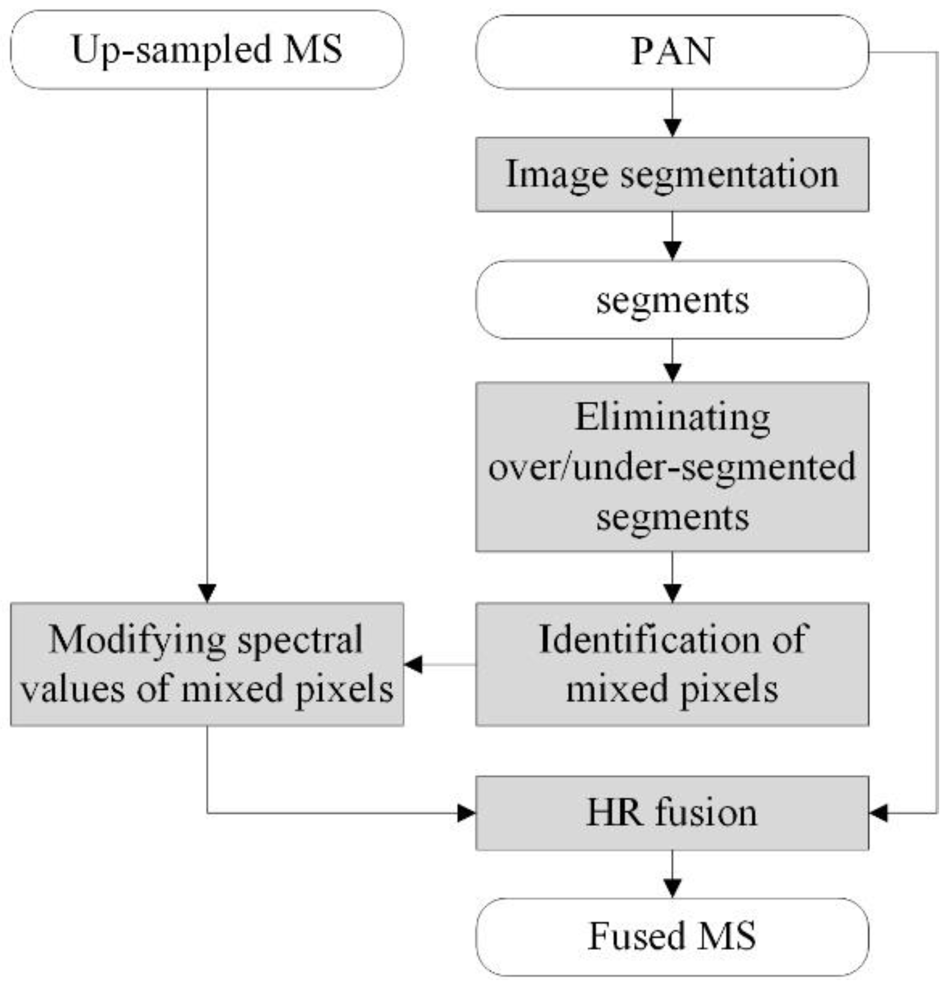
The flowchart of the proposed method is presented in Figure 1. Image segmentation was firstly applied to the PAN band to obtain image segments. The over- and under-segmented segments were then identified and excluded from the following steps. After that, the boundaries of each segment were identified, and pixels near these boundaries were considered as MPs. Then, for each MP, pure pixels within the same segment were located in the neighborhood of the MP, and spectral values of each MP were modified with respect to spectral values of these pure pixels. This yields a modified version of the upsampled MS image. Finally, the original PAN and the modified version of the upsampled MS image were fused to obtain fusion products. The details of each step are introduced in the following sections.
2.1. Image Segmentation
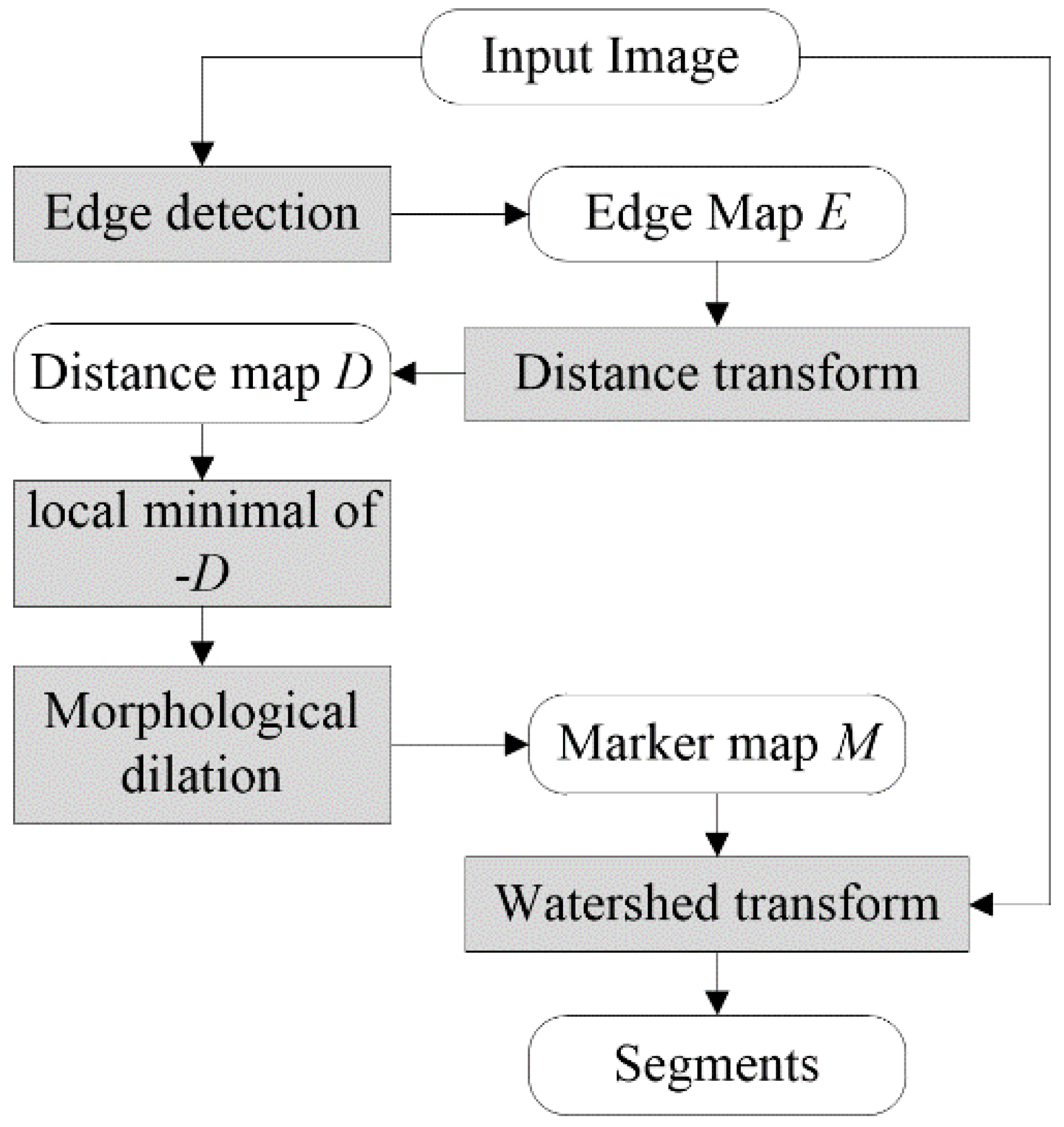
A marker-controlled watershed segmentation method named the edge, mark and fill (EMF) algorithm [32,33] was employed in this work. As MPs are identified and fused regarding segments obtained by segmenting the original PAN band, the accuracy of the employed segmentation algorithm is critical for the proposed fusion method. In order to obtain segments with accurate boundaries, the EMF algorithm, an edge-based watershed segmentation algorithm, was employed. The EMF algorithm performs watershed segmentation with fully-automatic markers generated by applying a series of morphological operations on an edge map [33]. The flow diagram of the EMF algorithms is presented in Figure 2. An edge map E was firstly generated using the Canny edge detector [34], which is well known for its good performance. The Euclidean distance transform was then applied to E to yield a distance map D. After that, a morphological maker M, which is the marker used in the final watershed transform, was yielded based on D, through a marker generation procedure. This procedure consisted of four steps. Firstly, the reciprocal of the distance map D was calculated to generate a distance map -D. Then, the pixels corresponding to local minimums of -D were considered as region seeds. After that, each of these region seeds was dilated with a circular structuring element to generate a basic marker. Finally, all the basic markers were unioned together to generate the final marker map M. Compared with the initial region seeds generated from -D, the marker map M comprised just a few extended markers. This is useful for reducing over-segmented regions, compared with conventional watershed segmentation.
2.2. Elimination of Over- and Under-Segmented Regions
Both under- and over-segmentation have a great effect on the performance of the proposed method. If a segment is over-segmented, some pure pixels may be mistaken as MPs. The modification of spectral values of these pixels may lead to the increase of spectral distortions and the amount of calculation. In contrast, some MPs may be mistaken as pure pixels employed to modify spectral values of identified MPs if some segments are under-segmented. Consequently, both over- and under-segmented segments were identified in this step and then excluded in the following steps.
With respect to some literature about segments’ refinement, such as [35], local intra- and inter-segment heterogeneity statistics were employed in this study to identify over- and under-segmented regions, respectively. For a segment that is under-segmented, it contains two or more types of land cover objects. Normally, this leads to a relatively high variance value of the segment. Thus, under-segmented regions can be identified according to the variances of segments. In this work, a heterogeneity indicator of each segment I, denoted as VRi, was defined with respect to the variance, Vi, and the mean, ui, of the spectral values of segment i, as shown in Equation (1):
This indicator was used as the measure of the intra-segment heterogeneity to identify under-segmented regions. For an over-segmented segment, it should show a high internal homogeneity, as well as a high similarity to its neighbors. As a reliable indicator employed to measure the similarity between a segment and its neighbors, the local Moran’s I (MI) was chosen as the inter-segment heterogeneity indicator to identify over-segmented regions. Local MI, which measures spatial autocorrelation for each segment, was calculated using Equation (2):
where zi, zj are deviations of segments i and j from their mean values, respectively. During the calculation of local MI of each segment, only its neighboring segments were considered. Thus, for the neighbors of segment i, the values of w were one, while for all the other segments, the values of w were zero. In the proposed method, two thresholds were determined to identify under-segmented segments with relative high variances and over-segmented segments with relatively high local MI values, respectively.
2.3. Identification of MPs
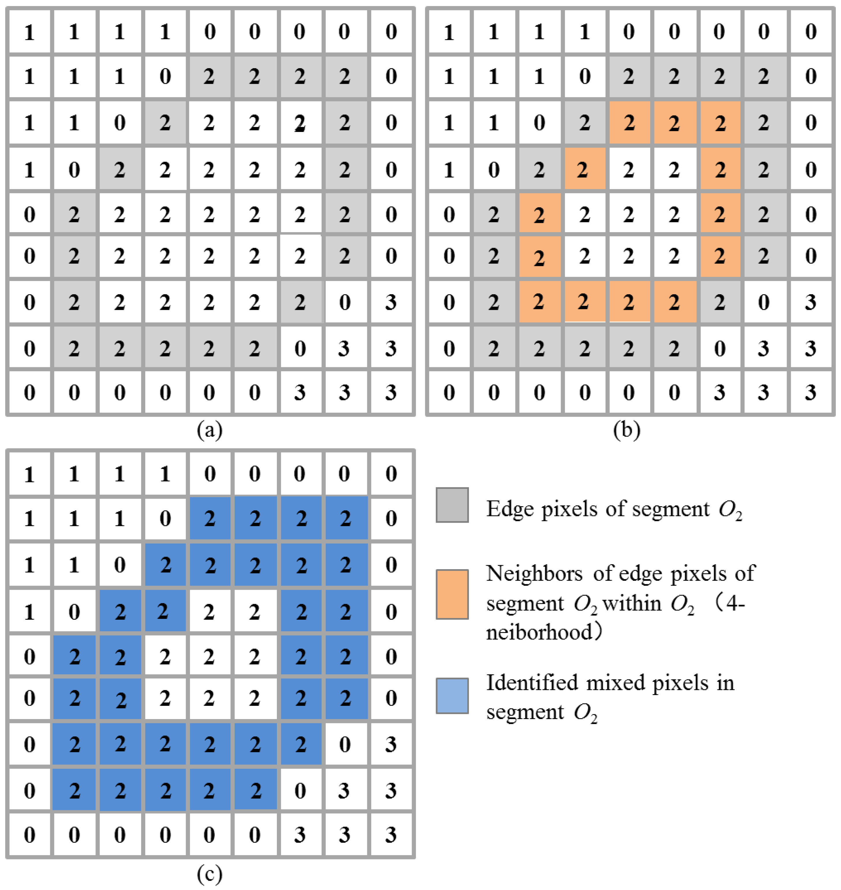
After excluding the under- and over-segmented objects, boundary pixels of each of the remaining segments were identified. These boundary pixels and their neighboring pixels within a certain neighborhood can be taken as MPs. A given segment labeled as i is denoted as Oi, an example for identifying MPs within the segment O2, which is shown in Figure 3. The pixels labeled as zero are edge pixels in the edge map D, as we used an implementation of watershed segmentation as in [36], which does not generate a separate label for edge pixels. The identified boundary pixels of O2 are shown in gray in Figure 3a. Pixels shown in yellow in Figure 3b are the neighboring pixels of each identified boundary pixel within the segment O2. These neighboring pixels of each MP were located using a 4-neighborhood. Finally, the union of the identified boundary pixels and their neighbors, shown in blue in Figure 3c, were taken as MPs in the upsampled MS image.
2.4. Fusion of MPs Using Improved Spectral Values
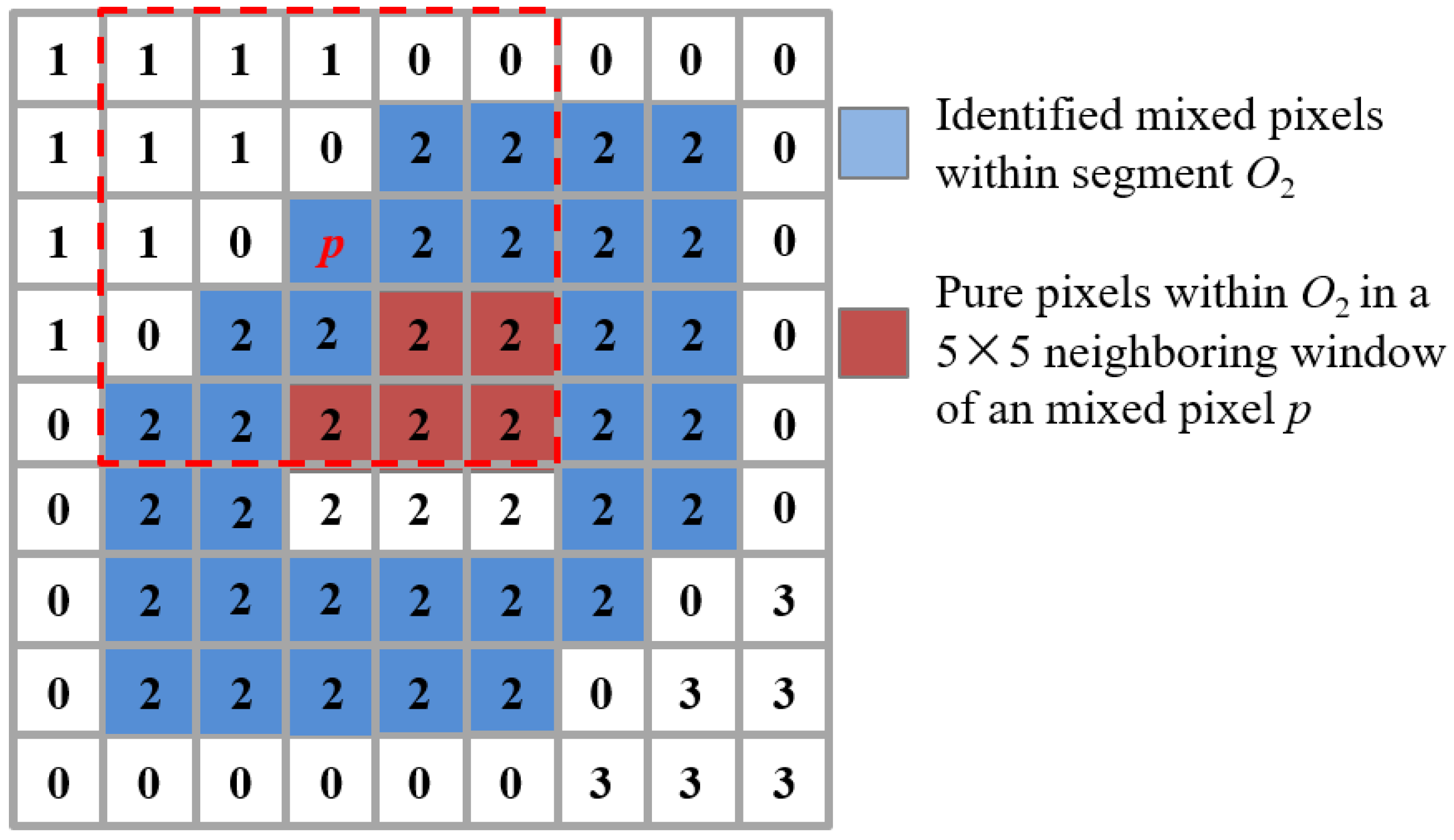
In order to reduce spectral distortion caused by the fused spectra of MPs, the identified MPs were fused using modified spectral values, which were approximate to the spectra of pure pixels within the same segment. Such pure pixels were identified within the same segment as each of the identified MPs, based on the assumption that the pixels within the same segment corresponded to the same land cover class. In addition, these pure pixels were located within a certain neighborhood of each MP. The modified spectra of each MP were then determined with respect to the spectra of these pure pixels. As an example, the location of pure pixels for an identified MP p within the segment O2 is shown in Figure 4. The pixels shown in red in Figure 4 are pure pixels identified within a 5 × 5 local window centered at p. A collection of all these identified pure pixels is denoted as T. The spectra of pixels belonging to T were used to modify the spectra of p. It is obvious that it is hard to find a pure pixel within a segment if the segment is too small. Consequently, only segments with pixels more than a given threshold were considered in this step. For the case using a 5 × 5 neighborhood window to identify a pure pixel, the threshold should be higher than 25 pixels.
Similar to our previous studies, the haze- and ratio-based (HR) fusion method proposed in [37] was employed to produce the final fusion products. The HR method is a PM-based fusion method considering the effect of image haze [38,39,40]. Given that the upsampled MS image is denoted as and the original PAN band is denoted as P, the fused i-th MS band generated by the HR method can be calculated using Equation (3):
where is an assumed low-resolution PAN image, is the i-th upsampled MS band and Hp and Hi are the haze values in the PAN and i-th MS bands, respectively. According to [37], the synthetized low-resolution PAN band was obtained by averaging operation and followed by bi-cubical interpolation to PAN scale. The values of Hi and Hp can be determined using the band minimums of and , respectively [38,39,40]. It can be demonstrated that the fused spectral vector of a pixel is parallel to the corresponding spectral vector in the upsampled MS image [5]. This constrains spectral distortions of fused pixels, especially for pure MS pixels. However, it also leads to the fact that the fused spectral vector of an MP remains mixed, which greatly contributes to spectral distortions occurring in the fusion products.
In order to reduce spectral distortions caused by the mixed fused spectra of MPs, spectral values of each MP in both the upsampled MS image and the synthetized low-resolution PAN band were firstly modified to be more approximate to the spectra of pure pixels within the same segment as the MP. The modified spectra were then used to calculate the fused spectra of an MP. For the MP p shown in Figure 4, the modified spectra of p in the i-th MS band and in the synthetized PAN band can be obtained using Equations (4) and (5), respectively:
In Equation (5), and are the spectra of pure pixels in the i-th MS band and the PAN band, respectively; and α is a weight coefficient. A modified version of the upsampled MS image was produced through the modification of the spectra of each identified MP while retaining the original spectra for the other pixels. Similarity, a modified version of the synthetic low-resolution PAN image was yielded. Finally, the fused i-th MS band was calculated using Equation (6).
The values of and are determined with respect to the spectra of the nearest pure pixel within T from boundary pixels of each segment. A distance map D generated by computing the Euclidean distance transform of a binary image obtained from the segmentation map of the PAN band was employed to find the nearest pure pixels. In the binary image, pixels corresponding to edge pixels in the segmented map were one, whereas the other pixels were zero. For each pixel in the binary image, the distance transform assigned a number that was the distance between the pixel and the nearest nonzero pixel in the binary image. For the MP p, the pure pixel offering the lowest value in D, denoted as q, was identified from the pure pixels in T, i.e., . The values of and were assigned using the spectra of the nearest pure pixel q using Equations (7) and (8), respectively:
The value of is adaptively determined with respect to D(q) and the distance from p to the nearest boundary pixel within the same segment, i.e., D(p), using Equation (9).
3. Experiments
3.1. Datasets
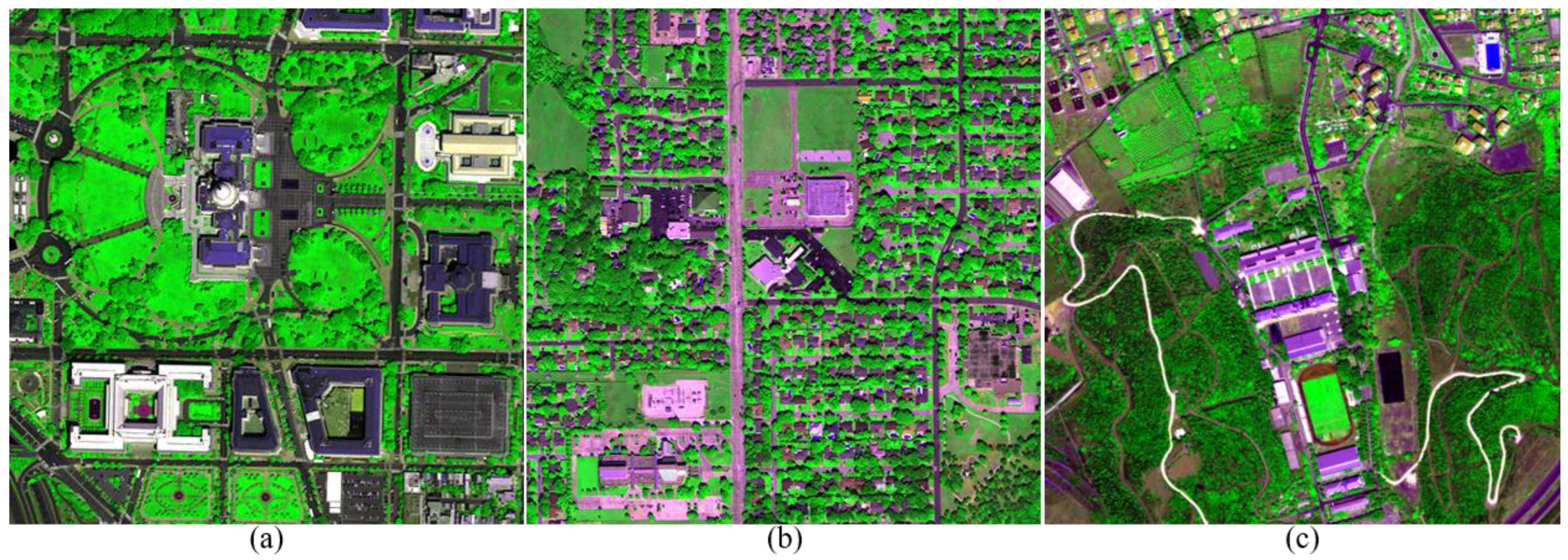
The performance of the proposed method was assessed by a fusion experiment using three datasets acquired by WorldView-2 (WV-2), WorldView-3 (WV-3) and GeoEye-1 (GE-1) satellites, respectively. The WV-2 scene covering Washington DC, USA, was recorded in August 2016. The WV-3 scene covering Dallas, USA, was collected in October 2014. The GE-1 dataset covering Izmir, Turkey, was recorded in September 2014. The MS and PAN images of the WV-2 and WV-3 datasets had resolutions of 1.6 m and 0.4 m, respectively. The PAN image of the GE-1 dataset had a resolution of 0.5 m, whereas the MS image of GE-1 had a resolution of 2 m. For all three datasets, the MS images had a size of 512 × 512 pixels, whereas the PAN images had a size of 2048 × 2048 pixels. The MS images of the WV-2 and WV-3 datasets had eight bands, whereas that of GE-1 had four bands. The MS images for the three datasets are shown in Figure 5. The WV-2 and WV-3 images are shown in compositions of Bands 5, 7 and 2, whereas the GE-1 image is shown in compositions of Bands 3, 4 and 1. It can be seen that typical land cover types, including water-bodies, grasses, trees, buildings, roads and shadows, can be observed in the three images.
Both the degraded and original versions of the three datasets were employed in the experiment. As the quality of fused images is sensitive to misregistration between the MS and PAN bands, we firstly checked the alignments between the original PAN and MS images, using a similar method to the one used in [41]. The degraded MS and PAN images were generated by averaging the pixels within a local window with a size of 4 × 4, as the spatial resolution ratio is for all three datasets [42]. In addition, the upsampled MS bands were produced using a bi-cubic interpolation approach in order to avoid misregistration between the MS and PAN bands [22]. In addition, the alignment between PAN and upsampled MS bands was checked before the fusion experiments.
3.2. Fusion Methods for Comparison and Evaluation Criteria
The proposed method was compared with the original HR method, as well as some outstanding fusion methods widely used in previous studies [43,44,45]. These methods include the adaptive Gram–Schmidt (GSA) method [46], the smoothing filter-based intensity modulation (SFIM) [47,48], the generalized Laplacian pyramid with spectral distortion minimizing model (GLP-SDM) [49], AWLP [6] and ATWT [7]. The GSA and SFIM methods belong to the CS category, whereas the other three methods belong to the MRA category.
The evaluation of these fusion algorithms was performed by both quantitative assessment and visual inspection of the quality of the fusion products. Several commonly-used quality indexes were employed to evaluate the quality of the fusion products of the degraded scale. These indexes include the relative average spectral error (RASE) [50], dimensionless global relative error of synthesis (ERGAS) [51], spectral angle mapper (SAM) [52], a generalization of universal image quality index for monoband images (Q2n) [53,54,55] and the spatial correlation coefficient (SCC) [6]. The quality with no reference (QNR) index was chosen to assess the quality of fused images generated at the original scale [56]. The QNR index is mainly dependent on two separate values, Dλ and DS, which quantify spectral and spatial distortions, respectively [56]. The values of Dλ and DS were reported along with QNR in this work. In terms of visual inspection, subsets of fused images produced at the original scale were presented.
3.3. Results and Analysis
As introduced in Section 2, there are several thresholds that need to be determined during the application of the proposed method. These parameters include a sensitivity threshold for Canny edge detector TC, a threshold for judging under-segmentation based on the relative variances of segments TV, a threshold for judging over-segmentation based on local MI values of segments TM and a threshold used to eliminate small segments TA. The value of TM was set to 0.6 for all the datasets. The values of TA were set to 100 and 30, for the original and degraded datasets, respectively, with respect to the spatial resolutions of the images. The values assigned to the other thresholds TC and TV for each dataset are shown in Table 1, as well as the number of modified MPs, denoted as NMP, by the proposed method. Additionally, NMP values for the case without excluding over- and under-segmented regions and the case that used a TC value automatic determined by the Canny detector are also reported in Table 1. In addition, the proposed method used the same haze values as those used by the HR method. It can be observed that a larger number of MPs are improved in the case that does not exclude under- and over-segmented regions. In contrast, in the case of using automatically determined TC, generally, a smaller number of MPs are improved during the fusion. This is very significant for the GE-1 dataset.
The quality indexes for fused images for the three datasets produced at the two scales are reported in Table 2, in which an expanded MS image generated by upsampling to the PAN scale, without fusion with a PAN band, is denoted as EXP. As the proposed method used the HR method to produce fused images and considered edge information of PAN bands, it is denoted as HR-E in Table 2. The proposed method without excluding over- and under-segmented regions is denoted as HR-E-NE, whereas the proposed method using automatically determined Tc by the Canny detector is denoted as and HR-E-A in Table 2. Additionally, the computation time for each fusion method is also reported in Table 2.
It can be seen that HR-E, HR-E-A and HR-E-NE give similar performances at the original scale, although they offer different values for NMP, as shown in Table 1. Moreover, they offer higher QNR values than the original HR method. For the degraded scale, HR-E and HR-E-A also provide very close Q2n values that are higher than those provided by HR. This indicates that using a Tc value automatically determined by the Canny algorithm is a good choice for the proposed method. In contrast, in the degraded scale, HR-E-NE offers lower Q2n values than HR. This is mainly due to the fact that the fused spectra of some MPs, which are identified from some under-segmented regions obtained using the degraded images, show spectral distortions. Consequently, it can be concluded that under-segmented regions should be excluded from identifying MPs, especially for the fusion of images at the degraded scale, in order to reduce spectral distortion of fused images.
It can be seen from Table 2 that HR-E and HR-E-A offer the highest Q2n values for the degraded WV-2 and WV-3 datasets, followed by the original HR method. The ATWT method provides the highest Q2n values for the degraded GE-1 dataset, followed by the proposed method and HR. The proposed method yields the highest QNR values for the three original datasets, followed by HR. The proposed method provides higher Q2n, SCC and QNR values and lower RASE, ERGAS, SAM and DS values, than the original HR method, for all the three datasets. This indicates that the proposed method, which considers improving the fusion of MPs, is effective at reducing spectral distortions.
Besides HR-E, HR-E-A and HR, the other methods yield slightly different performances for different datasets. For the WV-2 and WV-3 datasets, the GSA method offers higher Q2n and QNR values than SFIM and the three MRA methods, including GLP-SDM, AWLP and ATWT, due to its robustness to aliasing and misregistration errors. The eight bands of WV-2 and WV-3 systems are arranged in two arrays. This acquisition modality can lead to a small temporal misalignment between MS bands [43,57]. The AWLP method gives better performances than ATWT, for the two eight-band datasets and the original GE-1 dataset. This is because AWLP uses the multiplicative injection model, which is proven to be better than the additive injection model used by ATWT [43]. However, for the degraded GE-1 dataset, as an exception, ATWT yields higher Q2n and SCC values and lower SAM and RASE values than the proposed method. This is mainly caused by a very low correlation coefficient (CC) between the PAN and NIR bands of this dataset, resulting in the fact that some vegetation regions are over-enhanced in the fused images generated by the methods using the SDM model, such as HR, AWLP and SFIM. The low CC value between the PAN and NIR bands of this dataset is due to the physics of the satellite, as well as a large amount of vegetation included in this image. For the WV-3 dataset, GLP-SDM offers higher Q2n and QNR values than AWLP and ATWT. For the WV-2 and GE-1 datasets, in contrast, AWLP and ATWT give better performances than GLP-SDM. In addition, it can be observed from Table 2 that the proposed method shows more significant improvements at the original scale than at the degraded scale. This is mainly due to more MPs that are identified and improved by the proposed method at the original scale than at the degraded scale, as shown in Table 1. The computation times for each method used to fuse the original images are also listed in Table 2. All the methods were implemented using MATLAB R2018a. The proposed method uses about 27–43 s to generate a fused product at the original scale. We think the time costs are acceptable as the total times are less than 1 min. The computation time of the proposed method is mainly related to the number of modified MPs, NMP. The image segmentation process requires about 3 s, which is a very short time, whereas a very large percentage of the time is used for identifying MPs and improving their fused spectra.
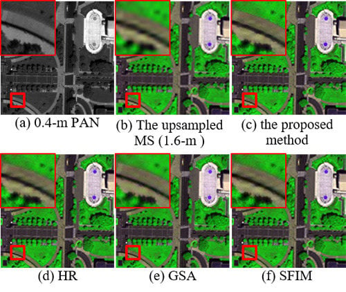
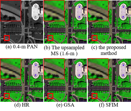
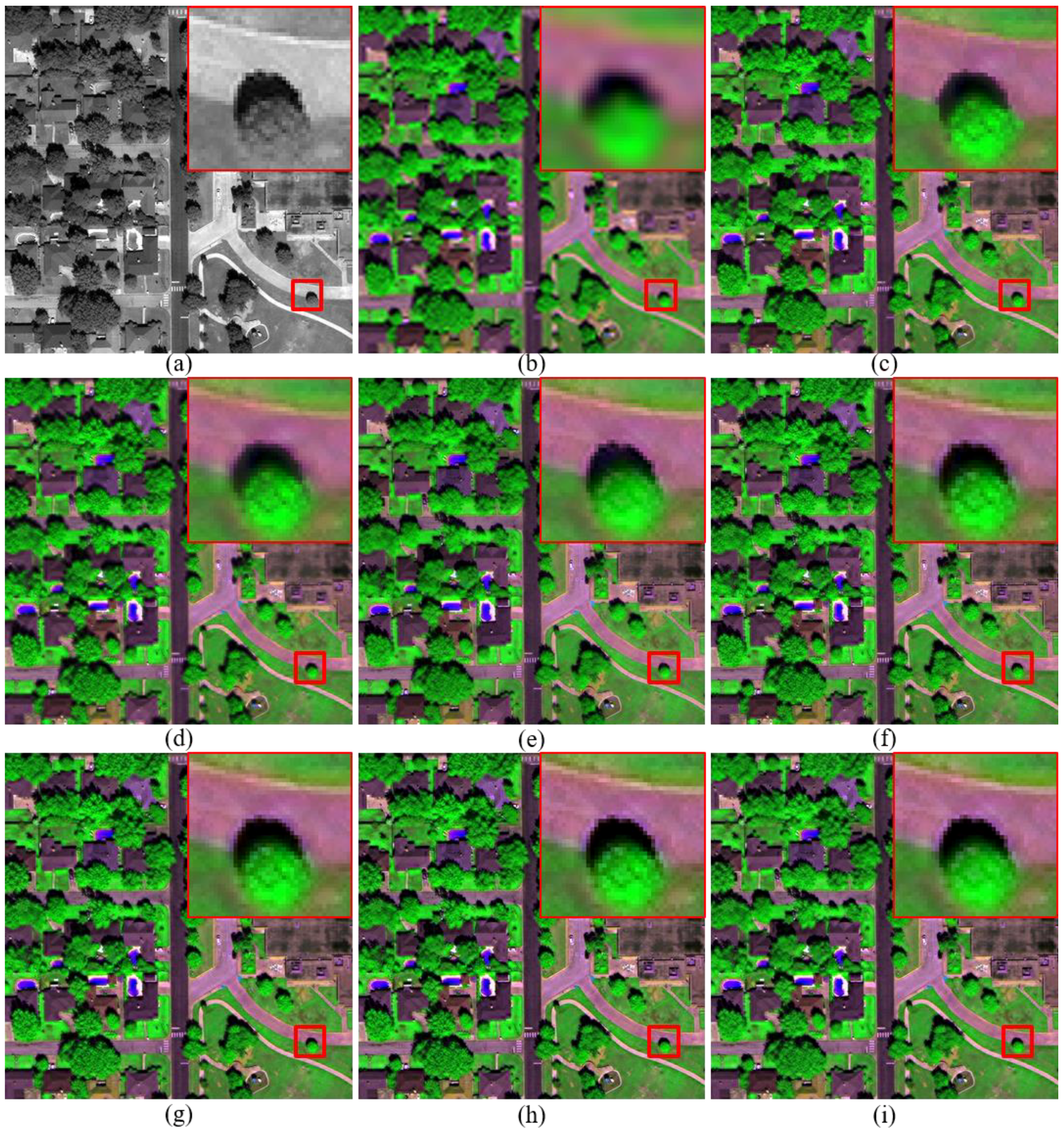
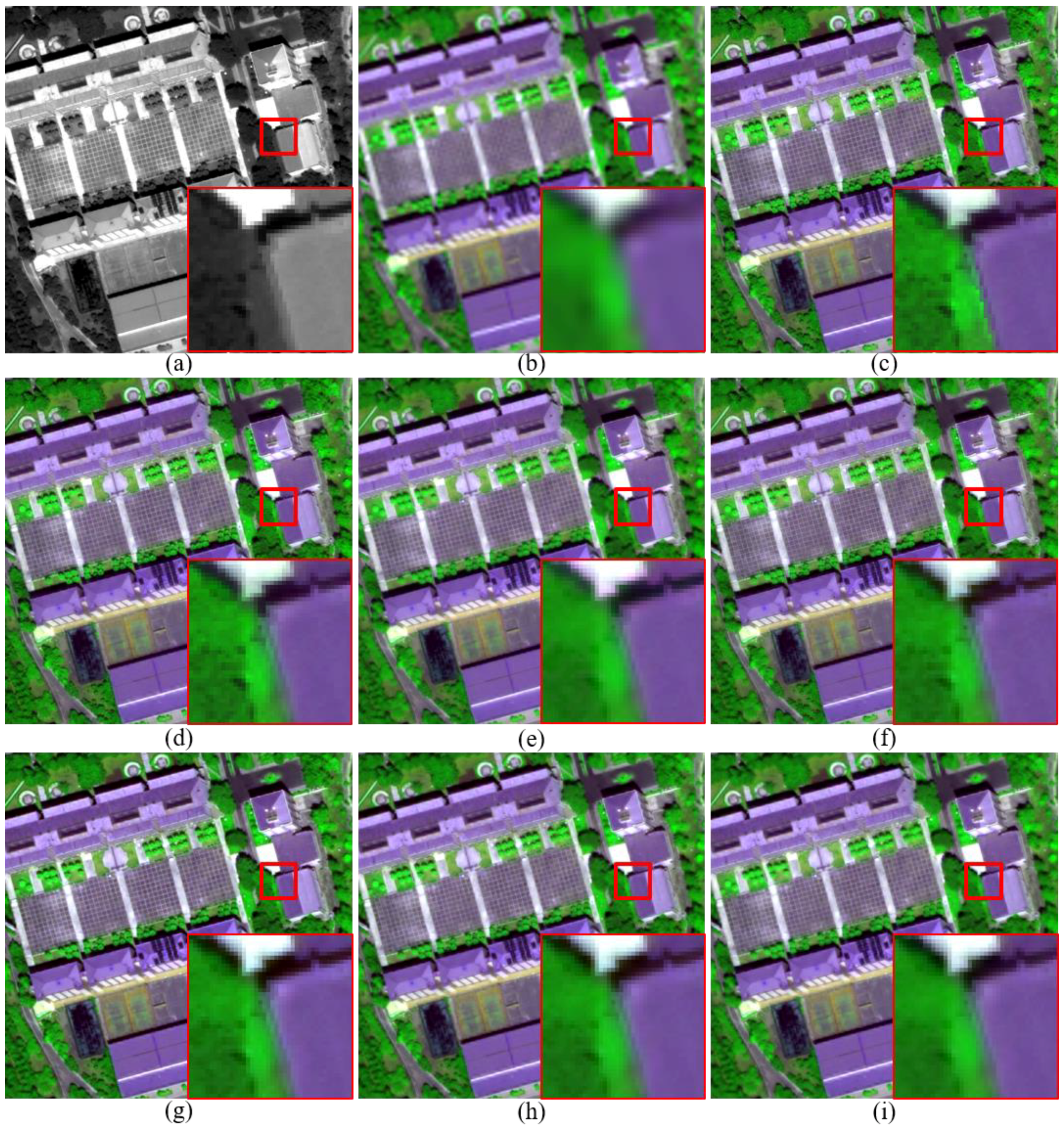
Subsets of the original and fused images of the three datasets at the original scale are shown in Figure 6, Figure 7 and Figure 8, respectively. All the fused MS images are shown after being stretched to the same histogram as the corresponding original MS bands. Each of the subsets has a size of 512 × 512 pixels. The subsets of the WV-2 and WV-3 images are shown in compositions of Bands 5, 7 and 2, whereas those of the GE-1 images are shown in compositions of Bands 3, 4 and 1.
Generally, these fused products show similar visual quality. However, the fused images produced by the improved method show significantly more sharpened boundaries than the others. This is obvious for the fused subsets in red rectangles shown in Figure 6, Figure 7 and Figure 8. It can be observed from Figure 6 that the fused subset produced by the proposed method shows more sharpened boundaries between vegetation areas and roads than the other fused subsets. Similarly, it can be seen that the fused subset generated by the proposed method yields more sharpened boundaries between shadows and roads, as shown in Figure 7, and boundaries between vegetation and buildings, as shown in Figure 8, than the other fusion products. This is also because some MPs near boundaries between different image objects were recognized and fused by the proposed method to be as close as possible to the spectra of corresponding pure pixels. This leads to the fact that the improved fused versions of these MPs show less spectral distortion than the original ones. Actually, there are a large number of MPs near boundaries between different image objects that were recognized, and their fused spectra were improved by the proposed method. The fused spectra of some of these MPs do not show visually noticeable improvements due to the nonsignificant spectral differences between these MPs and the corresponding pure pixels.
Consequently, it can be summarized that the improved approach can reduce spectral distortions of fusion products and sharpen boundaries between different image objects, especially for boundaries between vegetation and other non-vegetation objects.
3.4. Analysis of the Determination of the Thresholds Involved
In this section, experiments were performed to evaluate the robustness of the performance of the proposed method to different thresholds and to provide a reference for selecting the best values for the thresholds involved. A series of fused images was firstly produced by the proposed method using different values assigned to TV, TM and TA, respectively. Then, the quality of these products was evaluated. The three original datasets were used in the experiments.
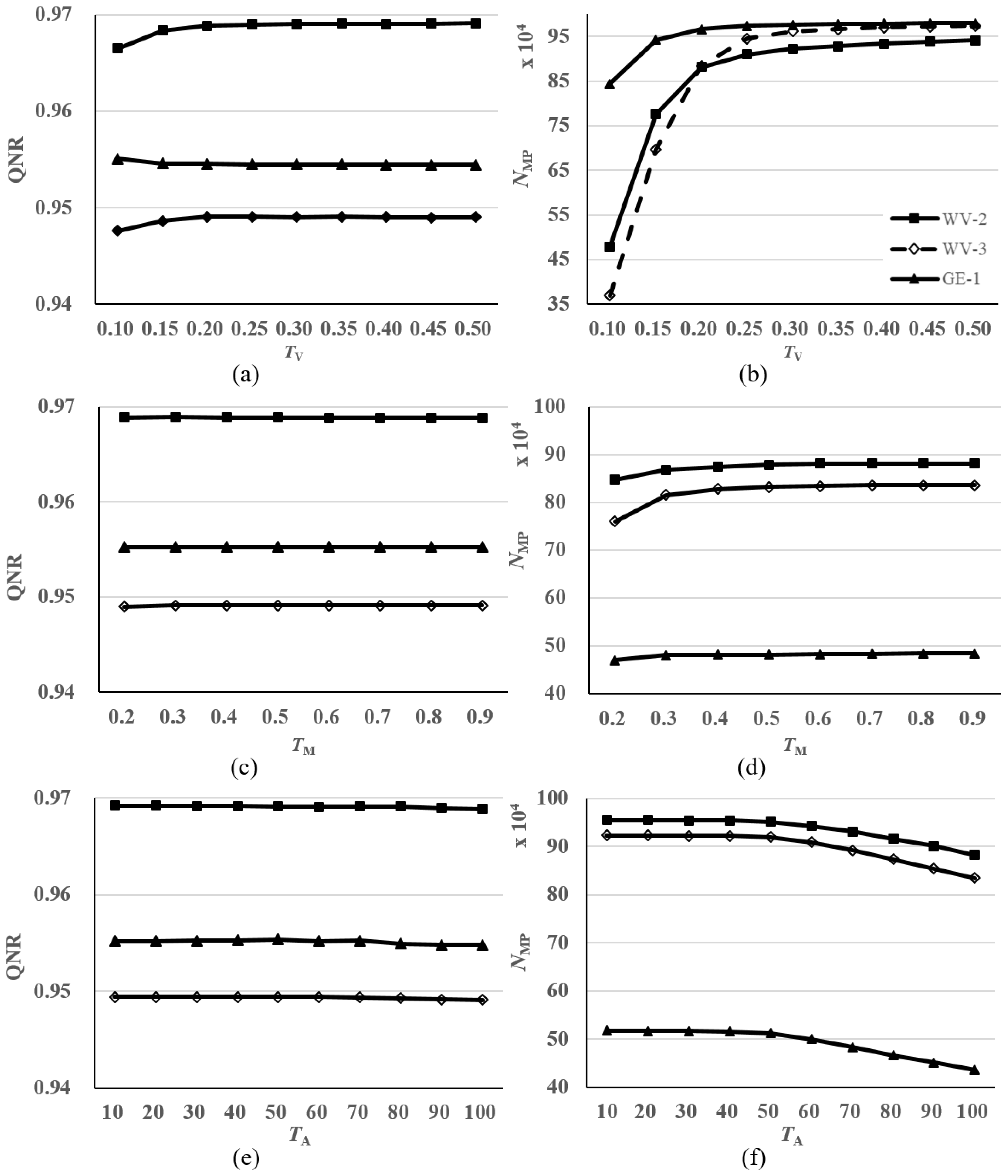
The values assigned to TV, TM and TA are listed in Table 3. In the experiment using different values for TV, the values for TM and TA were set to be the same values as listed in Table 1. Similar approaches were employed during the experiments using different values for TM and TA. The quality of fused images of the three original datasets was assessed using QNR, as shown in Figure 9. The number of modified MPs, NMP, for each product is also shown in Figure 9.
The QNR and NMP for the fused images generated from the three datasets by the proposed method using different values for TV are shown in Figure 9a,b, respectively. Generally, the proposed method offers very close QNR values for each dataset when using TV values higher than 0.2. It can be seen from Figure 9a,b that the proposed method provides the best performances when using TV values between 0.2 and 0.5 for WV-2, between 0.20 and 0.35 for WV-3 and between 0.10 and 0.15 for GE-1. Actually, it is reasonable that the best selection for TV varies from image to image, as relative variances of segments generated from different test images may have different value ranges. A possible solution for selecting an appropriate TV value for a dataset is to determine the value according to the mean and deviation of the relative variances of all the segments.
It can be seen from the QNR and NMP plots shown in Figure 9c,d that neither QNR nor NMP show significant changes when the values for TM vary. Considering the fact that all the segments have values ranging from 0–1, the best selection for TM used by the proposed method may be the median of this range, such as 0.5 and 0.6.
The QNR and NMP for the fused images generated using different values for TA are shown in Figure 9e,f, respectively. Although the value of NMP has an apparent decline along with the increase of TV, the values for QNR are relatively stable. For the WV-2/3 datasets, the values of QNR decrease slowly along with the increase of TA. Generally, TA values ranging from 30–80 are slightly better than the others, for the two datasets. For the GE-1 dataset, QNR yields the highest values when using TA values ranging from 40–50. As introduced in Section 2.4, the value of TA should be higher than 25. It may be concluded that the values ranging from 30–80 are good choices for TA.
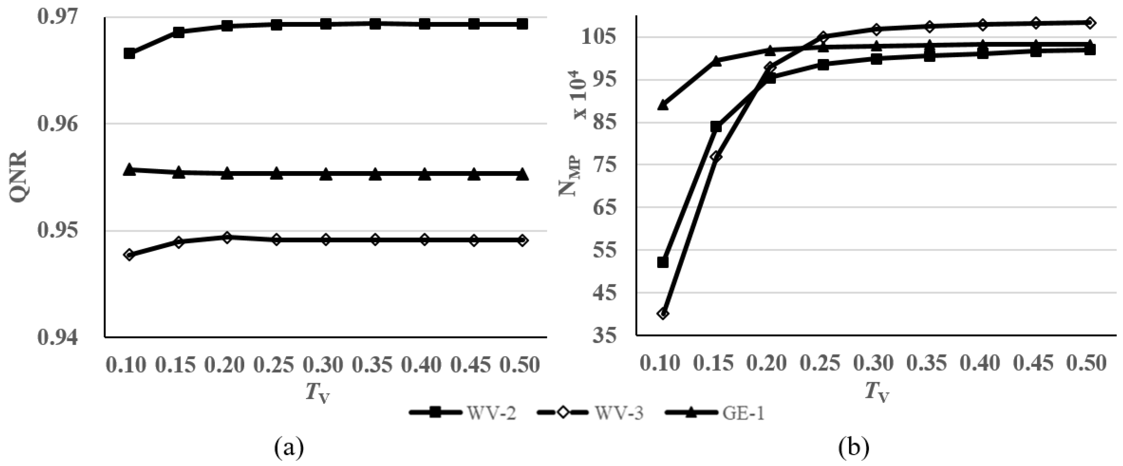
Another experiment was performed to produce fused images by the proposed method using different TV values, with a TA value of 30. The QNR and NMP for the fused images generated from the three datasets using different values for TV are shown in Figure 10a,b, respectively. It can be seen that the curves for the three datasets are very similar to those presented in Figure 9a,b. This indicates that a TA value of 30 is also appropriate for the three datasets.
4. Discussion
The impact of MPs on the quality of fused products of MS and PAN bands simultaneously recorded by the same sensor is rarely considered in current fusion methods. The fused versions of some MPs, which correspond to pure PAN pixels, remain mixed in fused images. We think this is one of the main reasons for the spectral distortions of fusion products, as well as the blurred boundaries between different image objects observed in fused images. The fused spectra of MPs near boundaries between vegetation and non-vegetation objects were improved in previous work. It was demonstrated that reducing spectral distortions that occur in fused versions of MPs is effective in improving the quality of fused products. Different from our previous works, which considered only MPs near boundaries between vegetation and non-vegetation objects, the proposed method in this work takes into account MPs near boundaries between different objects, benefitting from the employment of image segmentation. The proposed method was demonstrated to be effective for reducing spectral distortion and sharpening boundaries between different objects, which is especially noticeable visually for boundaries between vegetation, shadows, water bodies and other image objects.
In the proposed method, MPs are identified based on segments obtained by segmenting the original PAN band. This leads to the fact that the boundary accuracy of each segment has a great impact on the performance of the proposed method. To ensure good and stable performances, image segmentation methods considering edge information are more suitable for the proposed method than other methods not considering edge information, such as the multiresolution image segmentation method in the Ecognition software. In addition, the computing efficiency of the employed image segmentation algorithm is another factor that should be considered. In order to obtain segments with accurate boundaries and ensure a relatively high computational efficiency, the EMF method was employed. It was chosen because it is fast and can obtain segments with accurate boundaries. However, other outstanding image segmentation methods that take into account edge information can also be considered by the proposed method to improve its performance. In addition, boundary pixels in over- and under-segmented regions are not considered in order to avoid introducing spectral distortion and to improve computational efficiency. However, this strategy may limit the number of identified MPs, the fused spectra of which are improved by the proposed method. Further work can also be conducted through refining the over- and under-segmented regions and then including these regions in the following steps to improve the fused spectra of MPs in these regions. Although the proposed method employed the HR method to generate fusion products, similar solutions can be designed and applied to other fusion methods to reduce the spectral distortions caused by MPs. In addition, as MPs are identified and fused according to segments obtained by segmenting the PAN band, the proposed method is sensitive to misalignments between the MS and PAN bands. The alignments between the MS and PAN bands should be checked before the fusion.
The proposed method gave slightly different performances for the three datasets employed in the experiments. This is mainly related to the number of MPs for which the fused spectra are improved, as well as the spatial resolutions and image contexts of the employed datasets. However, the proposed method shows consistent improvements in the experiments using three datasets. Additionally, this solution may be improved in further research. We hold the opinion that the main contribution of this work is that we have provided a novel solution based on image segmentation for reducing spectral distortions existing in pansharpened HSR MS images and sharpening boundaries between different image objects. As boundaries between vegetation, shadows, water bodies and other image objects are significantly sharpened in the fusion products, these kinds of solutions are very useful for generating fusion products used in applications related to vegetation and water bodies.
5. Conclusions
An improved image fusion method based on image segmentation was proposed to reduce spectral distortions of fused images, through the improvement of fused spectra of MPs. In this method, the PAN image was firstly segmented using an edge-based image segmentation method to obtain a large number of image segments. Then, segments that were over- or under-segmented were recognized and excluded in the following steps. After that, boundary pixels of each of the remaining segments were identified, and pixels near these boundaries were then identified as MPs. Next, spectra values of each identified MP were modified according to the spectra of a selected pure pixel within the same segment as the MP. Finally, the identified MPs were fused using the modified spectra, and the other pixels were fused using the original spectra, using the HR method. Using three high-resolution satellite images recorded by WV-2, WV-3 and GE-1, respectively, the proposed method was compared with the GSA, SFIM, GLP, AWLP and ATWT methods. The experimental results show that the fusion products generated by the proposed method yield the smallest spectral distortion, as well as sharpened boundaries between different objects. There are several thresholds that needed to be determined during the application of the proposed method. Experiments were performed to evaluate the robustness of the proposed method and discuss the selection of optimal values for each threshold. It is shown that the performances of the proposed method is relatively stable for different thresholds. Other outstanding image segmentation methods taking into account edge information can be used to take the place of the EMF segmentation used by the proposed method. Although the proposed method employed the HR method to generate fusion products, some other fusion methods can also be used by the proposed method to obtain fused images with less spectral distortions.
Author Contributions
H.L. drafted the manuscript and was responsible for the research design, experiments and the analysis. L.J. provided technical guidance and reviewed the manuscript. Y.T. and L.W. took part in the processing of the GE-1 and WV-3 datasets and reviewed the manuscript.
Acknowledgments
The authors wish to acknowledge two anonymous reviewers for providing helpful suggestions that greatly improved the manuscript. This research was supported in part by the National Key Research and Development Program of China (Grant No. 2017YFC1500902), the Youth Foundation of Director of the Institution of Remote Sensing and Digital Earth, the Chinese Academy of Sciences (Grant No. Y6SJ1100CX), the Key Research Program of the Chinese Academy of Sciences (Grant No. ZDRW-ZS-2016-6-1-3) and the Finance Science and Technology project of Hainan Province, China (Grant No. 418MS113).
Conflicts of Interest
The authors declare no conflict of interest.
References
- Alparone, L.; Wald, L.; Chanussot, J.; Thomas, C.; Gamba, P.; Bruce, L.M. Comparison of pansharpening algorithms: Outcome of the 2006 GRS-S data-fusion contest. IEEE Trans. Geosci. Remote Sens. 2007, 45, 3012–3021. [Google Scholar] [CrossRef] [Green Version]
- Liu, Y.; Chen, X.; Ward, R.K.; Jane Wang, Z. Image fusion with convolutional sparse representation. IEEE Signal Process. Lett. 2016, 23, 1882–1886. [Google Scholar] [CrossRef]
- Aiazzi, B.; Alparone, L.; Baronti, S.; Carla, R.; Garzelli, A.; Santurri, L. Sensitivity of pansharpening methods to temporal and instrumental changes between multispectral and panchromatic data sets. IEEE Trans. Geosci. Remote Sens. 2017, 55, 308–319. [Google Scholar] [CrossRef]
- Li, H.; Jing, L.; Tang, Y.; Ding, H. An improved pansharpening method for misaligned panchromatic and multispectral data. Sensors 2018, 18, 557. [Google Scholar] [CrossRef] [PubMed]
- Aiazzi, B.; Alparone, L.; Baronti, S.; Garzelli, A.; Selva, M. Multispectral pansharpening based on pixel modulation: State of the art and new results. In Proceedings of SPIE, Image and Signal Processing for Remote Sensing XVII; Bruzzone, L., Ed.; SPIE: Bellingham, WA, USA, 2011; Volume 8180, p. 818002. [Google Scholar]
- Otazu, X.; Gonzalez-Audicana, M.; Fors, O.; Nunez, J. Introduction of sensor spectral response into image fusion methods: Application to wavelet-based methods. IEEE Trans. Geosci. Remote Sens. 2005, 43, 2376–2385. [Google Scholar] [CrossRef] [Green Version]
- Shensa, M.J. The discrete wavelet transform: Wedding the a trous and mallat algorithms. IEEE Trans. Signal Process. 1992, 40, 2464–2482. [Google Scholar] [CrossRef]
- Zhang, L.P.; Shen, H.F.; Gong, W.; Zhang, H.Y. Adjustable model-based fusion method for multispectral and panchromatic images. IEEE Trans. Syst. Man Cybern. Part B Cybern. 2012, 42, 1693–1704. [Google Scholar] [CrossRef] [PubMed]
- Zhang, H.K.; Huang, B. A new look at image fusion methods from a bayesian perspective. Remote Sens. 2015, 7, 6828–6861. [Google Scholar] [CrossRef]
- Li, S.; Yin, H.; Fang, L. Remote sensing image fusion via sparse representations over learned dictionaries. IEEE Trans. Geosci. Remote Sens. 2013, 51, 4779–4789. [Google Scholar] [CrossRef]
- Zhu, X.X.; Bamler, R. A sparse image fusion algorithm with application to pan-sharpening. IEEE Trans. Geosci. Remote Sens. 2013, 51, 2827–2836. [Google Scholar] [CrossRef]
- Yin, H. Sparse representation with learned multiscale dictionary for image fusion. Neurocomputing 2015, 148, 600–610. [Google Scholar] [CrossRef]
- Li, S.; Yang, B. A new pan-sharpening method using a compressed sensing technique. IEEE Trans. Geosci. Remote Sens. 2011, 49, 738–746. [Google Scholar] [CrossRef]
- Ghahremani, M.; Ghassemian, H. Remote sensing image fusion using ripplet transform and compressed sensing. IEEE Geosci. Remote Sens. Lett. 2015, 12, 502–506. [Google Scholar] [CrossRef]
- Ma, N.; Zhou, Z.-M.; Zhang, P.; Luo, L.-M. A new variational model for panchromatic and multispectral image fusion. Acta Autom. Sin. 2013, 39, 179–187. [Google Scholar] [CrossRef]
- Zhang, G.; Fang, F.; Zhou, A.; Li, F. Pan-sharpening of multi-spectral images using a new variational model. Int. J. Remote Sens. 2015, 36, 1484–1508. [Google Scholar] [CrossRef]
- Pohl, C.; Van Genderen, J.L. Remote Sensing Image Fusion: A Practical Guide; CRC Press: Boca Raton, FL, USA, 2017. [Google Scholar]
- Aiazzi, B.; Baronti, S.; Lotti, F.; Selva, M. A comparison between global and context-adaptive pansharpening of multispectral images. IEEE Geosci. Remote Sens. Lett. 2009, 6, 302–306. [Google Scholar] [CrossRef]
- Yang, J.; Zhang, J.; Li, H. Generalized model for remotely sensed data pixel-level fusion and its implement technology. J. Image Graph. 2009, 14, 604–614. [Google Scholar]
- Tu, T.-M.; Su, S.-C.; Shyu, H.-C.; Huang, P.S. A new look at IHS-like image fusion methods. Inf. Fusion 2001, 2, 177–186. [Google Scholar] [CrossRef]
- Aiazzi, B.; Alparone, L.; Baronti, S.; Garzelli, A. Context-driven fusion of high spatial and spectral resolution images based on oversampled multiresolution analysis. IEEE Trans. Geosci. Remote Sens. 2002, 40, 2300–2312. [Google Scholar] [CrossRef]
- Aiazzi, B.; Baronti, S.; Selva, M.; Alparone, L. Bi-cubic interpolation for shift-free pan-sharpening. ISPRS J. Photogramm. Remote Sens. 2013, 86, 65–76. [Google Scholar] [CrossRef]
- Schowengerdt, R.A. Remote Sensing, Models and Methods for Image Processing; Academic Press: San Diego and Chesnut Hill, USA, 1997. [Google Scholar]
- Zhukov, B.; Oertel, D.; Lanzl, F.; Reinhackel, G. Unmixing-based multisensor multiresolution image fusion. IEEE Trans. Geosci. Remote Sens. 1999, 37, 1212–1226. [Google Scholar] [CrossRef]
- Gevaert, C.M.; García-Haro, F.J. A comparison of STARFM and an unmixing-based algorithm for Landsat and MODIS data fusion. Remote Sens. Environ. 2015, 156, 34–44. [Google Scholar] [CrossRef]
- Zhukov, B.; Oertel, D.; Lanzl, F. A multiresolution multisensor technique for satellite remote sensing. In Proceedings of the International Geoscience and Remote Sensing Symposium (IGARSS), Firenze, Italy, 10–14 July 1995; Volume 1, pp. 51–53. [Google Scholar]
- Jing, L.; Cheng, Q. Spectral change directions of multispectral subpixels in image fusion. Int. J. Remote Sens. 2011, 32, 1695–1711. [Google Scholar] [CrossRef]
- Palubinskas, G. Model-based view at multi-resolution image fusion methods and quality assessment measures. Int. J. Image Data Fusion 2016, 7, 203–218. [Google Scholar] [CrossRef]
- Jing, L.; Cheng, Q. An image fusion method based on object-oriented classification. Int. J. Remote Sens. 2012, 33, 2434–2450. [Google Scholar] [CrossRef]
- Li, H.; Jing, L.; Wang, L.; Cheng, Q. Improved pansharpening with un-mixing of mixed ms sub-pixels near boundaries between vegetation and non-vegetation objects. Remote Sens. 2016, 8, 83. [Google Scholar] [CrossRef]
- Li, H.; Jing, L.; Sun, Z.; Li, J.; Xu, R.; Tang, Y.; Chen, F. A novel image-fusion method based on the un-mixing of mixed ms sub-pixels regarding high-resolution dsm. Int. J. Digit. Earth 2016, 9, 606–628. [Google Scholar] [CrossRef]
- Gaetano, R.; Masi, G.; Scarpa, G.; Poggi, G. A marker-controlled watershed segmentation: Edge, mark and fill. In Proceedings of the IEEE International Geoscience and Remote Sensing Symposium (IGARSS), Munich, Germany, 22–27 July 2012; pp. 4315–4318. [Google Scholar]
- Gaetano, R.; Masi, G.; Poggi, G.; Verdoliva, L.; Scarpa, G. Marker-controlled watershed-based segmentation of multiresolution remote sensing images. IEEE Trans. Geosci. Remote Sens. 2015, 53, 2987–3005. [Google Scholar] [CrossRef]
- Canny, J. A computational approach to edge detection. IEEE Trans. Pattern Anal. Mach. Intell. 1986, 8, 679–698. [Google Scholar] [CrossRef] [PubMed]
- Johnson, B.; Xie, Z. Unsupervised image segmentation evaluation and refinement using a multi-scale approach. ISPRS J. Photogramm. Remote Sens. 2011, 66, 473–483. [Google Scholar] [CrossRef]
- Bieniek, A.; Moga, A. An efficient watershed algorithm based on connected components. Pattern Recognit. 2000, 33, 907–916. [Google Scholar] [CrossRef]
- Jing, L.; Cheng, Q. Two improvement schemes of pan modulation fusion methods for spectral distortion minimization. Int. J. Remote Sens. 2009, 30, 2119–2131. [Google Scholar] [CrossRef]
- Chavez, P.S. An improved dark-object subtraction technique for atmospheric scattering correction of multispectral data. Remote Sens. Environ. 1988, 24, 459–479. [Google Scholar] [CrossRef]
- Chavez, P.S. Image-based atmospheric corrections revisited and improved. Photogramm. Eng. Remote Sens. 1996, 62, 1025–1036. [Google Scholar]
- Moran, M.S.; Jackson, R.D.; Slater, P.N.; Teillet, P.M. Evaluation of simplified procedures for retrieval of land surface reflectance factors from satellite sensor output. Remote Sens. Environ. 1992, 41, 169–184. [Google Scholar] [CrossRef]
- Li, H.; Jing, L. Improvement of a pansharpening method taking into account haze. IEEE J. Sel. Top. Appl. Earth Obs. Remote Sens. 2017, 10, 5039–5055. [Google Scholar] [CrossRef]
- Jing, L.; Cheng, Q.; Guo, H.; Lin, Q. Image misalignment caused by decimation in image fusion evaluation. Int. J. Remote Sens. 2012, 33, 4967–4981. [Google Scholar] [CrossRef]
- Vivone, G.; Alparone, L.; Chanussot, J.; Dalla Mura, M.; Garzelli, A.; Licciardi, G.A.; Restaino, R.; Wald, L. A critical comparison among pansharpening algorithms. IEEE Trans. Geosci. Remote Sens. 2015, 33, 2565–2586. [Google Scholar] [CrossRef]
- Yin, H.; Li, S. Pansharpening with multiscale normalized nonlocal means filter: A two-step approach. IEEE Trans. Geosci. Remote Sens. 2015, 53, 5734–5745. [Google Scholar]
- Hallabia, H.; Kallel, A.; Hamida, A.B.; Hégarat-Mascle, S.L. High spectral quality pansharpening approach based on MTF-matched filter banks. Multidimens. Syst. Signal Process. 2016, 27, 831–861. [Google Scholar] [CrossRef]
- Aiazzi, B.; Baronti, S.; Selva, M. Improving component substitution pansharpening through multivariate regression of MS + PAN data. IEEE Trans. Geosci. Remote Sens. 2007, 45, 3230–3239. [Google Scholar] [CrossRef]
- Liu, J.G. Smoothing filter-based intensity modulation: A spectral preserve image fusion technique for improving spatial details. Int. J. Remote Sens. 2000, 21, 3461–3472. [Google Scholar] [CrossRef]
- Wald, L.; Ranchin, T. Liu ‘Smoothing filter-based intensity modulation: A spectral preserve image fusion technique for improving spatial details’. Int. J. Remote Sens. 2002, 23, 593–597. [Google Scholar] [CrossRef]
- Aiazzi, B.; Alparone, L.; Baronti, S.; Garzelli, A. MTF-tailored multiscale fusion of high-resolution MS and Pan imagery. Photogramm. Eng. Remote Sens. 2006, 72, 591–596. [Google Scholar] [CrossRef]
- Ranchin, T.; Wald, L. Fusion of high spatial and spectral resolution images: The ARSIS concept and its implementation. Photogramm. Eng. Remote Sens. 2000, 66, 49–61. [Google Scholar]
- Wald, L. Quality of high resolution synthesised images: Is there a simple criterion? In Proceedings of the International Conference on Fusion Earth Data, Sophia Antipolis, France, 26–28 January 2000; pp. 99–103. [Google Scholar]
- Yuhas, R.; Goetz, A.; Boardman, J. Discrimination among semi-arid landscape endmembers using the spectral angle mapper (SAM) algorithm. In Proceedings of the Summaries of the Third Annual JPL Airborne Geoscience Workshop, Pasadena, CA, USA, 15 June 1992; pp. 147–149. [Google Scholar]
- Wang, Z.; Bovik, A.C. A universal image quality index. IEEE Signal Process. Lett. 2002, 9, 81–84. [Google Scholar] [CrossRef]
- Alparone, L.; Baronti, S.; Garzelli, A.; Nencini, F. A global quality measurement of pan-sharpened multispectral imagery. IEEE Geosci. Remote Sens. Lett. 2004, 1, 313–317. [Google Scholar] [CrossRef]
- Garzelli, A.; Nencini, F. Hypercomplex quality assessment of multi/hyperspectral images. IEEE Geosci. Remote Sens. Lett. 2009, 6, 662–665. [Google Scholar] [CrossRef]
- Alparone, L.; Alazzi, B.; Baronti, S.; Garzelli, A.; Nencini, F.; Selva, M. Multispectral and panchromatic data fusion assessment without reference. Photogramm. Eng. Remote Sens. 2008, 74, 193–200. [Google Scholar] [CrossRef]
- Updike, T.; Comp, C. Radiometric Use of Worldview-2 Imagery; Digital Globe: Longmont, CO, USA, 2010. [Google Scholar]
Figure 1.
The flow diagram for the proposed method. MS, multispectral.

Figure 2.
Flowchart of the edge, mark and fill (EMF) segmentation.

Figure 3.
The procedure of the identification of mixed pixels (MPs) within a segment. (a) edge pixels (in gray) of a segment. (b) neighbors (in orange) of the edge pixels shown in (a) within the same segment. (c) identified mixed pixels (in blue) in the segment.
Figure 3.
The procedure of the identification of mixed pixels (MPs) within a segment. (a) edge pixels (in gray) of a segment. (b) neighbors (in orange) of the edge pixels shown in (a) within the same segment. (c) identified mixed pixels (in blue) in the segment.

Figure 4.
Identification of pure pixels in the neighborhood of an MP p within the segment O2.

Figure 5.
The MS images of the three datasets used in the experiment; (a) WV-2 dataset; (b) WV-3 dataset; and (c) GE-1 dataset.
Figure 5.
The MS images of the three datasets used in the experiment; (a) WV-2 dataset; (b) WV-3 dataset; and (c) GE-1 dataset.

Figure 6.
The original and fused images for a 512 × 512 subset of the original WV-2 dataset; (a) 0.4-m PAN; (b) the upsampled version of 1.6-m MS; and fused images generated by the (c) HR-E, (d) HR, (e) GSA, (f) SFIM, (g) GLP-SDM, (h) AWLP and (i) ATWT methods.
Figure 6.
The original and fused images for a 512 × 512 subset of the original WV-2 dataset; (a) 0.4-m PAN; (b) the upsampled version of 1.6-m MS; and fused images generated by the (c) HR-E, (d) HR, (e) GSA, (f) SFIM, (g) GLP-SDM, (h) AWLP and (i) ATWT methods.

Figure 7.
The original and fused images for a 512 × 512 subset of the original WV-3 dataset; (a) 0.4-m PAN; (b) the upsampled version of 1.6-m MS; and fused images generated by the (c) HR-E, (d) HR, (e) GSA, (f) SFIM, (g) GLP-SDM, (h) AWLP and (i) ATWT methods.
Figure 7.
The original and fused images for a 512 × 512 subset of the original WV-3 dataset; (a) 0.4-m PAN; (b) the upsampled version of 1.6-m MS; and fused images generated by the (c) HR-E, (d) HR, (e) GSA, (f) SFIM, (g) GLP-SDM, (h) AWLP and (i) ATWT methods.

Figure 8.
The original and fused images for a 512 × 512 subset of the original GE-1 dataset; (a) 0.5-m PAN; (b) the upsampled version of 2-m MS; and fused images generated by the (c) HR-E, (d) HR, (e) GSA, (f) SFIM, (g) GLP-SDM, (h) AWLP and (i) ATWT methods.
Figure 8.
The original and fused images for a 512 × 512 subset of the original GE-1 dataset; (a) 0.5-m PAN; (b) the upsampled version of 2-m MS; and fused images generated by the (c) HR-E, (d) HR, (e) GSA, (f) SFIM, (g) GLP-SDM, (h) AWLP and (i) ATWT methods.

Figure 9.
The QNR and NMP of fused images for the three original datasets generated by the proposed method using different TV, TM and TA values. (a) QNR and (b) NMP of fused images of the proposed method using TV values ranging between 0.1 and 0.5 with a step of 0.05; (c) QNR and (d) NMP of fused images of the proposed method using TM values ranging between 0.2 and 0.9 with a step of 0.1; (e) QNR and (f) NMP of fused images of the proposed method using TA values ranging from 10–100 with a step of 10.

Figure 10.
The QNR (a) and NMP (b) of fused images for the three datasets generated using different TV values, with a TA value of 30.
Figure 10.
The QNR (a) and NMP (b) of fused images for the three datasets generated using different TV values, with a TA value of 30.


Table 1.
The thresholds used by the proposed method to produce fused images of the three datasets.
| Dataset | Scale | TC | TV | NMP | NMP (without Excluding Some Regions) | NMP (Using Automatic Determined TC) |
|---|---|---|---|---|---|---|
| WV-2 | degraded | 0.07 | 0.1 | 25,700 | 90,286 | 10,709 |
| original | 0.07 | 0.2 | 895,243 | 954,407 | 881,755 | |
| WV-3 | degraded | 0.08 | 0.07 | 10,740 | 92,320 | 5110 |
| original | 0.08 | 0.18 | 825,574 | 980,506 | 834,269 | |
| GE-1 | degraded | 0.09 | 0.07 | 21,152 | 76,162 | 16,686 |
| original | 0.06 | 0.065 | 748,213 | 1,063,620 | 482,849 |
Table 2.
Quality indices of fused images for the datasets used in the experiment. RASE, relative average spectral error; ERGAS, global relative error of synthesis; SAM, spectral angle mapper; Q2n, a generalization of universal image quality index for monoband images; SCC, spatial correlation coefficient; QNR, quality with no reference; GSA, adaptive Gram–Schmidt; SFIM, smoothing filter-based intensity modulation; GLP-SDM, generalized Laplacian pyramid with spectral distortion minimizing model; AWLP, additive wavelet luminance proportional; ATWT, à trous wavelet transform; HR-E, the proposed method; HR-E-A, the proposed method using automatic Canny threshold; HR-E-NE, the proposed method without excluding over- and under-segmented regions; EXP, expanded.
| Image | Method | Degraded Scale | Original Scale | |||||||
|---|---|---|---|---|---|---|---|---|---|---|
| RASE | ERGAS | SAM | Q2n | SCC | Dλ | DS | QNR | Time(s) | ||
| WV-2 | HR-E | 14.31 | 3.16 | 4.54 | 0.9316 | 0.8815 | 0.0082 | 0.0233 | 0.9688 | 34.08 |
| HR-E-A | 14.37 | 3.17 | 4.57 | 0.9314 | 0.8798 | 0.0081 | 0.0232 | 0.9689 | 32.94 | |
| HR-E-NE | 14.45 | 3.18 | 4.57 | 0.930 | 0.880 | 0.0082 | 0.0230 | 0.9690 | 29.21 | |
| HR | 14.41 | 3.18 | 4.59 | 0.931 | 0.878 | 0.0078 | 0.026 | 0.966 | 0.61 | |
| GSA | 14.60 | 3.36 | 5.22 | 0.927 | 0.8819 | 0.014 | 0.045 | 0.942 | 4.59 | |
| SFIM | 14.97 | 3.48 | 5.06 | 0.908 | 0.865 | 0.026 | 0.050 | 0.925 | 0.68 | |
| GLP-SDM | 15.01 | 3.45 | 5.06 | 0.910 | 0.871 | 0.035 | 0.058 | 0.909 | 1.73 | |
| AWLP | 14.88 | 3.44 | 5.06 | 0.916 | 0.866 | 0.031 | 0.052 | 0.918 | 3.04 | |
| ATWT | 15.12 | 3.59 | 5.35 | 0.911 | 0.857 | 0.040 | 0.060 | 0.902 | 2.37 | |
| EXP | 21.53 | 5.26 | 5.06 | 0.790 | 0.617 | 0.000 | 0.036 | 0.964 | - | |
| WV-3 | HR-E | 15.35 | 3.244 | 4.91 | 0.9187 | 0.874 | 0.0085 | 0.0427 | 0.9491 | 36.32 |
| HR-E-A | 15.36 | 3.247 | 4.92 | 0.9185 | 0.873 | 0.0086 | 0.0427 | 0.9491 | 38.34 | |
| HR-E-NE | 15.80 | 3.330 | 5.00 | 0.9147 | 0.867 | 0.0091 | 0.0423 | 0.9490 | 31.53 | |
| HR | 15.38 | 3.249 | 4.93 | 0.9182 | 0.873 | 0.0088 | 0.045 | 0.946 | 0.61 | |
| GSA | 17.03 | 3.79 | 6.42 | 0.900 | 0.807 | 0.026 | 0.063 | 0.912 | 4.71 | |
| SFIM | 16.03 | 3.58 | 5.58 | 0.872 | 0.839 | 0.053 | 0.075 | 0.876 | 0.67 | |
| GLP-SDM | 16.00 | 3.57 | 5.58 | 0.872 | 0.847 | 0.067 | 0.089 | 0.850 | 1.80 | |
| AWLP | 17.26 | 3.92 | 5.58 | 0.847 | 0.838 | 0.086 | 0.101 | 0.821 | 3.19 | |
| ATWT | 17.79 | 4.31 | 6.45 | 0.792 | 0.810 | 0.107 | 0.113 | 0.792 | 2.40 | |
| EXP | 21.34 | 4.92 | 5.58 | 0.769 | 0.616 | 0.000 | 0.071 | 0.929 | - | |
| GE-1 | HR-E | 9.25 | 1.96 | 3.15 | 0.9126 | 0.864 | 0.0160 | 0.029 | 0.9551 | 42.24 |
| HR-E-A | 9.26 | 1.96 | 3.16 | 0.9126 | 0.864 | 0.0157 | 0.030 | 0.9552 | 27.70 | |
| HR-E-NE | 9.31 | 1.97 | 3.16 | 0.911 | 0.863 | 0.0178 | 0.028 | 0.9547 | 31.73 | |
| HR | 9.29 | 1.97 | 3.18 | 0.9122 | 0.863 | 0.0164 | 0.031 | 0.953 | 0.34 | |
| GSA | 9.25 | 2.26 | 3.21 | 0.902 | 0.868 | 0.023 | 0.054 | 0.924 | 3.17 | |
| SFIM | 9.75 | 2.21 | 3.16 | 0.898 | 0.849 | 0.024 | 0.051 | 0.925 | 0.35 | |
| GLP-SDM | 10.90 | 2.38 | 3.16 | 0.897 | 0.854 | 0.028 | 0.059 | 0.915 | 1.16 | |
| AWLP | 9.25 | 2.12 | 3.16 | 0.911 | 0.862 | 0.022 | 0.052 | 0.927 | 2.78 | |
| ATWT | 8.62 | 1.98 | 2.99 | 0.915 | 0.874 | 0.025 | 0.054 | 0.922 | 2.31 | |
| EXP | 12.84 | 3.43 | 3.16 | 0.788 | 0.669 | 0.000 | 0.038 | 0.962 | - | |
Table 3.
The ranges of the values assigned to the three parameters TV, TM and TA.
| Parameter | Range | Step |
|---|---|---|
| TV | [0.1, 0.5] | 0.5 |
| TM | [0.2, 0.9] | 0.1 |
| TA | [10, 100] | 10 |
© 2018 by the authors. Licensee MDPI, Basel, Switzerland. This article is an open access article distributed under the terms and conditions of the Creative Commons Attribution (CC BY) license (http://creativecommons.org/licenses/by/4.0/).
Share and Cite
MDPI and ACS Style
Li, H.; Jing, L.; Tang, Y.; Wang, L. An Image Fusion Method Based on Image Segmentation for High-Resolution Remotely-Sensed Imagery. Remote Sens. 2018, 10, 790. https://doi.org/10.3390/rs10050790
AMA Style
Li H, Jing L, Tang Y, Wang L. An Image Fusion Method Based on Image Segmentation for High-Resolution Remotely-Sensed Imagery. Remote Sensing. 2018; 10(5):790. https://doi.org/10.3390/rs10050790
Chicago/Turabian StyleLi, Hui, Linhai Jing, Yunwei Tang, and Liming Wang. 2018. "An Image Fusion Method Based on Image Segmentation for High-Resolution Remotely-Sensed Imagery" Remote Sensing 10, no. 5: 790. https://doi.org/10.3390/rs10050790
Note that from the first issue of 2016, this journal uses article numbers instead of page numbers. See further details here.