Remotely Sensing the Biophysical Drivers of Sardinella aurita Variability in Ivorian Waters

Abstract

The coastal regions of the Gulf of Guinea constitute one of the major marine ecosystems, producing essential living marine resources for the populations of Western Africa. In this region, the Ivorian continental shelf is under pressure from various anthropogenic sources, which have put the regional fish stocks, especially Sardinella aurita, the dominant pelagic species in Ivorian industrial fishery landings, under threat from overfishing. Here, we combine in situ observations of Sardinella aurita catch, temperature, and nutrient profiles, with remote-sensing ocean-color observations, and reanalysis data of wind and sea surface temperature, to investigate relationships between Sardinella aurita catch and oceanic primary producers (including biomass and phenology of phytoplankton), and between Sardinella aurita catch and environmental conditions (including upwelling index, and turbulent mixing). We show that variations in Sardinella aurita catch in the following year may be predicted, with a confidence of 78%, based on a bilinear model using only physical variables, and with a confidence of 40% when using only biological variables. However, the physics-based model alone is not sufficient to explain the mechanism driving the year-to-year variations in Sardinella aurita catch. Based on the analysis of the relationships between biological variables, we demonstrate that in the Ivorian continental shelf, during the study period 1998–2014, population dynamics of Sardinella aurita, and oceanic primary producers, may be controlled, mainly by top-down trophic interactions. Finally, based on the predictive models constructed here, we discuss how they can provide powerful tools to support evaluation and monitoring of fishing activity, which may help towards the development of a Fisheries Information and Management System.

1. Introduction

Upwelling ecosystems provide more than 40% of the world fisheries catch, although they occupy less than 3% of the ocean’s surface [1]. The coastal regions of the Gulf of Guinea (GG) constitute one of the major marine ecosystems, producing essential living marine resources for the populations of Western Africa [2]. Among these coastal ecosystems, that of Côte d’Ivoire, and its upwelling, presents unusual characteristics compared with the upwelling systems of the bordering regions of Mauritania in the North, and Central Guinea in the South [3]. The originality of the Ivorian upwelling system lies in the existence of two well-differentiated cooling seasons [4,5]: a minor upwelling during the months of January to February, followed by a major upwelling during the months of June to September. The major upwelling is characterized by lower sea surface temperature (SST), between 22 and 23 °C, higher chlorophyll (Chl) concentration, between 1.5 and 3 mg Chl m⁻³, and strong winds, inducing turbulence that reaches up to 350 m³ s⁻³ in the month of July [6].

Since the 1980s, the Ivorian continental shelf has been subject to strong anthropogenic pressures associated with increased population size, as well as economic development, urbanization, wastewater discharge, and other localized pollution, habitat degradation, unsustainable fishing practices, and global climate change. Cumulatively, these changes have put the regional fish stocks (especially Sardinella) under threat from overfishing [7,8]. Consequently, an assessment of the regional risks and vulnerabilities of the marine environment is essential for responsible management of fishery resources. This requires that the biological and physical variables influencing fishery resources be identified.

Understanding recruitment mechanisms in marine fish populations is a major challenge in fisheries research. The importance of oceanic processes has become increasingly apparent in determining recruitment levels [9,10]. However, it is the recent advancement of remote-sensing technology, providing biological and physical observations with sufficient spatial and temporal resolution, which has permitted us to verify fish recruitment mechanisms (some proposed more than a century ago), as well as to explore operational metrics for ecosystem-based assessment and management frameworks for the resource concerned [11,12].

Several hypotheses based on food availability and predation have been proposed to explain the dominant mechanisms driving recruitment variability [13]. First, Hjort [14] suggested that the larval feeding phase is a critical life period, and that its coincidence with high prey abundance is a necessary condition for survival and recruitment success of the fish larvae (i.e., so-called, the “critical period” hypothesis). Lasker [15,16] provided experimental and field evidence in support of the critical period hypothesis for the northern anchovy (Engraulis mordax), and introduced the concept of stable ocean conditions, relating larval fish food aggregation to stability of the water column and its variations in relation to oceanographic and meteorological conditions (i.e., so-called the “stable ocean” hypothesis; [17]). Later, Cushing [18] reported that a match or mismatch, between the timing of peak spawning activity of fish and the timing of phytoplankton bloom, could be a major determinant of interannual variability in fish larvae survival (i.e., the “match–mismatch” hypothesis). Using remote-sensing technology, Platt et al. [11] have made operational tests of the match–mismatch hypothesis, and shown that a high proportion of the variance between years in the larval recruitment of haddock (Melanogrammus aeglefinus) off Nova Scotia could be accounted for by local anomalies in the phenology of phytoplankton. Also in the North Atlantic Ocean, Koeller et al. [19] have shown that the recruitment of a commercially important crustacean (Pandalus borealis) is tightly coupled to the timing of the phytoplankton bloom. This coupling is observed because the early stages of fish and crustacean larvae feed primarily on phytoplankton. Thus, if phytoplankton (i.e., source of food) is not available when the larvae are released, their survival rate decreases, due to starvation during their most vulnerable stage. By contrast, other hypotheses, such as that proposed by Iles and Sinclair [20], and then Sinclair [21], argued that physics predominates over food chain processes in the control of fish populations (i.e., the “member/vagrant” hypothesis). In the latter hypothesis, maintenance of the spatial integrity of any marine fish population is regarded as the most important factor, and spawning times are adapted to the physical dispersive characteristics of an area, rather than to the biological production characteristics. Retention of early life history stages in favorable oceanographic conditions is fundamental for survival. However, there is evidence in the literature of both dispersal and food chain processes influencing year-class survival [13]. Lasker [17] concluded that physical processes may affect the characteristics of the food chain, such that long periods of stable oceanic conditions lead to fine scale particle aggregations, enhancing food availability and survival of larval stages. Finally, Bakun [22] reported that the spawning peak of pelagic fishes in upwelling areas coincides with a seasonal minimum in offshore Ekman transport.

Like any coastal upwelling ecosystems, the Ivorian marine environment is favorable to the development of phytoplankton populations, whose biomass can be characterized by their chlorophyll concentrations [23,24,25,26,27,28]. To date, most studies on phytoplankton concentration in Ivorian waters have been based on in situ measurements [23,24,25,26,29,30,31], with sparse and discontinuous coverage, due to limited cruise sampling frequency. To our knowledge, only few studies have used satellite observations of ocean color, wind, and SST to monitor and explain phytoplankton variations in the region [28]. Maximum biomass of phytoplankton is found near the coast, and decreases gradually towards the open ocean [27,28,30,32,33,34]. The high phytoplankton concentrations observed at the two capes (Cap des Palmes at the Liberian border and Cap des Trois-Pointes at the Ghanaian border) are attributed to the effect of the Guinea current, which creates a cyclonic eddy that continuously renews the waters at these two locations [35]. Between the two capes, Roy et al. [36] and Koné et al. [37] have reported high abundances of pelagic fish populations, including Sardinella aurita (S. aurita).

The species S. aurita is known to live in shoals, which are highly migratory, and which represent an important component of the tertiary biomass of the Ivorian continental shelf. This species breeds throughout the year, with marked seasonal peaks [36]: South of Cape Verde, it breeds mainly during the upwelling period with a major peak in May and June [38]. According to Oliver-Massuti [39], Sardinella follows areas of higher planktonic density. Komarovsky [40] has concluded similarly for S. aurita along the Israeli coasts in the Mediterranean Sea. Interannual variability in catches of Sardinella appears to be closely linked to the variations of chlorophyll concentration off the continental shelf of Côte d’Ivoire [6,41,42]. Highest catches are generally reported during the cold season between June and September [43], when concentrations of chlorophyll pigments are highest.

Several studies [7,32,34,44] have provided information on the retention and recruitment areas for S. aurita in the marine environment of Côte d’Ivoire using physical variables. However, the information accumulated, so far, does not provide appropriate decision-support tools to fishermen, nor to the department for fishing regulation (DPH), especially in the estimation and forecast of the temporal variation of this species. The aim of the present work is to advance knowledge of the relationships between S. aurita and oceanic primary producers (including phytoplankton phenology, and phytoplankton biomass) as the main source of food for the fish larvae, and between S. aurita and environmental indices (i.e., upwelling index and wind-induced turbulent mixing). These relationships are then used to construct diagnostic models and examine the predictability of year-to-year variations in S. aurita catch along the Ivorian continental shelf. Finally, we explore how these models may be used to inform fisheries management, and discuss their potential use in an operational context.

2. Materials and Methods

2.1. Datasets

2.1.1. Ocean Color Remote Sensing Data

The level-3 data of chlorophyll-a concentration in seawater at 4 × 4 km and 8 day resolution were obtained from the European Space Agency Ocean Color Climate Change Initiative ESA OC-CCI project at https://rsg.pml.ac.uk/thredds/catalog-cci.html for the period September 1997–December 2014 [45]. Version 3 of the OC-CCI chlorophyll data product comprising merged and bias-corrected MERIS, MODIS-Aqua, VIIRS, and SeaWiFS sensor observations was downloaded. The chlorophyll product had been generated using a blended combination of OCI, OC3, and OC5 retrieval algorithms, depending on water class memberships [46]. The remote-sensing reflectance data for use in the chlorophyll algorithms, are generated using SeaDAS atmospheric-correction algorithm [47] for SeaWiFS and VIIRS, and POLYMER atmospheric-correction algorithm [48] for MERIS and MODIS-Aqua. The merging of multiple sensor observations and the improvement in the atmospheric-correction algorithm, POLYMER, have permitted us, for the first time, to enhance significantly the data coverage in Ivorian waters, from ~35% data coverage with single sensor SeaWiFS or MODIS to ~95% data coverage with OC-CCI merged product ([28], their Figure 4). Furthermore, reduction in the number of missing data has been shown to be important to improve accuracy and precision in the estimation of phenological indices [49].

2.1.2. Sardinella Fish Catch Dataset

Sardinella aurita data used in this study have been obtained for the period from 1998 to 2014 from the statistical and documentation department of the Abidjan Fisheries Direction. The data are available in the yearbook of fishery statistics produced for the Ministry of Production of Animals (MPA). The landings of S. aurita are available for the fishing zone of Abidjan. The S. aurita landings data from the Abidjan Fisheries Direction have been compared with the global capture of round sardines (S. aurita) from the Food and Agriculture Organization (FAO). The latter data were downloaded from http://www.fao.org/fishery/statistics/global-capture-production/en for the waters of Côte d’Ivoire over the period 1998–2014. The two datasets are plotted in Figure 1. The coefficient of regression is estimated to r = 0.92, p < 0.0001, which suggests that the interannual variability in the landings of S. aurita observed in the fishing zone of Abidjan (see box region location in Figure 2) is representative of the landings for the whole of the Ivorian waters. FAO datasets have been examined before in studies focusing on the links between fisheries trends and biophysical/climate factors (e.g., [50,51,52,53]). Trends in stock abundances are usually detected by analyzing catch or landings per unit of effort (CPUE or LPUE), rather than pure catch or landings data [54]. The main reason is that un-normalized fishery landings do not necessarily represent stock abundance, and that fluctuations in these datasets could be also influenced by other factors. However, it has been argued that trends in catch data are consistent with biomass trends [55]. In our study, the use of two different forms of landing data, which are consistent with each other, and with one of them representing a broader region, guarantees that the patterns detected are not artefacts produced by the sampling scheme or changes in manner of recording by a specific country.

2.1.3. Wind Data

The ERA Interim reanalysis products of zonal velocity U (i.e., the component of the horizontal wind positive for a west to east flow), and meridional velocity V (i.e., the component of the horizontal wind positive for a south to north flow) were obtained from the European Centre for Medium-Range Weather Forecast (ECMWF) at http://apps.ecmwf.int/datasets/data/interim-full-moda/levtype=sfc/ at 12.5 × 12.5 km and monthly resolution over the period 1998–2014.

2.1.4. Sea-Surface Temperature Data

The Sea Surface Temperature (SST) data of the ERA Interim reanalysis were obtained from the European Centre for Medium-Range Weather Forecast (ECMWF) at http://apps.ecmwf.int/datasets/data/interim-full-moda/levtype=sfc/ at 12.5 × 12.5 km and monthly resolution over the period 1998–2014.

2.1.5. In-Situ Data of Temperature and Nutrient Concentrations

Monthly climatologies of temperature, concentrations of nitrate and phosphate were obtained at 1° × 1° resolution from the global oceans from the World Ocean Atlas Climatology [56] at https://www.nodc.noaa.gov/OC5/woa13/.

2.2. Methodology

2.2.1. Estimation of Phenological Indices

The phenological indices for timings of initiation, peak, termination, and duration of the main phytoplankton-growing period have been estimated each year at each 4 km × 4 km pixel using the method described in Racault et al. [57]. The amplitude and timing of the chlorophyll peak concentration were estimated between the months of April to October of year t. These two months usually correspond to the time of lowest chlorophyll concentration in the seasonal cycle of chlorophyll in the region (Figure 2). The threshold criterion of long-term (1997–2014) median chlorophyll concentration plus 20% was calculated. It was tuned to account for the seasonal pattern of variations in chlorophyll concentration (which may vary by up to ~one order of magnitude in some years) in Ivorian waters. We carried out sensitivity analyses and observed that decreasing (increasing) the threshold from 5% to 30% tends to advance (delay) the timing of initiation. Similar results were reported in sensitivity analyses of threshold criteria carried out in the North Atlantic [58] and global oceans [57]. The threshold of median plus 20% was shown to be most representative of the interannual variations in timing of initiation. Starting from the timing of peak chlorophyll, the timings of initiation and termination were estimated as the times when the chlorophyll concentration fell below the threshold, on either side of the peak. The duration was calculated as the number of days between the timings of initiation and termination.

2.2.2. Estimation of Upwelling Index (UI)

The upwelling index was calculated following Bakun [59]. The displacement of surface waters forced by winds, and deflected by the Coriolis force, is effective only to a certain depth. The integrated flow between the ocean surface and this depth of “limited” motion is known as Ekman transport, and it moves perpendicularly to the wind direction [60]. The study of Bakun [59], based on the previous study of Ekman [60], defined the “upwelling index”. This index estimates the volume of upwelled flow, and its transport depends on latitude and wind stress. Thus, the upwelling index summarizes the oceanwards flow of surface waters per km of coastline (in m³ s⁻¹ km⁻¹), in the west–east ($Q_x$) and north–south ($Q_y$) directions. The Ivorian coast presents an orientation west–east, hence the equation in the direction west–east ($Q_x$) is used in this study, such that

$$Q_x=\frac{{\tau }_y}{f·\rho } {10}^3,$$

(1)

where ${\tau }_y$ is the wind stress component estimated from the wind speed, as follows:

$${\tau }_y= {\rho }_a·C_d·\sqrt{u^2+v^2}·v,$$

(2)

where ${\rho }_a$ = 1.2 kg m⁻³ (air density), $C_d$= 1.4 × 10⁻³ (empirical resistance coefficient), and $u$ and $v$ are wind components in m·s⁻¹.

2.2.3. Estimation of Wind-Induced Turbulent Mixing

A proxy for turbulence was calculated as the cube of wind stress [9]. This provides information on wind-induced turbulent mixing, and gives an idea of vertical stability of the sea.

3. Results

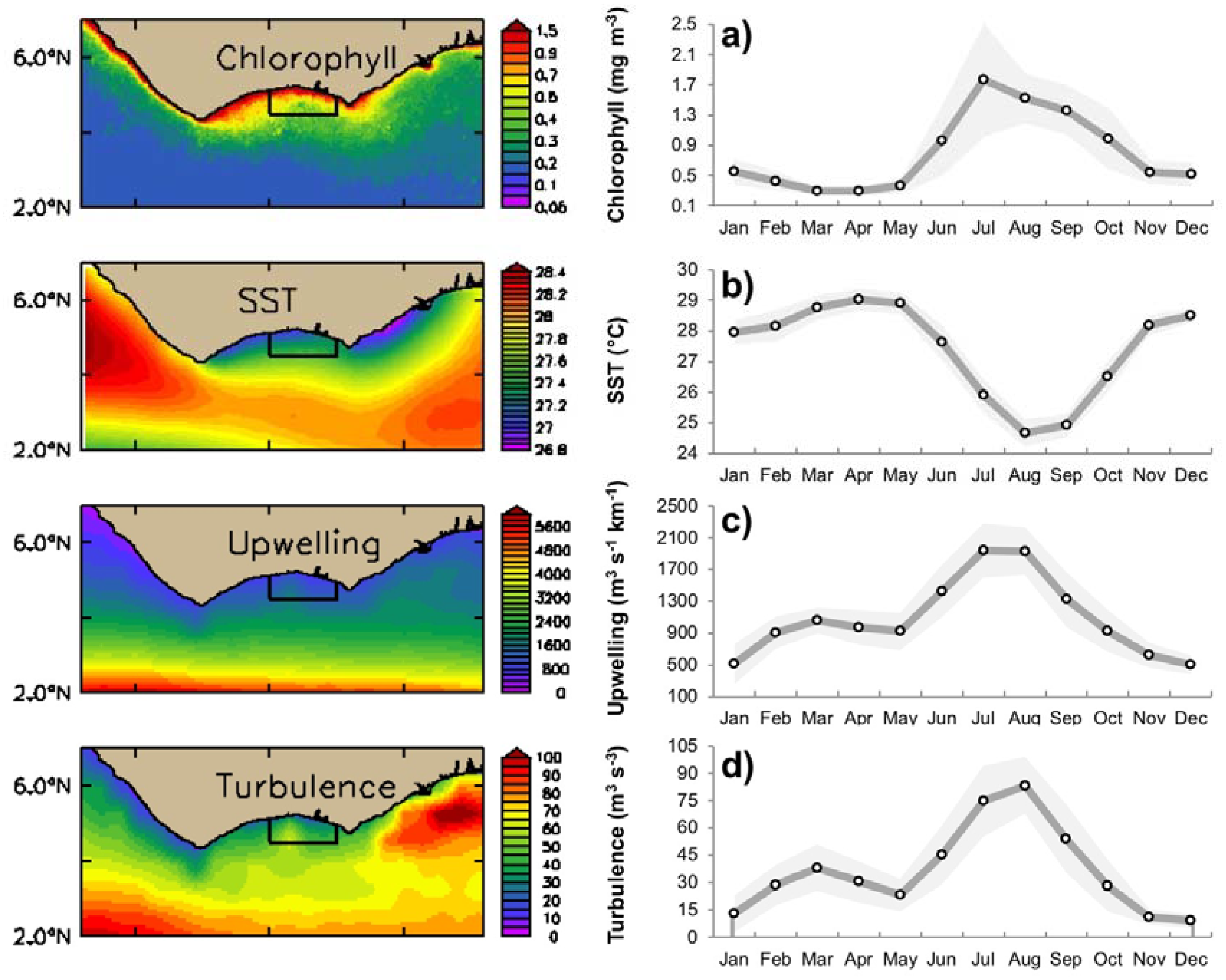
3.1. Seasonal Variability of Biophysical Drivers in Ivorian Waters

The seasonal variations of chlorophyll pigment concentration and SST in the fishing zone of Abidjan are shown in Figure 2a,b and Figure 3a. High phytoplankton blooms with chlorophyll concentrations of ~1.7 mg m⁻³ are observed in coastal waters during the period from July to September, which corresponds to the period of intense upwelling and low SST. Phytoplankton variability follows seasonal fluctuations in SST.

The SST value increases from 27.5 to 29 °C from January to April, followed by a gradual decrease from April to August, to a minimum value of 24 °C. Finally, the SST increases until December to reach the maximum value of 28.5 °C. We observe that cold water is present over the entire Ivorian coastal zone during the major cold season, with an average temperature of 24 °C. During this season, the coldest surface temperatures are observed in the central and eastern parts of the littoral between 5 and 2°W during the month of August. Warmer temperatures are found in the western part between longitudes 7°W and 8°W during the month of July.

The seasonal variation in coastal upwelling in the fishing zone of Abidjan is shown in Figure 2c. The upwelling index increases from 500 m³ s⁻¹ km⁻¹ in January to 1100 m³ s⁻¹ km⁻¹ in March, then decreases slightly in May to 750 m³ s⁻¹ km⁻¹. From June, there is a rapid and maximal increase in upwelling index, reaching values of 2000 m³ s⁻¹ km⁻¹ in July–August. Finally, values decrease gradually to reach 500 m³ s⁻¹ km⁻¹ in December. In the fishing zone of Abidjan, wind-induced turbulent mixing (Figure 2d) follows the same seasonal variations as the upwelling index. Turbulent mixing increases from 10 m³ s⁻³ in January, reaching 35 m³ s⁻³ in March–April–May. Then, turbulent mixing values increase again, reaching a maximum of 80 m³ s⁻³ in July–August, before gradually decreasing to values of 10 m³ s⁻³ in December. The variations in coastal upwelling index and turbulent mixing are consistent with in situ measurements of thermocline depth, showing shallow depths between 0 and 50 m (upper and lower bounds, respectively) from July to September during the major cold season, and between 10 and 60 m from January to March during the minor cold season. The thermocline deepens to between 15 and 65 m (upper and lower bounds, respectively), on average, between April and June, and between October and December.

The seasonal distribution of depth-integrated nutrient concentration showed a rapid increase in nitrate from January to March, reaching maximal concentration in April–May, with values of 0.55 mol m⁻² on average. Nitrate concentration decreases to a minimum of 0.32 mol m⁻² in October, which is then followed by increasing concentration from November onwards. Seasonal distribution in phosphate showed lower concentrations from March to May, and then from July to August, with mean values of 0.033 and 0.025 mol m⁻², respectively. Phosphate concentration increases, again, from December to February, reaching values of 0.041 mol m⁻², on average.

3.2. Interannual Variability of Biophysical Drivers in Ivorian Waters

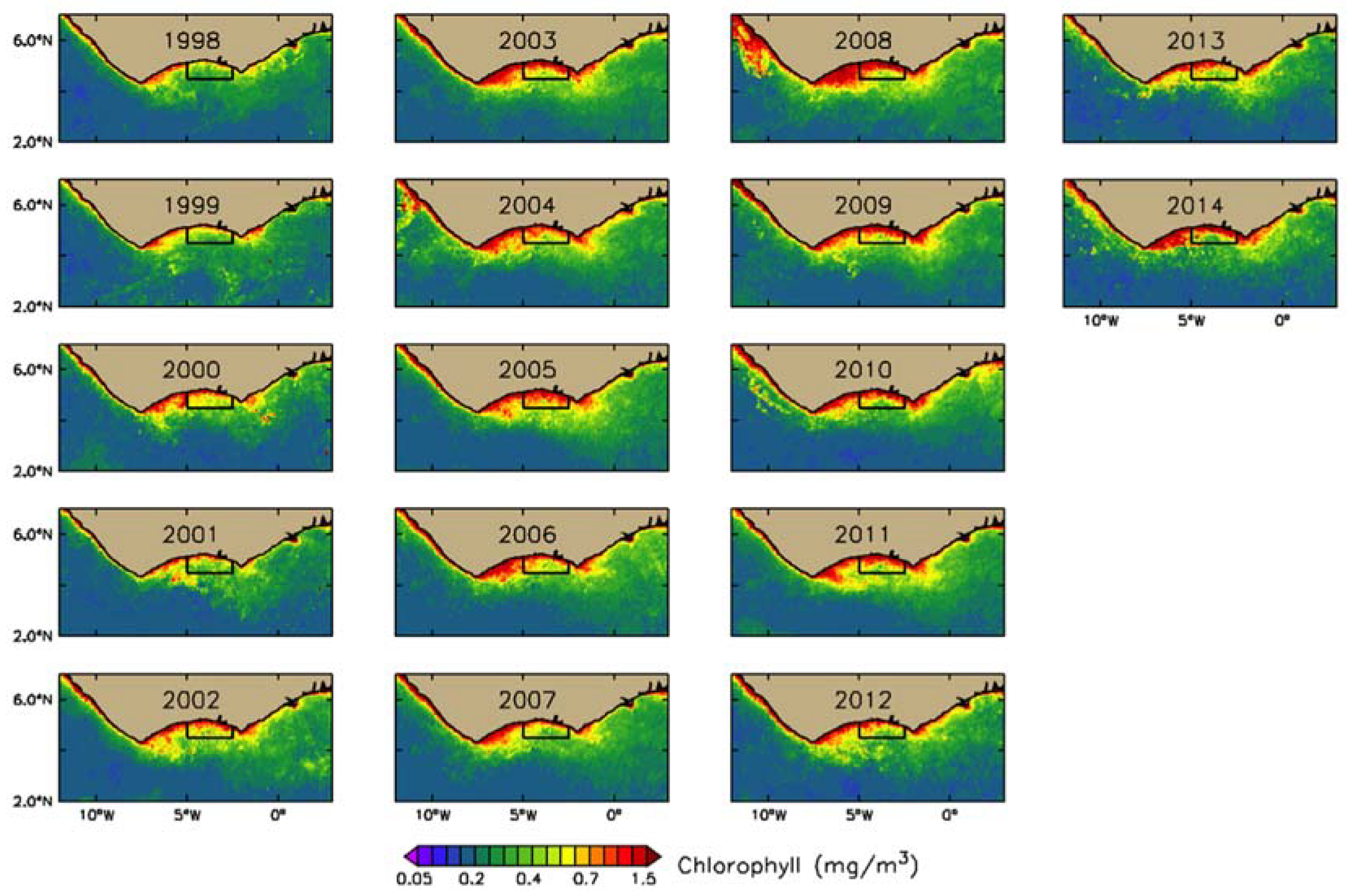
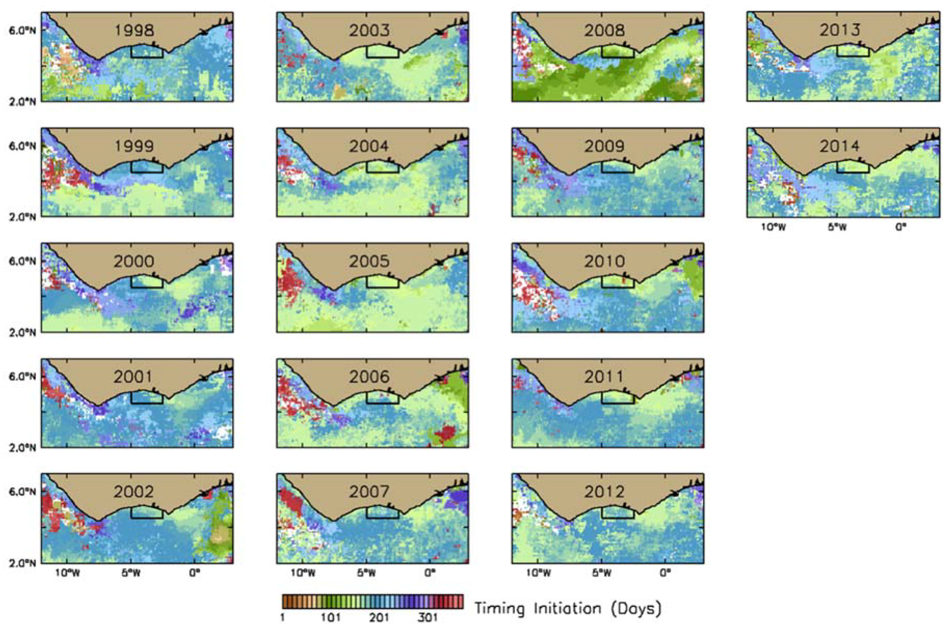
3.2.1. Phytoplankton Indices

• Spatial distribution in chlorophyll concentration anomalies

The year-to-year variations of chlorophyll concentration over the period 1998 to 2014 are represented in Appendix Figure A1 as annual means, expressed in mg Chl m⁻³, and in Figure 4 as the relative anomalies, expressed as percent change from the 1998–2014 mean. In the fishing zone of Abidjan (box area in Figure 4), negative anomalies are prominent from 1998 to 2002, then in 2007, and finally, from 2012 to 2013. The lowest relative chlorophyll anomalies (−40%) are observed in 1998, 1999 and 2001. In 2002, 2007, 2012, and 2013, the negative anomalies are in the range of −20% to −5%. In 2006, 2010, 2011, and 2014, the relative chlorophyll concentration anomalies are close to zero on average, with values lying between −5 and +5%. The positive relative chlorophyll anomalies are dominant in 2003–2005, 2008, and 2009, with a maximum percentage value of +35% in 2008.

• Spatial distribution in anomalies of phytoplankton phenology

Year-to-year variations in timing of initiation of phytoplankton growth over the period 1998 to 2014 are shown in Appendix Figure A2, and the anomalies in Figure 5. Three types of phytoplankton growth initiation times were observed from 1998 to 2014, namely early initiation (blue color in Figure 5), late initiation (indicated in red), and normal initiation (white). In the fishing zone of Abidjan, earlier than average timing of initiation between −4 and −2 weeks is observed in the years 2003–2005, 2010, 2013, and 2014, whereas in 2008, the phytoplankton growth started particularly early (−6 weeks). Moderate delay in the initiation of phytoplankton growth between +1 and +4 weeks is observed in 2007, 2009, and 2012. Longer delay, with greater than +4 weeks, are estimated for the first five years, from 1998 to 2002.

• Temporal variations in S. aurita catch, chlorophyll, and timing of initiation

In the fishing zone of Abidjan, timing of initiation of phytoplankton growth shows a synchronous relationship with S. aurita catch, i.e., when S. aurita catch is high, the timing of initiation is delayed, during the period from 1998 to 2014 (Figure 6a). Whereas analysis of S. aurita catch and concentration of chlorophyll shows an inverse relationship between the two variables (Figure 6b), i.e., when S. aurita catch is high, there is a large decrease in the concentration of chlorophyll and vice-versa. The latter relationship is observed in most of the years during the period from 1998 to 2014, except for the years 1999–2000 and from 2012 to 2014, when both variables change synchronously.

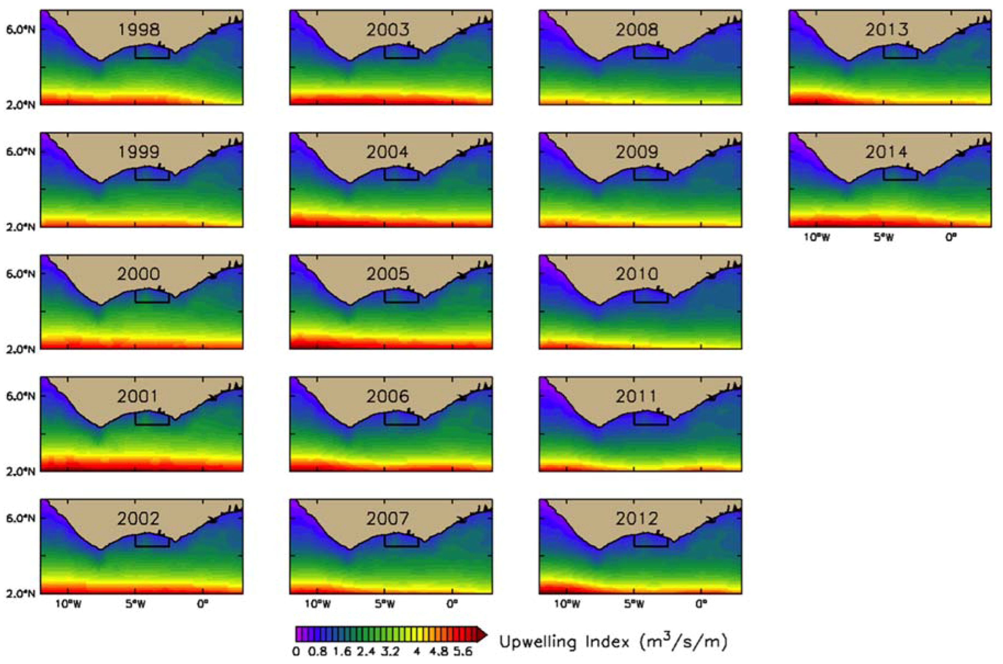
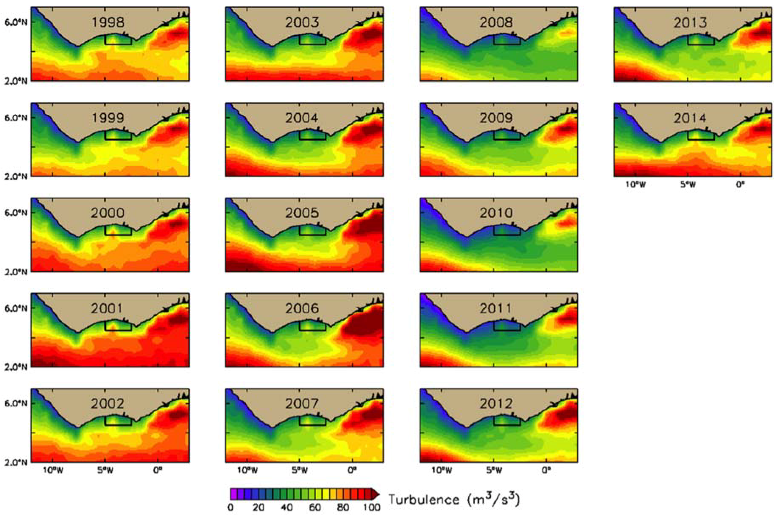
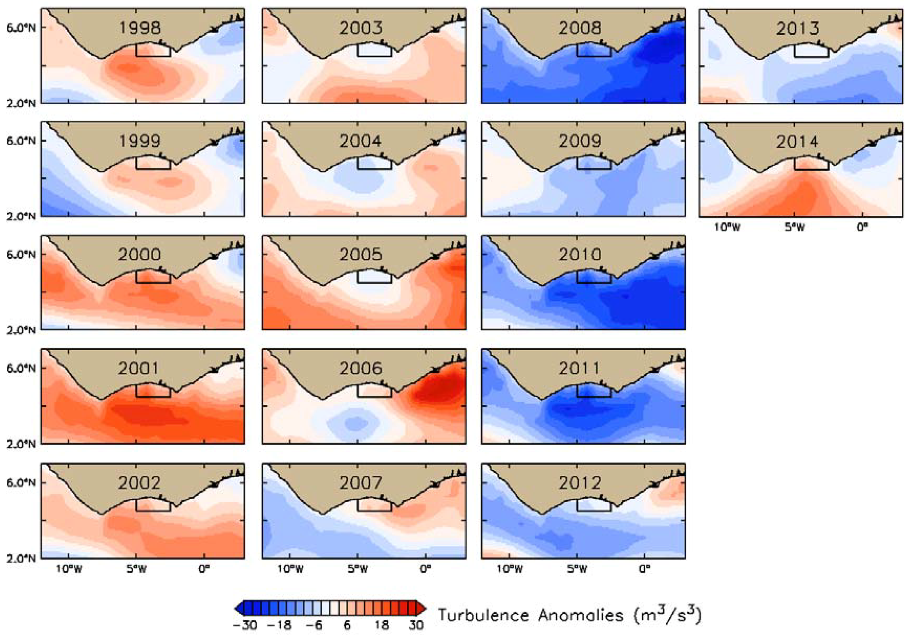
3.2.2. Physical Indices

• Spatial distribution in anomalies of upwelling index

Upwelling index is an important variable in the determination of fishing areas on the coasts. The distribution of the upwelling index for the period from 1998 to 2014 in Ivorian waters is presented in Appendix Figure A3, and the anomalies in Figure 7. In 2002, 2003, 2005, and 2007, upwelling index is close to average condition, and anomalies oscillate between −100 and 100 m³ s⁻¹ km⁻¹. In the area of the fishing zone of Abidjan, negative anomalies are observed in 1999, 2004, 2006, and from 2008 to 2012, with lowest values of −500 m³ s⁻¹ km⁻¹, while positive upwelling index anomalies are observed in the years 1998, 2000, 2001, 2013, and 2014 with maximum values of +500 m³ s⁻¹ km⁻¹.

• Spatial distribution in wind-induced turbulent mixing anomalies

The year-to-year variations in annual mean wind-induced turbulent mixing for the period 1998 to 2014 are shown in Appendix Figure A4. Wind-induced turbulent mixing anomalies are presented in Figure 8, and show similar patterns of variations to those of upwelling index anomalies (Figure 7). The years of weak or strong upwelling index anomalies correspond with the years of weak or strong turbulent mixing anomalies. In the fishing zone of Abidjan, waters appear more turbulent in 2000 and 2001, with anomalies exceeding 18 m³ s⁻³, and more stable in 2008, with values of anomalies up to −30 m³ s⁻³.

• Temporal variations in S. aurita catch, turbulent mixing, and upwelling index

In the fishing zone of Abidjan, S. aurita catch is positively related to wind-induced turbulent mixing and upwelling index (Figure 9a,b). Decreasing trends are shown in these physical variables from 2000 to 2011, associated with a decreasing trend in the quantity of S. aurita caught. Furthermore, in the first years of the time series 1999–2000, the upwelling and turbulent mixing are at their highest level, and sardine catch is high, whereas, in the years 2010 and 2011, upwelling and turbulent mixing are at their lowest, and low catches of sardines are observed.

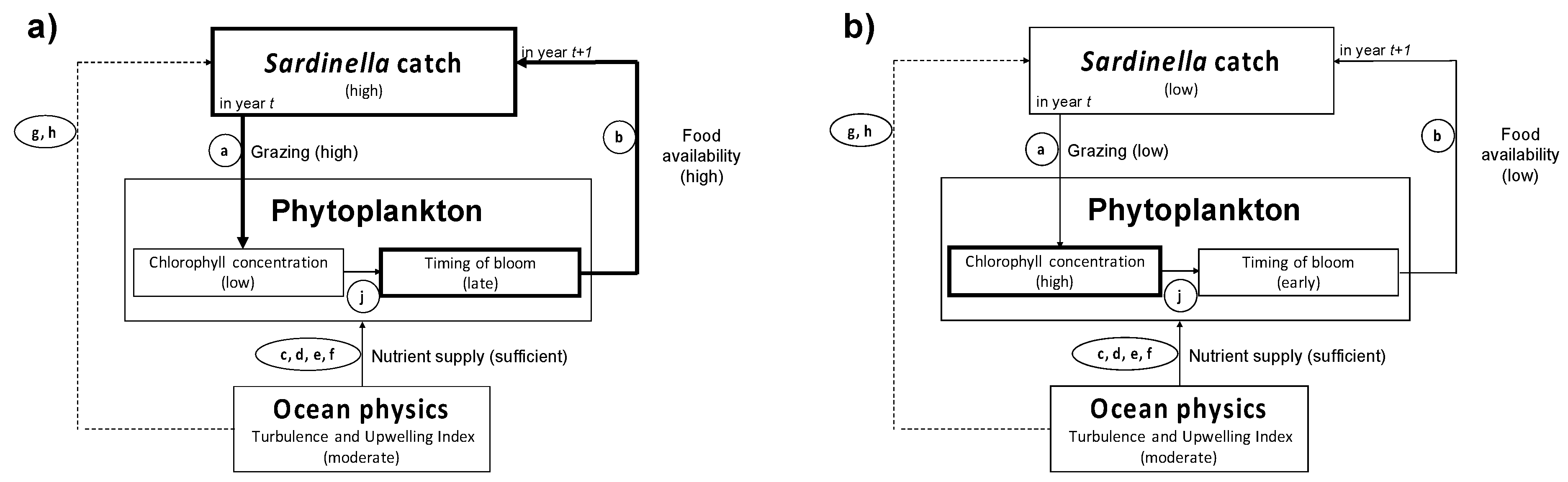
3.3. Diagnostic Model of Sardinella Catch

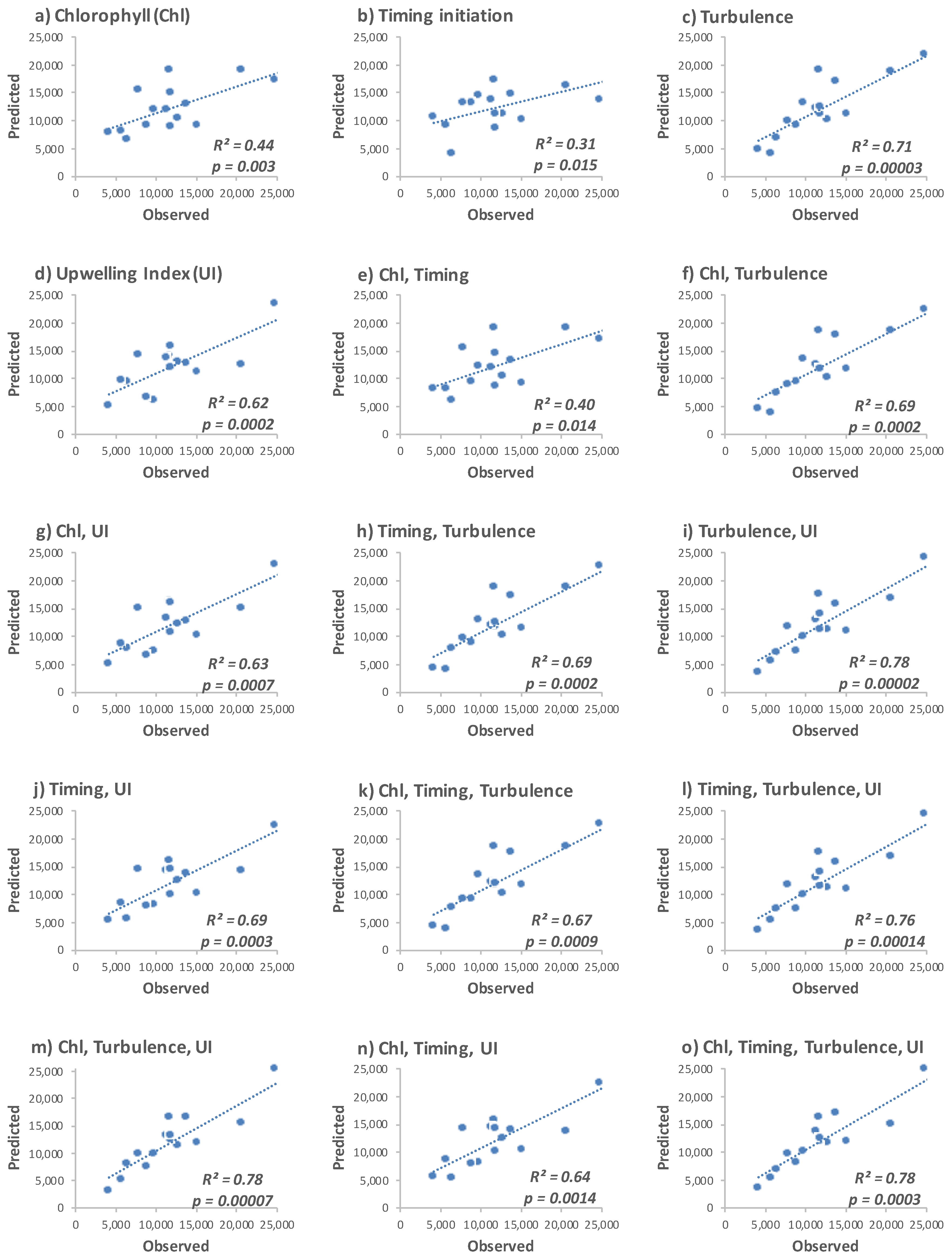
3.3.1. Empirical Relationships between Sardinella aurita and Biophysical Variables

• S. aurita catch and first trophic level

Our analysis in the fishing zone of Abidjan shows significant linear relationships between S. aurita catch and variables of chlorophyll concentration and timing of initiation (Figure 10a,b). Catches of S. aurita are inversely related to the concentrations of chlorophyll, such that low concentration of chlorophyll in year t is associated with high S. aurita catch in same year. Interannual variations in the concentration of chlorophyll can explain 48% of the variations in S. aurita catch. This negative relationship may indicate an important grazing pressure from Sardinella larvae on phytoplankton. A positive linear relationship is observed between the timing of initiation of phytoplankton growth in year t and S. aurita catch in year t + 1. Early (late) timing of initiation of phytoplankton growth is associated with low (high) S. aurita catch in the following year. If the timing of phytoplankton bloom occurs earlier (negative anomaly) than average conditions, a mismatch may be observed between food availability (phytoplankton) and the arrival of Sardinella larvae. Under such conditions, survival of Sardinella larvae may be low, which may then translate into low adult fish recruitment and consequent low catch in year t + 1. By contrast, delay in the timing of phytoplankton blooms (positive anomalies) may bring more favorable conditions for the survival of Sardinella larvae (good timing of food availability), which may then allow for high adult fish recruitment and their catch in year t + 1.

• S. aurita catch and ocean physics

Our analysis in the fishing zone of Abidjan shows significant positive linear relationships between S. aurita catch, and the dynamics of the physical variables of upwelling index and wind-induced turbulent mixing (Figure 10c,d). For moderate turbulent mixing (from June to December) and favorable upwelling (annual mean), there is generally good recruitment of S. aurita on the Ivorian continental shelf. High upwelling index may increase nutrients and food availability to the surface waters, bringing favorable feeding conditions for the Sardinella, and leading to higher catches. In addition, the turbulent mixing of the months from June to December presents favorable conditions for a strong increase in nutrients in the coastal regions. In this context, high wind-induced turbulent mixing is shown to be positively related to S. aurita catch, with turbulent mixing explaining 69% of the variations in S. aurita catch from 1998 to 2014.

• First trophic level and ocean physics

Our analysis in the fishing zone of Abidjan shows significant positive linear relationships between phytoplankton and ocean physics (Figure 10e–h). On the one hand, the high upwelling index and wind-induced turbulent mixing observed in the present analysis allow sufficient nutrient supply for phytoplankton to grow and develop in a bloom, such that bottom-up trophic interactions may not be a limiting factor. On the other hand, favorable environmental conditions may lead to enhanced grazing pressure by Sardinella larvae, exerting important top-down control on the phytoplankton (low chlorophyll concentration), such that increased turbulent mixing and upwelling index may be associated with good recruitment of S. aurita larvae, increasing grazing pressure on phytoplankton, leading to lower chlorophyll concentration, and a delayed bloom initiation, i.e., time when chlorophyll reaches the threshold of median plus 20% (Figure 10b).

3.3.2. Linear Regression Analysis and Model Equation

Based on the empirical relationships demonstrated between S. aurita catch and physical-biological variables (Section 3.3.1), diagnostic models for prediction of S. aurita catch in the fishing zone of Abidjan can now be explored. To identify the best combination of predictors, we performed an exhaustive search over all possible combinations of input variables derived from two biological and two physical variables (i.e., there are 15 possible combinations out of four variables). The bilinear regression model using only the biological variables (timing of initiation of phytoplankton growth and chlorophyll concentration) can explain 40% of the variations in S. aurita catch, whereas the model using only the physical variables (upwelling index and turbulent mixing) shows that in year t, these two variables may allow us, with a confidence of 78%, to predict S. aurita catch in year t + 1 (Figure 11e,i). The latter score is also observed in the multilinear regression model using chlorophyll concentration, upwelling index and turbulent mixing as predictors (Figure 11m), as well as in the multilinear regression model using timing of initiation of phytoplankton growth, chlorophyll concentration, upwelling index, and turbulent mixing as predictors (Figure 11o). However, statistical analysis of the coefficient estimates indicates that only the variables turbulent mixing and upwelling index significantly improve the fit of these models.

Based on these results, we provide the predictive equation using only the physical variables, as follows:

$$S. Catch\left(t+1\right)= -40 \times {10}^3+12 \times {10}^3\times Chl\left(t\right)+535\times Timing\left(t\right)+444\times Turbulence\left(t\right)+21\times UI\left(t\right)$$

(3)

However, although the physical variables may be statistically better predictors of the variations in S. aurita catch in year t + 1, they have no direct influence on the trophic interactions of this species. To assess how much the variations in S. aurita catch in year t + 1 can be explained by changes at the base of the marine food chain (i.e., phytoplankton food availability), we need to consider predictive models using biological variables as predictors (Figure 11a,b,e). We found that phytoplankton chlorophyll concentration and bloom timing initiation alone can explain 44% and 31% of S. aurita catch in year t + 1, respectively (Equations (2) and (3)), and that the combination of these two variables can explain 40% of the variations in S. aurita catch (Equation (4)). The equations describing these linear models are given as follows:

$$S. Catch\left(t+1\right)= 30 \times {10}^3-21 \times {10}^3\times Chl\left(t\right)$$

(4)

$$S. Catch\left(t+1\right)= 12\times {10}^3-2 \times {10}^3\times Timing\left(t\right)$$

(5)

$$S. Catch\left(t+1\right)= 28 \times {10}^3-19 \times {10}^3\times Chl\left(t\right)+248\times Timing\left(t\right)$$

(6)

4. Discussion

4.1. Seasonal and Interannual Variability in Biophysical Conditions

The SST along the Ivorian coastline is characterized by large seasonal variations [61,62]. Based on these thermal variations, four marine seasons have been defined: the minor cold season from January to February; the major warm season from March to June, with a maximum temperature centered on the month of May; the major cold season from July to September; and finally, the minor warm season from November to December. Our results showed that the peaks of chlorophyll concentration, upwelling index, and wind-induced turbulent mixing generally coincide with low SST. In support of our results, similar observations have been previously reported in several studies based on in situ measurements [61,62,63,64,65] and a hydrodynamic regional model [37], describing the seasonal development of the upwelling (the resurgence of cold water) off the Côte d’Ivoire. Highest intensity of upwelling is observed from July to September. During this period, upwelling enriches the ocean with nutrients, with immediate influence on primary production [25,31,66]. Nutrient enrichment has been shown to control the development of phytoplankton, such that chlorophyll and nitrate concentrations may be linearly related during the months of July and August [67], and the phenomenon of upwelling can be localized by the presence cold seawater that is rich in phytoplankton. In situ measurements of nitracline depth-integrated nitrate concentration and phosphatocline depth-integrated phosphate concentration (Figure 3c,e respectively) indicate that phytoplankton consume nutrients (decreasing concentration in July to August). However, nutrient depletion is not observed, suggesting that nutrient availability may not be limiting phytoplankton growth during the major cold season, and other factors may play an important role, including grazing and light availability. Influence of grazing is discussed in detail in Section 4.2. The role played by the light availability in controlling phytoplankton production in Ivorian waters has been previously assessed by Herbland and Voituriez [67], who demonstrated that the depth of the thermocline may be inversely related to the slope of the chlorophyll-a concentration and in vivo fluorescence. In the region, previous studies [68,69,70] have also reported that when the wind is at the origin of the upwelling, it causes mixing that can be associated with reduced light availability within the mixed layer, which can become one of the factors limiting production. Further increase in wind speed may also increase the speed of surface currents, which can drive phytoplankton-rich waters towards the open ocean. Such changes in wind conditions may change availability of food (phytoplankton) for fish larvae and affect fish recruitment (see Section 4.2).

Although upwelling is the main source of enrichment in the euphotic zone of the littoral, the contribution of the discharges of the main rivers should not be ignored [30]. According to Binet [23], and Herbland and Le Loeuff [25], during the great warm season, terrigenous contributions may be provided to the Ivorian coastal zone. These nutrient-rich inputs come from runoff from the land surrounding the coastal lagoons, and peak in October [71]. They are especially important in the eastern part of the coast, and may increase the concentration of phytoplankton in the area [29].

4.2. Influence of Biophysical Conditions on the Recruitment of Sardinella Aurita

Coastal upwelling ecosystems are known to be highly productive [18,72]. Generally, fish avoid breeding in areas dominated by strong currents and water column mixing. The spawning sites are usually located downstream from the main upwelling centers, and breeding is mainly tuned to avoid the peak of the upwelling season [73]. On the Ivorian continental shelf, we show that SST is low at the coast, and increases towards the open sea, whereas chlorophyll concentration is high at the coast and decreases towards the open sea. In this area, phytoplankton and other biological components retained at the coast provide favorable conditions for the reproduction of S. aurita. Our results are in good agreement with those of Roy [73], who reported, during a study of upwelling-induced retention area off Senegal, that the coastal zone represents a very favorable environment for fish reproduction. The author indicated that eggs and larvae might develop in productive and relatively stable coastal waters. In the Ivorian continental shelf, upwelling and coastal retention of larvae occur simultaneously and, together, provide favorable conditions for fish reproduction.

In the present study, we have shown a significant linear relationship between upwelling index and wind-induced turbulent mixing strength, suggesting the presence of an Ekman-type upwelling system, according to the definition by Cury and Roy [74]. The latter authors report the existence of an “optimal environmental window” for the recruitment of sardines, which is characterized by moderate values of turbulent mixing and upwelling index. Along the Ivorian continental shelf, during the period 1998–2014, turbulent mixing and upwelling index remained within the range of moderate values, 800 to 1400 m³ s⁻³, and 30 to 60 m³ s⁻¹ km⁻¹, respectively (Figure 10), which are commensurate with values identified by Cury and Roy [74], suggesting that throughout the period of study, the ocean physical conditions were “optimal” for fish recruitment. In addition, during the major upwelling, nutrient concentration is shown to be sufficient (Figure 3d,f; [71]), supporting the growth of phytoplankton. In these conditions, bottom-up control may not be the limiting factor for the recruitment of Sardinella larvae, and the observed year-to-year variations in S. aurita catch may be driven by top-down control (Figure 12a,b).

In the Ivorian shelf waters, S. aurita spawns during or after the cold season (June to September), and the highest abundance of larvae is observed in August [75]. The diet of Sardinella larvae may include small crustaceans (copepods), but, along the coasts of Senegal, Congo [76,77], Côte d’Ivoire [78], and Ghana [79], their main source of food has been shown to be phytoplankton. In the Congolese fishery of S. aurita, Ghéno and Fontana [80] have observed that the variability in spawning in the previous seasons is reflected in a strong variability of the catch rates of the fishery. Furthermore, enhanced S. aurita catch in the Ivorian fishery has been observed when the onset of the phytoplankton bloom occurs early in April–May, just preceding the main spawning and recruitment period of S. aurita between June and October (with a maximum in July–August; [81,82]). During this period, the vulnerability of fish stocks to fishing activities is particularly high [36,83,84,85]. These reports are consistent with our findings of a positive relationship between the phytoplankton bloom timing and the S. aurita catch in the following year, which may be further explained as follows (Figure 10): in the years when the phytoplankton flowering begins early (e.g., negative anomalies of ~2–4 weeks; Figure 10a), seasonal chlorophyll concentration (i.e., food availability) is high when Sardinella larvae are released, and the larvae have sufficient food in their critical period to eat on and grow. Such conditions are favorable for successful recruitment of Sardinella larvae, and lead to a higher Sardinella catch in the year t + 1. In the years when phytoplankton flowering is delayed (e.g., positive anomalies of ~2–4 weeks; Figure 10a), the amount of food available (i.e., chlorophyll concentration) to the larvae is low, and larvae may die by starvation. In such conditions, Sardinella larval recruitment is low, and the Sardinella catch in the following year may remain low.

During the period of study 1998–2014, year-to-year variations in Sardinella larvae are not available to allow direct validation of the match–mismatch hypothesis [86] between Sardinella larvae and phytoplankton bloom timing. However, we also observed negative relationships between phytoplankton chlorophyll concentration in year t and Sardinella catch in the same year t, suggesting that Sardinella larvae exert a significant grazing pressure on phytoplankton. Hence, to provide an indirect validation of the hypothesis about the relationship between Sardinella recruitment and phytoplankton availability, we next estimate, empirically, the carbon consumption rate by Sardinella larvae in the area based on the relationship demonstrated in Section 3.3.1; and we then compare this estimate with in situ consumption rates of Sardinella larvae reported in the literature.

• Estimation of carbon consumption rate in the study area

Figure 10a shows, for different years, the total sardine catch (a proxy for abundance) plotted against the annual average of chlorophyll concentration in the same years. In the years when the abundance of sardines is high, the chlorophyll is low (and vice versa), implying a role for grazing on chlorophyll by sardines. From the slope of the regression line (i.e., 22 × 10³ tons sardines per mg Chl m⁻³), we could infer that an increase in sardine population of 22 × 10³ tons would be associated with a decrease in chlorophyll of 1 mg m⁻³, averaged over the study area. We interpret this decrease as the average food supply required to sustain the increase in sardine abundance, and make the assumption that the 1 mg m⁻³ of chlorophyll represents the average daily food consumption of 22 × 10³ tons. Finally, we proceed to estimate the carbon consumption rate in the study area of the Abidjan fishing zone, which is characterized by a surface of 2 × 10¹² m², and mixed layer depth of 60 m (the latter value is based on vertical profiles of chlorophyll concentration measured in front of Abidjan during the sampling campaign reported in Herbland and Voituriez [67]. By multiplying the consumption rate of 1 mg Chl m⁻³ day⁻¹ by the depth of the mixed layer and surface of the study area, we calculate the total amount of chlorophyll consumed to be 4.4 × 10¹⁶ mg Chl year⁻¹. Assuming a carbon (C) to Chl ratio of 50 [87], we obtain a monthly consumption rate of carbon of 1.9 × 10¹⁷ mg C month⁻¹ or 2.5 × 10¹⁷ μg C h⁻¹.

• Estimation of larval abundance and consumption rate

Assuming that adult Sardinella weighs, on average, 229 g [88], the number of Sardinella in the water volume of the study area would be 5 × 10¹² individuals or 0.04 individuals per m³. We hypothesize that half of the individual Sardinella are females, and each female produces an average of 80,000 larvae [89]. Then, we obtain the total number of larvae, 2.1 × 10¹⁷, in the water volume of the study area, or about 1700 larvae per m³. Finally, the carbon consumption rate may be divided by the total number of larvae, which gives 1.2 μg C larva⁻¹ h⁻¹. The latter result is within the same order of magnitude compared to previously published figures by Caldeira et al. [90], who reported carbon intake rates for sardine species Sardina pilchardus in European waters between 4.5 and 7 μg C larva⁻¹ h⁻¹. The relatively lower carbon consumption rate observed here for Sardinella aurita may be due to the fact that (1) the European Sardina pilchardus is likely to present anatomical and physiological differences, as well as living in different environmental conditions, compared with the species Sardinella aurita studied here in Ivorian waters; and (2) our calculation is based on total Sardinella catch, and this value is likely to underestimate the total number of Sardinella individuals present in the study area (i.e., not all Sardinella may have been caught).

4.3. Relevance of Remote-Sensing Observations and Diagnostic Models for Sardinella Fisheries Management and Operational Applications

Since the intensification of fishing activity and the increase in awareness of the need to monitor fish stocks closely, evaluation methods and reporting of fish catches have been progressively standardized at national and international levels. To date, 441 of the 584 commercial stocks of marine animals throughout the world are routinely evaluated [91].

With a continental shelf of 12,000 km², the Côte d’Ivoire is among the poorest countries in fishery resources in the area of the Gulf of Guinea. Small pelagics, whose abundance depends on environmental conditions, such as the seasonal appearance of coastal cold water, are estimated to be 81,000 tons between Togo, Ghana, and Côte d’Ivoire [92]. In recent years, several analyses have reported the collapse and scarcity of a large number of commercially important fish stocks across these countries [93,94,95]. The continuous increase in fishing pressure beyond self-renewal capability of already limited fish stocks, is identified as the main cause of declining abundance of the fishery resource, and represents the greatest threat to the sustainable development of fishing activity in the region [96,97].

Sardinella aurita plays a significant role in the profitability of the fishing industry, and is mainly responsible for supplying local consumers and neighboring regions with protein-rich, high-quality food at a low price. However, the structures responsible for the management of the Ivorian fishery face several difficulties. There is a lack of information in the sector as a whole, with weak decision-making tools, weak policy and regulatory frameworks, and poverty in fishing communities. To tackle these issues, we propose that the biophysical metrics of phytoplankton phenology, phytoplankton biomass, turbulence, and upwelling index, identified in the present study, be incorporated into stock assessments within an ecosystem-based management framework for Côte d’Ivoire. The metrics may be readily, objectively, and freely estimated from remote-sensing and reanalysis products, and they meet operational requirements in terms of spatiotemporal resolution, repeat frequency, and cost-effectiveness [12]. Furthermore, we have demonstrated that, applied in a multilinear diagnostic model, these biophysical metrics may allow us, with a confidence of 78%, to predict the S. aurita catch in the following year.

In this context, we suggest the following approach towards an implementation of a Fisheries Information and Management System for Ivorian waters:

(1)

On a monthly basis, retrieval of data metrics, mapping of metric anomalies, and plotting of time-series metrics;

(2)

On a yearly basis, estimation of annual mean S. aurita catch, annual mean upwelling index, June to December mean wind-induced turbulent mixing, annual mean chlorophyll concentration, calculation of long-term chlorophyll threshold criterion and timing of initiation of the phytoplankton growing period;

(3)

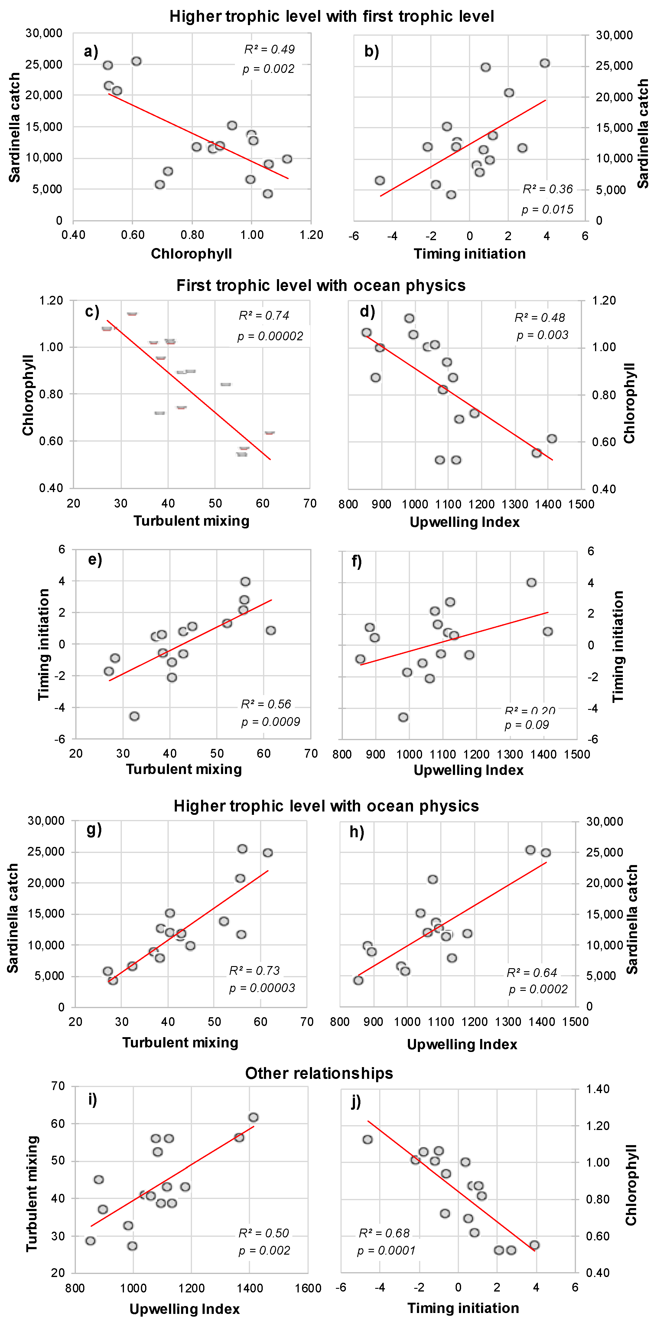
Analysis of empirical relationships between S. aurita catch and the four biophysical variables, using data for all available years from 1998 to present;

(4)

If the empirical relationships are significant, estimate the new parameters of the multilinear diagnostic model and forecast, with confidence levels, the S. aurita catch in the following year; If the empirical relationships are not significant, further analyses and search of optimal diagnostic model need to be performed in consultation with experts from CURAT or other institutes, as relevant;

(5)

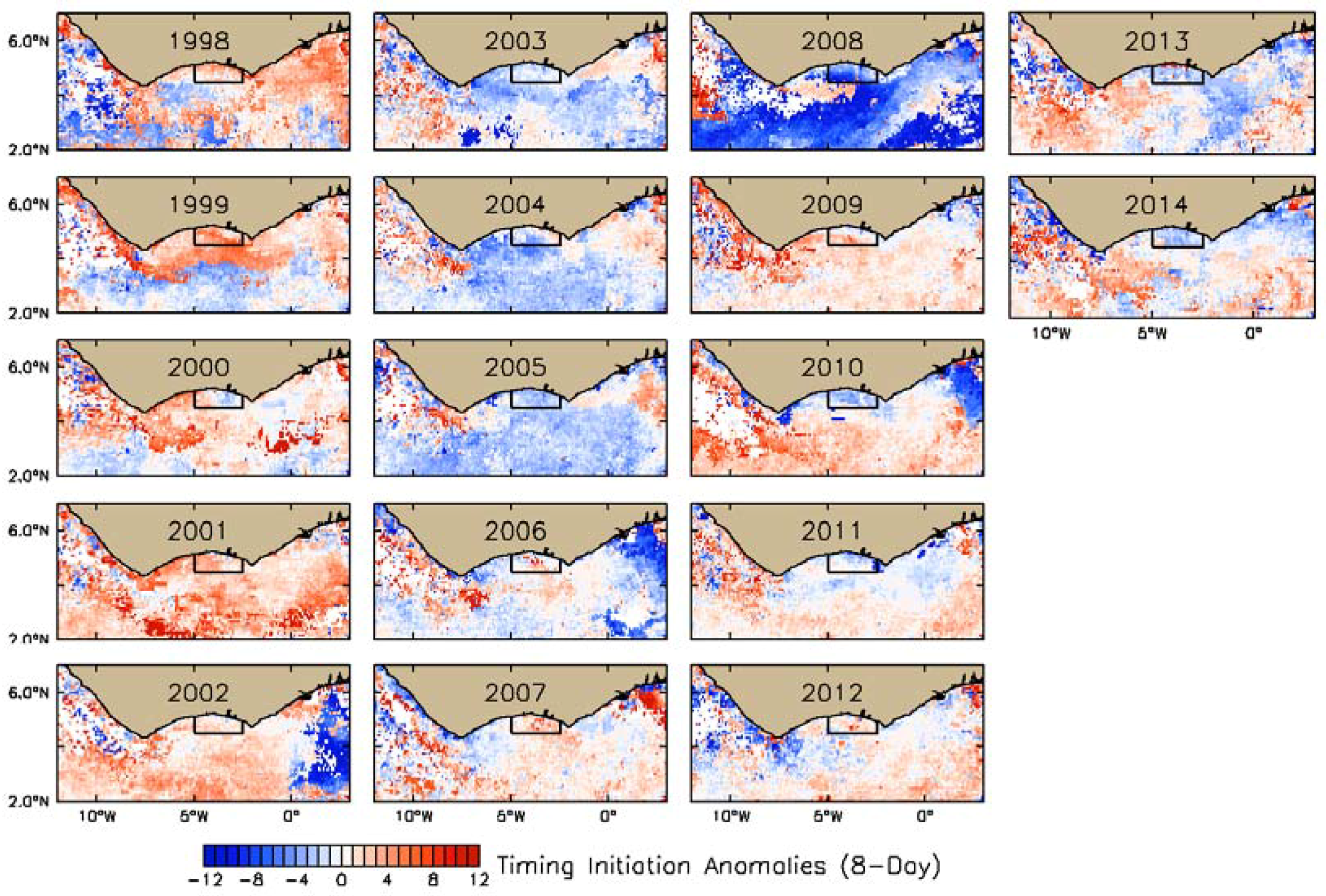
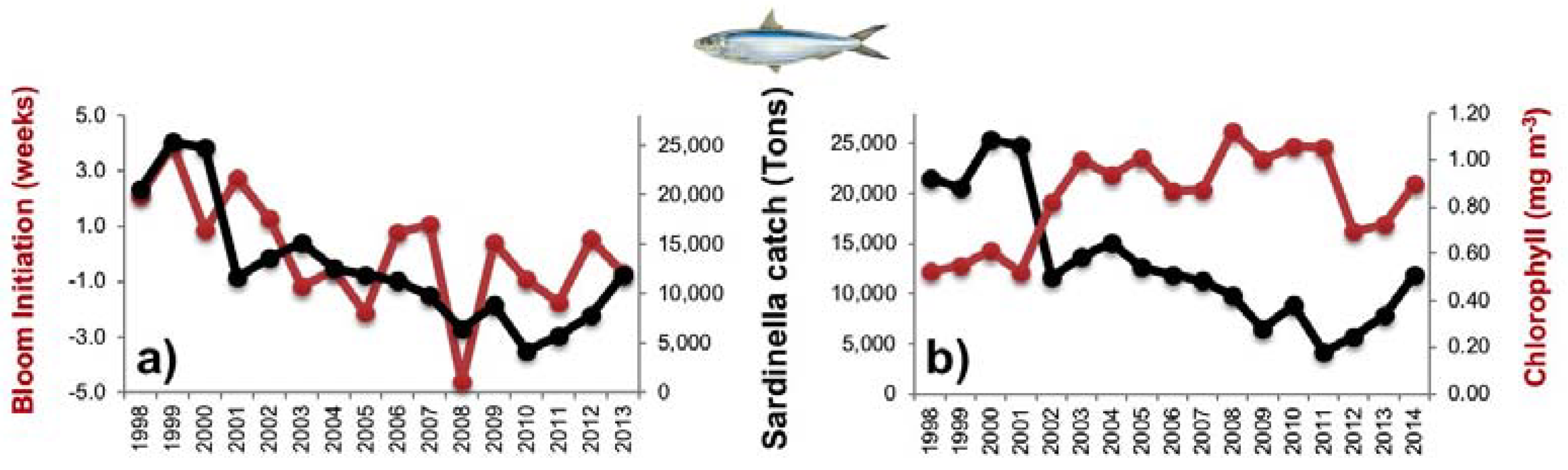
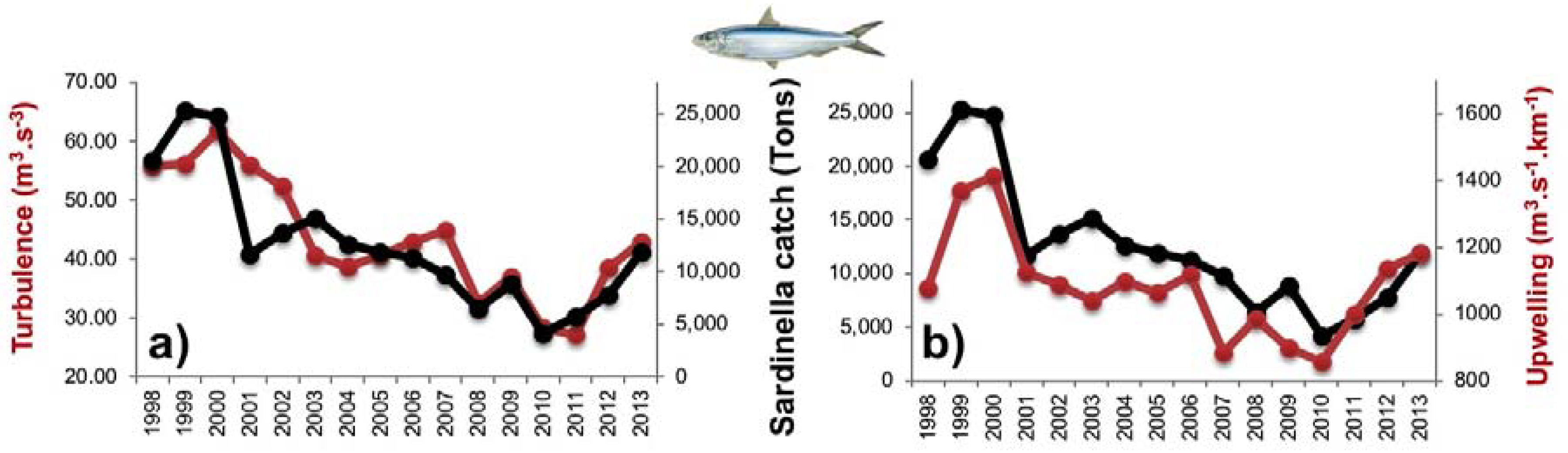
Produce an information bulletin providing an annual summary of biophysical metric status, including anomaly maps (such as presented for instance in Figure 4, Figure 5, Figure 7, and Figure 8), time-series plots (for instance, as in Figure 6 and Figure 9), and the estimate, with a confidence level, of S. aurita catch forecast for the following year;

(6)

Review the information bulletin with the representatives in charge of the S. aurita stock assessment and issue advice on protection measures, as required;

(7)

Provide evidenced-based management advice to government agencies, enabling them to make informed decisions.

5. Conclusions

In this study, a regression model based on physical variables has been shown to explain 78% of the catch of Sardinella aurita in the following year (year t + 1) when the annual mean upwelling index and mean wind-induced turbulent mixing in the months of Jun to Dec of the current year (year t) are known. On the other hand, the regression model based on biological variables of the timing of phytoplankton bloom initiation and chlorophyll concentration has been shown to explain 40% of the catch of Sardinella aurita in the following year. Although the physical variables may, statistically, be better predictors of the variations in Sardinella catch in the following year, we have highlighted that, during the period 1998–2014, the upwelling and turbulence strengths have remained of moderate intensity, suggesting non-limiting nutrient supply to primary producers and trophic interactions, primarily driven by top-down control. In this context, analysis and incorporation of biological variables (into predictive models) is essential to identify alterations in trophic interactions, and to understand the fluctuations in commercially-important fisheries, such as Sardinella. Moreover, even though the predictive models developed here are based on nearly two decades of data, their parameters may be influenced by interdecadal variability and long-term regime shifts [98,99,100,101]. Examining the relationships between interdecadal climate oscillations and biological variables, such as phytoplankton phenology, as well as between other physical variables, such as precipitation and river discharge, and biological variables, may provide further insights toward improving projection of Sardinella catch in the Ivorian waters. This would bring further strength and robustness to the predictive tools, and to the proposed approach towards implementation of a Fisheries Information and Management System for Ivorian waters, which would help to lay the foundation for long-term economic growth and sustainability for the benefit of this species, and for society itself.

References

1. Fréon, P. Les Grands Écosystèmes Mondiaux D’upwelling. Les Dossiers Thématiques de L’IRD. 2006. Available online: http://www.suds-en-ligne.ird.fr/ecosys/upwelling/upwelling.htm (accessed on 21 November 2017).
2. Sherman, K. Sustainability of resources in large marine ecosystems. In Food Chains, Yields, Models, and Management of Large Marine Ecosystems; Sherman, K., Alexander, L.M., Gold, B.D., Eds.; Westview Press: Boulder, CO, USA, 1991; Volume 1, 320p. [Google Scholar]
3. Bakun, A. Guinea Current Upwelling. Nature 1978, 271, 147–150. [Google Scholar] [CrossRef]
4. Arfi, R.; Pezennec, O.; Cissoko, S.; Mensah, M. Variation spatiale et temporelle de la résurgence ivoiro-ghanéene. In Pêcheries Ouest-Africaines. Variabilité, Instabilité et Changement; Cury, P., Roy, C., Eds.; Orstom: Paris, France, 1991; pp. 162–172. [Google Scholar]
5. Arfi, R.; Pezennec, O.; Cissoko, S.; Mensah, M. Évolution temporelle d’un indice caractérisant l’intensité de la résurgence ivoiro-ghanéenne. In Environnement et Ressources Aquatiques de la Côte d’Ivoire; Le Loeuff, P., Koutia, A., Eds.; Orstom: Abidjan, Côte d’Ivoire, 1993; pp. 111–122. [Google Scholar]
6. Kassi, A.J.-B. Caractérisation et Suivi des Zones D’Upwelling Pour la Détermination des Zones de Rétention des Espèces Pélagiques Dans le Golfe de Guinée à L’Aide de la Télédétection et du Système D’Information Géographique: Cas de la Côte d’Ivoire. Ph.D. Thesis, Université Felix Houphouet-Boigny, Abidjan, Côte d’Ivoire, 2012; 124p. [Google Scholar]
7. Binet, D. Influences des variations climatiques sur la pêcherie des Sardinella aurita ivoiro-ghanéenne: Relation sécheresse-surpêche. Oceanol. Acta 1982, 5, 443–452. [Google Scholar]
8. Chika, N.U.; Chidi, A.I.; Kenneth, S. A sixteen-country mobilization for sustainable fisheries in the Guinea Current Large Marine Ecosystem. Ocean Coast. Manag. 2006, 49, 385–412. [Google Scholar]
9. Bakun, A.; Parrish, H.P. Turbulence, transport, and pelagic fish in the California and Peru current systems. CalCOFI Rep. 1982, XXIII, 99–112. [Google Scholar]
10. Bakun, A.; Roy, C.; Cury, P. The comparative approach: Latitude dependence and effects of wind forcing on reproductive success. Sess. V SARP 1991, 45, 1–12. [Google Scholar]
11. Platt, T.; Fuentes-Yaco, C.; Frank, K. Spring algal bloom and larval fish survival. Nature 2003, 423, 398–399. [Google Scholar] [CrossRef] [PubMed]
12. Platt, T.; Sathyendranath, S. Ecological indicators for the pelagic zone of the ocean from remote sensing. Remote Sens. Environ. 2008, 112, 3426–3436. [Google Scholar] [CrossRef]
13. Heath, M.R. Field investigations on the early life stages of marine fish. Adv. Mar. Biol. 1992, 28, 1–174. [Google Scholar]
14. Hjort, J. Fluctuations in the great fisheries of northern Europe, viewed in the light of biological research. In Rapports ET Proces-Verbaux. International Council for the Exploration of the Sea; Andr. Fred. Host & Fils: Copenhagen, Denmark, 1914; Volume 20, 228p. [Google Scholar]
15. Lasker, R. Field criteria for survival of anchovy larvae: The relation between inshore chlorophyll maximum layers and successful first feeding. Fish. Bull. US 1975, 73, 453–678. [Google Scholar]
16. Lasker, R.; Zweifel, J.R. Growth and survival of first-feeding northern anchovy (Engraulis mordax) in patches containing different proportions of large and small prey. In Spatial Pattern in Plankton Communities; Steele, J.H., Ed.; Plenum: New York, NY, USA, 1978; pp. 329–354. [Google Scholar]
17. Lasker, R. The role of a stable ocean in larval fish survival and subsequent recruitment. In Marine Fish Larvae, Morphology, Ecology and Relation to Fisheries; University Washington Press: Seattle, WA, USA, 1981; pp. 80–87. [Google Scholar]
18. Cushing, D.H. Plankton production and year-class strength in fish populations: An update of the match/mis-match hypothesis. Adv. Mar. Biol. 1990, 26, 249–293. [Google Scholar]
19. Koeller, P.; Fuentes-Yaco, C.; Platt, T.; Sathyendranath, S.; Richards, A.; Ouellet, P.; Orr, D.; Skúladóttir, U.; Wieland, K.; Savard, L.; et al. Basin-scale coherence in phenology of shrimps and phytoplankton in the North Atlantic. Science 2009, 324, 791–793. [Google Scholar] [CrossRef] [PubMed]
20. Iles, T.D.; Sinclair, M. Atlantic herring: Stock discreteness and abundance. Science 1982, 215, 627–633. [Google Scholar] [CrossRef] [PubMed]
21. Sinclair, M. Marine Populations: An Essay on Population Regulation and Speciation; Washington Sea Grant Program, University of Washington Press: Seattle, WA, USA, 1988; 252p. [Google Scholar]
22. Bakun, A. Comparative studies and the recruitment problem: Searching for generalizations. CalCOFI Rep. 1985, 26, 30–40. [Google Scholar]
23. Binet, D. Phytoplancton et production primaire des régimes côtiers à upwelling saisonniers dans le golfe de Guinée. Océanogr. Trop. 1983, 18, 231–335. [Google Scholar]
24. Binet, D. Zooplancton des régions côtières à upwellings saisonnières du Golfe de Guinée. Océanogr. Trop. 1983, 18, 357–380. [Google Scholar]
25. Herbland, A.; Leloeuff, P. Les sels nutritifs au large de la Côte d’Ivoire. In Environnement et Ressources Aquatiques en Côte d’Ivoire; Orstom: Paris, France, 1993; pp. 123–148. [Google Scholar]
26. John, A.W.G.; Reid, P.C.; Batten, S.D.; Anang, E.R. Monitoring Levels of “phytoplankton color” in the Gulf of Guinea Using Ships of Opportunity. In The Gulf of Guinea Large Marine Ecosystem; McGlade, J.M., Cury, P., Koranteng, K.A., Hardmann-Mountford, N.J., Eds.; Elsevier Science: Amsterdam, The Netherlands, 2002; pp. 141–146. [Google Scholar]
27. Djagoua, E.M.V. Contribution de L’Imagerie Satellitaire Visible et Infrarouge Thermique à L’Étude de la Variabilité Spatio-Temporelle des Phénomènes Physiques de Surface du Littoral Marin Ivoirien et Implication dans la Variabilité du Phytoplancton et des Prises de Sardinella Aurita. Ph.D. Thesis, Université de Cocody, Abidjan, Côte d’Ivoire, 2003; 136p. [Google Scholar]
28. Nieto, K.; Mélin, F. Variability of chlorophyll-a concentration in the Gulf of Guinea and its relation to physical oceanographic variables. Prog. Oceanogr. 2017, 151, 97–115. [Google Scholar] [CrossRef] [PubMed]
29. Dandonneau, Y. Étude du phytoplancton sur le plateau continental de Côte-d’Ivoire: III Facteurs dynamiques et variations spatio-temporelles. Cah. Orstom Sér. Océanogr. 1973, 11, 431–454. [Google Scholar]
30. Severin-Reyssac, J. Phytoplancton et production primaire dans les eaux marines Ivoiriennes. In Environnement et Ressources Aquatiques de la Côte d’Ivoire: I-Le Milieu Marin; Orstom: Paris, France, 1993; pp. 151–166. [Google Scholar]
31. Arfi, R.; Bouvy, M.; Ménard, F. Environmental variability at a coastal station near Abidjan: Oceanic and continental influences. In The Gulf of Guinea Large Marine Ecosystem: Environmental Forcing and Sustainable Development of Marine Resources; Large Marine Ecosystems Series; McGlade, J.M., Cury, P., Koranteng, K.A., Hardman-Mountford, N.J., Eds.; Elsevier: Amsterdam, The Netherlands, 2002; pp. 103–118. ISBN 0-444-51028-1. [Google Scholar]
32. Djagoua, V.; Affian, K.; Larouche, P.; Saley, B. Variabilité saisonnière et interannuelle de la concentration de la chlorophylle dans le Golfe de Guinée à partir des images SeaWiFS. Télédétection 2006, 6, 143–151. [Google Scholar]
33. Kassi, A.J.-B. Variabilité de L’Intensité de L’Upwelling Ivoiro-Ghanéen et son Impact sur la Biomasse Phytoplanctonique à L’Aide du Capteur MODIS du Satellite Aqua (2002–2005). Master’s Thesis, Université de Cocody, Abidjan, Côte d’Ivoire, 2007. [Google Scholar]
34. Kassi, J.-B.; Djagoua, E.V.; Mobio, A.B.; Gougnon, A.R.; Affian, K.; Tiemélé, J.A.; Kouadio, M.J.; Dro, C.Z.; Kouamé, A.D. Determination of the retention areas of pelagic species in Ivorian coastal water using remote sensing and geographic information system (GIS). Int. J. Sci. Eng. Res. 2014, 5, 869–877. [Google Scholar]
35. Pezennec, O.; Marchal, E.; Bard, F.X. Les espèces pélagiques côtières en Côte d’Ivoire: Ressources et exploitation. In Environnement et Ressources Aquatiques de la Côte d’Ivoire: I-Le Milieu Marin; Orstom: Paris, France, 1993; pp. 387–426. [Google Scholar]
36. Roy, C.; Cury, P.; Kifani, S. Pelagic fish recruitment success and reproductive strategy in upwelling areas: Environmental compromises. S. Afr. J. Mar. Sci. 1992, 12, 135–146. [Google Scholar] [CrossRef]
37. Koné, V.; Lett, C.; Penven, P.; Bourlès, B.; Djakouré, S. A biophysical model of S. aurita early life history in the northern Gulf of Guinea. Prog. Oceanogr. 2017, 151, 83–96. [Google Scholar] [CrossRef]
38. Fréon, P. Réponses et Adaptations des Stocks de Clupéidés D’Afrique de L’Ouest à la Variabilité du Milieu et de L’Exploitation. Analyse et Réflexion à Partir de L’Exemple du Sénégal; Etudes et Thèses; Orstom: Paris, France, 1988; 287p. [Google Scholar]
39. Massuti, O.M. La ponte de la sardine (Sardina pilchardus WALB.) dans le détroit de Gibraltar, la Mer d’Alboran, les eaux du Levant Espagnol et des Îles Baléares. Débats et Documents Techniques du Conseil Général des pêches pour la Méditerranée 1955, 3, 103–130. [Google Scholar]
40. Komarovsky, B. A study of the food of Sardinella aurita off the Mediterranean coast of Israel during a peak season (May–June 1958). Débats et Documents Techniques du Conseil Général des pêches pour la Méditerranée 1959, 5, 311–319. [Google Scholar]
41. Binet, D.; Marchal, E. The Large Marine Ecosystem of Shelf Areas in the Gulf of Guinea: Long-Term Variability Induced by Climatic Changes. In Large Marine Ecosystems: Stocks, Mitigation and Sustainability; Shermon, K., Alexander, L.M., Gold, B.D., Eds.; Wiley-Blackwell: Hoboken, NJ, USA; 1993; pp. 104–118. [Google Scholar]
42. Marchal, E. Biologie et Ecologie des poissons péIagiques côtiers. In Environnement et Ressource Aquatiques de Côte d’Ivoire: I-Le Milieu Marin; Le Loeuff, P., Marchal, E., Amon Kothias, J.-B., Eds.; Orstom: Paris, France, 1993. [Google Scholar]
43. DPH. Annuaire des Statistiques des Pêches et de L’Aquaculture Service des Études, des Statistiques et de la Documentation: Rapport D’Activité de Janvier 1997 à Décembre 2015; Direction de L’Aquaculture et des Pêches (DAP): Abidjan, Côte d’Ivoire, 2016. [Google Scholar]
44. Binet, D. Le zooplancton du plateau continental ivoirien: Essai de synthèse écologique. vOceanol. Acta 1979, 2, 397–410. [Google Scholar]
45. Sathyendranath, S.; Krasemann, H. Climate Assessment Report: Ocean Color Climate Change Initiative (OC-CCI)—Phase One. 2014. Available online: http://www.esa-oceancolour-cci.org/?q=documents (accessed on 21 November 2017).
46. Jackson, T.; Sathyendranath, S.; Platt, T. An Exact Solution for Modeling Photoacclimation of the Carbon-to-Chlorophyll Ratio in Phytoplankton. Front. Mar. Sci. 2017, 4, 283. [Google Scholar] [CrossRef]
47. Fu, G.; Baith, K.S.; McClain, C.R. The SeaWiFS Data Analysis System. In Proceedings of the 4th Pacific Ocean Remote Sensing Conference, Qingdao, China, 28–31 July 1998; pp. 73–79. [Google Scholar]
48. Steinmetz, F.; Deschamps, P.; Ramon, D. Atmospheric correction in presence of sun glint: Application to MERIS. Opt. Express 2011, 19, 571–587. [Google Scholar] [CrossRef] [PubMed]
49. Racault, M.-F.; Platt, T.; Sathyendranath, S.; Ağirbaș, E.; Vicente-Martinez, V.; Brewin, R. Plankton indicators and ocean observing systems: Support to the marine ecosystem state assessment. J. Plankton Res. 2014, 36, 621–629. [Google Scholar] [CrossRef]
50. Caddy, J.F.; Rodhouse, P.G. Cephalopod and groundfish landings: Evidence for ecological change in global fisheries. Rev. Fish Biol. Fish. 1998, 8, 431–444. [Google Scholar] [CrossRef]
51. Tzanatos, E.; Raitsos, D.E.; Triantafyllou, G.; Somarakis, S.; Tsonis, A.A. Indications of a climate effect on Mediterranean fisheries. Clim. Chang. 2014, 122, 41–54. [Google Scholar] [CrossRef]
52. Vasilakopoulos, P.; Raitsos, D.E.; Tzanatos, E.; Maravelias, C.D. Resilience dynamics and regime shifts in a marine biodiversity hotspot. Sci. Rep. 2017, 7, 13647. [Google Scholar] [CrossRef] [PubMed]
53. Fréon, P.; Mullon, C.; Voisin, B. Investigating remote synchronous patterns in fisheries. Fish. Oceanogr. 2003, 12, 443–457. [Google Scholar] [CrossRef]
54. Watson, R.; Pauly, D. Systematic distortions in world fisheries catch trends. Nature 2001, 414, 534. [Google Scholar] [CrossRef] [PubMed]
55. Froese, R.; Kleiner, K.; Zeller, D.; Pauly, D. What catch data can tell us about the status of global fisheries. Mar. Biol. 2012, 159, 1283–1292. [Google Scholar] [CrossRef] [Green Version]
56. Boyer, T.P.; Antonov, J.I.; Baranova, O.K.; Coleman, C.; Garcia, A.; Grodsky, D.R. NOAA Atlas NESDIS 72. World Ocean Database 2013; NOAA: Silver Spring, MD, USA, 2013.
57. Racault, M.-F.; Le Quéré, C.; Buitenhuis, E.; Sathyendranath, S.; Platt, T. Phytoplankton phenology in the global ocean. Ecol. Indic. 2012, 14, 152–163. [Google Scholar] [CrossRef]
58. Siegel, D.A.; Doney, S.C.; Yoder, J.A. The North Atlantic spring phytoplankton bloom and Sverdrup’s critical depth hypothesis. Science 2002, 296, 730–733. [Google Scholar] [CrossRef] [PubMed]
59. Bakun, A. Coastal Upwelling Indices, West Coast of North America, 1946–1971; NOAA Technical Report; US Department of Commerce, NMFS SSAF: Silver Spring, MD, USA, 1973; 103p.
60. Ekman, V. On the influence of the earth’s rotation on ocean-currents. Ark. Mat. Astron. Fys. 1905, 2, 1–53. [Google Scholar]
61. Moliere, A. Les saisons marines devant Abidjan. Doc. Sci. Centre Rech. Océanogr. Abidjan 1970, 1, 1–15. [Google Scholar]
62. Moliere, A.; Rebert, J.P. Etude hydrologique du plateau continental Ivoirien. Doc. Sci. Centre Rech. Océanogr. Abidjan 1972, 3, 1–30. [Google Scholar]
63. Varlet, F. Le régime de l’Atlantique près d’Abidjan (Côte d’Ivoire). Etudes Eburn. 1958, 7, 97–222. [Google Scholar]
64. Colin, C.; Bakayoko, S. Variations saisonnières des structures hydrologiques et dynamiques observées sur le plateau continental ivoirien. In Archives Scientifiques; Centre de Recherche Océanographique: Abidjan, Côte d’Ivoire, 1984; Volume 10, 64p. [Google Scholar]
65. Colin, C.; Cissoko, S. Observations hydrologiques et dynamiques le long de deux radiales du plateau continental Ivoirien pendant l’année focal 1983. In Archives Scientifiques; Centre de Recherche Océanographique: Abidjan, Côte d’Ivoire, 1984; Volume 10, 99p. [Google Scholar]
66. Koranteng, K.A.; McGlade, J.M. Climatic trends in continental shelf waters off Ghana and in the Gulf of Guinea: 1963–1992. Oceanol. Acta 2002, 24, 187–198. [Google Scholar] [CrossRef]
67. Herbland, A.; Voituriez, B. Relation chlorophylle-a—Fluorescence in vivo dans l’atlantique tropical influence de la structure hydrologique. Cahiers O.R.S.T.O.M. Série Océanographie 1977, XV, 67–77. [Google Scholar]
68. Micheli, F. Eutrophication, fisheries and consumer-resources dynamics in marine pelagic ecosystems. Science 1999, 285, 1396–1398. [Google Scholar] [CrossRef] [PubMed]
69. Jacques, G.; Treguer, P. Ecosystèmes pélagiques marins. In Collection d’Ecologie; Masson: Paris, France, 1986; 243p. [Google Scholar]
70. Ryan, J.P.; Davis, C.O.; Tufillaro, N.B.; Kudela, R.M.; Gao, B. Application of the Hyperspectral Imager for the Coastal Ocean to Phytoplankton Ecology Studies in Monterey Bay, CA, USA. Remote Sens. 2014, 6, 1007–1025. [Google Scholar] [CrossRef]
71. Kassi, A.J.-B.; Mobio, A.B.H.; Kouadio, M.J.; Tiemele, J.A. Seasonal Variation of Thermocline Depth: Consequence on Nutrient Availability in the Ivorian Coastal Zone. Eur. Sci. J. 2017, 13, 215–231. [Google Scholar]
72. Ryther, J.H. The Sea; Hill, M.N., Ed.; Interscience: London, UK, 1963; pp. 347–380. [Google Scholar]
73. Roy, C. An upwelling-induced retention area off Senegal: A mechanism to link upwelling and retention processes. S. Afr. J. Mar. Sci. 1998, 19, 89–98. [Google Scholar] [CrossRef]
74. Cury, P.; Roy, C. Optimal environmental window and pelagic fish recruitment success in upwelling areas. Can. J. Fish. Aquat. Sci. 1989, 46, 670–680. [Google Scholar] [CrossRef]
75. Krzelj, S. Etude de la Distribution et de L’Abondance des Larves de Clupéidés sur le Plateau Continental Ivoirien; Projet de Développement de la Pêche Pélagique Côtière Durant la Période 1971–72, FAO/PNUD IVC 6/288; Ministère de la Production Animale: Abidjan, Côte d’Ivoire, 1972; 15p. [Google Scholar]
76. Nieland, H. Die Nahrung von Sardinen, Sardinellen, und Maifischen vor der Westküste Afrikas; Institut Für Meereskunde an der Universitat Kiel: Kiel, Germany, 1980; 137p. [Google Scholar]
77. Nieland, H. The food of Sardinella aurita (Val.) and S. eba (Val.) off the coast of Senegal. Rapp. P. V. Réun. Cons. Inl. Explor. Mer. 1982, 180, 369–373. [Google Scholar]
78. Dia, A.E.K. Étude de la Nutrition de Certains Clupéidés (Poissons Téléostéens) de Côte d’Ivoire; CRO: Abidjan, Côte d’Ivoire, 1972; Available online: http://www.documentation.ird.fr/hor/fdi:06674 (accessed on 21 November 2017).
79. Van Thielen, R. The food of Sardinella aurita and of juvenile and adult Anchoa guineensis in near shore waters off Ghana, West Africa. Meeresforsch 1976, 25, 46–53. [Google Scholar]
80. Ghéno, Y.; Fontana, A. La Peche des Sardinelles à Pointe-Noire en 1970–1971–1972; Documents Centre ORSTOM: Pointe-Noire, Congo, 1973; Volume 33, 9p. [Google Scholar]
81. PRU/ORSTOM. Rapport du Groupe de Travail sur la Sardinelle (Sardinella aurita) des cotes Ivoiro-Ghaneenes; ORSTOM: Paris, France, 1976. [Google Scholar]
82. FAO. Social and economic performance of tilapia farming in Africa. In Fisheries and Aquaculture Circular; Cai, J., Quagrainie, K.K., Hishamunda, N., Eds.; FAO: Rome, Italy, 2017; Volume 1130. [Google Scholar]
83. Cury, P.; Roy, C. Upwelling et pêche des espèces pélagiques côtières des cotes de Côte d’Ivoire: Une approche globale. Oceanol. Acta 1987, 10, 347–357. [Google Scholar]
84. Cury, P.; Roy, C. Environmental forcing and fisheries resources in Côte d’Ivoire and Ghana: Did something happen? In The Gulf of Guinea Large Marine Ecosystem: Environmental Forcing and Sustainable Development of Marine Resources (Large Marine Ecosystems Series); McGlade, J.M., Cury, P., Koranteng, K.A., Hardman-Mountford, N.J., Eds.; Elsevier: Amsterdam, The Netherlands, 2002; pp. 241–260. ISBN 0-444-51028-1. [Google Scholar]
85. Faure, V.; Cury, P. Pelagic fisheries and environmental constraints in upwelling areas: How much is possible? In Global Versus Local Changes in Upwelling Systems; Durand, M-H., Cury, P., Mendelssohn, R., Roy, C., Bakun, A., Pauly, D., Eds.; ORSTOM: Paris, France, 1998; pp. 391–407. ISBN 2-7099-1389-5. [Google Scholar]
86. Cushing, D.H. Marine Ecology and Fisheries; Cambridge University Press: New York, NY, USA, 1975. [Google Scholar]
87. Sathyendranath, S.; Stuart, V.; Nair, A.; Oka, K.; Nakane, T.; Bouman, H.; Forget, M.-H.; Maass, H.; Platt, T. Carbon-to-chlorophyll ratio and growth rate of phytoplankton in the sea. Mar. Ecol. Prog. Ser. 2009, 383, 73–84. [Google Scholar] [CrossRef]
88. Cervigón, F.; Cipriani, R.; Fischer, W.; Garibaldi, L.; Hendrick, M.; Lemus, A.J.; Márquez, R.; Poutiers, J.M.; Robaina, G.; Rodriguez, B. Fichas FAO de identificación de especies para los fines de la pesca. In Guía de Campo de las Especies Comerciales Marinas y de Aquas Salobres de la Costa Septentrional de Sur América; Preparado con el financiamento de la Comisión de Comunidades Europeas y de NORAD; FAO: Rome, Italy, 1992; 513p. [Google Scholar]
89. Aldebert, Y.; Tournier, H. Reproduction de la sardine dans le golfe du lion son importance pour l’avenir de la pêche. Sci. Pêche 1967, 159, 1–7. [Google Scholar]
90. Caldeira, C.; Santos, A.M.P.; Ré, P.; Peck, M.A.; Saiz, E.; Garrido, S. Effects of prey concentration on ingestion rates of European sardine Sardina pilchardus larvae in the laboratory. Mar. Ecol. Prog. Ser. 2014, 517, 217–228. [Google Scholar] [CrossRef]
91. FAO. Yearbook of Fishery Statistics; FAO: Rome, Italy, 2005; Volume 96. [Google Scholar]
92. Belouahem, S. An Ecosystemic Approach to Fisheries. The Algerian Case. Ph.D. Thesis, University of Montpellier II, Montpellier, France, 2009; 96p. [Google Scholar]
93. Gros, P. Production durable de ressources alimentaires marines: Des pêcheries viables dans un monde changeant. Inst. Fr. Nutr. 2008, 130, 11–20. [Google Scholar]
94. Gascuel, D. Halieutique: Peut-on exploiter les ressources vivantes marines de manière durable? In Module E-Learning UVED Dynamique des Ressources Naturelles; Pôle Halieutique Agrocampus Rennes, UMR INRA/Agrocampus “Ecologie et santé des écosystèmes”; 2015; Chapter 9.2; Available online: https://ressources.uved.fr/modules/moduleDynRessNat/html/m2c3_m2c3p2_1.html (accessed on 21 November 2017).
95. Polidoro, B.; Ralph, G.M.; Strongin, K.; Harvey, M.; Carpenter, K.E.; Adeofe, A.T.; Arnold, R.; Bannerman, P.; Nguema, J.-N.B.B.; Buchanan, J.R.; et al. Red List of Marine Bony Fishes of the Eastern Central Atlantic; IUCN: Gland, Switzerland, 2016; 80p, ISBN 978-2-83-171795-1. [Google Scholar] [CrossRef]
96. Failler, P.; Hachim El, A.; Konan, A. Industrie des Pêches et de L’Aquaculture en Côte d’Ivoire; Rapport n°7 de la Revue de L’industrie des Pêches et de L’aquaculture dans la zone de la COMHAFAT; ATLAFCO: Rabat, Marocco, 2014; 99p. [Google Scholar]
97. Ekouala, L. Le Développement Durable et le Secteur des Pêches et de L’Aquaculture au Gabon: Une Étude de la Gestion Durable des Ressources Halieutiques et de Leur Écosystème Dans les Provinces de L’Estuaire et de L’Ogooué Maritime. Ph.D. Thesis, Université du Littoral Côte d’Opale, Dunkirk, France, 2013; 408p. [Google Scholar]
98. Bakun, A. Global Climate Change and Intensification of Coastal Ocean Upwelling. Science 1990, 247, 198–201. [Google Scholar] [CrossRef] [PubMed]
99. Niang, I.; Ruppel, O.C.; Abdrabo, M.A.; Essel, A.; Lennard, C.; Padgham, J.; Urquhart, P. Africa. In Climate Change 2014: Impacts, Adaptation, and Vulnerability. Part B: Regional Aspects. Contribution of Working Group II to the Fifth Assessment Report of the Intergovernmental Panel on Climate Change; Barros, V.R., Field, C.B., Dokken, D.J., Mastrandrea, M.D., Mach, K.J., Bilir, T.E., Chatterjee, M., Ebi, K.L., Estrada, Y.O., Genova, R.C., et al., Eds.; Cambridge University Press: Cambridge, UK; New York, NY, USA, 2014; pp. 1199–1265. [Google Scholar]
100. Bamba, A.; Dieppois, B.; Konaré, A.; Pellarin, T.; Balogun, A.; Dessay, N.; Kamagaté, B.; Savané, I.; Diédhiou, A. Changes in Vegetation and Rainfall over West Africa during the Last Three Decades (1981–2010). Atmos. Clim. Sci. 2015, 5, 367. [Google Scholar] [CrossRef]
101. Checkley, D.M., Jr.; Asch, R.G.; Rykaczewski, R.R. Climate, Anchovy, and Sardine. Annu. Rev. Mar. Sci. 2017, 9, 469–493. [Google Scholar] [CrossRef] [PubMed]
Figure 1. Comparison of Sardinella aurita landings (tons) in the fishing zone of Abidjan produced by the Ministry of Production of Animals (MPA) at the Abidjan Fisheries Direction with the corresponding landings for all Ivorian waters produced by the Food and Agriculture Organization (FAO) for the period 1997–2014.
Remotesensing 10 00785 g001
Figure 2. Spatial and seasonal variations of (a) Chlorophyll (mg m−3), (b) SST (°C), (c) upwelling index (m3 s−1 km−1), and (d) wind-induced turbulent mixing (m3 s−3). Left panel: mean for 1998–2014. The boxed area against the coast indicates the geographical location of the fishing zone of Abidjan. Right panel: box area climatological monthly means for 1998–2014 with standard error (gray shading).
Remotesensing 10 00785 g002
Figure 3. Seasonal variations of (a) thermocline depth (m), (b) surface temperature (°C), (c) nitracline depth (m), (d) nitracline depth-integrated nitrate concentration (mol m−2), (e) phosphatocline depth (m), and (f) phosphatocline depth-integrated phosphate concentration (mol m−2). Left panel: blue line is upper bound of the layer and turquoise line is lower bound of the layer. All observations are based on in situ measurements collected in Abidjan fishing zone at the point of coordinate 5.5°W, 4.5°N. Water column oceanographic profiles are from the World Ocean Atlas 2013 [56].
Remotesensing 10 00785 g003
Figure 4. Maps of relative anomalies in annual mean chlorophyll concentration expressed in percentage in Ivorian waters. Chlorophyll concentration anomalies are calculated using the Ocean Color Climate Change Initiative (OC-CCI) product for the period 1998 to 2014. Blue (red) color indicates lower (higher) chlorophyll concentration relative to the 17 year mean. The boxed area against the coast indicates the geographical location of the fishing zone of Abidjan.
Remotesensing 10 00785 g004
Figure 5. Maps of anomalies of timing of initiation (8-Day period) of the phytoplankton growth in Ivorian waters. The timing of initiation is calculated using the OC-CCI chlorophyll product and applying the threshold method presented in Racault et al. [57]. Anomalies are estimated for the period 1998 to 2014. Blue (red) color indicates earlier (later) phytoplankton growth initiation compared with the 17 year mean. The boxed area against the coast indicates the geographical location of the fishing zone of Abidjan.
Remotesensing 10 00785 g005
Figure 6. Interannual variability during the period 1998 to 2014 in (a) Sardinella aurita catch (tons) in year t + 1, and timing of initiation (weeks) in year t; and (b) Sardinella aurita catch (tons) in year t and chlorophyll concentration (mg m−3) in year t. Note that in (a), the relationship is shown for phytoplankton bloom timing in year t and S. aurita catch in year t + 1, as we are investigating the influence of the bloom timing (food availability) on the S. aurita recruitment success, which is shown in the catch success in following year. On the other hand, in (b), the relationship is shown for chlorophyll concentration and S. aurita catch both in the same year, t, as we are investigating grazing pressure of S. aurita on chlorophyll concentration in the same year. All data were averaged over the area of the fishing zone of Abidjan (please see box-area location in Figure 2).
Remotesensing 10 00785 g006
Figure 7. Maps of upwelling index anomalies (m3 s−1 km−1). Anomalies are estimated for the period 1998 to 2014. Blue (red) color indicates stronger (weaker) upwelling conditions compared to the 17 year mean. The boxed area against the coast indicates the geographical location of the fishing zone of Abidjan.
Remotesensing 10 00785 g007
Figure 8. Maps of wind-induced turbulent mixing anomalies (m3 s−3). Anomalies are estimated for the period 1998 to 2014. Blue (red) color indicates stronger (weaker) turbulent conditions compared with the 17 year mean. The boxed area against the coast indicates the geographical location of the fishing zone of Abidjan.
Remotesensing 10 00785 g008
Figure 9. Interannual variability during the period 1998 to 2014 in (a) Sardinella aurita catch (tons) in year t + 1 and upwelling index (annual mean in m3 s−1 km−1) in year t; and (b) Sardinella aurita catch (in tons) in year t + 1 and wind-induced turbulent mixing (mean June–December in m3 s−3) in year t. Note that in (a), the relationship is shown for upwelling index and wind-induced turbulent mixing in year t, and S. aurita catch in year t + 1, as we are investigating the influence of the ocean physics on the S. aurita recruitment success, which is shown in the catch success in following year. All data were averaged over the area of the fishing zone of Abidjan (please see box-area location in Figure 2).
Remotesensing 10 00785 g009
Figure 10. Plots of empirical relationships between interannual variations in Sardinella aurita catch, phytoplankton chlorophyll, phytoplankton timing of initiation, turbulent mixing, and upwelling index. Annual mean chlorophyll concentration in mg m−3; timing of initiation of phytoplankton growth in days; June to December mean wind-induced turbulent mixing in m3 s−3; and annual mean upwelling index in m3 s−1 km−1. Note that in (a), the relationship is shown for chlorophyll concentration and S. aurita catch both in the same year t, as we are investigating grazing pressure on chlorophyll concentration in that year. Similarly, in (cf) the relationships are shown for variables in the year t, as we are investigating the influence of ocean physics on the concentration and timing of the first trophic level in the same year, and in (i,j), as we are investigating autocorrelation between physical variables and between biological variables. However, in (b,g,h), the relationship is shown for biophysical variables in year t and S. aurita catch in year t + 1, as we are investigating the influence of the biophysical variables on the S. aurita catch success in following year. All data were averaged over the area of the fishing zone of Abidjan (please see box-area location in Figure 2).
Remotesensing 10 00785 g010
Figure 11. Comprehensive assessment of predictive performance of diagnostic models using all possible combinations of input variables. (ao) Regression analyses between observed Sardinella aurita catch and predicted Sardinella aurita catch based on combinations of four predictive variables, i.e., anomalies of timing of initiation, annual mean chlorophyll concentration, annual mean upwelling index, and June to December mean wind-induced turbulent mixing in year t. The regression statistics are reported using adjusted R2, which increases only if added variables are relevant ones. Significances are calculated using F-test. All data were averaged over the area of the fishing zone of Abidjan (please see box-area location in Figure 2).
Remotesensing 10 00785 g011
Figure 12. Conceptual diagram for the year-to-year variations in Sardinella aurita catch in relation to first trophic level and ocean physics along the Ivorian continental shelf. (a) Year when Sardinella catch is high; (b) Year when Sardinella catch is low. Lowercase letters aj refer to the empirical relationships presented in Figure 10.
Remotesensing 10 00785 g012