Article

Assessing Texture Features to Classify Coastal Wetland Vegetation from High Spatial Resolution Imagery Using Completed Local Binary Patterns (CLBP)

1
School of Geomatics and Marine Information, HuaiHai Institute of Technology, Lianyungang 222002, China
2
National Astronomical Observatories, Key Lab of Lunar Science and Deep-space Exploration, Chinese Academy of Sciences, Beijing 100101, China
3
Center for Housing Innovations, The Chinese University of Hong Kong, Shatin, New Territories, Hong Kong, China
*
Authors to whom correspondence should be addressed.
Remote Sens. 2018, 10(5), 778; https://doi.org/10.3390/rs10050778
Submission received: 21 March 2018 / Revised: 14 April 2018 / Accepted: 12 May 2018 / Published: 17 May 2018

Abstract

:
Coastal wetland vegetation is a vital component that plays an important role in environmental protection and the maintenance of the ecological balance. As such, the efficient classification of coastal wetland vegetation types is key to the preservation of wetlands. Based on its detailed spatial information, high spatial resolution imagery constitutes an important tool for extracting suitable texture features for improving the accuracy of classification. In this paper, a texture feature, Completed Local Binary Patterns (CLBP), which is highly suitable for face recognition, is presented and applied to vegetation classification using high spatial resolution Pléiades satellite imagery in the central zone of Yancheng National Natural Reservation (YNNR) in Jiangsu, China. To demonstrate the potential of CLBP texture features, Grey Level Co-occurrence Matrix (GLCM) texture features were used to compare the classification. Using spectral data alone and spectral data combined with texture features, the image was classified using a Support Vector Machine (SVM) based on vegetation types. The results show that CLBP and GLCM texture features yielded an accuracy 6.50% higher than that gained when using only spectral information for vegetation classification. However, CLBP showed greater improvement in terms of classification accuracy than GLCM for Spartina alterniflora. Furthermore, for the CLBP features, CLBP_magnitude (CLBP_m) was more effective than CLBP_sign (CLBP_s), CLBP_center (CLBP_c), and CLBP_s/m or CLBP_s/m/c. These findings suggest that the CLBP approach offers potential for vegetation classification in high spatial resolution images.

1. Introduction

Wetlands, including of the coastal variety, are a vital part of the ecosystem and perform important related functions, including water quality protection, flood mitigation, water and soil conservation, and climate regulation [1,2,3]. Vegetation, as the main component of wetlands [4], plays a crucial role in carbon sequestration, shoreline protection, and wildlife habitats [5,6,7]. Unfortunately, large areas of the natural vegetation community have been extensively degraded or even lost as a result of certain external factors, such as climate, exotic plant species invasion, and human activity [8,9]. In recent years, with the development of coastal areas in China, the latter has exerted increasing pressure on wetland vegetation and has brought about serious degradation. To manage and protect these wetlands, detailed vegetation mapping is required; accordingly, the study of approaches for the quick and accurate classification of coastal vegetation types is highly germane. However, most research involving coastal wetland mapping has been focused on the land-use/cover-type classification, while discussions on the wetlands’ interior vegetation patterns remain limited.
Interest in wetland vegetation has been growing since the Ramsar Convention of 1971. Traditionally, fieldwork has been the most commonly used method of investigating vegetation types; however, this requires a great deal of manpower, material resources, and time. Remote sensing, in contrast, offers a simple and efficient means of obtaining data. Initially, most studies focused on wetland changes in terms of land use/cover type did not include appraisals of alterations to the vegetation, but a gradual shift to incorporating them has been seen in recent years. For example, Tan et al. [10] studied the classification of wetland vegetation types using the Normalized Difference Vegetation Index (NDVI) in Yancheng, China, based on Landsat7 TM images. Liu and Xu, meanwhile, studied vegetation’s ecological character using the NDVI in the north Jiangsu shoal of east China [11]. In these studies, however, spectral data was applied in order to classify individual vegetation communities without considering mixed vegetation communities. In reality, such communities may exist within the boundaries of different types of vegetation. In moderate spatial resolution satellite images, various vegetation communities may be presented in the mixture of pixels, complicating their differentiation from their neighboring vegetation types using only spectral information. With the advent of high spatial resolution satellites, more spatial information can be obtained, especially regarding texture, which is closely related to object internal construction. Some studies have demonstrated the efficiency of texture for improving vegetation classification accuracy [12,13]. The Grey Level Co-occurrence Matrix (GLCM) is a commonly used method of analyzing texture and has proven an effective approach when applied to vegetation classification [14,15]. Based on GLCM’s popularity in vegetation classification, some researchers [16,17] have attempted to classify wetland vegetation using texture obtained from the approach. Berberoğlu et al. [18] studied the land-use/cover change dynamics of a Mediterranean coastal wetland based on extraction of vegetation from Landsat TM images using GLCM. Elsewhere, Arzandeh and Wang [19] used GLCM texture measurements to classify wetland and other types of land cover. Their results showed that GLCM texture analysis of Radarsat images improved the wetland classification’s accuracy. Thus, we are interested in whether wetland vegetation types, including mixed vegetation, can be classified to a high degree of accuracy based on spectral and texture features of high spatial resolution images. At the beginning of the research, we extracted texture features using GLCM; however, this approach can only be sensitive to changes in greyscale values in specific directions. The results are affected by the setting of parameters (distance and angle) and texture feature selection. Without extensive and complicated analysis, the best setting and texture feature, leading to optimal performance parameters, cannot be selected [20]. Because researchers have not achieved a better understanding of wetland vegetation, the texture’s ancillary effect on classification may not be satisfactory when using the GLCM algorithm only, and further texture analysis methods are required to improve the coastal wetland vegetation classification.
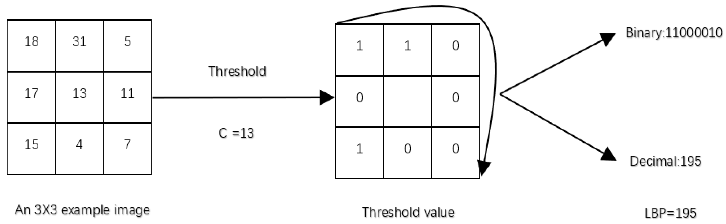
Local Binary Pattern (LBP) is a simple and effective texture operator that is widely used in the field of computer vision, especially face recognition and target detection. LBP is a neighborhood operation that analyzes the grey value changes between a pixel and its neighbors, rather than following one pixel in a particular direction. The greyscale invariance, a characteristic of LBP, can effectively reduce the influence of illumination. Chowdhury et al. [21] used Co-occurrence of Binary Pattern, an improved version of LBP, to classify dense and sparse grasses, obtaining 92.72% classification accuracy. Musci et al. [
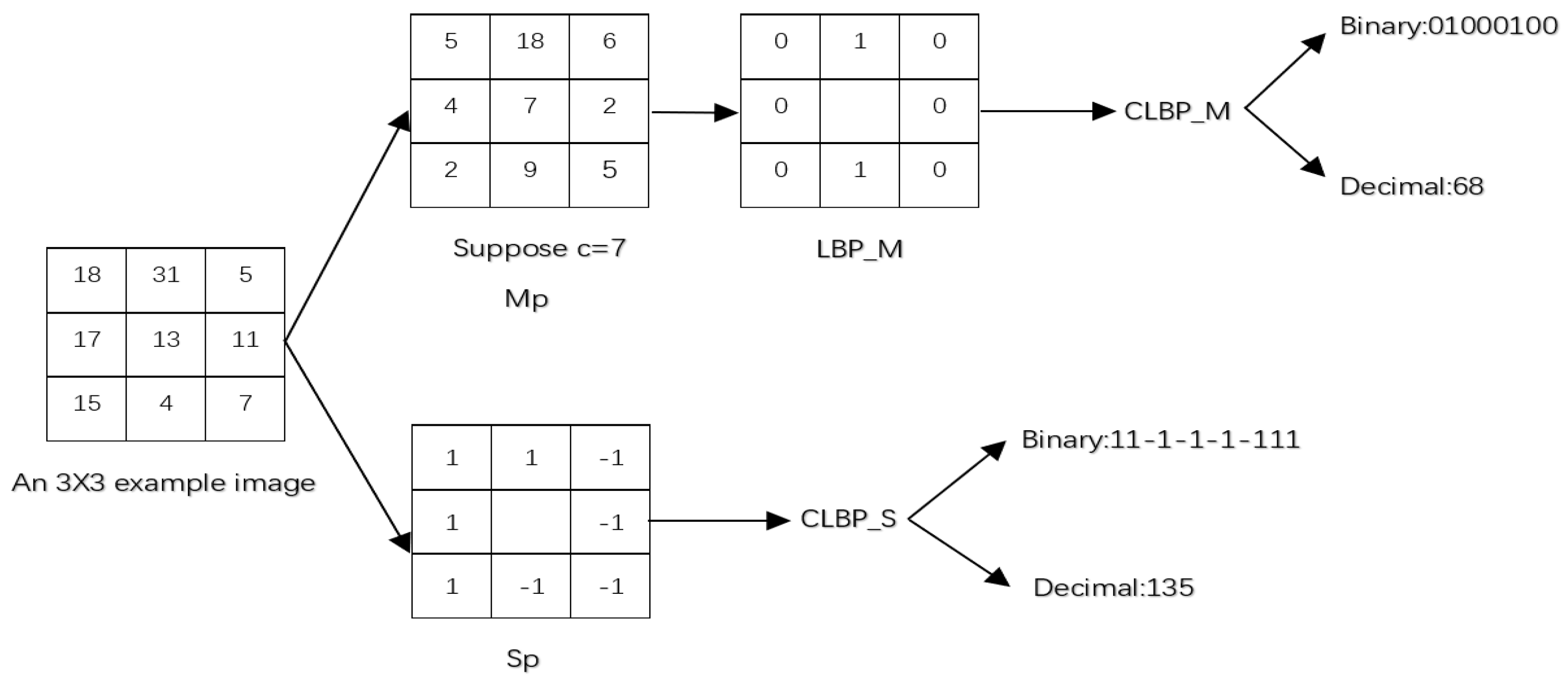
22], for their part, evaluated LBP performance in land-use/cover object-based classification of IKONOS-2 and Quickbird-2 satellite images, with the results showing that the LBP Kappa index was higher than GLCM. Since the advent of LBP, many LBP improvement algorithms have been proposed, one of which, Completed Local Binary Patterns (CLBP), takes two aspects of signs and magnitudes into account. These differences are broken down into two basic constituents, named CLBP_sign (CLBP_s) and CLBP_magnitude (CLBP_m). CLBP_s and LBP are, in fact, the same thing, just under different names. Basic constituent features can be combined through joint distributions to improve classification results. Singh et al. [23] compared CLBP to LBP in facial expression recognition, their results showing that CLBP outperformed LBP. Some other studies have also shown that the average recognition efficiency of the proposed method, using CLBP, is better than with LBP. Thus far, CLBP has not been applied in coastal wetland vegetation classification using high spatial resolution satellite images.
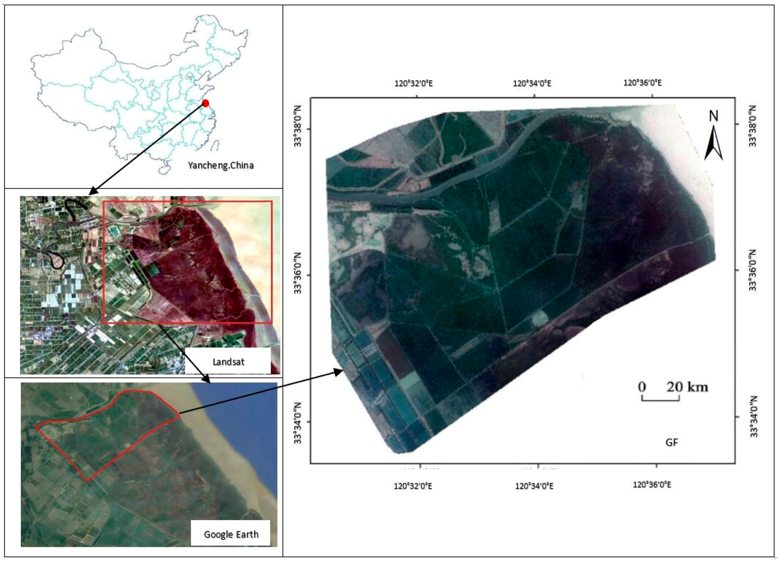
Although CLBP has been demonstrated to be superior to LBP in terms of texture analysis capabilities, our aim was to examine its performance on the classification of wetland vegetation in high spatial resolution images; accordingly, such classification was first applied based on spectrum and texture features, extracted by CLBP, via a case study of the largest tidal flat wetland in Jiangsu Province, China. The accuracy of CLBP classification was also evaluated by comparing it with GLCM.

2. Study Area and Data

2.1. Study Area

Yancheng National Natural Reservation (YNNR), the largest tidal flat wetland in China, is located in Jiangsu Province of China and stretches for 582 km along the coast of the Yellow Sea [24]. In 1992, it was approved as a National Nature Reserve by the China State Council; and in 2002, it was designated as “Ramsar Wetlands of International Importance” with the main aim of protecting shoal wetland ecosystems and rare wild animals and plants. Lying in the transition belt between the warm temperate and northern subtropical zones, YNNR is characterized by a monsoon climate. The mean annual precipitation is 980–1070 mm, while the average annual temperature is 13.7–14.6 °C [25]. The altitude in the YNNR is 0–4 m, and the terrain is dominated by a gentle slope of less than 5° [26,27]. The region has plentiful water resources and a broad marshland, which offers a natural habitat for various species of vegetation and animals. Each year, more than 300 species of migratory birds, in addition to the red-crowned crane (Grus japonensis), come here from cold northern China or other countries to stay for the long winter [26,27].
Our study was conducted in the central core zone of YNNR (Figure 1), ranging from 120°29′ E to 120°37′ E, 33°33′ N to 33°38′ N, and covering an area of 75 km2. This region comprises typical coastal salt marsh wetlands that have been well protected and managed, except for minimal human interference represented by some ditches, which are less than 20 m in width and were constructed for drainage. In addition, based on observation of Google Earth as well as field surveys, we were certain that, in the central core zone, the vegetation types are more diversified and vegetation cover is higher compared to other parts of YNNR. Thanks to its well-preserved and pristine coastal wetland vegetation, it has now been approved as one of the most important sanctuaries for the endangered red-crowned crane in China. In the area from sea to land, the stripe distribution pattern of vegetation communities is obviously caused by the plants’ succession. The main vegetation types include Spartina alterniflora, the Phragmites community, the Suaeda glauca community, and their mixture zones. A small number of trees, as well as some arable lands, are distributed throughout the study area; however, these are of negligible quantity and were not considered vegetation types. Vegetation classification, based on high spatial resolution images, is of great benefit to coastal wetland vegetation study and conservation work [28].

2.2. Data

A high spatial resolution Pléiades satellite image, acquired from Airbus Defence and Space (https://www.intelligence-airbusds.com/pleiades/), was used in this study. The cloudless, terrain-corrected images were acquired on 13 July 2015, which was a highly suitable date for vegetation identification. The images were composed of a four-band multispectral image (2 m spatial resolution) and a panchromatic band image (0.5 m spatial resolution). The wavelength characteristics of all bands are shown in Table 1. The images were registered to a Universal Transverse Mercator (UTM) projection using the World Geodetic System 1984, Zone 51. The atmosphere correction was accomplished using the FLAASH (Fast Line-of-sight Atmospheric Analysis of Spectral Hypercubes) algorithm in the Exelis Envi5.2 software [29,30].
The four-band multispectral image was fused with the panchromatic band image using the Gram-Schmit algorithm. The 0.5 m color image was obtained using the image fusion procedure. According to our previous studies [31], when it comes to vegetation classification, 0.5 m fused multispectral bands could yield a higher accuracy compared with original 2 m four bands of multispectral image and are thus more suitable. In the context of this study, fused multispectral bands were used to supply the spectrum information, and the first layer of the fused images was chosen to extract the texture features.

2.3. Field Data Collection and Sample Dataset Construction

In the previous inventory conducted by the Sheyang County Forestry Bureau, some samples were collected to provide information that was used for classification training and validation. However, further samples were collected in a field survey done in collaboration with said bureau from June to July 2017.
Because of wetland protection, the central coastal wetland is unreachable, and therefore, field surveys can only be carried out along the periphery or certain narrow roads. The surveying location on the image was recorded using GPS (Global Positioning System). Due to the limitation of segmentation objects used for training, it is hard to distinguish in the image, the homogeneous vegetation quadrant areas (e.g., more than 10 m × 10 m) were plotted on the image via visual interpretation, and thus these central points of the vegetation quadrants were sampled as field data points. As a result, 150 points were used for training samples, while 200 points were used for validation. Figure 2 shows the five vegetation classes in the visual interpretation images, as well as the photographs with their characteristics.

2.4. Texture Feature Extraction

LBP was proposed by Ojala et al. [32] for the purpose of texture classification. It works by setting a neighborhood threshold with the grey level of the central pixel as below:
L B P P , R = p = 0 P 1 s ( g p g c ) 2 p s ( x ) = { 1 , x 0 0 , x < 0
where gc represents the grey value of the center pixel and gp (p = 0, 1, …, P − 1) corresponds to the neighboring pixels selected on the circle of radius R (R > 1) and the total number of the neighbors P (P > 1). The LBPP,R value can be calculated by assigning a binomial factor 2p for each gp reassigned to the value. The LBP encoding process is illustrated in Figure 3.
As LBP is popularized, researchers have been working on the improvement of this method, for example, CLBP as proposed by Guo et al. [33]. The difference between CLBP and LBP is that CLBP does not simply assign 0 or 1 to gp, depending on gpgc. CLBP calculates the difference between gc and gp as dp = gpgc, which is the same as LBP. However, CLBP can further decompose dp into two components Sp and Mp:
d p = s p * m p   a n d   { s p = s i g n ( d p ) m p   = | d p |
where s p = { 1 , d p 0 1 , d p < 0 is the sign of dp and mp is the magnitude of dp. CLBP_s can be calculated by assigning a binomial factor 2p for each sp reassigned to the value. CLBP_m operator is defined as follows:
C L B P _ M P , R = p = 0 P 1 t ( m p , c ) 2 p , t ( x , c ) = { 1 , x c 0 , x < c
where c is the mean value of mp for the whole image.
CLBP_c is defined by converting the center pixels into a binary code using the threshold value:
C L B P _ C = t ( g c , c 1 )
where gc is set as the center pixel and c1 is the average of the whole pixels’ values.
The CLBP_m, CLBP_s, and CLBP_c represent the original image, which is combined to form the CLBP feature map (Figure 4). CLBP_m and CLBP_s could be combined to CLBP_m/s by joint histogram. Similar to the CLBP_m/s, others CLBP texture features can be setup. In this study, we chose the two CLBP texture features, CLBP_m/s and CLBP_m/s/c, which were the best results in Guo et al. [33].
GLCM was first proposed by Haralick, and is one of the best-known tools for texture analysis and extraction of spatial features in the image processing of remotely sensed data. GLCM calculates the co-occurrence matrix and obtains characteristic parameters that can reflect the changing extent of uniformity, variation, and similarity degree, with regard to directions and intervals. Before the calculation, the number of grey levels needs to be specified to simplify the calculation. The pixel of interest and its neighbor intervals of a certain distance and angle were then observed. Finally, GLCM is constructed by counting the numbers of instances of all possible neighborhoods.

2.5. Texture Feature Parameters

To compare the efficacy of the two methods, we attempted to find the most appropriate parameters for classification to enhance the results’ accuracy. We tested texture parameters using different vegetation types of sample points’ separability based on Jeffries-Matusita distance (J-M distance). The J-M distance is considered more suitable for expressing the separability characteristics of categories than other separation indicators [34]. The value of J-M distance is between 0 and 2; the larger the value, the better the separability obtained.

2.6. Image Segmentation

After analysis of the appropriate parameters, the image is segmented for classification; this is a fundamental and crucial step. In this study, a method of multi-resolution segmentation (MRS) was applied. It is a bottom-up image segmentation approach, beginning with pixel-sized objects, in which individual pixels are merged into objects based on parameters such as scale, color, shape and so on by iteration [35]. These parameters are then weighted together to define a non-overlapping homogeneity criterion, which is equivalent to a threshold, to stop object mergence. The user can control the weighting and influence the result of the image segmentation.
Scale parameter defines the maximum standard of controlling the object size. The higher the value, the larger the resulting image objects are. Scale parameter is thought as the most important parameter because the scale value influences the results of classification accuracy directly. An appropriate scale value can clearly distinguish the different objects. Smaller scale parameter values result in smaller and more image objects, increasing the classification complexity, while larger values lead to increase error classification of pixels.
In theory, the optimum scale could be determined based on internal heterogeneity threshold of the segmented object. In practice, it is suggested that the scale could be obtained by the visual inspection or quantified analysis through comparing with actual characteristics of sampling objects, for example, shape, size or the homogeneity [36]. In our study, due to the small difference of vegetation texture features in the image, it is hard to plot some sample objects for the optimum scale quantified analysis. Therefore, the optimum scale was obtained by the visual inspection of the segmented objects. In the study area, wetland vegetation types are simple, and their locations are obvious stripe distribution patterns from sea to land. As a result, the larger size scale is more suitable for systematic trial comparison. As shown in Table 2, water could be well segmented with other classes at scale 600, Phragmites at scale 300, and Spartina alterniflora, Suaeda glauca, mixed areas of vegetation and ground at scale 200. When the scales were smaller than these values in Table 2, the objects would be over-segmented [37]. For example, if the image were segmented at scale 190, the simple objects would be over-segmented into a greater number of smaller fragments. If compared with urban vegetation classification, the size of the segmentation scale is much larger than the simple vegetation spatial distribution pattern [37].
Color and shape parameters control the spectral homogeneity and texture homogeneity of the resulting image objects, respectively. Shape parameter is made up of compactness parameter and smoothness parameter [36]. The two parameters are considered as the overall compactness and smooth border, respectively. In this study, the appropriate values for individual parameters were selected in image segmentation by trial and previous experiences [31]. Table 2 shows the values of segmentation parameters used in study.

2.7. Object-Based Classification

Two kinds of sampling points were selected through fieldwork and imagery interpretation, of which 150 points were used as training points for classification, while 200 points were used as validating points for accuracy evaluation. Support Vector Machine (SVM) algorithm [37] was applied to classify the image based on the vegetation types.
SVM is a supervised classification method that overcomes the limitation of insufficient samples and reduces the effect of noisy ones. This method is a convex quadratic optimization problem, by which the global optimal solution for solving the whole equation is transformed into finding the local solution that could be accomplished by solving kennel function. The central issue for SVM is to determine hyperplane by solving the kennel function. Training data pixels closest to the hyperplane are called support vectors, which are the critical for the pixels value gap between the classes. SVM separates the image with the hyperplane that could maximize the gap between the classes. The kennel function could be linear, Polynomial, Radial Basis Function, or Sigmoid [37].
In this study, Radial Basis Function was used to determine the hyperplane, and the c parameter was set to 2. All the classifications were classified in three levels based on image segmentation, and the details for each classification are shown in Table 3.
The evaluation of classification accuracy will be carried out by a confusion matrix. The validation samples were produced based on the validation points. When more than one point was located in the same object, only one of them would be retained for the evaluation calculator.

3. Experimental Results and Discussion

3.1. Texture Parameter Selection

In this study, we calculated GLCM parameters based on two factors: texture features and window sizes. Texture features, such as Mean, Variance, Angular Second Moment (ASM), Entropy, and Contrast, were tested in the same window size. It was found that Mean ASM and Entropy were superior to the vegetation classification. Our results show that the 7*7 window size obtained the highest separability of vegetation types if compared with those of the texture features of Mean ASM and Entropy in 3 × 3, 5 × 5, and 9 × 9 window sizes.
Similarly, we selected the CLBP size and used three sizes (e.g., CLBP8,1, CLBP16,2, and CLBP24,3) to calculate the vegetation separability of CLBP’s basic elements: CLBP_m and CLBP_s. Our results show that CLBP achieved the highest separability when P = 24 and R = 3. Table 3 and Table 4 display the separability results for GLCM 7 × 7 and CLBP24,3.

3.2. Classification Results and Discussion

Object-based classification was adopted to classify spectrum alone, spectrum plus GLCM texture features, and spectrum plus CLBP texture features. Figure 5 shows classification results, with the differences of classification results between the six applied methods. The figure also shows that similar classified results were obtained for most parts of the wetland using the six methods, while some difference existed at the mixed areas of two vegetation types. Compared with the field work in Section 2.3, some areas in Figure 5 were misclassified as Suaeda glauca. It was found that the distribution of Phragmites communis was similar in different methods (see Figure 5), because this type of vegetation occupied a large area and there were no other plants interfered.
In addition, it is noted that there is an obvious stripe distribution pattern of vegetation communities, which indicates different characteristics between different types of vegetation. However, there were misclassified pixels in some small areas marked in white circles in Figure 5, which may imply that the areas are a mixture of complex vegetation or of vegetation in different growing stages. The results also show that there are some differences in the mixed vegetation communities using different texture features. These differences still need to be further studied in the future.

3.2.1. Classification Results Using Spectral Data Alone

Table 5 shows a confusion matrix for accuracy assessment using spectral information alone.
Table 5 shows that the overall 76.27% accuracy of vegetation classification is acceptable without the assistance of texture features. The error classification mainly occurred in places where the vegetation composition is complicated, such as the Phragmites communis in different growing stages or mixed with ground, or Suaeda glauca community mixed with other types. This complication leads to the misclassification of Phragmites communis to Spartina alterniflora or of Suaeda glauca with vegetation mixture areas (PC & SG or SA & SG).
As water has distinctive reflection features compared with classes, it could be discriminated from vegetation and ground in high accuracy except for some shallow water areas. Most ground areas mixed with Suaeda glauca were misclassified as vegetation. The wrong classification of ground as Suaeda glauca is the main reason of overall accuracy reduced in the study.

3.2.2. Classification Results by GLCM Texture Features

Table 6 is the confusion matrix for accuracy evaluation of vegetation classification by combining GLCM texture features with spectral information.
Table 6 shows that the overall accuracy of vegetation classification improved about 6.50% from 76.27% to 82.87% with the additional use of GLCM texture features.
Phragmites communis was managed by human activities in the study area and was distributed in aggregation. The texture of most Phragmites communis on the Pléiades satellite image is finer than any other vegetation. If Phragmites communis is mixed with Suaeda glauca, the texture will become coarser. Most mixture areas of PC & SG appear graininess features, which is helpful for improving the accuracy of vegetation classification. In the growing stage of Suaeda glauca, the image textures of Suaeda glauca or SA & SG mixture areas are coarse and chaotic.
It is obvious that the GLCM method could extract these texture characteristics at certain degree and increased about 6.50% the classification accuracy of vegetation types. The result is similar to those of previous studies in other areas [18,19].

3.2.3. Classification Results by Combining CLBP Texture Features

Table 7 is the accuracy evaluation results of vegetation classification using spectral data combined with CLBP texture features. From Table 7, it is clear that the combination of CLBP measures with spectral information improved the overall accuracy to 84.27% for CLBP_s, 85.00% for CLBP_m, 85.31% for CLBP_s/m, and 85.38% for CLBP_s/m/c, respectively, from 76.27% for spectral information alone (see Table 5). The results also indicate that additional use of CLBP texture features increased the vegetation classification accuracy of more than 8.00% in this case study.
Spartina alterniflora is another type for which the classification accuracy was highly improved by adding CLBP texture features. Spartina alterniflora is always located along the seaside, with a coarser texture on the image than Phragmites communis and Suaeda glauca. CLBP, especially CLBP_m, was better for discriminating SG than SA&SG. It improved producer accuracy by about 16.64% from 73.68% to 90.32% and user accuracy by about 20.32% from 70.00% to 90.32% (see Table 5 and Table 7).
In comparison, wrong classification can be found in the mixture areas of ground and Suaeda glauca, leading to decrease the accuracy of classification for ground and Suaeda glauca. It is noted that CLBP did not help improve classifying the mixed areas of two vegetation types, which is similar to the result in Song’s study [38]. This means that CLBP is sensitive to texture changes in producing wrong classifications of high spatial resolution images.
In addition, it is found that CLBP_m obtained high and consistent classification for vegetation types as shown in Table 7 and Figure 5. The results indicate that CLBP_m is better than other CLBP measures for classifying Phragmites communis and Suaeda glauca, above 90%, in that they are regular graininess textures, except for ground and mixed vegetation types.
When comparing Table 7 with Table 6, it is noted that the overall accuracy classification of CLBP is slightly better (2–3%) than that of GLCM. But CLBP improved classification accuracy for Spartina alterniflora 10% more than using GLCM, from 78.57% to above 90% (see Table 6 and Table 7).
Compared with the results of CLBP24,3 in Guo et al. [33] and CLBP8,1 in Dubey and Jalal [39], our overall accuracy is about 85%, which is a little bit lower than that in previous studies [33,39]. One reason might be that those researchers used CLBP in Outex database and digital imaging, while we applied it in high spatial resolution satellite images. In our view, CLBP has great potential on large-scale images such as high spatial resolution Pléiades satellite images, although the accuracy was reduced when compared to digital camera images in other studies.
Although our experiment yielded the expected results of about 85%, the study still had limitations. Most points from the field were close to the edge of the vegetation community; it is hard to reach the heart of the community because of the natural environment. If more points can be collected, including the center of the community, the accuracy of classification would be more convincing. Additionally, we chose the CLBP operator, which was more effective in Guo et al.’s study [33]. Since CLBP_c was not considered as a fundamental element, it was not discussed separately. However, CLBP_c improved the classification accuracy, whether in this study or in Guo et al. [33]. Therefore, the mechanism and effect of CLBP_c should be addressed in further studies.

4. Conclusions

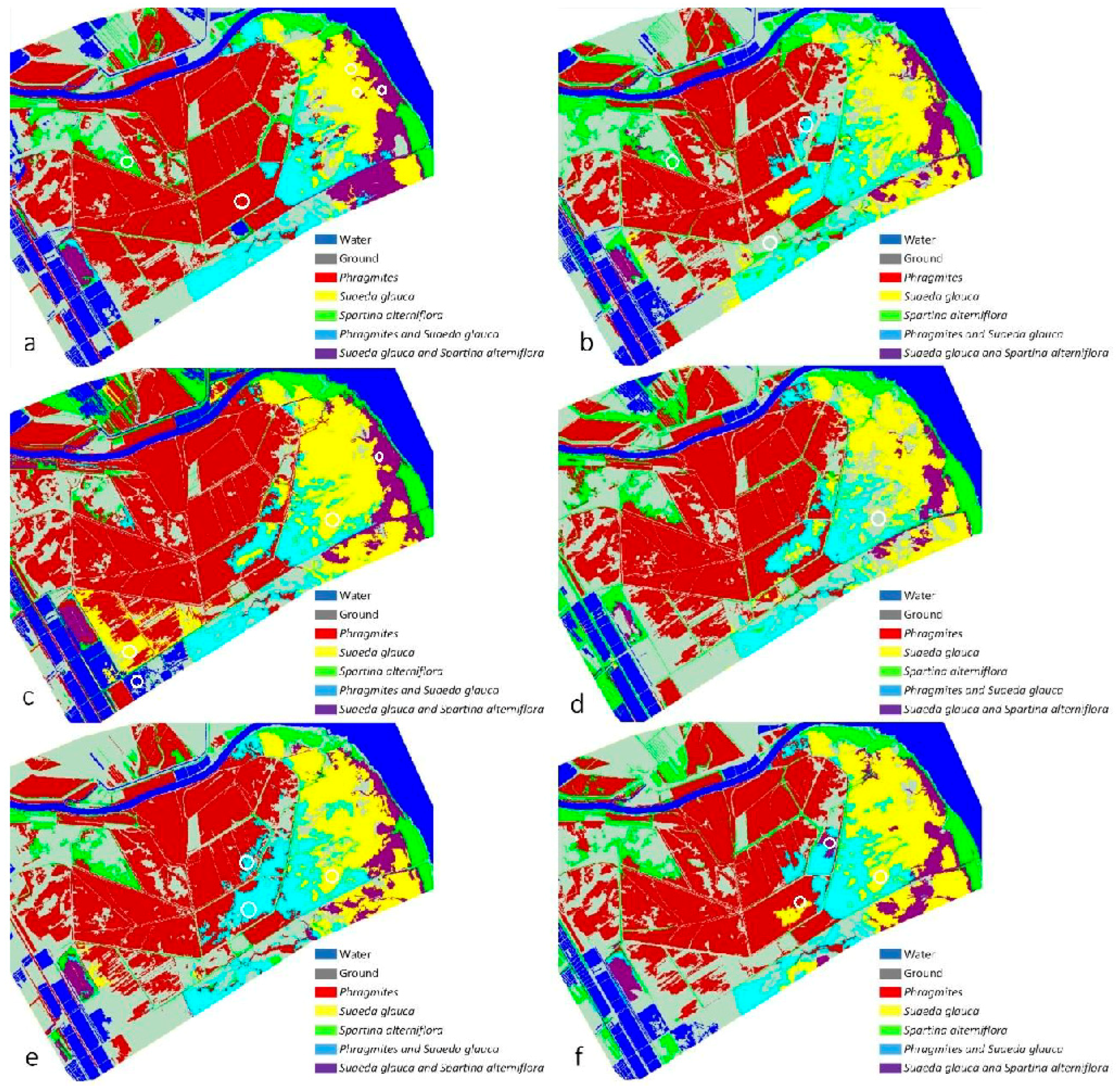
This study presented a performance assessment of texture features for the classification of coastal wetland vegetation from high spatial resolution imagery using CLBP. Based on the experimental results, it was found that both the CLBP and GLCM texture features improved classification accuracy effectively. The overall accuracy using CLBP was slightly better than with GLCM when combining spectral information with texture features. However, if comparing these vegetation classes, CLBP exhibits a better classification accuracy for Spartina alterniflora than when using GLCM. Thus, CLBP measures could be more suitable for extracting the details and regular graininess textures.
Among the various CLBP features, CLBP_m showed more effective improvement for vegetation classification, although the overall accuracy of the classification may be slightly different, including water and ground areas. However, jointed features, such as CLBP_s/m and CLBP_s/m/c, did not show greater advantages compared to CLBP_m for the mixture and complex vegetation classes.
In short, the study demonstrates that CLBP, an efficient and simple texture feature extraction method usually used in face recognition, could be applied to high spatial resolution Pléiades satellite images to classify coastal wetland vegetation. Our results evince that CLBP appears to be a promising method with regard to image classification of remote sensing data, especially in coastal wetland vegetation classification. Further research should be focused on mixed vegetation classification by refining the algorithm and attempting to combine CLBP with GLCM.

Author Contributions

X.F. and Y.Z. conceived and designed the experiments; M.W., Z.C., and X.W. performed the experiments; M.W. analyzed the data; X.F., X.L., and D.L. improved the data analysis; J.Y.T. contributed reagents/materials/analysis tools; X.F. and Y.Z. wrote the paper.

Acknowledgments

Pléiades satellite imagery data is highly appreciated. This research is jointly supported by the National Key Research and Development Program of China (Project Ref. No. 2016YFB0501501), the Natural Science Foundation of China (NSFC No. 31270745; No. 41506106), Lianyungang Land and Resources Project (LYGCHKY201701), Lianyungang Science and Technology Bureau Project (SH1629), the Priority Academic Program Development of Jiangsu Higher Education Institutions (PAPD), and the Top-notch Academic Programs Project of Jiangsu Higher Education Institutions (TAPP).

Conflicts of Interest

The authors declare no conflict of interest.

References

  1. Gorham, E. Northern peatlands: Role in the carbon cycle and probable responses to climatic warming. Ecol. Appl. 1991, 1, 182–195. [Google Scholar] [CrossRef] [PubMed]
  2. Gibbs, J.P. Wetland loss and biodiversity conservation. Conserv. Biol. 2000, 14, 314–317. [Google Scholar] [CrossRef]
  3. Wright, C.; Gallant, A. Improved wetland remote sensing in Yellowstone national park using classification trees to combine tm imagery and ancillary environmental data. Remote Sens. Environ. 2007, 107, 582–605. [Google Scholar] [CrossRef]
  4. Mutanga, O.; Adam, E.; Cho, M.A. High density biomass estimation for wetland vegetation using worldview-2 imagery and random forest regression algorithm. Int. J. Appl. Earth Obs. Geoinf. 2012, 18, 399–406. [Google Scholar] [CrossRef]
  5. Maclean, I.; Hassall, M.; Boar, R.R.; Lake, I.R. Effects of disturbance and habitat loss on papyrus-dwelling passerines. Biol. Conserv. 2006, 131, 349–358. [Google Scholar] [CrossRef]
  6. Mafabi, P. The role of wetland policies in the conservation of waterbirds: The case of uganda. Ostrich 2000, 71, 96–98. [Google Scholar] [CrossRef]
  7. Owino, A.O.; Ryan, P.G. Recent papyrus swamp habitat loss and conservation implications in western Kenya. Wetl. Ecol. Manag. 2007, 15, 1–12. [Google Scholar] [CrossRef]
  8. Liu, C.Y.; Jiang, H.X.; Hou, Y.Q.; Zhang, S.Q.; Su, L.Y.; Li, X.F.; Pan, X.; Wen, Z. Habitat changes for breeding waterbirds in Yancheng National Nature Reserve, China: A remote sensing study. Wetlands 2010, 30, 879–888. [Google Scholar] [CrossRef]
  9. Zhang, Y.; SUN, Y.; Lu, C.H.; Zhang, Y.L.; Lv, S.C. Pattern of Wintering Bird Community in Three Habitats after Invasion of Spartina alterniflora in Yancheng National Nature Reserve. Wetl. Sci. 2017, 15, 433–441. [Google Scholar]
  10. Tan, Q.; Liu, H.; Zhang, H.; Wang, C.; Hou, M. Classification of vegetation coverage of wetland landscape based on remote sensing in the coastal area of Jiangsu Province. Remote Sens. Technol. Appl. 2013, 28, 934–940. [Google Scholar]
  11. Liu, X.; Xu, M. Beach vegetation ecological character in north Jiangsu shoal of east china and its succession. J. Nanjing Norm. Univ. 2015, 38, 107–113. [Google Scholar]
  12. Simard, M.; Saatchi, S.S.; De Grandi, G. The use of decision tree and multiscale texture for classification of JERS-1 SAR data over tropical forest. IEEE Trans. Geosci. Remote Sens. 2000, 38, 2310–2321. [Google Scholar] [CrossRef]
  13. Yu, Q.; Gong, P.; Clinton, N.; Biging, G.; Kelly, M.; Schirokauer, D. Object-based detailed vegetation classification with airborne high spatial resolution remote sensing imagery. Photogramm. Eng. Remote Sens. 2006, 72, 799–811. [Google Scholar] [CrossRef]
  14. Maillard, P. Comparing texture analysis methods through classification. Photogramm. Eng. Remote Sens. 2003, 69, 357–367. [Google Scholar] [CrossRef]
  15. Beguet, B.; Chehata, N.; Boukir, S.; Guyon, D. Classification of forest structure using very high resolution Pleiades image texture. In Proceedings of the 2014 IEEE International Geoscience and Remote Sensing Symposium, Quebec City, QC, Canada, 13–18 July 2014; Volume 2014, pp. 2324–2327. [Google Scholar]
  16. Szantoi, Z.; Escobedo, F.J.; Abd-Elrahman, A.; Pearlstine, L.; Dewitt, B.; Smith, S. Classifying spatially heterogeneous wetland communities using machine learning algorithms and spectral and textural features. Environ. Monit. Assess. 2015, 187, 1–15. [Google Scholar] [CrossRef] [PubMed]
  17. Cabezas, J.; Galleguillos, M.; Perez-Quezada, J.F. Predicting vascular plant richness in a heterogeneous wetland using spectral and textural features and a random forest algorithm. IEEE Geosci. Remote Sens. Lett. 2016, 13, 646–650. [Google Scholar] [CrossRef]
  18. Berberoğlu, S.; Akin, A.; Atkinson, P.M.; Curran, P.J. Utilizing image texture to detect land-cover change in Mediterranean coastal wetlands. Int. J. Remote Sens. 2010, 31, 2793–2815. [Google Scholar] [CrossRef]
  19. Arzandeh, S.; Wang, J. Texture evaluation of Radarsat imagery for wetland mapping. Can. J. Remote Sens. 2002, 28, 653–666. [Google Scholar] [CrossRef]
  20. Kamarul, H.G.; Aini, H. Machine vision system for automatic weeding strategy using image processing technique. Am.-Eurasian J. Agric. Environ. Sci. 2008, 3, 451–458. [Google Scholar]
  21. Chowdhury, S.; Verma, B.; Stockwell, D. A novel texture feature based multiple classifier technique for roadside vegetation classification. Expert Syst. Appl. 2015, 42, 5047–5055. [Google Scholar] [CrossRef]
  22. Musci, M.; Feitosa, R.Q.; Velloso, M.L.F.; Novack, T. An evaluation of texture descriptors based on local binary patterns for classifications of remote sensing images. Bol. Cienc. Geodesicas 2011, 17, 549–570. [Google Scholar]
  23. Singh, S.; Maurya, R.; Mittal, A. Application of Complete Local Binary Pattern Method for facial expression recognition. In Proceedings of the International Conference on Intelligent Human Computer Interaction, Kharagpur, India, 27–29 December 2012; Volume 2013, pp. 1–4. [Google Scholar]
  24. Xu, H.; Zhu, G.Q.; Wang, L.; Bao, H. Design of nature reserve system for red-crowned crane in china. Biodivers. Conserv. 2005, 14, 2275–2289. [Google Scholar] [CrossRef]
  25. Wang, J.; Liu, Z. Protection and sustainable utilization for the biodiversity of Yancheng seashore. Chin. J. Ecol. 2005, 24, 1090–1094. [Google Scholar]
  26. Lu, Y. The Role of Local Knowledge in Yancheng National Nature Reserve Management. Ph.D. Thesis, University of Otago, Dunedin, New Zealand, 2016. [Google Scholar]
  27. Ke, C.Q. Analyzing coastal wetland change in the Yancheng National Nature Reserve, China. Reg. Environ. Chang. 2011, 11, 161–173. [Google Scholar] [CrossRef]
  28. Sun, J.; Han, L.J.; Sun, D.Y.; Yuan, Z.H. The studies on anti-drought of seaweed extracts. Mar. Sci. 2006, 30, 40–45. [Google Scholar]
  29. Cooley, T.; Anderson, G.P.; Felde, G.W.; Hoke, M.L. FLAASH, a MODTRAN4-based atmospheric correction algorithm, its application and validation. In Proceedings of the 2002 IEEE International Geoscience and Remote Sensing Symposium (IGARSS ’02), Toronto, ON, Canada, 24–28 June 2002; pp. 1414–1418. [Google Scholar]
  30. Cheng, L.; Youhua, M.A.; Huang, Y.; Zhi, X.; Juan, Z.U.; Zhongwen, M.A. Comparison of atmospheric correction between ENVI FLAASH and ERDAS ATCOR2. Agric. Netw. Inf. 2011, 12, 007. [Google Scholar]
  31. Wang, M.Y.; Fei, X.Y.; Xie, H.Q.; Liu, F.; Zhang, H. Study of Fusion Algorithms with High Resolution Remote Sensing Image for Urban Green Space Information Extraction. Bull. Surv. Mapp. 2017, 36–40. [Google Scholar] [CrossRef]
  32. Ojala, T.; Pietikäinen, M.; Harwood, D. A comparative study of texture measures with classification based on feature distributions. Pattern Recognit. 1996, 29, 51–59. [Google Scholar]
  33. Guo, Z.; Zhang, L.; Zhang, D. A completed modeling of local binary pattern operator for texture classification. IEEE Trans. Image Process. 2010, 19, 1657–1663. [Google Scholar] [PubMed]
  34. Bruzzone, L.; Roli, F.; Serpico, S.B. An extension of the Jeffreys-Matusita distance to multiclass cases for feature selection. IEEE Trans. Geosci. Remote Sens. 1995, 33, 1318–1321. [Google Scholar] [CrossRef]
  35. Duro, D.C.; Franklin, S.E.; Dubé, M.G. A comparison of pixel-based and object-based image analysis with selected machine learning algorithms for the classification of agricultural landscapes using SPOT-5 HRG imagery. Remote Sens. Environ. 2012, 118, 259–272. [Google Scholar] [CrossRef]
  36. Wulder, M.A.; Chubey, M.S.; Franklin, S.E. Object-based analysis of ikonos-2 imagery for extraction of forest inventory parameters. Photogramm. Eng. Remote Sens. 2006, 72, 383–394. [Google Scholar]
  37. Mountrakis, G.; Im, J.; Ogole, C. Support vector machines in remote sensing: A review. ISPRS J. Photogramm. Remote Sens. 2011, 66, 247–259. [Google Scholar] [CrossRef]
  38. Song, B.Q.; Li, P.J. The application of extended lbp texture in high resolution remote sensing image classification. Remote Sens. Land Resour. 2010, 25, 40–45. [Google Scholar]
  39. Dubey, S.R.; Jalal, A.S. Detection and Classification of Apple Fruit Diseases Using Complete Local Binary Patterns. In Proceedings of the Third International Conference on Computer and Communication Technology, Allahabad, India, 23–25 November 2012; IEEE Computer Society: Washington, DC, USA, 2012; pp. 346–351. [Google Scholar]
Figure 1. The location of the study area.
Remotesensing 10 00778 g001
Figure 2. The vegetation types for classification and their image characteristics.
Remotesensing 10 00778 g002
Figure 3. An example of encoding process of LBP (P = 8, R = 1).
Remotesensing 10 00778 g003
Figure 4. An example of encoding process of CLBP_s and CLBP_m (P = 8, R = 1).
Remotesensing 10 00778 g004
Figure 5. Classification results: (a) Spectral textures; (b) Spectral and GLCM textures; (c) Spectral and CLBP_S textures; (d) Spectral and CLBP_M textures; (e) Spectral and CLBP_M/S textures; and (f) Spectral and CLBP_M/S/C textures.
Remotesensing 10 00778 g005
Table 1. Pléiades Band Descriptions.
BandWavelength (nm)Spectral Region
1430–550Blue
2490–610Green
3600–720Red
4750–950Near Infrared
Table 2. Segmentation parameters and optimum segmented images used in this study.
Objects (Scale)Optimum Segmented ImagesColor/ShapeSmoothness/CompactnessFeatures
Water (600) Remotesensing 10 00778 i0010.9/0.10.5/0.5The features used to perform image segmentation correspond to each procedure of classification
Phragmites (300) Remotesensing 10 00778 i002
Mixed Spartina alterniflora and Suaeda glauca (200) Remotesensing 10 00778 i003
Table 3. Vegetation separability in the window size of GLCM 7 × 7.
Separability of Mean Texture Feature
ClassesPCSASGPC & SGSA & SG
PC
SA2.000
SG1.9852.000
PC & SG1.9991.9451.992
SA & SG1.9051.9360.8111.564
Separability of ASM Texture Feature
PC
SA2.000
SG1.9802.000
PC & SG1.9991.9571.992
SA & SG1.9461.9210.8661.134
Separability of Entropy Texture Feature
PC
SA2.000
SG1.9802.000
PC & SG1.9991.9531.992
SA & SG1.9651.9210.9411.136
Table 4. Vegetation separability in the window size of CLBP24,3.
Separability of CLBP_M
ClassesPCSASGPC & SGSA & SG
PC
SA2.000
SG1.9921.999
PC & SG1.9951.9371.985
SA & SG1.8961.8931.2091.571
Separability of CLBP_S
PC
SA2.000
SG1.8211.991
PC & SG1.9811.3091.987
SA & SG1.8991.9171.1181.562
Note: PC represents Phragmites communis. SA is Spartina alterniflora and SG means Suaeda glauca community. PC & SG indicates the mixed vegetation of Phragmites communis and Suaeda glauca, While SA & SG is the mixed vegetation of Spartina alterniflora and Suaeda glauca.
Table 5. Confusion matrix of classification by spectral data.
WaterGroundPCSASGPC & SGSA & SGSumUser Accuracy
Water173000012180.95%
Ground026012203183.87%
Pc013030103585.71%
SA010140232070.00%
SG023018232878.57%
PC & SG016011512479.17%
SA & SG010110151883.33%
Sum17353919222223177
Producer Accuracy100.00%74.29%76.92%73.68%81.82%68.18%65.22%
Overall Accuracy = 76.27%
Note: PC represents Phragmites communis. SA is Spartina alterniflora and SG means Suaeda glauca community. PC & SG indicates the mixed vegetation of Phragmites communis and Suaeda glauca, While SA & SG represents the mixed vegetation of Spartina alterniflora and Suaeda glauca.
Table 6. Confusion matrix of classification by spectral data and GLCM.
WaterGroundPSASGPC & SGSA & SGSumUser Accuracy
Water243000012885.71%
Ground125012023180.65%
P012720203284.38%
SA020220222878.57%
SG001026123081.25%
PC & SG010111301673.33%
SA & SG010200131681.25%
Sum25332828291820181
Producer Accuracy96.00%75.76%96.43%78.57%89.66%72.22%65.00%
Overall Accuracy = 82.87%
Note: PC represents Phragmites communis. SA is Spartina alterniflora and SG means Suaeda glauca community. PC & SG indicates the mixed vegetation of Phragmites communis and Suaeda glauca, While SA & SG represents the mixed vegetation of Spartina alterniflora and Suaeda glauca.
Table 7. Confusion matrix of classification by spectral data and CLBP.
WaterGroundPSASGPC & SGSA & SGSumUser Accuracy
SWater192000012286.36%
Ground021002222777.77%
P003610203989.74%
SA010210132680.77%
SG001025223086.67%
PC & SG001011211585.71%
SA & SG010110161984.21%
Sum19253823291925178
Producer Accuracy100.00%84.00%94.74%91.30%86.21%63.16%64.00%
Overall Accuracy = 84.27%
WaterGroundPSASGPC & SGSA & SGSumUser Accuracy
MWater162000011984.21%
Ground026003103086.67%
P003020023488.24%
SA000280123190.32%
SG031023213076.67%
PC & SG011011301681.25%
SA & SG010110172085.00%
Sum16333231281723180
Producer Accuracy100.00%78.79%93.75%90.32%82.14%76.47%73.91%
Overall Accuracy = 85.00%
WaterGroundPSASGPC & SGSA & SGSumUser Accuracy
M/SWater193000012382.61%
Ground124011123080.00%
P013310303886.41%
SA010270123187.10%
SG001023022688.46%
PC & SG001101301586.67%
SA & SG000002121485.71%
Sum20293530241821177
Producer Accuracy95.00%82.76%94.29%90.00%95.83%72.22%57.14%
Overall Accuracy = 85.31%
WaterGroundPSASGPC & SGSA & SGSumUser Accuracy
S/M/CWater182000012185.71%
Ground122001122781.48%
P012910303485.29%
SA010240122885.71%
SG000024112692.37%
PC & SG003011512075.00%
SA & SG000100141593.33%
Sum19263226262221171
Producer Accuracy94.74%84.62%90.63%92.31%92.31%68.18%66.67%
Overall Accuracy = 85.38%
Note: PC represents Phragmites communis. SA is Spartina alterniflora and SG means Suaeda glauca community. PC & SG indicates the mixed vegetation of Phragmites communis and Suaeda glauca, While SA & SG represents the mixed vegetation of Spartina alterniflora and Suaeda glauca.

