Dynamic Monitoring and Vibration Analysis of Ancient Bridges by Ground-Based Microwave Interferometry and the ESMD Method

1
Key Laboratory for Urban Geomatics of National Administration of Surveying, Mapping and Geoinformation, Beijing Key Laboratory for Architectural Heritage Fine Reconstruction & Health Monitoring, Beijing University of Civil Engineering and Architecture, 1 Zhanlanguan Road, Beijing 100044, China
2
College of Surveying and Geo-informatics, Tongji University, 1239 Siping Road, Shanghai 200092, China
*
Authors to whom correspondence should be addressed.
Remote Sens. 2018, 10(5), 770; https://doi.org/10.3390/rs10050770
Submission received: 21 March 2018
/
Revised: 8 May 2018
/
Accepted: 14 May 2018
/
Published: 16 May 2018
Abstract
:In this paper, we propose to conduct a dynamic monitoring and vibration analysis of ancient bridges by means of ground-based microwave interferometry and the extreme-point symmetric mode decomposition (ESMD) method. Ground-based microwave interferometry, a novel non-contact technology with a high accuracy, is used to acquire dynamic time series displacements with environmental excitation factors and a transient load with a car, respectively. The ESMD method, a new alternative to the Hilbert-Huang transform (HHT), is adopted to conduct the instantaneous vibration analysis of Zhaozhou Bridge. Firstly, a series of intrinsic mode functions (IMFs) are obtained together with an optimal adaptive global mean (AGM) curve by using a mode symmetric about the maxima and minima points. Secondly, the instantaneous frequency of each IMF is obtained by the use of a direct interpolation algorithm, which can reconcile the conflict between the period and the frequency for the traditional time-frequency analysis methods. As a representative case, Zhaozhou Bridge, a well-known Chinese ancient bridge constructed more than 1400 years ago, is studied in detail. Four kinds of dynamic time series displacements—two of them acquired by considering only environmental excitation factors for the mid-span and 1/4-span points and the others obtained with the transient load of a car for the mid-span and 1/4-span points—are selected to pursue a comparison of the decomposed IMFs and the instantaneous frequencies to perform the instantaneous vibration analysis of Zhaozhou Bridge. By comparing the results obtained with HHT for the decomposed IMFs and the instantaneous frequencies, the results show that the proposed method has a powerful ability to evaluate the instantaneous dynamic response of ancient bridges.

1. Introduction
With the inevitable aging of ancient bridges, there is now an urgent problem worldwide for dynamic monitoring and vibration analysis [1]. To safeguard the stability of ancient bridges, regular inspection and analysis are essential. At present, dynamic testing under ambient excitation (usually due to traffic or wind) is the main experimental method used to acquire the dynamic responses of bridges in service, which is an approach that has attracted significant research attention [2,3]. Most of the typical experimental tests have been carried out using piezoelectric accelerometers and fiber optic sensors [4,5]. These transducers can accurately and reliably acquire dynamic time series displacements. However, they need to be fixed in specific positions on the measured bridges and require hardwiring from the transducers to the data acquisition system [6]. This is a time-consuming and expensive task and may result in some damages to the ancient bridges.
Ground-based microwave interferometry is an alternative technology for vibration measurement that has been widely applied to determine the dynamic displacement of bridges [7,8,9,10]. The great advantages of this technique include non-contact displacement measurement, a wide frequency range of responses, sub-millimetric displacement sensitivity, and quick set-up. By regarding the reflected points of the electromagnetic wave as a series of virtual sensors, the non-contact capability can strongly reduce or even nullify the use of the traditional point sensors, whose positioning involves the use of cumbersome and costly scaffolding, which is occasionally undertaken under hazardous conditions [11]. Accuracy comparisons have been made in the laboratory and on-site between ground-based microwave interferometry and the traditional transducers (such as accelerometers and seismometers), and it has been reported that ground-based microwave interferometry can achieve an accuracy of between 1/100 and 1/10 of a millimeter [11,12].
Time-frequency analysis is a commonly used method for structural damage detection by analyzing the vibration-based time series displacements directly. At present, the most widely used time-frequency analysis methods are short-time Fourier transform (STFT), wavelet analysis, and Hilbert-Huang transform (HHT). STFT is the first kind of method of time-frequency analysis, and is a Fourier-related transform used to determine the sinusoidal frequency and phase content of local sections of a signal as it changes over time. Due to the time-bandwidth product theorem, a tradeoff exists between the time and frequency resolution, which makes STFT of limited use [2]. Wavelet analysis is a representation of a function by wavelets, which are the scaled and translated copies of a finite-length or fast-decaying oscillating waveform. As wavelets can be localized in both time and frequency, they can be easily applied in the field of structural damage detection [13,14]. However, wavelet transform is still an adaptive window Fourier method based on the principle of linear superposition, can only handle non-stationary signals for linear systems, and relies on a priori knowledge [15,16]. Furthermore, the results of wavelet analysis are limited by the size of the mother wavelet.
Generally speaking, under the designed load, the dynamic responses of structures should be linear. However, non-stationary and non-linear signals often result from the ambient excitation, and these signals are difficult to process using the traditional Fourier-based methods (e.g., STFT and wavelet analysis). Therefore, a great deal of attention has been placed on analyzing non-stationary and non-linear signals in recent years. In this context, the concept of the instantaneous frequency of a signal, an oscillating change rate during the process of moving back and forth, has become very popular [2,16]. Therefore, it is appropriate to analyze the time series displacements from dynamic testing under ambient excitation for bridges. At present, a commonly acceptable definition for instantaneous frequency relies on the analytical signal obtained by the use of HHT [17]. HHT is an innovative method of adaptive time-frequency analysis, with the ability to analyze non-linear systems or non-stationary data, which is based on empirical mode decomposition (HHT-EMD) and Hilbert spectral analysis [15]. By using the HHT-EMD method, any complicated response signal can be decomposed into a series of finite and small intrinsic mode functions (IMFs), and the meaningful instantaneous frequency of each IMF can be determined and used to build the Hilbert spectrum [17]. With the advantage of requiring neither an a priori primary function nor a preset window length, HHT has been successfully applied in the field of vibration-based structural damage detection. Huang et al. [18] noted the frequency downshift as indications of structural yield by examining the Hilbert spectrum and marginal Hilbert spectrum for damage detection of a bridge pier because of piling. Roveri and Carcaterra [2] proposed to adopt a novel HHT-based method for the damage detection of bridge structures under a traveling load, and the damage location is revealed by the inspection of the first instantaneous frequency curve of the corresponding decomposed IMF. Quek et al. [19] illustrated the feasibility of HHT for locating an anomaly, in the form of a crack, delamination, stiffness loss, or boundary in beams and plates, based on physically acquired propagating wave signals. Chen et al. [20] performed a dynamic-based damage detection for large structural systems through the use of HHT, and pointed out that the instantaneous frequency of the decomposed IMFs is more sensitive to structural damage. Kunwar et al. [21] presented the health monitoring of an experimental bridge model based on transient vibration data using HHT.
Extreme-point symmetric mode decomposition (ESMD) is a new alternative to HHT proposed by Wang and Li in 2013 [16]. Differing from HHT, the ESMD method permits the residual component to possess a certain number of extreme points, without decomposing a signal to the last trend function with, at the most, one extreme point [16]. This residual component can better reflect the evolutionary trend of the whole data. In this context, it can be understood as an optimal adaptive global mean (AGM) curve, which reduces the difficulty of determining the sifting time and improves the accuracy of the decomposed IMFs [16,22]. A comparison of the HHT-EMD method and the ESMD method has been performed by decomposing a simulation signal, which consists of three sub-signals with different frequencies and white Gaussian noise, with a signal-to-noise ratio (SNR) of 10 dB. The results showed that the ESMD method performed better than the HHT-EMD method, of which the decomposed IMFs were more consistent with the above three sub-signals, and the mode mixing problems were also evidently decreased [17]. Moreover, HHT has the disadvantage of computing a meaningful instantaneous frequency, so this method requires a hypothesis that the signal itself is locally smooth and the derivative of the phase function of the input data exists [16,23]. Unfortunately, the dynamic time series displacements of bridges do not always conform to the hypothesis. In order to address this issue, the ESMD method has been adopted to determine the instantaneous frequency and amplitude in a direct interpolation approach, which utilizes the data-based direct interpolation approach to calculate the meaningful instantaneous frequency point by point in time [16,24]. Liu et al. [23] conducted a stability analysis of the progressive collapse of a building model using the ESMD method, and the results show that the obtained instantaneous frequency of each IMF can not only detect damages of a building model, but can also analyze load-bearing conditions.
The purpose of this study was to perform the instantaneous vibration analysis of ancient bridges through the use of the ESMD method based on the dynamic time series displacements. In this study, we take the ancient bridge of Zhaozhou Bridge as an experimental object, of which dynamic time series displacements were obtained by ground-based microwave interferometry (the IBIS-S instrument). Two kinds of tests were performed to acquire the dynamic time series displacements for Zhaozhou Bridge; one test was undertaken with only environmental excitation factors and the other test was undertaken with the transient load of a car weighing more than two tons. The ESMD method was adopted to yield a series of IMFs to reflect the overall tendency of the projected displacement according to the magnitude of the frequency. The direct interpolation algorithm was adopted to obtain the meaningful instantaneous frequencies of the corresponding decomposed IMFs to analyze the stability of Zhaozhou Bridge under the transient load of a car. The rest of this paper is organized as follows. Zhaozhou Bridge and the measurement method are introduced in Section 2. Section 3 introduces the ESMD method for non-linear, non-stationary data processing, including the decomposition algorithm of the ESMD method for the time series displacements and the direct interpolation algorithm for instantaneous frequency. Section 4 describes the experimental results and analysis for Zhaozhou Bridge, followed by the conclusion in Section 5.
2. Study Ancient Bridge and Data Acquisition
2.1. Zhaozhou Bridge
Zhaozhou Bridge, which is also known as Anji Bridge or Dashi Bridge, is the oldest open-spandrel stone segmental-arch bridge in the world. Credited to the design of a craftsman named Li Chun, the bridge was constructed in the Sui Dynasty, more than 1400 years ago, and is located on the Xiaohe River in Zhaozhou County, Hebei province, China. Figure 1 shows a sketch of Zhaozhou Bridge. The bridge is about 50.82 m long, with a central span of 37.47 m, which was the world’s longest arch bridge at the time of construction. The bridge stands 7.3 m tall and has a width of 9 m. The arch covers a circular segment of less than half of a semicircle (84°), with a radius of 27.27 m [25,26,27].
2.2. Ground-Based Microwave Interferometry
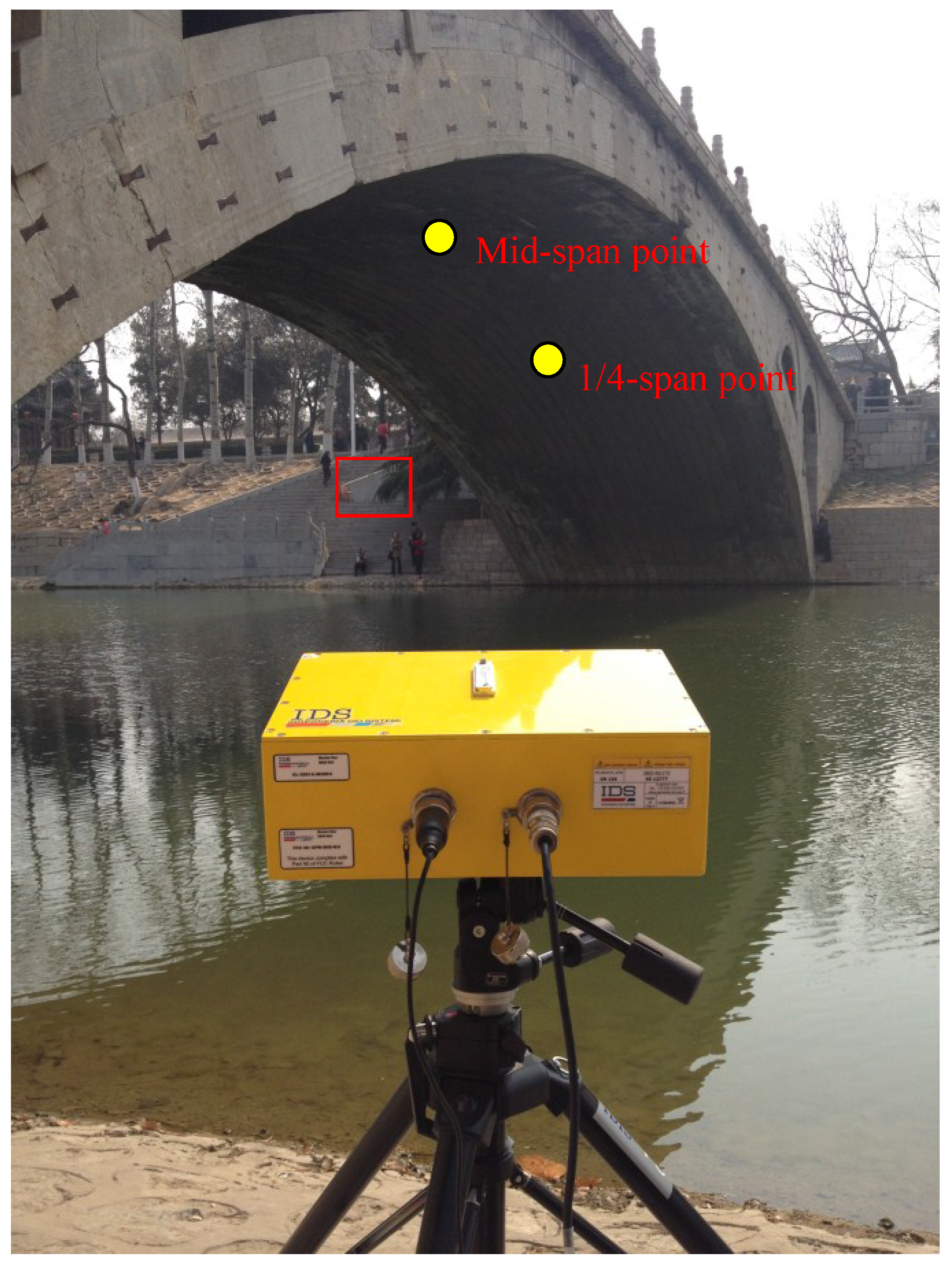
In this study, Imaging by Interferometric Survey (IBIS-S), a typical system based on ground-based microwave interferometry for the remote dynamic monitoring of structures, was adopted to acquire accurate dynamic time series displacements. The IBIS-S system was developed by the Ingegneria Dei Sistemi (IDS) Company, Pisa, Italy, in collaboration with the Department of Electronics and Telecommunications of Florence University. The IBIS-S instrument consists of a radar unit, a control PC, a power supply unit, and a tripod, with the ability of displacement monitoring in any weather conditions, independent of daylight [10]. The radar unit, a coherent sensor module, can generate, transmit, and receive the electromagnetic signals, and further process the preserved phase information of the received signals to calculate the displacement of the monitored objects. The control PC is connected to the radar unit by a standard USB 2.0 interface (Figure 2), and it can be used to configure the parameters and manage and store the measurements. It also allows the user to view the initial results of the key locations in real time [10].
The stepped-frequency continuous wave (SF-CW) and ground-based microwave interferometry are the two key technologies of the IBIS-S system.
The purpose of the SF-CW technique is to provide the capability of long-distance transmission and a higher range resolution, without the need to install multiple units on the monitored objects [28]. By using the SF-CW technique, the radar unit of the IBIS-S system transmits a set of continuous electromagnetic waves at discrete frequency values, with a sampling bandwidth and a constant interval . Therefore, the range resolution can be calculated using the corresponding continuous-wave signals by , where denotes the speed of light in a vacuum. For the IBIS-S system, the bandwidth range is 300 MHz, and thus a range resolution of up to 0.5 m can be obtained [10]. This means that each object point can be observed separately by not less than 0.5 m from another point along the radial direction [29]. Moreover, since the significant frequency content of time series displacements is in the range of 0–20 Hz for a civil engineering structure, the system is highly suited to analyzing the instantaneous dynamic response of Zhaozhou Bridge, with a sampling rate of up to 200 Hz to sample the scenario and a bandwidth of 300 MHz. In other words, the sampling interval of 0.005 s is well suited to providing a good wave definition for the acquired time series displacements [6].
Ground-based microwave interferometry is adopted to ensure a higher displacement accuracy at a high sampling rate [30]. In general, amplitude and phase information can be acquired for each measurement using ground-based microwave interferometry. Therefore, considering a single target, a tiny displacement along the radar line-of-sight direction can be calculated through comparing the phase shift at different times by , where is the length of the electromagnetic wave and is the phase shift [31]. For IBIS-S, the Ku-band of the working Radar is between 16.6–16.9 GHz, the approximate value of is 18.07 mm, the maximum value of is , and therefore, the maximum range of displacement along the radar line-of-sight direction is about 4.5175 mm for the adjacent sampling interval. However, since ground-based microwave interferometry provides a measurement of the line-of-sight displacement, it requires prior knowledge of the direction of motion to evaluate the actual displacement. For the monitored Zhaozhou Bridge in this study, the displacement under environmental excitation factors and traffic loads can be regarded as the projected displacement, which can be calculated by making straightforward geometric projections [10,28].
In summary, in typical measurement conditions, the radar unit has the following characteristics: the maximum detection distance is up to 1 km, the range resolution is up to 0.50 m, the sampling rate is up to 200 Hz, and the displacement measurement accuracy is up to 0.01 mm. However, in the practical application, the displacement measurement accuracy depends on the power of the reflected target. The general measurement accuracy is between 0.01 mm and 0.1 mm.
2.3. Dynamic Time Series Displacements Acquisition
Two kinds of tests were carried out to acquire the dynamic time series displacements for Zhaozhou Bridge with the IBIS-S instrument, for which the parameter settings are shown in Table 1. One test was undertaken with only environmental excitation factors (Test 1). In other words, no pedestrians or vehicles passed over the bridge during the data acquisition. The other test was undertaken with the transient load of a car weighing more than 2 tons (Test 2), which went back and forth over the bridge four times with a speed of about 20 km/h. For test 2, aiming to avoid any damage to Zhaozhou Bridge, only one set of time series displacements was collected to analyze the instantaneous dynamic response for Zhaozhou Bridge, of which the duration was 1 min and 47 s. For Test 1, five sets of time series displacements were collected, which have similar change tendencies. Moreover, in order to facilitate the subsequent contrast analysis, the experimental duration was between 2 and 3 min for each set. Hence, only one of the five sets of time series displacements was selected to conduct the analysis in this paper, of which the duration was 2 min and 45 s, as shown in Table 1. Obviously, the two tests employed short observation periods, so it was difficult to perform the global stability analysis for Zhaozhou Bridge. However, as the tests were more sensitive to reflecting the instantaneous stability of bridges for the instantaneous frequency of the decomposed IMFs and a high sampling rate of 199.17 Hz for the IBIS-S instrument [20], the duration of the two tests was enough to evaluate the instantaneous dynamic response of Zhaozhou Bridge, especially for Test 2 with four continuous excitations under the transient load of a car. Furthermore, in order to guarantee the uniform initial reference displacement for the two kinds of tests, the IBIS-S instrument was fixed during the two tests. As shown in Figure 1 and Figure 2, the IBIS-S instrument was located at one side of Zhaozhou Bridge. The angle of altitude of the radar unit was set to 12°, so that the two antennas on the radar unit could be aligned to the mid-span point of the central span. Considering that Zhaozhou Bridge is of great historical heritage, no corner reflectors were installed on the lower surface of the central span. The acquired time series displacements along the radar line-of-sight direction were directly calculated by the reflected microwave signal from the natural surface of the arch, which was then vertically projected to obtain the projected time series displacements [10,28].
3. Methods
The ESMD method involves two distinct steps: (1) the decomposition step to yield a series of IMFs together with an optimal adaptive global mean (AGM) curve; and (2) the direct interpolation algorithm to yield the instantaneous frequency of each IMF.
3.1. Decomposition Algorithm of the ESMD Method for Time Series Displacements
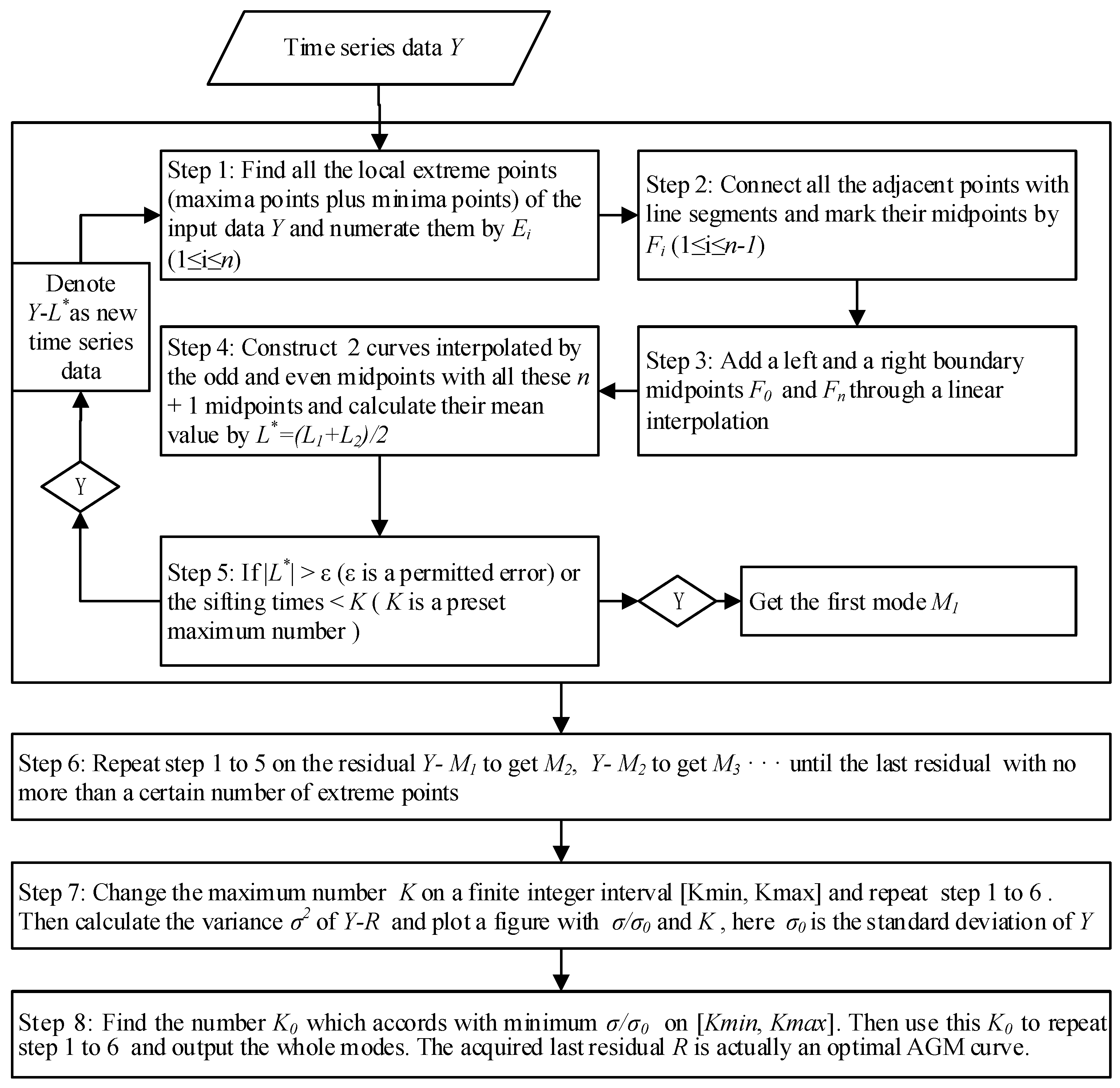
Differing from the scheme of the HHT-EMD method, i.e., making a mode symmetric about its upper and lower envelope interpolated by the local maxima and minima points, respectively, the scheme of the ESMD method is to make a mode symmetric about its own maxima and minima points [16]. The sifting process is implemented by the aid of one, two, three, or more inner curves by the midpoints of the line segments connecting the local maxima and minima points [16,23]. The purpose of the decomposition of the ESMD method is to yield a series of IMFs together with an optimal AGM curve. The whole decomposition process is shown in Figure 3.
We denote the original input data as and the optimal AGM curve as , where is the obtained time series displacements of bridges by ground-based microwave interferometry and is the automatically selected time series displacements by the least squares method [16]. The variance of the input data relative to the total mean is defined as (1):
The variance of the input data relative to the optimal AGM curve is defined as (2):
3.2. Direct Interpolation Algorithm for Instantaneous Frequency
There is generally no local meaning for a frequency at a given point, but there is a frequency-modulating phenomenon. Therefore, the definition of instantaneous frequency is a controversial issue [23,32]. Only when a quantity varies in a periodic oscillating manner can instantaneous frequency be regarded as an oscillating change rate during the process of moving back and forth [16]. Therefore, it is appropriate to analyze the time series displacements from dynamic testing under ambient excitation for ancient bridges. Nowadays, the popular method is HHT, which is superior to the Fourier transform, wavelet transform, and other analytical forms [33,34,35]. However, HHT has the disadvantage of obtaining a meaningful instantaneous frequency which represents an actual physical phenomenon, and it requires a hypothesis that the derivative of the phase function of the input data exists [23].
In fact, it is actually the uniform running-mean processing for each integral transform of HHT, and the Hilbert spectral analysis is substituted by the data-based one for instantaneous frequency. Moreover, as an instantaneous frequency, it should be capable of reflecting the intermittent case rather than excluding the adjacent equal situation. In this context, the period is defined relative to a segment of time and the frequency needs to be understood point by point. There is a conflict between the period and the frequency during the uniform running-mean processing [16]. Therefore, the direct interpolation algorithm is proposed to reconcile the conflict.
We denote the discrete form of each IMF as , and the detailed direct interpolation algorithm can be shown as follows.
- Step 1:
- Traverse to find all of the quasi-extreme points of each IMF which satisfies (3), and enumerate them as set
- Step 2:
- Define the frequency interpolation coordinates by using set .
- 1:
- for 1 to m
- 2:
- if == then
- 3:
- if i == 1 then
- 4:
- ,
- 5:
- else if i == m − 1 then
- 6:
- ,
- 7:
- else
- 8:
- , , ,
- 9:
- end if
- 10:
- if and are extreme points then
- 11:
- ,
- 12:
- else
- 13:
- ,
- 14:
- ,
- 15:
- end if
- 16:
- else
- 17:
- ,
- 18:
- end if
- 19:
- end for
- Step 3:
- Add the boundary points with a linear interpolating method.
- for the left boundary point:
- if then
- ,
- else
- ,
- if then
- ,
- end if
- end if
- for the right boundary point:
- if then
- ,
- else
- ,
- if then
- ,
- end if
- end if
- Step 4:
- Obtain a curve by using cubic spline interpolation with all the discrete points .
To be meaningful, the instantaneous frequency curve is defined by (4) [16]:
3.3. Procedure for the Instantaneous Vibration Analysis
The procedure for the instantaneous vibration analysis of Zhaozhou Bridge based on the ESMD method is designed as follows.
- (1)
- Apply the ESMD method to the dynamic time series displacements (projected displacement). Determine the optimal variance ratio with the corresponding sifting time to obtain the optimal AGM curve for each set of time series displacements, and yield a series of IMFs.
- (2)
- Compare the displacements and sudden variations of the main IMFs between the 1/4 span point and the mid-span point under the environmental excitation factors, and evaluate the instantaneous dynamic response of the 1/4 span point and the mid-span point under the environmental excitation factors.
- (3)
- Apply the direct interpolation algorithm to each IMF of the time series displacements to obtain the corresponding instantaneous frequency and amplitude, and perform the instantaneous vibration analysis of Zhaozhou Bridge by analyzing the instantaneous frequencies and amplitudes of the main IMFs related to Zhaozhou Bridge.
4. Results and Analyses
4.1. Simulation Experiment
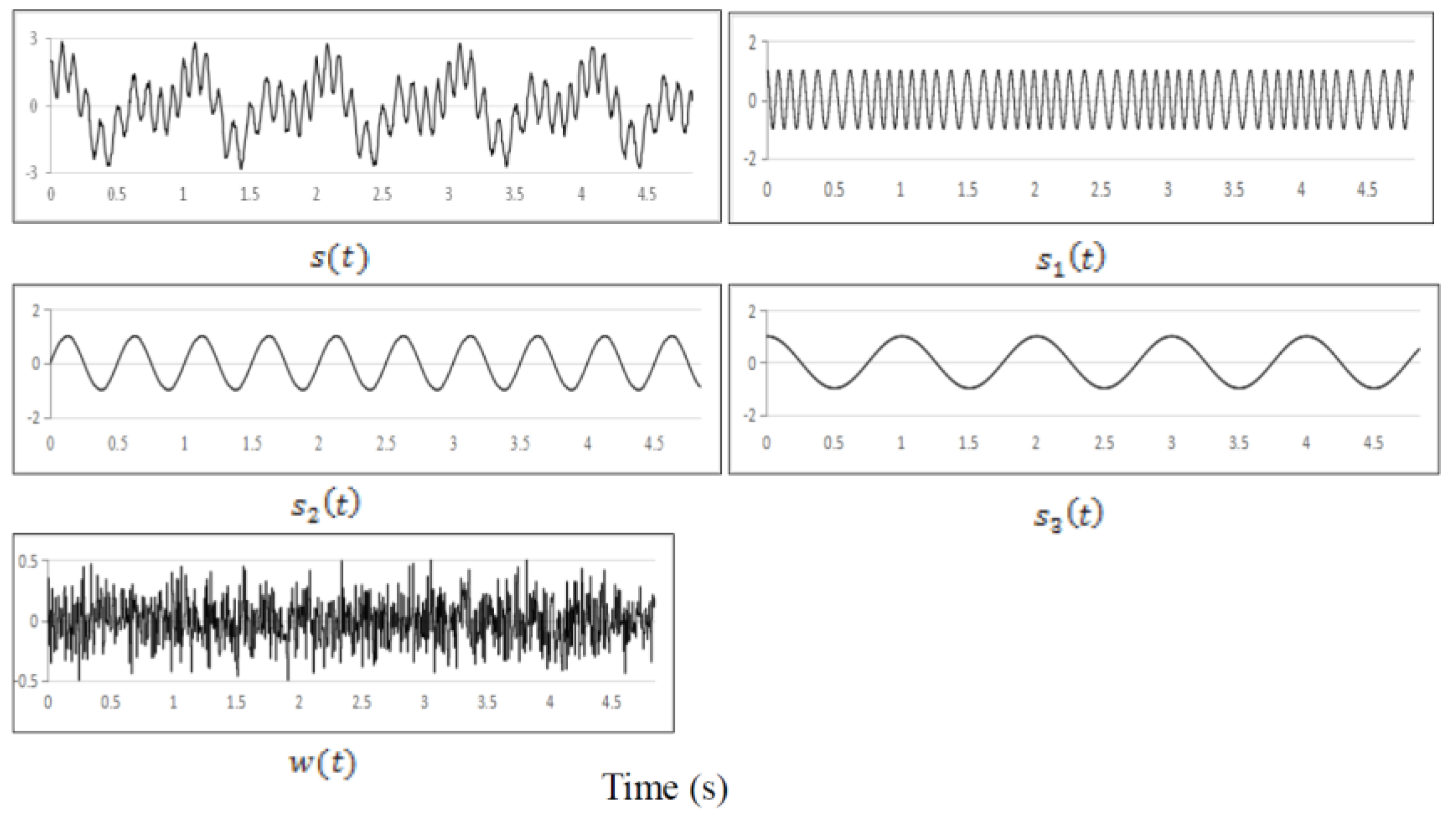
In this study, aiming to demonstrate the validity of the ESMD method compared to the HHT-EMD method [15], a nonlinear and non-stationary signal is simulated by adding white Gaussian noise to three useful sub-signals with an SNR of 20 dB. Where , , , and is white Gaussian noise. The waveforms of the simulation signal and its component signals , , and are shown in Figure 4.
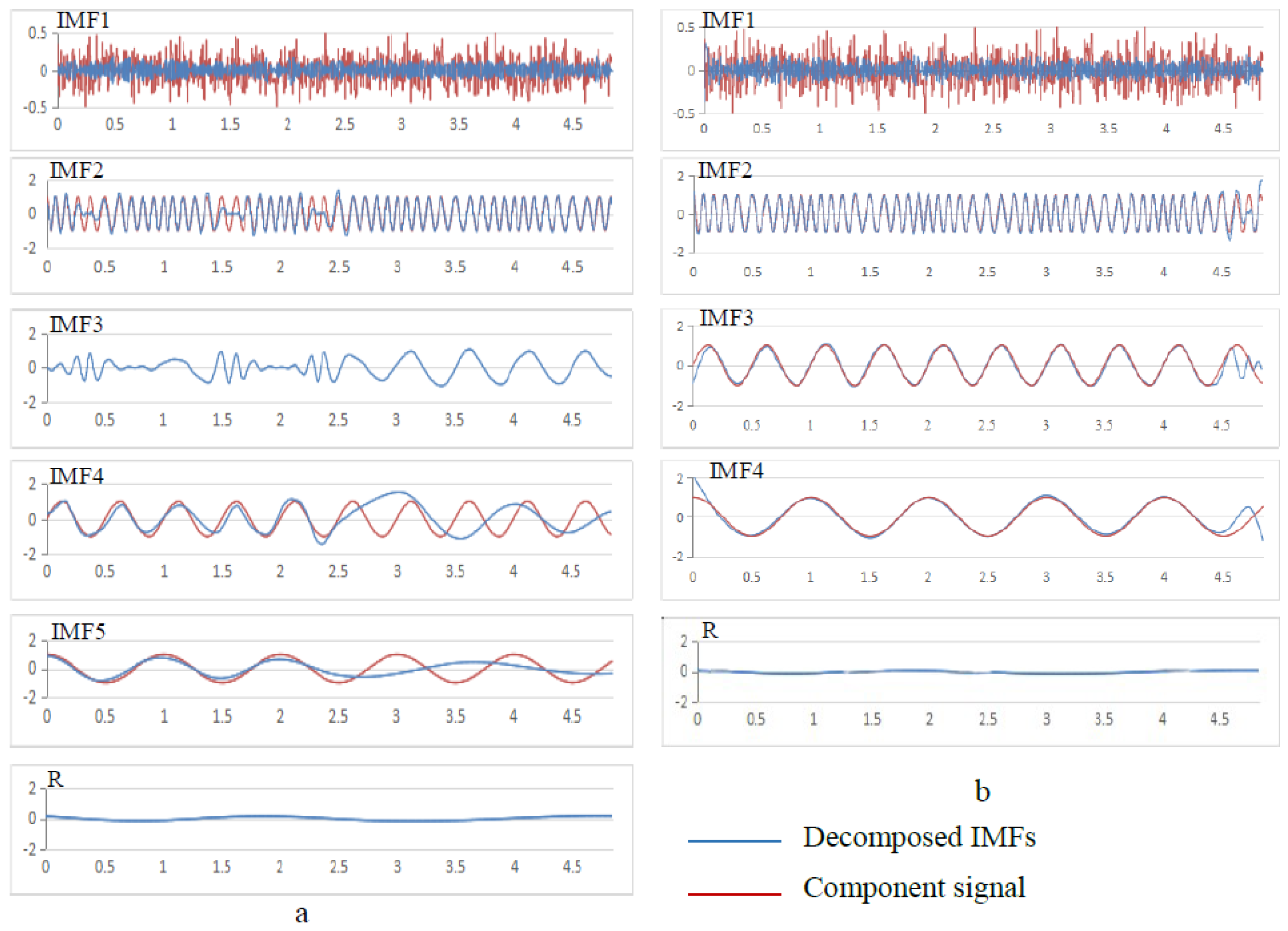
Through the use of the ESMD method and the HHT-EMD method, respectively, the simulation signal is decomposed into a series of IMFs, which are the red curves shown in Figure 5. Moreover, the blue curves of the component signals are exhibited along with their corresponding IMFs. As shown in Figure 5a, through the use of the HHT-EMD method, the simulation signal is decomposed into five IMFs. The decomposed IMF2 is close to even though some local errors exist due to mode mixing problems. However, in the posterior halves of IMF3 and IMF4, they are very different from component signals and on account of some overshoot and undershoot problems. As shown in Figure 5b, through the use of the ESMD method, the simulation signal is decomposed into four IMFs, which are equal to the number of component signals. Furthermore, the mode mixing problems and overshoot and undershoot problems almost disappear, and IMF2 to IMF4 accord with component signals , , and , indicating that the ESMD method performs better than the HHT-EMD method in decomposing a signal into a series of physically meaningful representations.
4.2. Results of Time Series Displacements from Ground-Based Microwave Interferometry
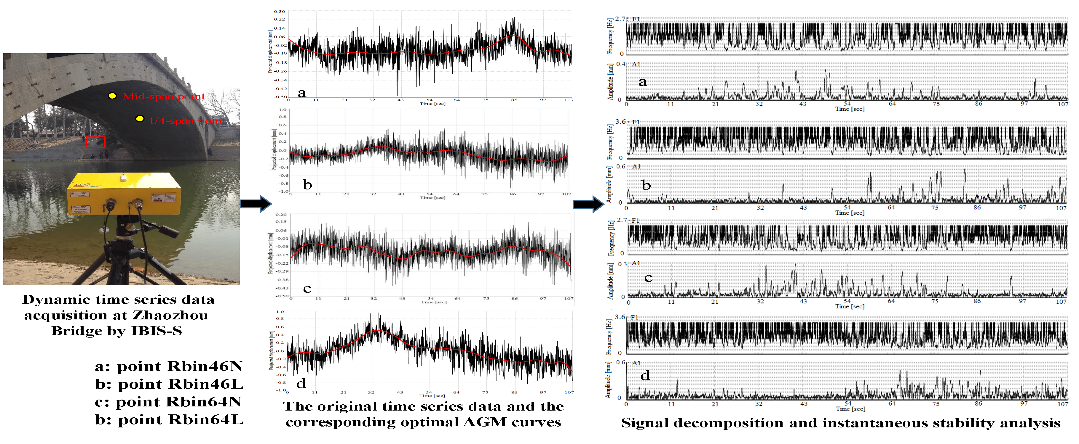
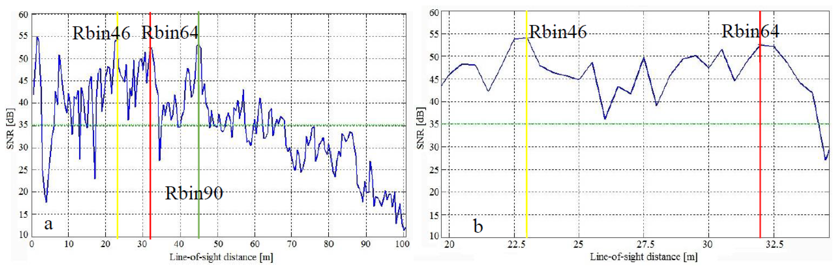
Through using IBIS-S in this study, the whole scene of the lower surface of Zhaozhou Bridge was measured inside the radar beam. Therefore, according to the range resolution of 0.5 m of IBIS-S and the central span of 37.47 m of Zhaozhou Bridge, the dynamic responses of about 30 points can be obtained. However, in the field of civil engineering, the mid-span point and the 1/4-span point are the two key locations used to reflect the dynamic response of a bridge. Therefore, in this study, four kinds of dynamic time series displacements were acquired to perform the instantaneous vibration analysis of Zhaozhou Bridge at the location of the mid-span point and the 1/4-span point, as shown in Figure 2. Two of them were acquired only with environmental excitation factors for the mid-span point with a line-of-sight distance of 23 m to the radar unit (named Rbin46_N) and the 1/4-span point with a line-of-sight distance of 32 m to the radar unit (named Rbin64_N). The other two kinds of dynamic time series displacements were obtained with the transient load of a car for the mid-span point (named Rbin46_L) and the 1/4-span point (named Rbin64_L). In order to ensure the reflected intensity of the electromagnetic wave from the natural surface of Zhaozhou Bridge, the thermal SNR—a ratio between the power of the received signal of a pixel and the thermal noise power of the sensor—was calculated, which can determine the measurement accuracy of the IBIS-S instrument [36]. Generally, when the thermal SNR is better than 30 dB, the standard deviation of measured displacement can reach 0.09 mm for the IBIS-S instrument [37]. Therefore, the empirical thermal SNR of 35 dB was set as the critical value to ensure that the measurement accuracy was better than 0.05 mm for the IBIS-S instrument. As shown in Figure 6, the thermal SNR was 53.8 dB for point Rbin46 and 52.5 dB for point Rbin64, which could ensure that accurate displacements could be obtained by ground-based microwave interferometry. Moreover, another interesting peak occurred at about 45 m (point Rbin90, as shown in Figure 6) along the line-of-sight direction to the radar unit, whose thermal SNR was 53.3 dB. However, as the central span is 37.47 m for Zhaozhou Bridge, point Rbin90 was beyond the scope of the monitored Zhaozhou Bridge. As the area within a red rectangle shown in Figure 2, there is a vertical retaining wall with a smooth surface at the end side of Zhaozhou Bridge in front of the IBIS-S instrument, which can be regarded as a strong backscatter. Furthermore, it has a distance of about 45 m from the vertical retaining wall to the IBIS-S instrument. Therefore, the interesting peak of point Rbin90 may be caused by the vertical retaining wall.
In this study, in order to facilitate the contrast analysis between the time series displacements acquired only with environmental excitation factors and with the transient load of a car, the length of the time series displacements acquired only with environmental excitation factors was shortened to about 107 s, which was the same as the length of the time series displacements acquired with the transient load of a car. For each set of time series displacements, the vertical component of the corresponding projected displacement—a linear displacement perpendicular to the horizontal plane—was calculated as the input time series displacements for further analysis [10]. The curves of the projected displacements of points Rbin46_N and Rbin64_N are shown in Figure 7a,c. As a relative displacement of the acquired projected displacement, the initial reference displacement was defined as 0 mm. The inspection of the projected displacement curves clearly highlights that: (1) the trend of the projected displacement curve of point Rbin46_N (Figure 7a) is similar to that of point Rbin64_N (Figure 7c); and (2) most of the displacement differences are less than 0.3 mm between the adjacent wave peak and wave bottom for the two points, which can be considered as an acceptable displacement difference for Zhaozhou Bridge with the environmental excitation factors.
The curves of the projected displacements of points Rbin46_L and Rbin64_L are shown in Figure 7b,d. The inspection of the projected displacement curves clearly highlights that: (1) compared with the projected displacement curve of points Rbin46_N and Rbin64_N acquired only with the environmental excitation factors, the displacement differences are greatly enlarged for the acquired projected displacements with the transient load of a car, especially for point Rbin64_L with a maximum displacement difference of up to 1 mm between the adjacent wave peak and wave bottom at the time of 35 s (Figure 7d); and (2) compared with the projected displacement curve of point Rbin46_L, the projected displacement curves are more complex and the displacement differences are much bigger than those of point Rbin64_L. These results indicate that the main stress point is located at the 1/4 span point of Zhaozhou Bridge.
4.3. Results of IMF Decomposition and Analysis
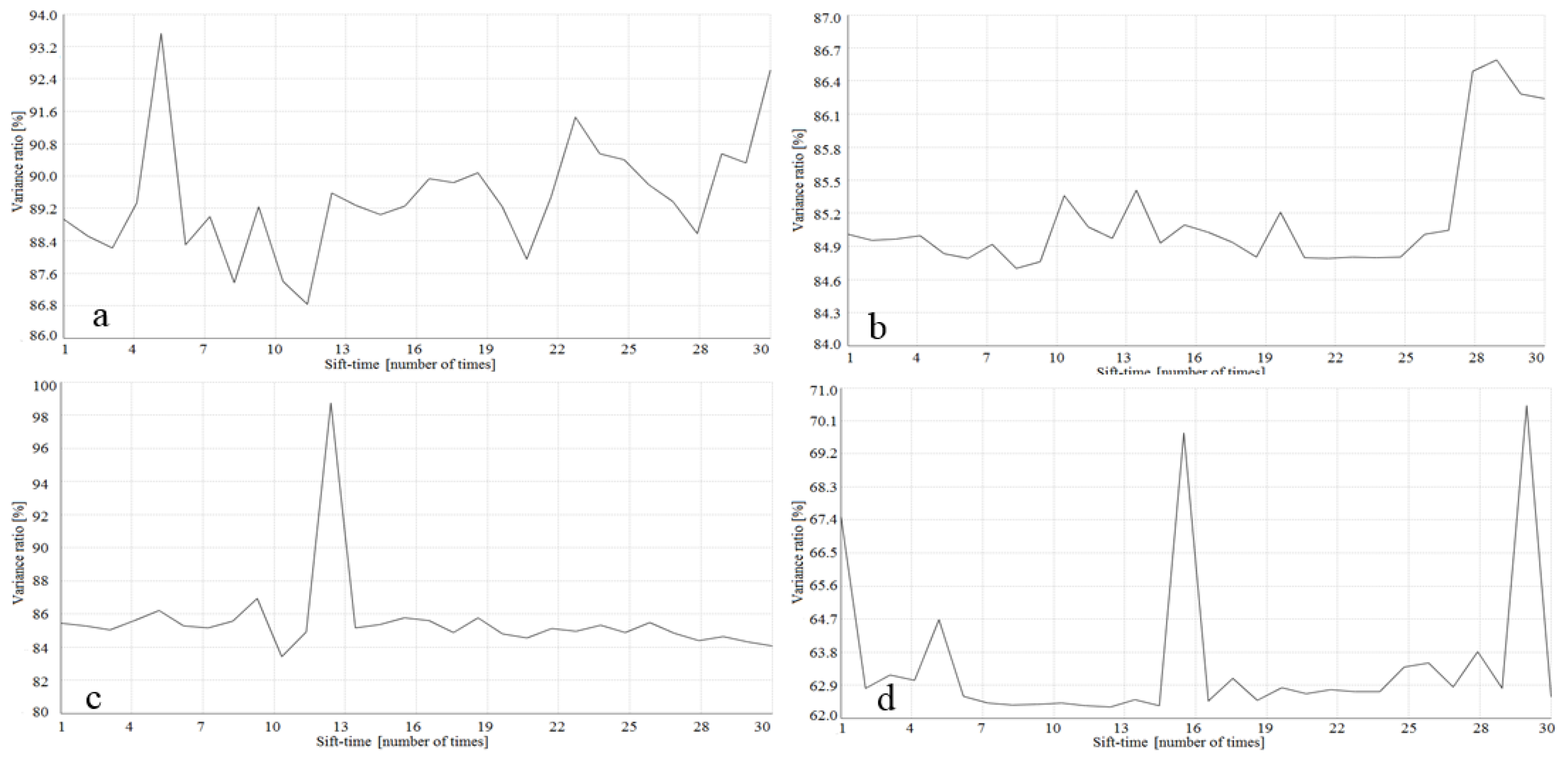
In order to acquire the optimal AGM curves, and to yield a series of IMFs, the optimal variance ratio and the corresponding sifting time needed to be calculated according to (2). In this study, considering the complexity of the time series displacements, the number of extreme points of the last residual was set as 12 (step 6 in Figure 3) and the maximum number of iterations was set as 30 (step 7 in Figure 3). Therefore, the resulting variance ratio figures were acquired as shown in Figure 8. The minimum variance ratio and the corresponding sifting times of the four kinds of time series displacements are shown in Table 2.
According to the acquired minimum variance ratio and the sifting time, a series of IMFs were yielded, together with the optimal AGM curves, for the four kinds of time series displacements. The four optimal AGM curves for the projected displacement curves are shown in Figure 7.
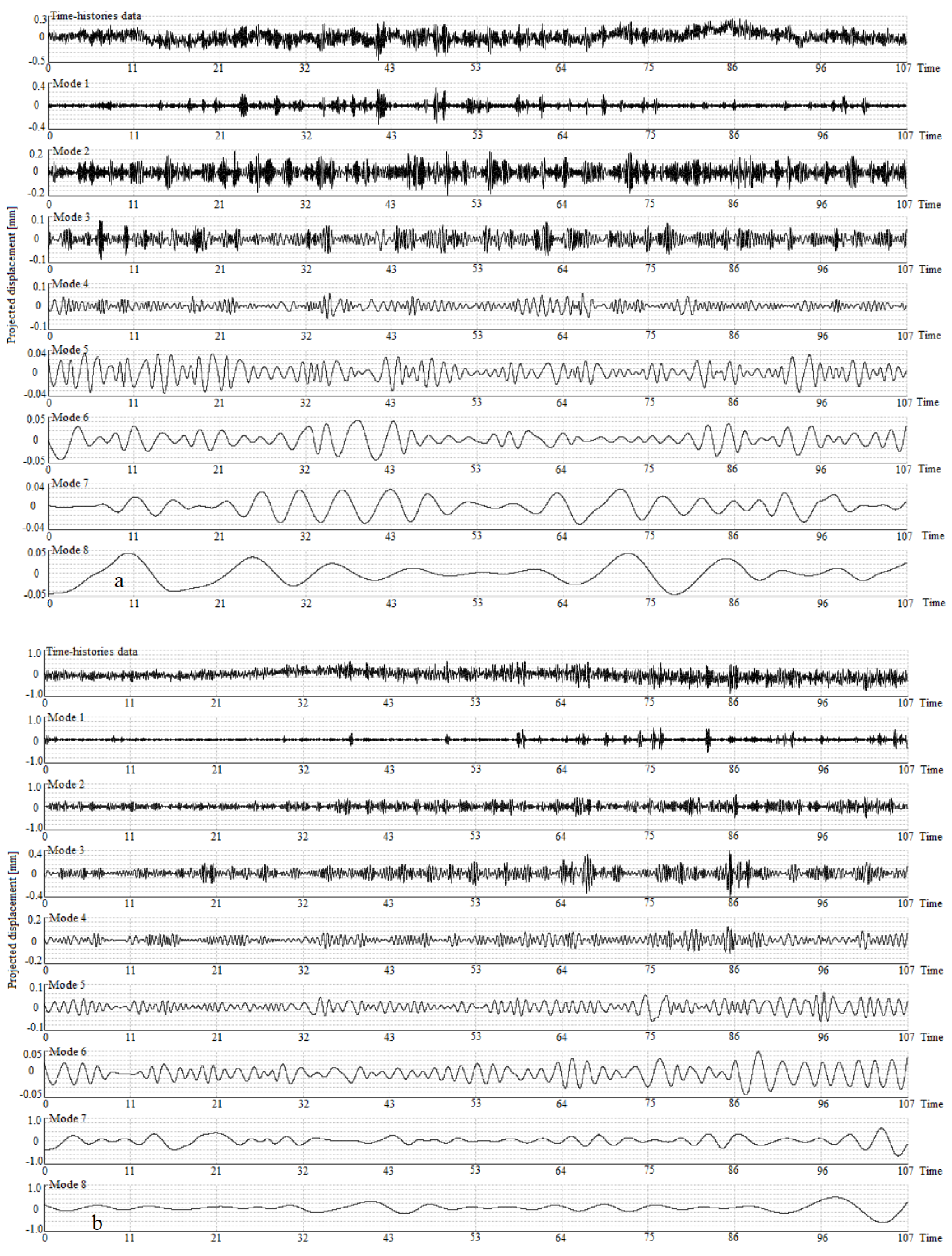
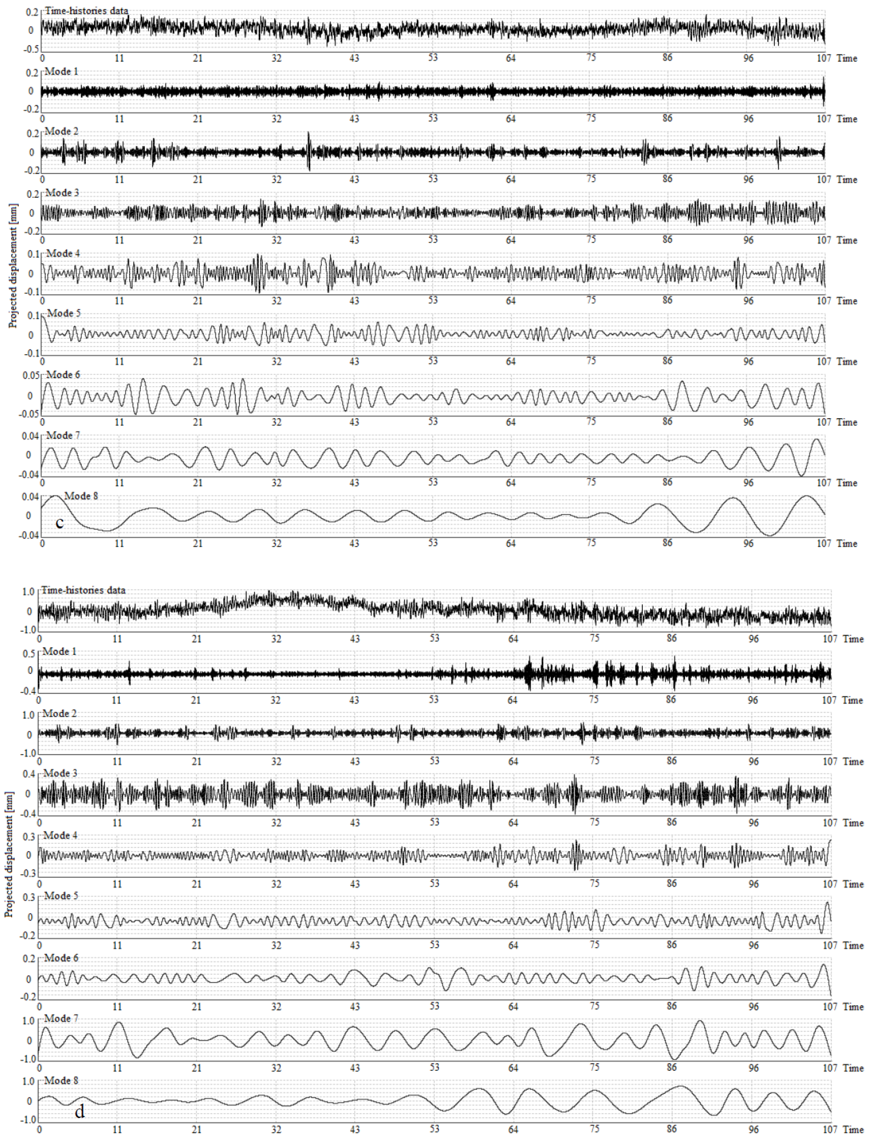
As shown in Figure 9, each set of time series displacements was decomposed into eight IMF components (Mode 1 to Mode 8) via the ESMD method. The inspection of the IMFs in this figure clearly highlights that: (1) For the IMFs of point Rbin46_N (Figure 9a) and point Rbin64_N (Figure 9c), the projected displacement variations gradually decrease from Mode 1 to Mode 8. Unlike the IMFs of point Rbin46_N and point Rbin64_N, the variation of the projected displacements gradually decreases from Mode 1 to Mode 6 for point Rbin46_L (Figure 9b) and point Rbin64_L (Figure 9d), and the projected displacement variation of Mode 7 and Mode 8 is in the interval of −1 mm to 1 mm, which is the same as the corresponding original time series displacements. This reflects the overall vibration trend of Zhaozhou Bridge with the transient load of a car. (2) Many obvious sudden variations appear on the projected displacement curves of Mode 1 and Mode 2 of point Rbin46_N (Figure 9a), but only some small sudden variations occur on the projected displacement curves of Mode 1 and Mode 2 of point Rbin64_N (Figure 9c). This phenomenon indicates that the mid-span point is much more likely to be affected by the environmental excitation factors than the 1/4 span point of Zhaozhou Bridge.
Figure 10 shows the decomposed IMF components of point Rbin64_L obtained via the HHT-EMD method [18]. Compared with the decomposed IMFs of point Rbin64_L obtained via the ESMD method, as shown in Figure 9d, the displacement curves of the main IMFs of Mode 1 to Mode 4 have the same trend, which validates the correctness of the decomposed IMFs obtained via the ESMD method. Nevertheless, using the HHT-EMD method, 12 IMFs are decomposed, which is more than the eight IMFs obtained via the ESMD method, and the displacement curve trends of Mode 5 to Mode 12 are coarse compared with those of Mode 5 to Mode 8 decomposed by the ESMD method.
4.4. Results of Time-Frequency Analysis
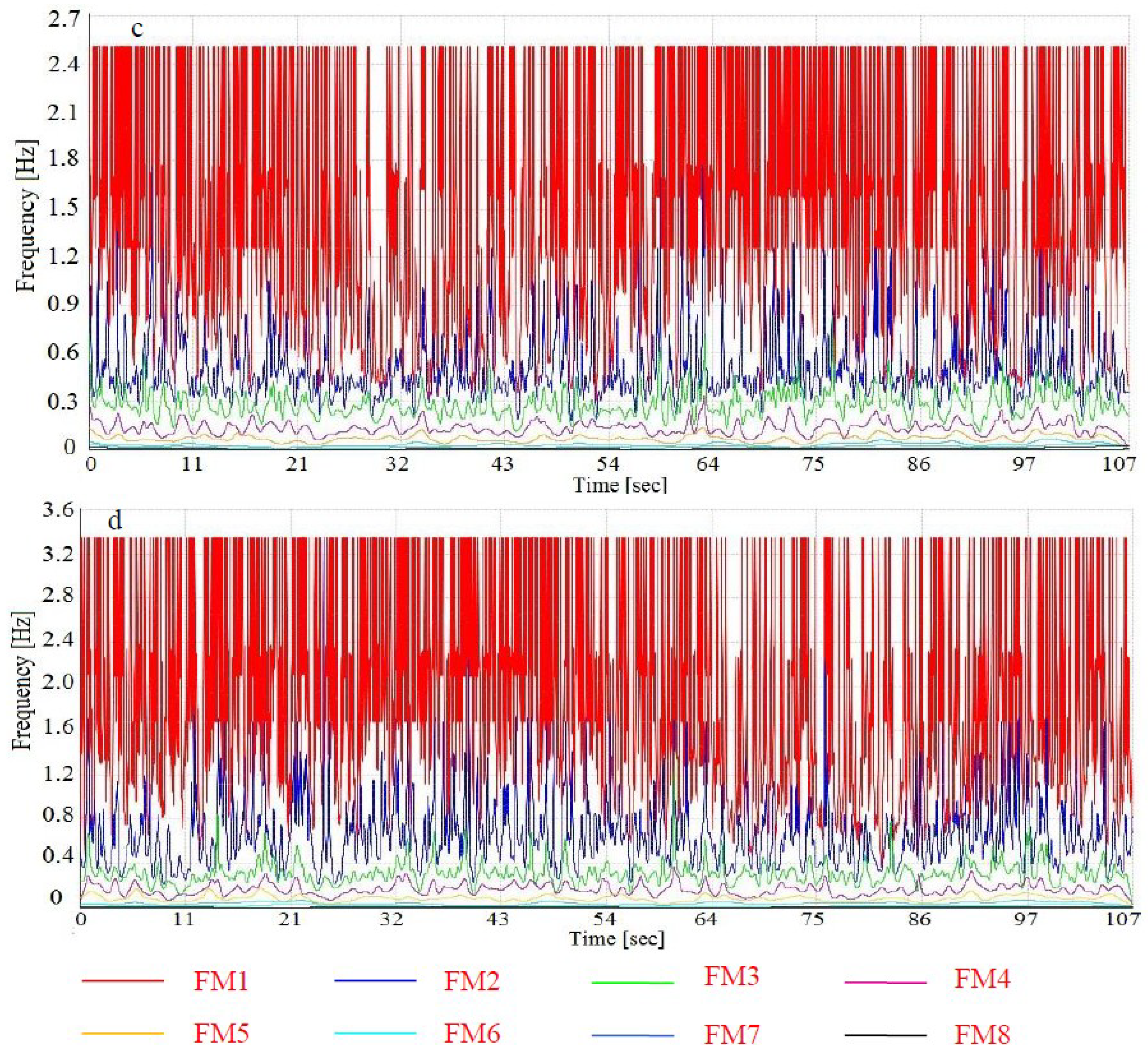
Using the proposed direct interpolation algorithm, the instantaneous frequency and amplitude of each IMF for each set of time series displacements could be calculated. Figure 11 shows the curves of acquired instantaneous frequency of Mode 1 to Mode 8 (FM1 to FM8) with different colors for each set of time series displacements. The instantaneous frequency of each IMF reduces gradually from Mode 1 to Mode 8 for each set of time series displacements. Thereinto, the red curve indicates the instantaneous frequency of Mode 1 for each set of time series displacements. According to the decomposed IMFs, as shown in Figure 9, the main projected displacement variations focus on Mode 1 and Mode 2, and especially Mode 1. Furthermore, compared with the projected displacement curves of Mode 1 for point Rbin46_N and point Rbin64_N, more sudden variations appear on the projected displacement curves of Mode 1 for point Rbin46_L and point Rbin64_L. These results indicate that the projected displacement curve of Mode 1 is the main projected displacement variation related to the bridge, which is the same as HHT [2,21]. Moreover, in order to estimate the efficiency of the instantaneous frequency of Mode 1 from noisy data to evaluate the instantaneous dynamic response of Zhaozhou Bridge, the instantaneous frequencies F1 to F4 with a mean (MN) greater than 0.1 Hz, corresponding to the decomposed Mode 1 to Mode 4 for each set of time series displacement, were selected to make a comparison. The standard deviation (SD) of data must always be understood in the context of the mean of the data, and there is a big difference in the mean of the instantaneous frequencies F1 to F4 for each set of time series displacements, as shown in Table 3. Therefore, in this study, the coefficient of variation (CV) was adopted to evaluate the dispersion of the frequency distribution, which is defined as the ratio of the SD to the MN. As shown in Table 3, the CVs of the instantaneous frequency F1 for each set of time series displacements are much less than those of the corresponding instantaneous frequencies F2 to F4. This further indicates that the projected displacement curve of Mode 1 is the main projected displacement variation related to the bridge. In addition, for the time series displacements with the transient load of a car (points Rbin46_Y and Rbin64_Y), the CVs of instantaneous frequency F1 are somewhat larger than the acquired CVs of instantaneous frequency F1 for the time series displacements with environmental excitation factors (points Rbin46_N and Rbin64_N). The reason for this is that the dispersion of instantaneous frequency distribution can be reduced by the external force of the transient load of a car related to the main projected displacement variation of Zhaozhou Bridge.
Figure 12 shows the instantaneous frequency and amplitude of Mode 1 for each set of time series displacements. The inspection of the instantaneous frequency and amplitude shown in this figure clearly highlights that: (1) For the instantaneous frequency of Mode 1 for each set of time series displacements, there is an apparent saturation effect in the frequency distribution, which is a neat value for the maximum instantaneous frequency, as shown in Figure 11 and Figure 12. The reason for this is that it is a periodic oscillating manner for the structural vibration responses of Zhaozhou Bridge. Most of the resulting adjacent quasi-extreme points and are extreme points which have the same time intervals. Therefore, according to Step 2 of the direct interpolation algorithm, most of the instantaneous frequencies of the discrete points are calculated by , and are also the maximum instantaneous frequencies. Therefore, there is an apparent saturation effect in the frequency distribution of the instantaneous frequency of Mode 1 for each set of time series displacements. These results further indicate that the projected displacement curve of Mode 1 is the main projected displacement variation related to the bridge. (2) Instantaneous frequency is generally a transient structural vibration response which depends on the structural natural frequency, the damping, the stiffness, and the excitation conditions [20]. Therefore, in this study, for the time series displacements acquired only with environmental excitation factors, the maximum instantaneous frequency is about 2.49 Hz for point Rbin46_N (Figure 12a) and point Rbin64_N (Figure 12c). However, when affected by the transient load of a car which is a stronger excitation condition, the maximum instantaneous frequency of Mode 1 of point Rbin46_L (Figure 12b) and point Rbin64_L (Figure 12d) increases to 3.37 Hz. (3) Generally speaking, if some damage has occurred in a structure, this will cause a reduction in the structural natural frequency, which can be reflected by the reduction of the instantaneous frequency of the structures for HHT [33]. In this study, for the direct interpolation algorithm, if some damage had occurred in Zhaozhou Bridge with the transient load of a car, the periodic oscillating manner of the structural vibration response of Zhaozhou Bridge would have been affected. In other words, for the time series displacements acquired after the transient load of a car, the number of adjacent quasi-extreme points being extreme points would have been greatly reduced. Therefore, according to Step 2 of the direct interpolation algorithm, the number of instantaneous frequencies being the maximum instantaneous frequency should also be greatly reduced. However, as shown in Figure 12b,d, there is an approximately uniform distribution for the maximum instantaneous frequency of Mode 1. This indicates that Zhaozhou Bridge was in an instantaneous stable state when the car passed over Zhaozhou Bridge. (4) The maximum instantaneous frequency of Mode 1 is obtained in conjunction with most of the lower amplitudes. However, there are some decreased instantaneous frequencies of Mode 1 corresponding to the higher amplitudes. The reason for this is that the higher amplitudes are caused by the environmental excitation factors or the transient load of a car, which can affect the periodic oscillating manner of Zhaozhou Bridge. Furthermore, the maximum amplitude (A1) of Mode 1 for point Rbin46_N is about 0.34 mm, which is a little bigger than the 0.29 mm for point Rbin64_N. However, the maximum amplitude (A1) of Mode 1 for point Rbin46_L increases to 0.55 mm, which is also bigger than the 0.46 mm for point Rbin64_L. These results further indicate that the main stress point is located at the 1/4 span point rather than the mid-span point.
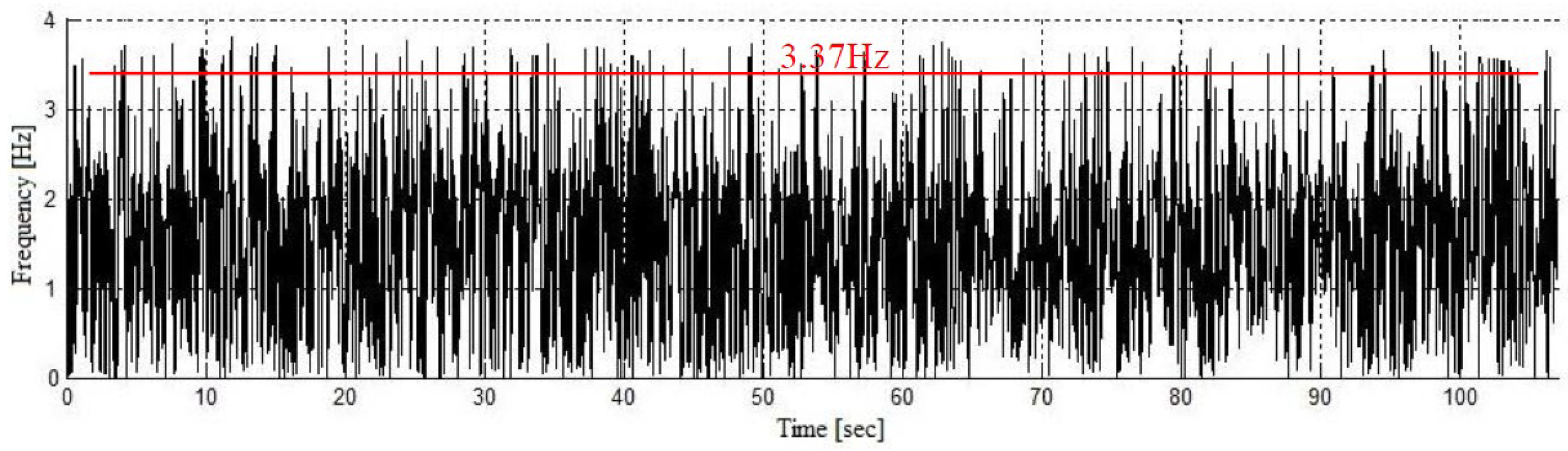
Figure 13 shows the instantaneous frequency of Mode 1 of point Rbin64_L obtained by HHT [18]. Compared with the instantaneous frequency of Mode 1 of point Rbin64_L obtained by the ESMD method, as shown in Figure 12c, most of the peaks of instantaneous frequency are lower than 3.37 Hz (red line in Figure 13), which is the constant maximum instantaneous frequency of Mode 1 of point Rbin64_L obtained by the ESMD method, as shown in Figure 12d. Furthermore, there are no sudden changes in the curve of the obtained instantaneous frequency of Mode 1 of point Rbin64_L obtained by HHT, which also indicates that Zhaozhou Bridge was in a steady state when the car passed over the bridge. However, there are some larger differences among the peaks of the instantaneous frequency for Mode 1 of point Rbin64_L obtained by HHT. In other words, it is difficult to identify the minor damage if some smaller sudden changes exist in the curve of the instantaneous frequency obtained by HHT. However, for the ESMD method, because the acquired maximum instantaneous frequency is constant for the undamaged parts of the structure, it is easy to detect the damage, which is an advantage of the ESMD method.
5. Discussion
This paper explored a non-contact approach for the joint use of ground-based microwave interferometry and the ESMD method, with the purpose of the instantaneous vibration analysis of ancient bridges. Ground-based microwave interferometry was adopted to obtain the accurate time series displacements of the monitored ancient bridge, and the ESMD method was adopted to perform the instantaneous vibration analysis of the monitored ancient bridge by the decomposed IMFs and the corresponding instantaneous frequencies. Based on the results of the aforementioned experiment for Zhaozhou Bridge, there are three issues that need to be discussed, as follows.
- (1)
- By adopting IBIS-S to obtain the time series displacements of Zhanzhou Bridge, ground-based microwave interferometry has been validated as an effective non-contact technique to monitor ancient bridges. Without passive radar reflectors installed on the surface of ancient bridges, the thermal SNR values of all of the monitoring points were larger than 35 dB, which could ensure that accurate displacements were obtained. Therefore, for the purpose of avoiding any damages on Zhaozhou Bridge, the traditional transducers were not attached on the bridge to evaluate the accuracy of ground-based microwave interferometry. However, as ground-based microwave interferometry makes use of the propagation of electromagnetic waves for displacement measurement, the measurements performed are inevitably influenced by the atmospheric refractive index, which is caused by temperature, humidity, air pressure, and other meteorological factors [38]. Different meteorological conditions have different atmospheric refractive index values, which can cause some loss of measurement accuracy. Therefore, if there is a need for the periodic monitoring of bridges in different measuring times using ground-based microwave interferometry, it is necessary to improve the measurement accuracy of the dynamic deflection of bridges by the use of atmospheric parameters correction, such as the Permanent Scatterers technique [38,39,40] and model-based approach [10,41]. This can improve the contrast of different period data. However, in this study, the acquisition time of all data only lasts about 30 min, and has almost the same influence of meteorological factors for displacement measurement. Moreover, the purpose of this paper is to perform the instantaneous vibration analysis of ancient bridges. Hence, it is not necessary to compensate for the propagation losses in this study, which will not affect the reliability of the instantaneous vibration analysis of ancient bridges.
- (2)
- Generally, any one complicated signal can be regarded as being composed of multiple simple signals which represent different physical meanings [32]. In this study, through the use of the ESMD method, the acquired time series displacements was decomposed into eight IMFs together with an optimal AGM curve, which are more accurate compared with the decomposed 12 IMFs by the HHT-EMD method. Furthermore, by analyzing the decomposed IMFs, the overall vibration trend and sudden variations of the projected displacement can be obtained to analyze the structural characteristics of ancient bridges. However, it is difficult to obtain the physical meaning of each IMF, which needs to be further studied. Moreover, the thrust of wind, ground-motion, complicated traffic, etc., will inevitably generate a noise signal that reduces the accuracy of the measured dynamic displacement of the bridge. In addition, the monitored bridge itself also has a periodic vibration, of which the vibration frequency is different from the transient vibration by the instant loading of a car. Therefore, the obtained dynamic displacement of the bridge, caused by the instant loading of a car, should become bigger or smaller. To the authors’ best knowledge, there is not a theoretical model or a gold standard method to determine the expected dynamic displacement in the bridge caused by the instant loading of a car. Further study of the denoising algorithm is also needed to improve the accuracy of the expected dynamic displacement caused by the instant loading. Nevertheless, the above factors influence the expected dynamic displacement caused by the instant loading a little, which will not affect the instantaneous vibration analysis in this study.
- (3)
- Instantaneous frequency is a transient structural vibration response, which not only depends on the structural natural frequency, but is also influenced by the damping, the stiffness, and the excitation conditions [20,42]. In this study, the obtained maximum instantaneous frequency is 2.49 Hz for Mode 1 only with environmental excitation factors. However, due to the stronger excitation condition of a transient load of a car, the obtained maximum instantaneous frequency increases to 3.37 Hz for Mode 1. Therefore, by using the ESMD method, it can accurately identify the variations of instantaneous frequency by a neat value for the maximum instantaneous frequency. Furthermore, it is generally known that the structural natural frequency will be reduced if some damage occurs in a structure, which can be reflected by the sudden reduction of the instantaneous frequency of the monitored structure [43,44]. In this study, according to the direct interpolation algorithm, if some damage had occurred in Zhaozhou Bridge with the transient load of a car, the instantaneous frequencies of Mode 1 should be decreased steadily. Therefore, although the maximum instantaneous frequency changed from 2.49 Hz to 3.37 Hz for Mode 1, there was no sudden steady decrease in the curve of instantaneous frequency, which indicates that it was in an instantaneous stable state when the car passed over Zhaozhou Bridge. However, Zhaozhou Bridge has been operational for 1400 years now, so if we want to detect the significant changes for the purpose of a global stability analysis, a large period of several months may be required.
6. Conclusions
In order to evaluate the instantaneous dynamic response of ancient bridges, this paper proposed an integrated method consisting of ground-based microwave interferometry and the ESMD method and applied it to the well-known Zhaozhou Bridge. Ground-based microwave interferometry was adopted to acquire the dynamic time series displacements with environmental excitation factors and a transient load with a car, respectively. The ESMD method was used to decompose the time series displacements into a series of IMFs and the corresponding instantaneous frequencies, which were then used to perform the instantaneous vibration analysis of Zhaozhou Bridge. More specifically, the results presented in the paper clearly highlight that:
- (1)
- In this study, aiming to avoid damage to the great historical heritage for Zhaozhou Bridge, the IBIS-S instrument was only located on one side of Zhaozhou Bridge without corner reflectors attached on the lower surface of Zhaozhou Bridge. The quick and easy installation of the IBIS-S instrument can greatly improve the efficiency of data collection. Moreover, the resulting thermal SNR of all of monitoring points on the lower surface of the bridge were larger than 35 dB, which could ensure that accurate displacements were obtained. Therefore, these results verify the feasibility and accuracy of the dynamic monitoring of Zhaozhou Bridge by the sensing method of ground-based microwave interferometry in the paper, which further indicates that ground-based microwave interferometry is a viable alternative technique to acquire dynamic time series displacements for the instantaneous vibration analysis of ancient bridges. Meanwhile, it can also reduce the inherent risk involved with the placement of the traditional contact transducers.
- (2)
- The ESMD method was performed to yield a series of IMFs together with an optimal AGM curve through the use of a mode symmetric about the maxima and minima points. The decomposed IMFs can reflect the overall tendency of the projected displacement according to the magnitude of the frequency. Furthermore, they can also reflect the instantaneous dynamic response of the different monitored points.
- (3)
- The instantaneous frequencies were obtained using the direct interpolation algorithm, which can reconcile the conflict between the period and the frequency, compared with the traditional time-frequency analysis methods. The instantaneous frequencies of the decomposed IMFs of each set of time series displacements showed that Zhaozhou Bridge was in a steady state when the car passed over the bridge.
- (4)
- Compared with the use of HHT for obtaining decomposed IMFs and instantaneous frequencies, the results showed that the proposed method is a new and powerful alternative technique for the instantaneous vibration analysis of ancient bridges.
Author Contributions
X.L. and X.T. conducted the algorithm design. X.L. wrote the paper. X.T. revised the paper. Z.L. and M.H. contributed to acquiring time series displacements of Z.B. W.Y. contributed to studying the ESMD method in order to analyze the instantaneous dynamic response of Z.B. All authors have contributed significantly and have participated sufficiently to take responsibility for this research.
Funding
This work has been funded by the National Natural Science Foundation of China (grant 41501494, 41401528), the Importation and Development of High-Caliber Talents Project of Beijing Municipal Institutions (grant CIT&TCD201704053), and the Talent Program of Beijing University of Civil Engineering and Architecture.
Conflicts of Interest
The authors declare no conflict of interest.
References
- Liu, X.L.; Tong, X.H.; Yin, X.J.; Gu, X.L.; Ye, Z. Videogrammetric technique for three-dimensional structural progressive collapse measurement. Measurement 2015, 63, 87–89. [Google Scholar] [CrossRef]
- Roveri, N.; Carcaterra, A. Damage detection in structures under traveling loads by Hilbert–Huang transform. Mech. Syst. Signal Process. 2012, 28, 128–144. [Google Scholar] [CrossRef]
- Lee, J.W.; Kim, J.D.; Yun, C.B.; Yi, J.H.; Shim, J.M. Health-monitoring method for bridges under ordinary traffic loading. J. Sound Vib. 2002, 257, 247–264. [Google Scholar] [CrossRef]
- Heieh, K.M.; Halling, H.W.; Barr, P.J. Overview of vibrational structural health monitoring with representative case studies. J. Bridge Eng. 2006, 11, 707–715. [Google Scholar]
- Xu, Y.L.; Chen, B.; Ng, C.L.; Wong, K.Y.; Chan, W.Y. Monitoring temperature effect on a long suspension bridge. Struct. Control Health Monit. 2010, 17, 632–653. [Google Scholar] [CrossRef]
- Gentile, C.; Bernardini, G. An interferometric radar for non-contact measurement of deflections on civil engineering structures: Laboratory and full-scale tests. Struct. Infrastruct. Eng. 2010, 6, 521–534. [Google Scholar] [CrossRef]
- Pieraccini, M.; Fratini, M.; Parrini, F.; Atzeni, C. Dynamic monitoring of bridges using a high-speed coherent radar. IEEE Trans. Geosci. Remote Sens. 2006, 44, 3284–3288. [Google Scholar] [CrossRef]
- Gentile, C. Application of microwave remote sensing to dynamic testing of stay-cables. Remote Sens. 2009, 2, 36–51. [Google Scholar] [CrossRef]
- Stabile, T.A.; Perrone, A.; Gallipoli, M.R.; Ditommaso, R.; Ponzo, F.C. Dynamic survey of the Musmeci bridge by joint application of ground-based microwave radar interferometry and ambient noise standard spectral ratio techniques. IEEE Geosci. Remote Sens. Lett. 2013, 10, 870–874. [Google Scholar] [CrossRef]
- Liu, X.L.; Tong, X.H.; Ding, K.L.; Zhao, X.A.; Zhu, L.; Zhang, X.D. Measurement of Long-Term Periodic and Dynamic Deflection of the Long-Span Railway Bridge Using Microwave Interferometry. IEEE J. Sel. Top. Appl. Earth Obs. Remote Sens. 2015, 8, 4531–4538. [Google Scholar] [CrossRef]
- Negulescu, C.; Luzi, G.; Crosetto, M.; Raucoules, D.; Roullé, A.; Monfort, D.; Pujades, L.; Colas, B.; Dewez, T. Comparison of seismometer and radar measurements for the modal identification of civil engineering structures. Eng. Struct. 2013, 51, 10–22. [Google Scholar] [CrossRef]
- Pieraccini, M.; Fratini, M.; Parrini, F.; Atzeni, C.; Partoli, G. Interferometric radar vs. accelerometer for dynamic monitoring of large structures: An experimental comparison. NDT & E Int. 2008, 41, 258–264. [Google Scholar]
- Gökdağ, H.; Kopmaz, O. A new damage detection approach for beam-type structures based on the combination of continuous and discrete wavelet transforms. J. Sound Vib. 2009, 324, 1158–1180. [Google Scholar] [CrossRef]
- Khorram, A.; Bakhtiari-Nejad, F.; Rezaeian, M. Comparison studies between two wavelet based crack detection methods of a beam subjected to a moving load. Int. J. Eng. Sci. 2012, 51, 204–215. [Google Scholar] [CrossRef]
- Huang, N.E.; Shen, Z.; Long, S.R.; Wu, M.C.; Shih, H.H.; Zheng, Q.; Yen, N.C.; Tung, C.C.; Liu, M.H. The Empirical Mode Decomposition and the Hilbert Spectrum for Nonlinear and Nonstationary Time Series Analysis. Proc. R. Soc. Lond. 1998, A454, 903–995. [Google Scholar] [CrossRef]
- Wang, J.L.; Li, Z.J. Extreme-Point Symmetric Mode Decomposition Method for Data Analysis. Adv. Adapt. Data Anal. 2013, 5, 1350015. [Google Scholar] [CrossRef]
- Li, H.; Wang, C.; Zhao, D. An improved EMD and its applications to find the basis functions of EMI signals. Math. Probl. Eng. 2015, 150127. [Google Scholar] [CrossRef]
- Huang, N.E.; Wu, Z. A review on Hilbert-Huang transform: Method and its applications to geophysical studies. Rev. Geophys. 2008, 46. [Google Scholar] [CrossRef]
- Quek, S.T.; Tua, P.S.; Wang, Q. Detecting anomalies in beams and plate based on the Hilbert-Huang transform of real signals. Smart Mater. Struct. 2003, 12, 447–460. [Google Scholar] [CrossRef]
- Chen, H.G.; Yan, Y.J.; Jiang, J.S. Vibration-based damage detection in composite wingbox structures by HHT. Mech. Syst. Signal Process. 2007, 21, 307–321. [Google Scholar] [CrossRef]
- Kunwar, A.; Jha, R.; Whelan, M.; Janoyan, K. Damage detection in an experimental bridge model using Hilbert–Huang transform of transient vibrations. Struct. Control Health 2013, 20, 201–215. [Google Scholar] [CrossRef]
- Yang, W.A.; Zhou, W.; Liao, W.; Guo, Y. Identification and quantification of concurrent control chart patterns using extreme-point symmetric mode decomposition and extreme learning machines. Neurocomputing 2015, 147, 260–270. [Google Scholar] [CrossRef]
- Liu, X.L.; Tang, Y.; Lu, Z.; Huang, H.; Tong, X.H.; Ma, J. ESMD-based stability analysis in the progressive collapse of a building model: A case study of a reinforced concrete frame-shear wall model. Measurement 2018, 120, 34–42. [Google Scholar] [CrossRef]
- Song, S.; Ding, M.; Li, H.; Song, X.; Fan, W.; Zhang, X.; Xu, H. Frequency specificity of fMRI in mesial temporal lobe epilepsy. PLoS ONE 2016, 11, e0157342. [Google Scholar] [CrossRef] [PubMed]
- Qian, L.X. New insight into an ancient stone arch bridge—The Zhao-Zhou Bridge of 1400 years old. Int. J. Mech. Sci. 1987, 29, 831–843. [Google Scholar] [CrossRef]
- Au, F.T.K.; Wang, J.J.; Liu, G.D. Construction control of reinforced concrete arch bridges. J. Bridge Eng. 2003, 8, 39–45. [Google Scholar] [CrossRef]
- Audenaert, A.; Peremans, H.; Reniers, G. An analytical model to determine the ultimate load on masonry arch bridges. J. Eng. Math. 2007, 59, 323–336. [Google Scholar] [CrossRef]
- Gentile, C. Deflection measurement on vibrating stay cables by non-contact microwave interferometer. NDT E Int. 2010, 43, 231–240. [Google Scholar] [CrossRef]
- Beben, D. Application of the interferometric radar for dynamic tests of corrugated steel plate (CSP) culvert. NDT E Int. 2011, 44, 405–412. [Google Scholar] [CrossRef]
- Crosetto, M.; Monserrat, O.; Luzi, G.; Cuevas-Gonzalez, M.; Devanthery, N. A noninterferometric procedure for deformation measurement using GB-SAR imagery. IEEE Geosci. Remote Sens. Lett. 2014, 11, 34–38. [Google Scholar] [CrossRef]
- Montuori, A.; Luzi, G.; Bignami, C.; Gaudiosi, I.; Stramondo, S.; Crosetto, M.; Buongiorno, M.F. The Interferometric Use of Radar Sensors for the Urban Monitoring of Structural Vibrations and Surface Displacements. IEEE J. Sel. Top. Appl. Earth Obs. Remote Sens. 2016, 9, 3761–3776. [Google Scholar] [CrossRef]
- Huang, N.E.; Wu, Z.; Long, S.R.; Arnold, K.C.; Chen, X.; Blank, K. On instantaneous frequency. Adv. Adapt. Data Anal. 2009, 1, 177–229. [Google Scholar] [CrossRef]
- Zhang, R.R.; King, R.; Olson, L.; Xu, Y.L. Dynamic response of the Trinity River Relief Bridge to controlled pile damage: Modeling and experimental data analysis comparing Fourier and Hilbert–Huang techniques. J. Sound Vib. 2005, 285, 1049–1070. [Google Scholar] [CrossRef]
- Gonzalez, I.; Karoumi, R. Analysis of the annual variations in the dynamic behavior of a ballasted railway bridge using Hilbert transform. Eng. Struct. 2014, 60, 126–132. [Google Scholar] [CrossRef]
- Carbajo, E.S.; Carbajo, R.S.; Mc Goldrick, C.; Basu, B. ASDAH: An automated structural change detection algorithm based on the Hilbert–Huang transform. Mech. Syst. Signal Process. 2014, 47, 78–93. [Google Scholar] [CrossRef]
- Liu, X.L.; Zhao, X.A.; Ding, K.L.; Zhu, L.; Ma, J.; Dong, Y.Q.; Tong, X.H. Application of ground-based synthetic aperture radar technique for emergency monitoring of deep foundation excavation. J. Appl. Remote Sens. 2015, 9, 096021. [Google Scholar] [CrossRef]
- Rödelsperger, S. Real-Time Processing of Ground Based Synthetic apeRture Radar (GB-SAR) Measurement; Fachbereich Bauingenieurwesen und Geodäsie, Technische Universität Darmstadt: Darmstadt, Germany, 2011. [Google Scholar]
- Noferini, L.; Pieraccini, M.; Mecatti, D.; Luzi, G.; Atzeni, C.; Tamburini, A.; Broccolato, M. Permanent scatterers analysis for atmospheric correction in ground-based SAR interferometry. IEEE Trans. Geosci. Remote Sens. 2005, 43, 1459–1471. [Google Scholar] [CrossRef]
- Pipia, L.; Fábregas, X.; Aguasca, A.; Lopez-Martinez, C. Atmospheric artifact compensation in ground-based DInSAR applications. IEEE Geosci. Remote Sens. Lett. 2008, 5, 88–92. [Google Scholar] [CrossRef]
- Leva, D.; Nico, G.; Tarchi, D.; Fortuny-Guasch, J.; Sieber, A.J. Temporal analysis of a landslide by means of a ground-based SAR interferometer. IEEE Trans. Geosci. Remote Sens. 2003, 41, 745–752. [Google Scholar] [CrossRef]
- Iannini, L.; Guarnieri, A.M. Atmospheric Phase Screen in Ground-Based Radar: Statistics and Compensation. IEEE Geosci. Remote Sens. Lett. 2011, 8, 537–541. [Google Scholar] [CrossRef]
- Amezquita-Sanchez, J.P.; Adeli, H. Signal processing techniques for vibration-based health monitoring of smart structures. Arch. Comput. Method Eng. 2016, 23, 1–15. [Google Scholar] [CrossRef]
- Wang, Z.C.; Xin, Y.; Ren, W.X. Nonlinear structural joint model updating based on instantaneous characteristics of dynamic responses. Mech. Syst. Signal Process. 2016, 76, 476–496. [Google Scholar] [CrossRef]
- Salawu, O.S. Detection of structural damage through changes in frequency: A review. Eng. Struct. 1997, 19, 718–723. [Google Scholar] [CrossRef]
Figure 1.
Sketch of Zhaozhou Bridge.
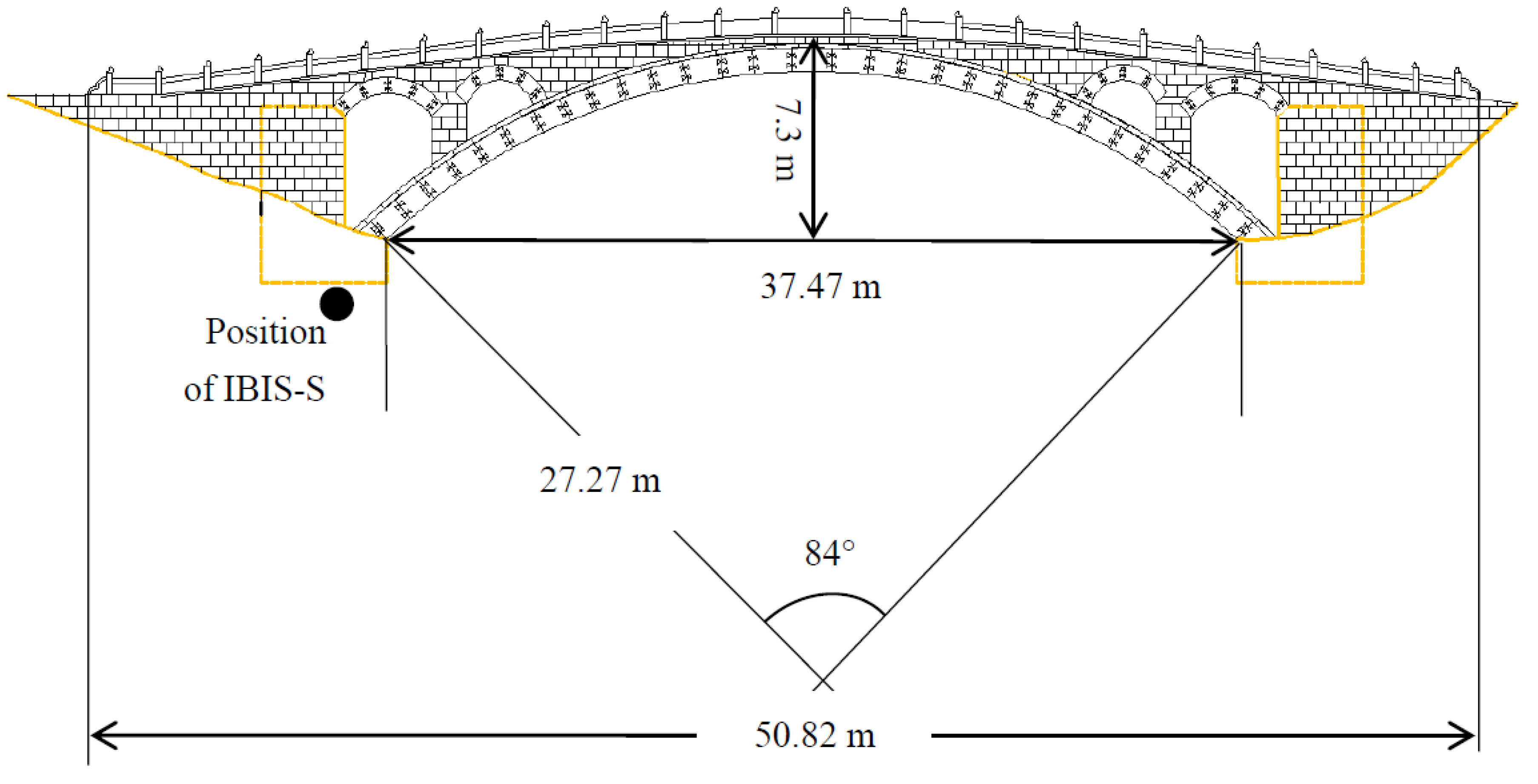
Figure 2.
View of the IBIS-S instrument for dynamic time series displacement acquisition at Zhaozhou Bridge.
Figure 2.
View of the IBIS-S instrument for dynamic time series displacement acquisition at Zhaozhou Bridge.

Figure 3.
The whole decomposition process of the ESMD method to yield a series of IMFs together with an optimal AGM curve.
Figure 3.
The whole decomposition process of the ESMD method to yield a series of IMFs together with an optimal AGM curve.

Figure 4.
The simulation signal and its component signals , , , and .

Figure 5.
IMFs of decomposed by the HHT-EMD method and the ESMD method. (a) IMFs of decomposed by the HHT-EMD method and the exhibited component signals along with their corresponding IMFs; and (b) IMFs of decomposed by the ESMD method and the exhibited component signals along with their corresponding IMFs.

Figure 6.
Curves of the thermal SNR of the received signals. (a) Curve of the thermal SNR of the entire monitoring range; (b) Enlarged curve of the thermal SNR of points Rbin46 and Rbin64.
Figure 6.
Curves of the thermal SNR of the received signals. (a) Curve of the thermal SNR of the entire monitoring range; (b) Enlarged curve of the thermal SNR of points Rbin46 and Rbin64.

Figure 7.
The original time series displacements and the corresponding optimal AGM curves. (a) The original time series displacements and the optimal AGM curve of point Rbin46_N; (b) The original time series displacements and the optimal AGM curve of point Rbin46_L; (c) The original time series displacements and the optimal AGM curve of point Rbin64_N; (d) The original time series displacements and the optimal AGM curve of point Rbin64_L.
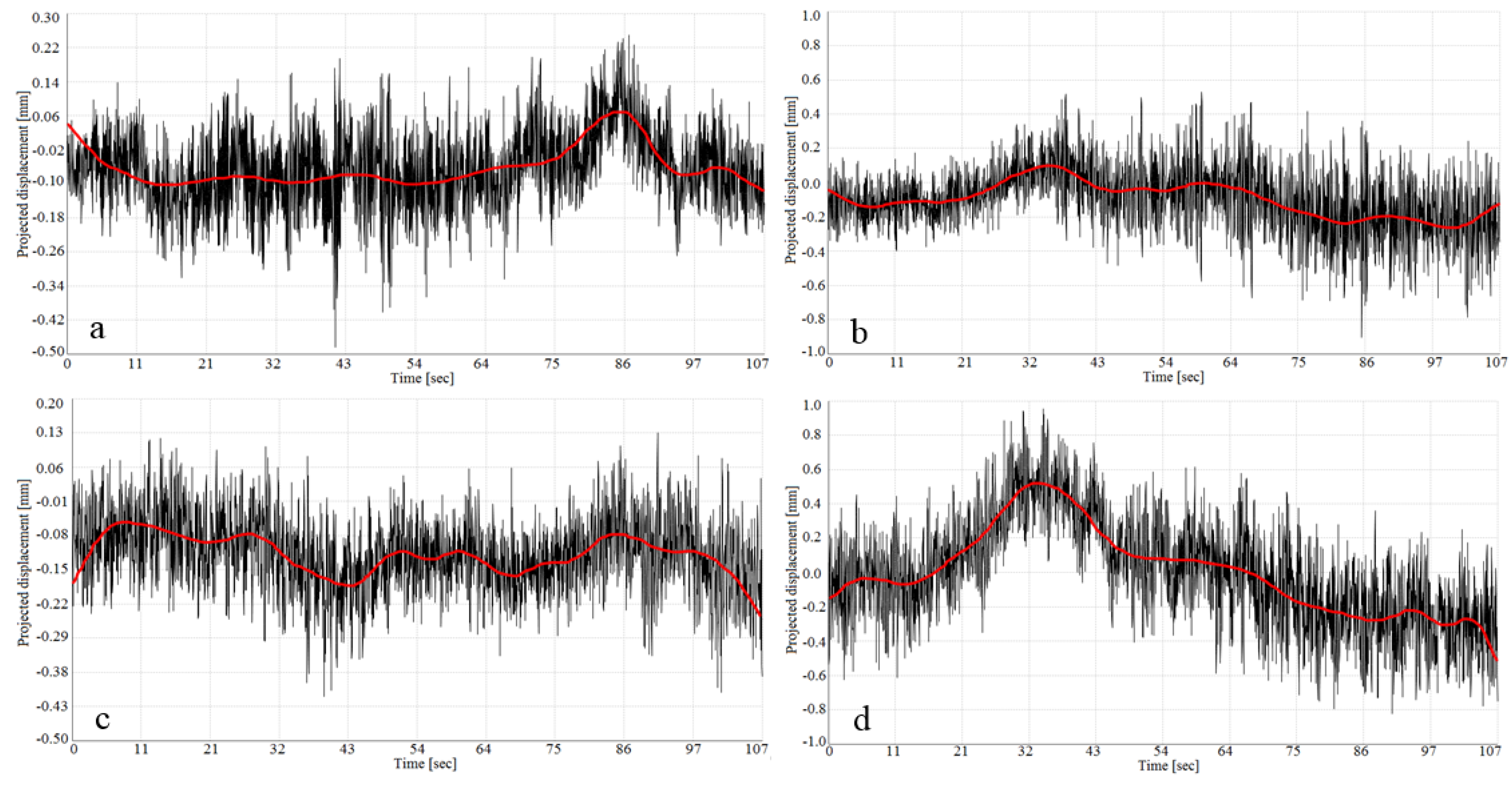
Figure 8.
Variance ratio of the original time series displacements. (a) Variance ratio of point Rbin46_N; (b) Variance ratio of point Rbin46_L; (c) Variance ratio of point Rbin64_N; (d) Variance ratio of point Rbin64_L.
Figure 8.
Variance ratio of the original time series displacements. (a) Variance ratio of point Rbin46_N; (b) Variance ratio of point Rbin46_L; (c) Variance ratio of point Rbin64_N; (d) Variance ratio of point Rbin64_L.

Figure 9.
IMF components decomposed via the ESMD method for time series displacements. (a) IMFs of point Rbin46_N; (b) IMFs of point Rbin46_L; (c) IMFs of point Rbin64_N; (d) IMFs of point Rbin64_L.
Figure 9.
IMF components decomposed via the ESMD method for time series displacements. (a) IMFs of point Rbin46_N; (b) IMFs of point Rbin46_L; (c) IMFs of point Rbin64_N; (d) IMFs of point Rbin64_L.


Figure 10.
IMF components of point Rbin64_L decomposed via the HHT-EMD method.
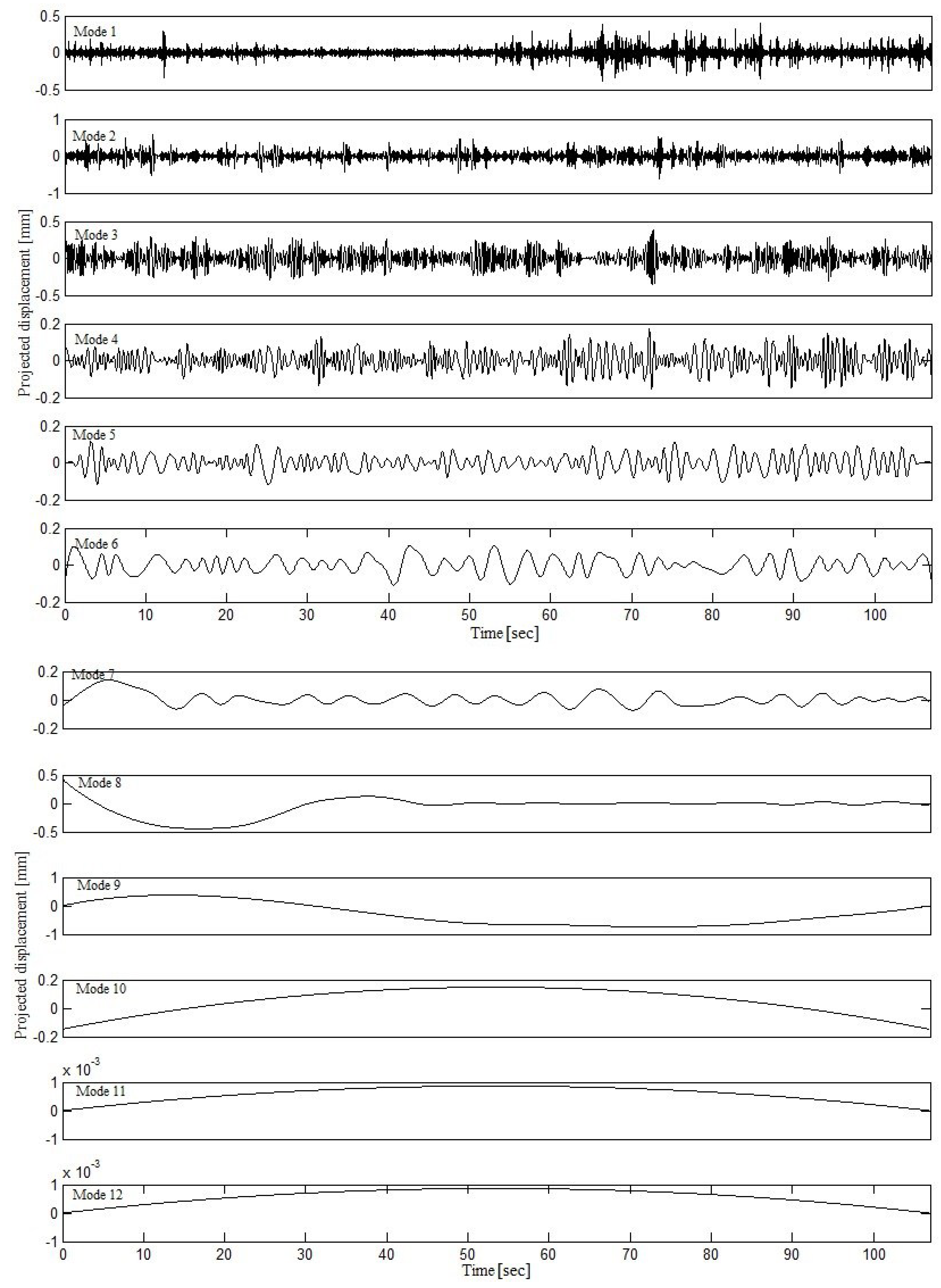
Figure 11.
Frequency distributions of eight modes of each set of time series displacements obtained by the direct interpolation algorithm. (a) Frequency distribution of each mode of point Rbin46_N; (b) Frequency distribution of each mode of point Rbin46_L; (c) Frequency distribution of each mode of point Rbin64_N; (d) Frequency distribution of each mode of point Rbin64_L.
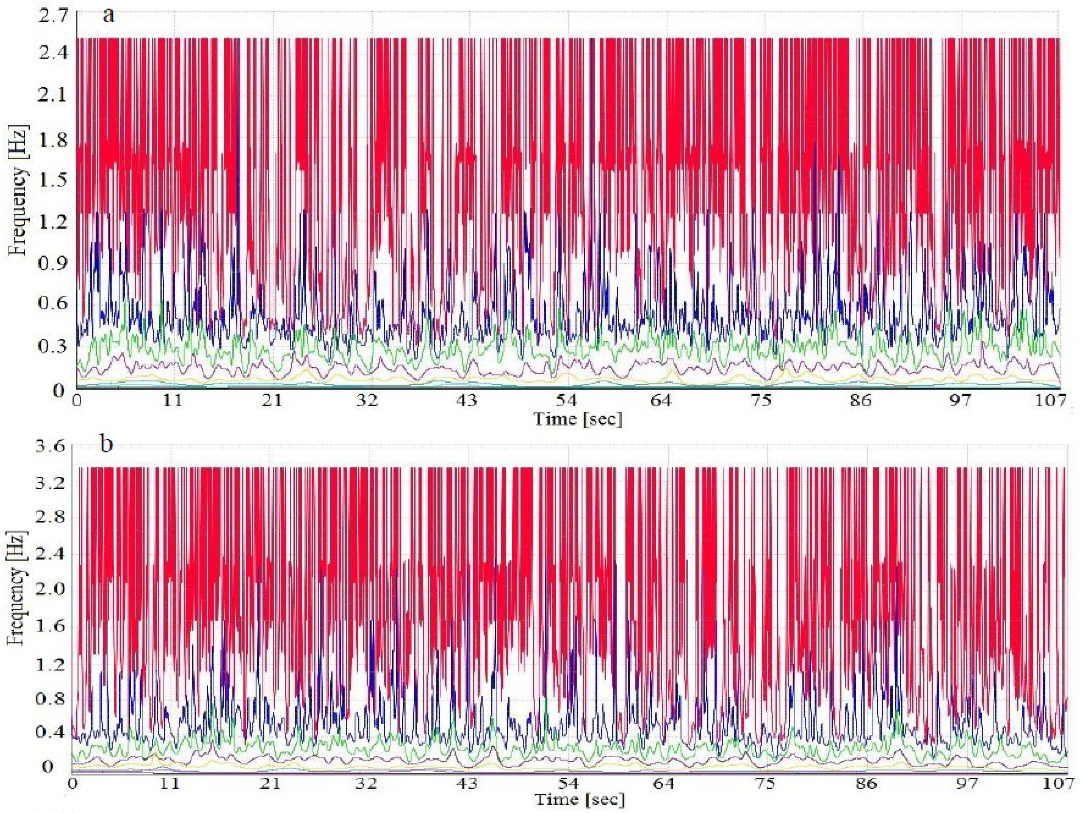

Figure 12.
Instantaneous frequency and amplitude of Mode 1 decomposed via the ESMD method for time series displacements by the direct interpolation algorithm. (a) Instantaneous frequency and amplitude of Mode 1 of point Rbin46_N; (b) Instantaneous frequency and amplitude of Mode 1 of point Rbin46_L; (c) Instantaneous frequency and amplitude of Mode 1 of point Rbin64_N; (d) Instantaneous frequency and amplitude of Mode 1 of point Rbin64_L.
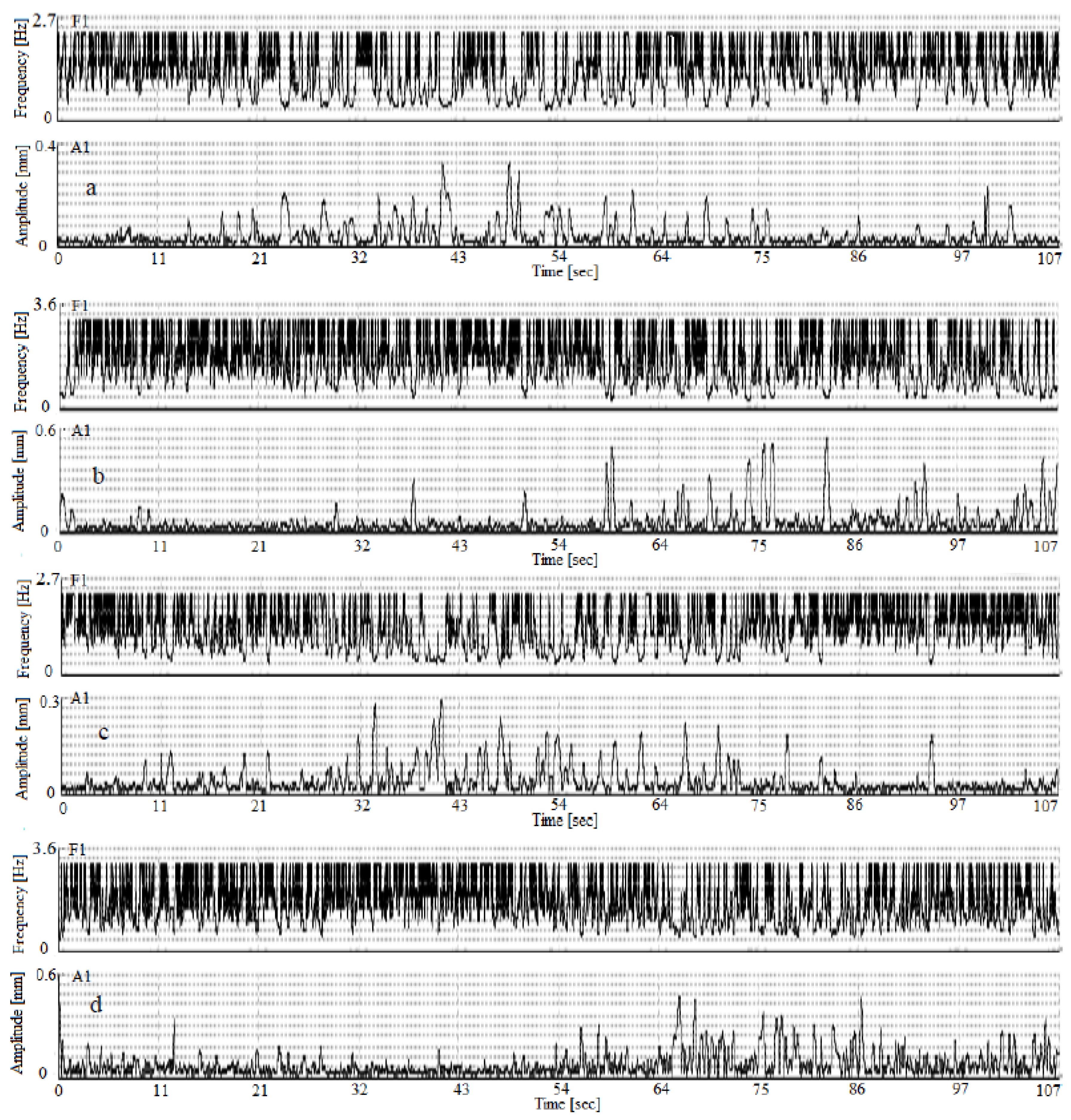
Figure 13.
Instantaneous frequency of Mode 1 of point Rbin64_L obtained by HHT.

Table 1.
Parameters of IBIS-S for the dynamic time series displacements acquisition of Zhaozhou Bridge.
Table 1.
Parameters of IBIS-S for the dynamic time series displacements acquisition of Zhaozhou Bridge.
| Parameter | Test 1 | Test 2 |
|---|---|---|
| Maximum distance | 200 m | 200 m |
| Working frequency | 16.6–16.9 GHZ | 16.6–16.9 GHZ |
| Range resolution | 0.5 m | 0.5 m |
| Sampling rate | 199.17 Hz | 199.17 Hz |
| Duration | 00:02:45 | 00:01:47 |
| Excitation condition | Environmental excitation | Transient loads |
Table 2.
The minimum variance ratios and the corresponding sifting times of the four kinds of time series displacements.
Table 2.
The minimum variance ratios and the corresponding sifting times of the four kinds of time series displacements.
| Point Name | Minimum Variance Ratio | Sifting Time (Number of Times) |
|---|---|---|
| Rbin46_N | 86.8% | 11 |
| Rbin46_L | 84.7% | 8 |
| Rbin64_N | 82.4% | 10 |
| Rbin64_L | 62.5% | 14 |
Table 3.
Parameters of the quality assessment for the frequency distribution of each set of time series displacements.
Table 3.
Parameters of the quality assessment for the frequency distribution of each set of time series displacements.
| Point | Parameter | F1 | F2 | F3 | F4 |
|---|---|---|---|---|---|
| Rbin46_N | MN (Hz) | 2.413 | 0.716 | 0.313 | 0.146 |
| SD (Hz) | 0.348 | 0.297 | 0.149 | 0.053 | |
| CV (%) | 14.4 | 41.5 | 47.6 | 36.3 | |
| Rbin46_Y | MN (Hz) | 3.362 | 0.901 | 0.391 | 0.207 |
| SD (Hz) | 0.582 | 0.379 | 0.184 | 0.074 | |
| CV (%) | 17.3 | 42.1 | 47.1 | 35.7 | |
| Rbin64_N | MN (Hz) | 2.422 | 0.715 | 0.314 | 0.145 |
| SD (Hz) | 0.351 | 0.296 | 0.151 | 0.053 | |
| CV (%) | 14.5 | 41.4 | 48.1 | 36.6 | |
| Rbin64_Y | MN (Hz) | 3.359 | 0.904 | 0.393 | 0.209 |
| SD (Hz) | 0.598 | 0.382 | 0.186 | 0.075 | |
| CV (%) | 17.8 | 42.3 | 47.3 | 35.9 |
© 2018 by the authors. Licensee MDPI, Basel, Switzerland. This article is an open access article distributed under the terms and conditions of the Creative Commons Attribution (CC BY) license (http://creativecommons.org/licenses/by/4.0/).
Share and Cite
MDPI and ACS Style
Liu, X.; Lu, Z.; Yang, W.; Huang, M.; Tong, X. Dynamic Monitoring and Vibration Analysis of Ancient Bridges by Ground-Based Microwave Interferometry and the ESMD Method. Remote Sens. 2018, 10, 770. https://doi.org/10.3390/rs10050770
AMA Style
Liu X, Lu Z, Yang W, Huang M, Tong X. Dynamic Monitoring and Vibration Analysis of Ancient Bridges by Ground-Based Microwave Interferometry and the ESMD Method. Remote Sensing. 2018; 10(5):770. https://doi.org/10.3390/rs10050770
Chicago/Turabian StyleLiu, Xianglei, Zhao Lu, Wanxin Yang, Ming Huang, and Xiaohua Tong. 2018. "Dynamic Monitoring and Vibration Analysis of Ancient Bridges by Ground-Based Microwave Interferometry and the ESMD Method" Remote Sensing 10, no. 5: 770. https://doi.org/10.3390/rs10050770
Note that from the first issue of 2016, this journal uses article numbers instead of page numbers. See further details here.