Geostationary Sensor Based Forest Fire Detection and Monitoring: An Improved Version of the SFIDE Algorithm

Abstract

The paper aims to present the results obtained in the development of a system allowing for the detection and monitoring of forest fires and the continuous comparison of their intensity when several events occur simultaneously—a common occurrence in European Mediterranean countries during the summer season. The system, called SFIDE (Satellite FIre DEtection), exploits a geostationary satellite sensor (SEVIRI, Spinning Enhanced Visible and InfraRed Imager, on board of MSG, Meteosat Second Generation, satellite series). The algorithm was developed several years ago in the framework of a project (SIGRI) funded by the Italian Space Agency (ASI). This algorithm has been completely reviewed in order to enhance its efficiency by reducing false alarms rate preserving a high sensitivity. Due to the very low spatial resolution of SEVIRI images (4 × 4 km² at Mediterranean latitude) the sensitivity of the algorithm should be very high to detect even small fires. The improvement of the algorithm has been obtained by: introducing the sun elevation angle in the computation of the preliminary thresholds to identify potential thermal anomalies (hot spots), introducing a contextual analysis in the detection of clouds and in the detection of night-time fires. The results of the algorithm have been validated in the Sardinia region by using ground true data provided by the regional Corpo Forestale e di Vigilanza Ambientale (CFVA). A significant reduction of the commission error (less than 10%) has been obtained with respect to the previous version of the algorithm and also with respect to fire-detection algorithms based on low earth orbit satellites.

1. Introduction

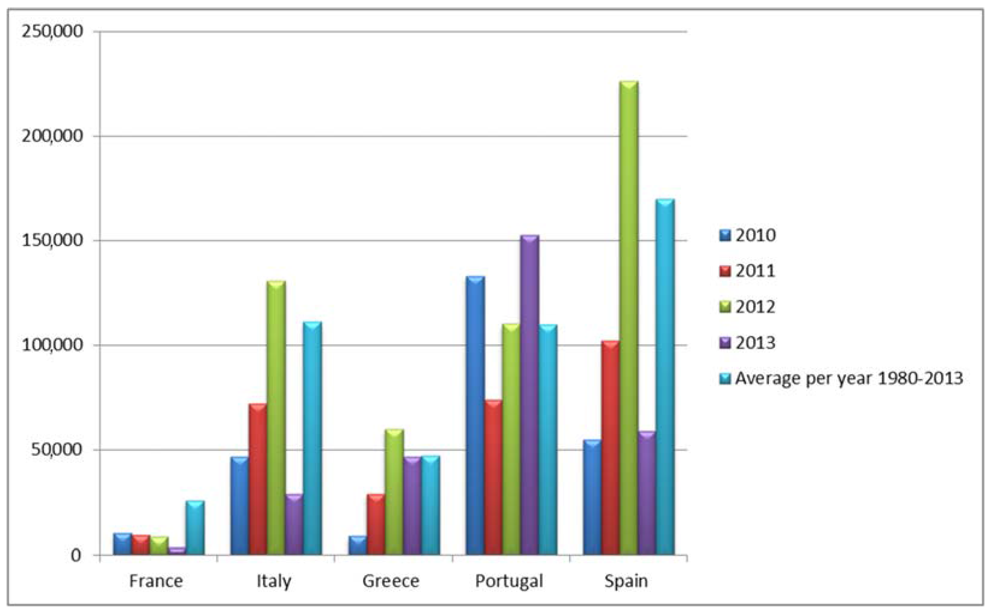
Every year, annual reports highlight the extent of the forest fires phenomenon in the European Union, where more than half a million ha of forests burn in about 65,000 fires (Figure 1) [1,2]. This phenomenon is particularly relevant in the European Mediterranean region, where climatic factors produce a high level of vegetation stress during the summer months which causes a higher risk of inflammability.

In Italy, the amount of wildland and forest areas that burns each year is, on average, 50,000 ha, and this phenomenon is particularly relevant in regions such as Sardinia, where, from 1995 to 2009, an area of 16,600 ha per year burnt, and over 90% of these fires were human-induced [3].

For this reason, the adoption of a system capable of detecting as early as possible the trigger of new fires would considerably reduce environmental, material and social damage [4].

The use of satellite systems (NOAA/AVHRR, GOES, etc.), developed in the early 1970s by the US Forest Service [5], can be an extraordinary tool to detect hotspots and evaluate vegetation stress level.

A first classification of fire detection algorithms using remote data, distinguishes between those in which information is provided by a single channel (one-channel algorithms), and those in which data are provided from two or more channels (multi-channel algorithms). In both cases, it is essential to have information in the MWIR (Medium Wave InfraRed) region of the spectrum, and in particular in channels around 3.9 μm: the radiative emission peak for temperatures that characterize forest fires (800–1500 K) is in the range of 2–4 μm and, moreover, it is possible to work in atmospheric windows. In the case of multi-channel systems, it is common practice to choose a second channel in the TIR (Thermal InfraRed) region, at wavelengths between 8 μm and 12 μm, where the emission of bodies at temperatures close to those characterizing the Earth’s surface is maximum, as in Dozier [6].

Most of the current multi-channel algorithms use band at 3.9 μm in combination with band at 10.8 μm, available for the major satellite sensors used for fire detection. Remote data in these channels are often accompanied by the VIS (VISible) bands, used for the detection of pixels with cloud coverage and for the detection of false alarms.

A further distinction concerning fire detection systems is based on the characteristics of the orbit in which the satellite is located. For low orbit, the advantage of having images at a higher spatial resolution is accompanied by a low frequency of observation (approximately, two observations per day). Using instead weather satellites located in geostationary orbit, it is possible to have a continuous monitoring (images are usually acquired every 15’ or 30’), but with a significantly lower spatial resolution (from 3 to 5 km per pixel, depending on latitude). Despite the disadvantages of low spatial resolution as the minimum dimensions of detectable fires, this last solution is useful for the purpose of real-time monitoring.

MODIS (Moderate Resolution Imaging Spectroradiometer) and AVHRR (Advanced Very High Resolution Radiometer) are among the most commonly used low orbit satellite sensors for forest fire monitoring. In the last few years (2013), the new generation medium resolution imager, the VIIRS (Visible Infrared Imaging Radiometer Suite) satellite sensor, has been used to detect active fires, also.

MODIS radiometer allows the detection of data in 36 spectral bands from VIS to TIR with resolution of 250 m for channels 1–2, 500 m for channels 3–7, and 1 km for the remaining bands. MODIS sensors are located on NASA Aqua and Terra satellites. These two complementary satellites, allow the detection of images of the same region four times per day, recording two images during diurnal hours and two during nocturnal hours [7]. The works of Kaufman [8], Justice [9] and Giglio [10,11,12] are the most relevant for fire detection using MODIS data. AVHRR/3 is the third and last generation of the radiometer developed by NOAA (National Oceanic and Atmospheric Administration) in collaboration with NASA, used since 1978. It has 6 radiometric channels with 1 km resolution, and its orbit permits the acquisition of one or two images of the same area per day.

For fire detection using AVHRR data, the works of Robinson [13], Flasse and Ceccato [14] and Giglio [11,15] are of primary importance. The VIIRS sensor on the Suomi National Polar-orbiting Partnership (S-NPP) satellite incorporates fire-sensitive channels enabling active fire detection and characterization [16]. Concerning geostationary satellites: the works of Prins [17], Reid [18] and Xu [19] are most relevant for fire detection using GOES (Geostationary Operational Environmental Satellite) radiometer whereas the present work is focused on the images of the MSG satellite series, operated by EUMETSAT consortium. The SEVIRI (Spinning Enhanced Visible and Infrared Imager) sensor on board of MSG satellite can acquire images every 15 min, in twelve channels: three in Visible and Near Infra-Red (VNIR), and eight in Infra-Red (IR). These images have 3 km resolution at the sub-satellite point (the equator), with the exception of the High Resolution Visible (HRV) channel (12th), which provides 1 km resolution images [20].

For fire detection using MSG-SEVIRI data, works of Calle [21], Laneve [22], Roberts and Wooster [23] and Amraoui [24] are relevant. Calle proposes an algorithm capable of detecting fire with a minimum dimension of 0.7 ha on the Iberian land; Laneve shows a process for real-time coverage in Mediterranean area; Roberts and Wooster propose an algorithm in which false detection is less than 4% of observed fires; lastly, Amraoui proposes an algorithm for live coverage and combusted area rates on Africa.

Mediterranean areas are at the highest risk and suffer great losses of infrastructures, forested and agricultural land, human and livestock lives. The risk of such fires is expected to increase in forthcoming years under the impact of climate changes; vegetation becomes more inflammable (due to thermal stress and drought) and fire services are faced with difficulties when trying to suppress a fire due to increased inflammability and water shortage [4].

Previous studies demonstrate the capabilities of SEVIRI to detect fires, despite its low spatial resolution. In the Mediterranean areas thanks to its geostationary orbit, it can drastically reduce the reaction times compared to fire-detection based on low orbit systems. The main purpose of this paper is to show the utility of geostationary systems (MSG/SEVIRI) for fire-detection, focusing on fire occurrences on the Sardinian island, characterized by a non-homogeneous coverage (that is, the coexistence of urban settlements, infrastructure networks and vegetated areas (forest, agricultural and uncultivated areas) in a complex, dense and intricate patchwork) and high anthropization, issues neglected by current literature. In 2008, SIGRI (Sistema Integrato per la Gestione del Rischio Incendi) project was funded by ASI (Agenzia Spaziale Italiana) to face natural and human-induced disaster, and to demonstrate the abilities of supporting risk assessment, monitoring and management of fire by using remote-sensing satellite systems [25,26,27].

SEVIRI sensor is showing its ability to guarantee a live coverage by sending data every fifteen minutes. The CRPSM (Centro di Ricerca Progetto San Marco) has been studying for several years the possibility of using images acquired by SEVIRI: SFIDE (System for FIre DEtection) algorithm, presented in this paper, has been developed to exploit the images high update frequency by comparing temperature variation in subsequent images (change-detection), by using thresholds fit on the Sardinian island.

The paper is organized as follows: Section 2.1 describes exploited data and method for real time coverage, Section 2.2 describes SFIDE algorithm; Section 3 shows the results achieved by comparing hot spots detected by SFIDE, ground data provided by forest rangers CFVA (Corpo Forestale e di Vigilanza Ambientale) and hot spots detected by low orbit based fire-detection system.

2. Data and Methodology

The most common algorithms developed in the last decade, use remote data from low orbit satellite sensors (MODIS, AVHRR) or geostationary orbit satellite sensor (SEVIRI, GOES Imager) to apply absolute thresholds or contextual tests and obtain hot-spots as output results, together with the characterization of the fire pixels. In Section 2.1 a model of fire-detection algorithm and a description of input data is shown; in Section 2.2 how SFIDE algorithm uses absolute and contextual tests together with an innovative change-detection method to obtain a continuous monitoring of interested area from geostationary orbit data is illustrated.

2.1. Data & Methods

The European MSG satellite series are geostationary meteorological satellites operated by the EUMETSAT consortium. The most important sensor for the purpose of this paper is SEVIRI, comprising 11 spectral bands and a visible broadband (HRV) [

Table 1. Bands of SEVIRI radiometer (www.esa.int).

Channel	Spectral Band	Wavelength (μm)	Central Wavelength (μm)	Equator Resolution (km)
1	VIS 0.6	0.56–0.71	0.635	3
2	VIS 0.8	0.74–0.88	0.81	3
3	IR 1.6	1.50–1.78	1.64	3
4	IR 3.9	3.48–4.36	3.92	3
5	WV 6.2	5.35–7.15	6.25	3
6	WV 7.3	6.85–7.85	7.35	3
7	IR 8.7	8.30–9.10	8.70	3
8	IR 9.7	9.38–9.94	9.66	3
9	IR 10.8	9.80–11.80	10.80	3
10	IR 12.0	11.00–13.00	12.00	3
11	IR 13.4	12.40–14.40	13.40	3
12	HRV	0.60–0.90	0.75	1

].

Main applications of SEVIRI scanner are [28]: cloud detection through VIS 0.6 and VIS 0.8 channels; aerosol, soil humidity and vegetation index retrieval (IR 1.6, VIS 0.6, VIS 0.8); water vapor and wind determination (IR 6.2, IR 7.3); clouds and their temperature (IR 3.8, IR 8.7, IR 10.8, IR 12.0); high-atmosphere monitoring (IR 9.7); pressure at high altitude (IR 13.4).

SFIDE algorithm uses IR 3.8, IR 10.8, IR 12.0, VIS 0.6, VIS 0.8 for fire detection and estimation of surface temperature.

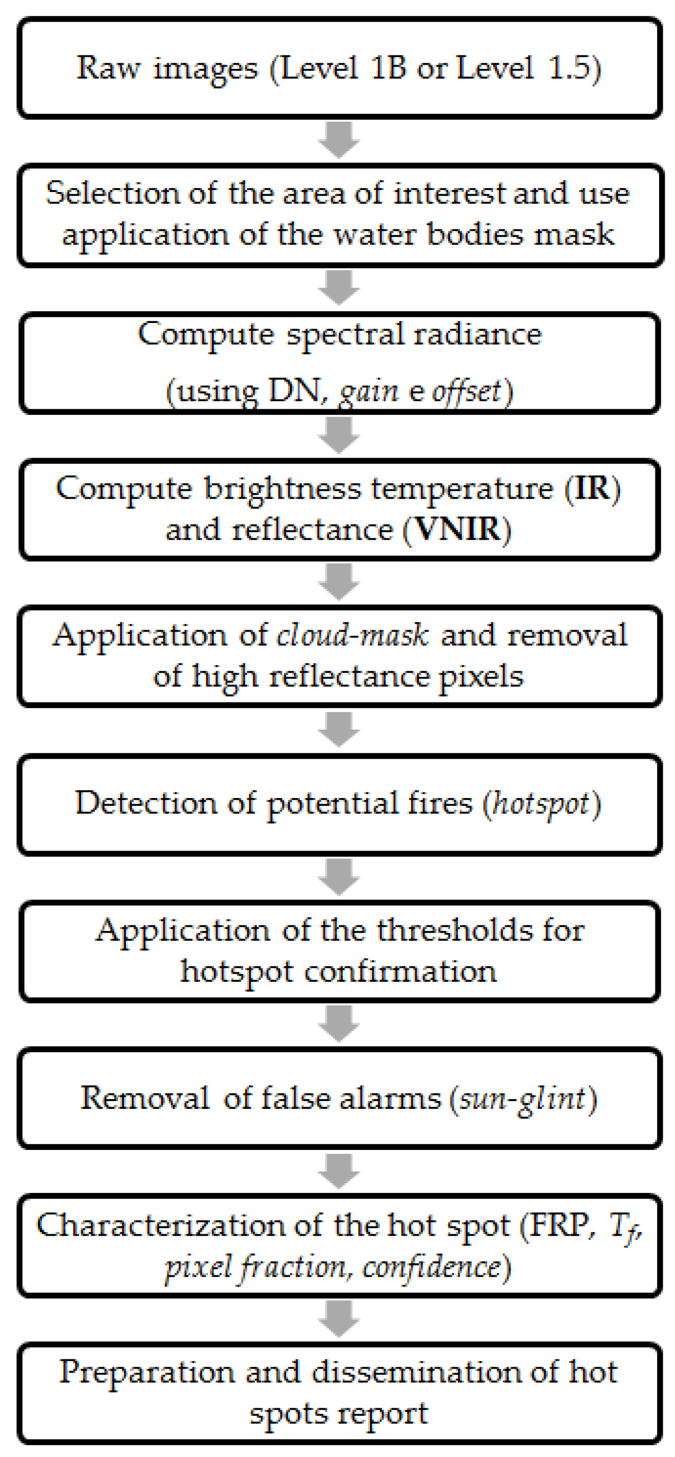
The common steps characterizing a fire-detection algorithm using remote sensing data are presented in Figure 2. The SEVIRI images are directly acquired at the University of Rome premises through the EUMETCAST service. After preliminary operations, consisting in the selection of interested area and the application of a sea-mask to exclude pixels in sea area, the brightness temperature (T_b) is evaluated whereas reflectance (r_ch) in VIS channels is retrieved knowing the values of radiance (R), Digital Number (DN), calibration coefficient (c_f) and Offset (R₀), data contained in the heading of SEVIRI images, archived in pgm (portable gray map) format.

One of the most common causes of false alarm in fire detection is the presence of clouds within the pixel, as clouds have similar features to fires: increase of T_b in MIR channel at 3.9 μm (T_b3.9) due to a major reflection of sunlight, decrease of T_b in TIR channel at 10.8 μm (T_b10.8), a consequent increase of brightness temperature difference (ΔT) between 3.9 μm and 10.8 μm channel. Various methods are adopted to detect cloud pixels. An algorithm similar to the one proposed by Saunders and Kriebel for AVHRR sensor [29] will be employed in this work. The algorithm applies fixed thresholds and distinguishes daily and nightly hours.

It is now possible to detect hot spots by applying specific thresholds. Using fixed thresholds for T_b3.9 and for ΔT, it is possible to distinguish two categories of pixels: non-fire pixel or potential-fire pixels. This distinction is generally made by using a multi-channel approach with fixed thresholds. A pixel is considered a potential hot-spot if it satisfies:

$$\{\begin{array}{l}{T}_{b3.9}>T_{b3.9}{}_{MIN}\\ \mathit{\Delta }T=T_{b3.9}-T_{b10.8}>\mathit{\Delta }{T}_{min}\end{array}$$

(1)

where T_b3.9MIN and ΔT_min are threshold values of T_b3.9 and ΔT, specifically selected considering vegetation coverage. Official reports by EUMETSAT [28] apply as fixed thresholds for a potential fire-pixel: 310 K and 5 K for daytime hours and 290 K and 0 K for nocturnal hours. In the last few years, a dependence on solar elevation, or solar zenith angle (SZA) has been shown. This condition allows the avoidance of omission errors in the hours in which SZA is higher.

Fixed thresholds expressed as linear function of SZA are:

$$\{\begin{array}{l}{T}_{b3.9}>T_{b3.9}{}_{\_0}-c_{3.9}\times SZA\\ \mathit{\Delta }T=T_{b3.9}-T_{b10.8}>\mathit{\Delta }{T}_0-c_{\mathit{\Delta }T}\times SZA\end{array}$$

(2)

where T_{b3.9_0} and ΔT₀ are constants chosen for SZA = 0°; c_3.9 and c_ΔT are coefficients evaluated as 0.3 [K/deg] and 0.0049 [K/deg] [23].

The algorithm usually continues by applying contextual thresholds, in some cases used for the validation of fire points [19,23], in other cases used as test for hot-spot detection [8,15]. Contextual algorithm is based on average values of $T_{b3.9}$, $\mathit{\Delta }T$ and their standard deviations (${\delta }_T{}_{{}_{b3.9}}$ e ${\delta }_{\mathit{\Delta }T}$) in $n\times n$ regions centered on the supposed fire point (from 3 × 3 to 5 × 5 pixels in case of GEO-Geostationary Earth Orbit-satellite based systems, to 21 × 21 pixels for LEO-Low Earth Orbit-satellite). Thresholds for the detection of fire points are:

$$\{\begin{array}{l}{T}_{b3.9}>\overline{T_{b3.9}}+k_{T_{b3.9}}\cdot {\delta }_{T_{b3.9}}-k_0\\ \mathit{\Delta }T>\overline{\mathit{\Delta }T}+\max (k_{\mathit{\Delta }T}\cdot {\delta }_{\mathit{\Delta }T},\mathit{\Delta }{T}_{MIN})\end{array}$$

(3)

where $\overline{T_{b3.9}}$ and $\overline{\mathit{\Delta }T}$ are average values of $T_{b3.9}$ and $\mathit{\Delta }T$ in $n\times n$ region; $k_{T_{b3.9}}$ and $k_{\mathit{\Delta }T}$ are dimensionless coefficients with values ranging from 2 to 4; $k_0$ is a constant between 0 K and 3 K; $\mathit{\Delta }{T}_{MIN}$ is a constant between 2.5 K and 6 K; $\max (k_{\mathit{\Delta }T}\cdot {\delta }_{\mathit{\Delta }T},\mathit{\Delta }{T}_{MIN})$ is an operator that returns the maximum value between $k_{\mathit{\Delta }T}\cdot {\delta }_{\mathit{\Delta }T}$ and $\mathit{\Delta }{T}_{MIN}$. Giglio suggests for MODIS sensor: $k_{T_{b3.9}}=3$, $k_{\mathit{\Delta }T}=3.5$, $k_0=0$ K, $\mathit{\Delta }{T}_{MIN}=6$ K [12]. Robert and Wooster suggest for SEVIRI sensor:$k_{T_{b3.9}}=2$, $k_{\mathit{\Delta }T}=2$, $k_0=0$ K, $\mathit{\Delta }{T}_{MIN}=2.5$ K [23].

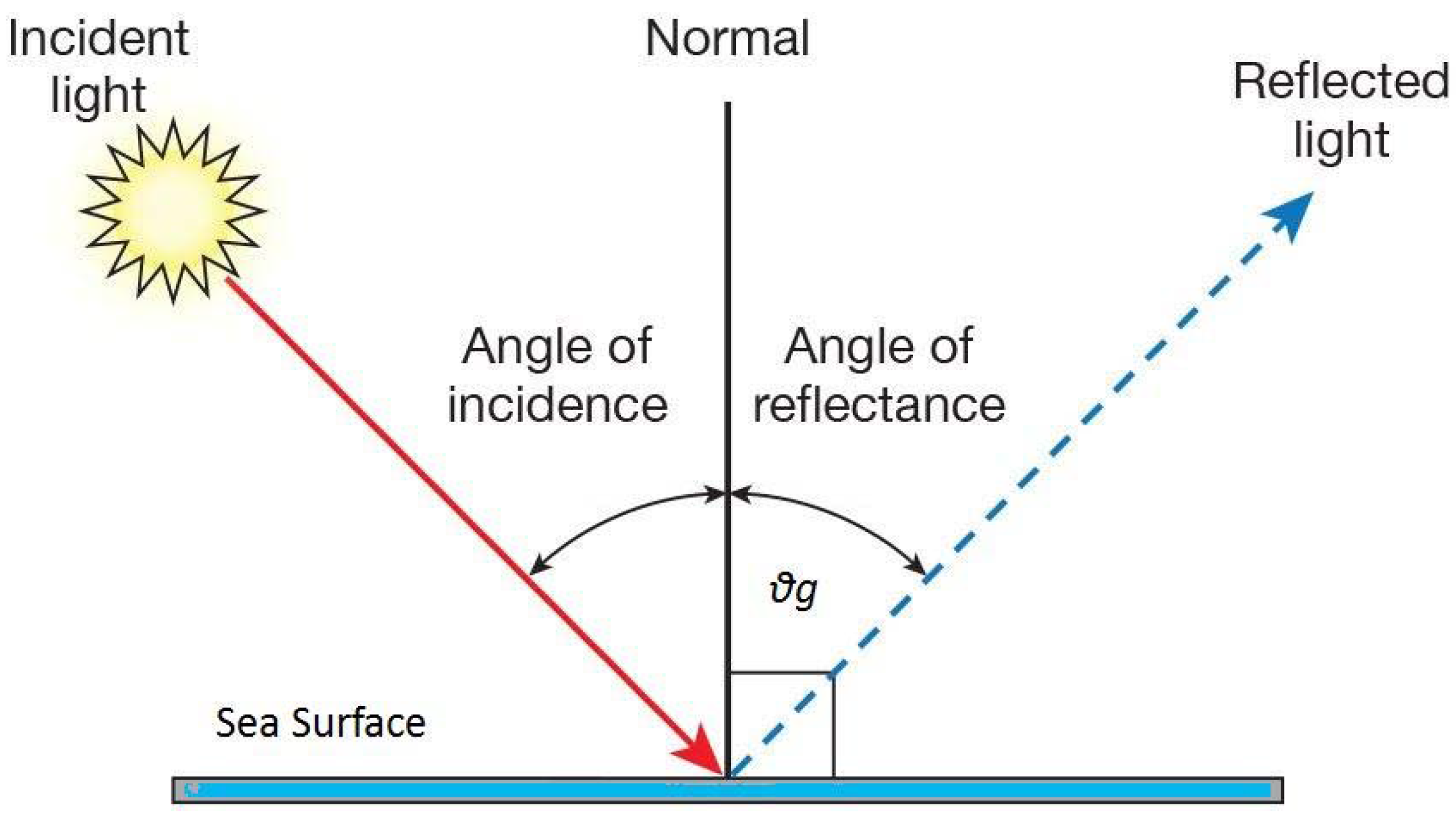
A further cause of false alarm is the sun-glint phenomenon, or the reflection of sunlight on water mirrors that causes an increase of $T_{b3.9}$ and $\mathit{\Delta }T$. If there is a correspondence between the angle value (${\vartheta }_g$) between the line connecting surface-satellite and the specular direction to the solar radiation affecting the water mirror (Figure 3), then high risk for coast line pixels occurs.

Even if water bodies are excluded from the analysis by applying a mask, the phenomenon could occur at water-land border pixels. This is particularly evident in GEO systems due to their low resolution, and it is given by ground and water co-presence in the same pixel, that lead to a contamination of the contextual algorithm.

More selective thresholds or further tests are therefore used for coast line pixels. Giglio [12] suggests for MODIS satellite:

$$\{\begin{array}{c}{\vartheta }_g<2^{°}\\ \begin{array}{c}or\\ {\vartheta }_g<{10}^{°}\mathrm{and}{r}_{0.6}>0.1 and r_{0.8}>0.2 and r_{2.1}>0.12\\ or\end{array}\\ {\vartheta }_g<{15}^{°}\mathrm{and}{N}_w>0\end{array}$$

(4)

where $r_{2.1}$ is the reflectance at 2.1 µm (channel 7); $N_w$ is the number of sea-pixels in 3 × 3 grid.

Hot-spots detected are now characterized in terms of dimensions (fire size in each pixel, $\rho$, and $A_f=\rho A_{PIXEL}$, where $A_{PIXEL}$ is the area of a pixel [m²]), fire temperature ($T_f$), FRP (Fire Radiative Power) and confidence level of the fire point.

Dimension and temperature of fire can be obtained by the two-channel approach (at 3.9 µm and 10.8 µm) proposed by Dozier [6], based on the estimation of the radiant components of the pixel in absence of fire. Since the Dozier algorithm is based on a system of equations in two variables the active surface area can be estimated if the emissivity of the fire is known, otherwise we can determine their product.

FRP and its integration over time, FRE (Fire Radiative Energy), are further characterizations to estimate burned biomass of the pixel. In a first, two-channel approach, after solving equations proposed in [6], $T_f$ and $\rho$ are obtained and it is possible to evaluate the Fire Radiative Power using Stefan–Boltzmann law [30]:

$$FR{P}_{SB}=A_f\cdot {\epsilon }_f\cdot \sigma \cdot \left(T_f^4-T_b^4\right)$$

(5)

where $FR{P}_{SB}$ is fire radiative power estimated by Stefan–Boltzmann in [W]; ${\epsilon }_f$ is the emissivity of $A_f$; $\sigma$ is Stefan–Boltzmann constant.

Another approach is offered by Wooster equation [31], and it does not require values of $T_f$ and $\rho$:

$$FR{P}_W=\frac{A_{PIXEL}\cdot \sigma \cdot {\epsilon }_f}{a\cdot {\epsilon }_{f,3.9}}{L}_{3.9}$$

(6)

where $FR{P}_W$ is fire radiative power estimated by Wooster in [W]; ε_f is the emissivity of the fire and ε_f,3.9 is spectral emissivity at about 3.9 μm, a is a typical constant dependent from used sensor (a = 3.06 × 10⁻⁹ for SEVIRI). In Wooster et al. [31] gray body behavior is assumed, that is (ɛ_f = ɛ_f,3.9).

After estimating FRP using described methods, it is possible to evaluate FRE by integrating FRP over time:

$$FRE={\displaystyle \underset{t_{fire}}{\int }FRPd}t$$

(7)

where $t_{fire}$ is the fire duration.

Using the following equation, the estimation of burned biomass (BB) is obtained [23]:

$$BB\cong C_r\cdot FRE$$

(8)

where C_r is a conversion factor that links the FRP to combustion rate. In Wooster et al. [31] a universal value of $C_r=0.368$ [kg/MJ] is proposed, while Kaiser et al. [32] proposed specific values for different land cover classes. Combusted biomass density (${\rho }_B$) is [31]:

$${\rho }_B\cong \frac{BB}{A_f}$$

(9)

Finally, it is possible to estimate a quality index of hot-spot which takes into account the amount of clouds in the area of interest and their position with respect to the hot spot. Current literature provides further heuristic methods able to estimate confidence level (C) of each hotspot, as the one proposed by Giglio for MODIS [10,12] or the ones proposed by Roberts and Wooster [23] and Xu et al. [19] for GOES.

The data used to validate the results of the algorithm herein described include:

• Fire events reported by CFVA (Corpo Forestale e di Vigilanza Ambientale) of the Sardinia Region, that is the agency involved in the fire-fighting;
• Hot spots detected by the MODIS and VIIRS satellite sensors.

2.2. The SFIDE Algorithm

In this section SFIDE algorithm and its innovative aspects are described. It is important to highlight that the algorithm has been developed to be efficient in Mediterranean areas and, in particular, validation tests have been carried out in Sardinia. The complexity of the area of interest, because of its non-homogeneous and anthropized coverage, led to the elaboration of different conditions compared to the ones used in current literature.

Because of its objective to perform real time monitoring using geostationary satellite, one of the innovation of SFIDE algorithm consists in fire detection based on change-detection thresholds, evaluated at 15 min and 30 min intervals. Anomalous variations of $T_{b3.9}$ and $\mathit{\Delta }T$ in these intervals are considered as a sign of new fire event.

Further innovation is the introduction of thresholds which aim at detecting fire pixels using statistical analysis of $T_{b3.9}$ and $\mathit{\Delta }T$ as function of SZA: false alarms due to fixed thresholds have been overcome, as well as the ones due to linearly dependent thresholds by SZA.

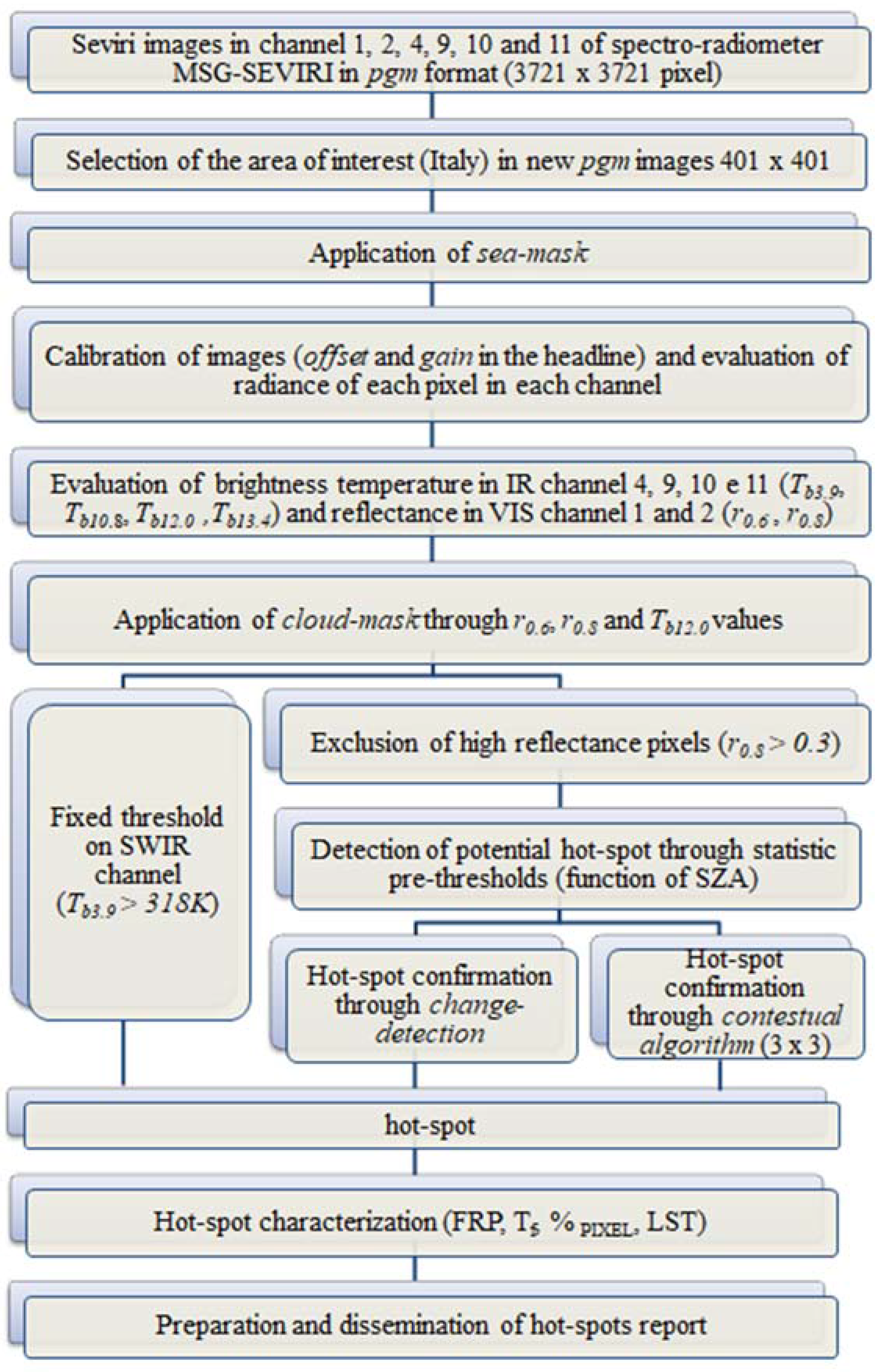
The SFIDE algorithm prospect for diurnal data analysis (SZA < 85°) is shown in Figure 4. Principal steps of the algorithm are the following:

• Preliminary operations and applications of masks;
• Fixed thresholds;
• Potential hot-spot detection;
• Hot-spot confirmation;
• Hot-spot characterization.

2.2.1. Preliminary Operations

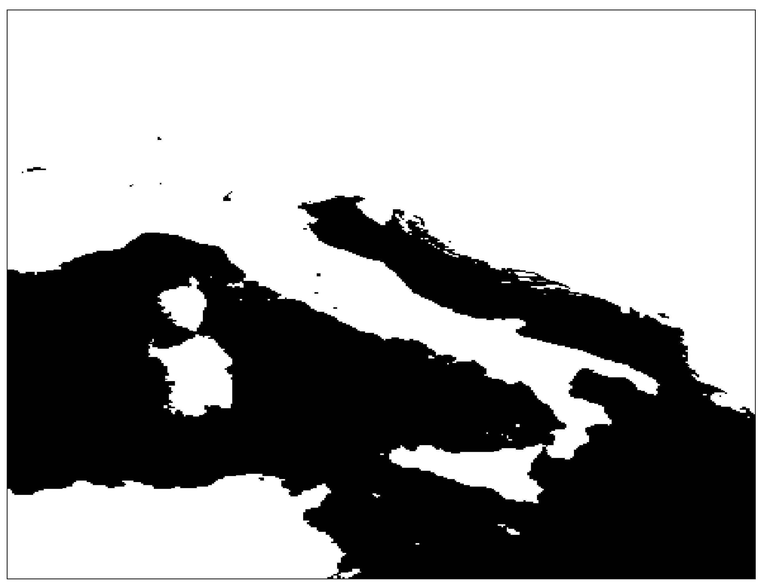
The first significant stage consists of applying typical preliminary operation: the selection of the area of interest, application of the sea-mask (Figure 5) and transformation of the DN (Digital Number) in radiances and then in reflectances (channels 1, 2) and brightness temperatures (channels 4, 9, 10, 11).

The next step is the application of a cloud-mask including new thresholds appropriately modified to be applied to Sardinia, as the introduction of thresholds on channel 2 and its relative reflectance ($r_{0.8}$). Similarly to [29], a pixel is considered as cloud covered if it satisfies:

$$\{\begin{array}{c}{r}_{0.6}+ r_{0.8}>1\\ \begin{array}{c}\mathrm{or}\\ T_{b12.0}<265 K\\ \mathrm{or}\end{array}\\ r_{0.6}+r_{0.8}>0.7 and{T}_{b12.0}<285 \mathrm{K}\end{array}$$

(10)

Other pixels, even not masked as cloudy could be excluded by the algorithm because of their high reflectance.

Reflectance in channel 2 is also used to exclude partly covered pixels because of their high reflectance, which could cause false alarms, and also pixels that satisfy:

$$r_{0.8}>0.35$$

(11)

are excluded.

Value in Equation (11) is more flexible than the one proposed in [15] to reduce omission errors due to the exclusion of elevated reflectance pixels.

The importance of excluding cloudy pixels will be shown again in the step of hotspot confirmation.

2.2.2. Fixed Thresholds

Omission errors can occur when both (10) and (11) are implemented; to avoid this, a fixed threshold has been imposed on :

$$T_{b3.9}>318K$$

(12)

Pixels that satisfy (12) are classified as hot-spots. Temperature of 318 K has been chosen after analysis of $T_{b3.9}$ trend in the considered area. An investigation of seasonal trend of $T_{b3.9}$ in the study area showed that all pixels that satisfies (12), together with adequate values of FRP (see next), has been validated as fire-pixels. As shown in Figure 4, this represents the first test used to detect hot-spots.

2.2.3. Potential Hot-Spot Detection

Two kinds of thresholds are used to detect hot-spots: fixed thresholds and SZA dependent thresholds. Thresholds expressed as linear function of SZA are generally preferred to the fixed ones, but omission and commission errors are not avoided. To model with more accuracy the average values of $T_{b3.9}$ and $\mathit{\Delta }T$, an analysis of their average trend as function of SZA on Sardinia has been conducted. Their trend and their standard deviation have been stored and described by a third-degree function, used as potential hot-spot detection threshold. Obtained functions are:

$$\langle T_{b3.9}\rangle =\mp {6.2410}^{-6}·SZ{A}^3-0.0027·SZ{A}^2\pm 0.052·SZA+305.43$$

(13)

$$\langle \mathit{\Delta }T\rangle =\mp {4.7510}^{-6}·SZ{A}^3-0.0011·SZ{A}^2\pm 0.018·SZA+3.69$$

(14)

where $\langle T_{b3.9}\rangle$ and $\langle \mathit{\Delta }T\rangle$ are respectively expected values of $T_{b3.9}$ and $\mathit{\Delta }T$ as a function of SZA. In the terms with odd exponent, the use of superior sign is for post-meridian hours, and inferior sign is for anti-meridian hours. A pixel is considered a hot-spot if it satisfies:

$$\{\begin{array}{l}{T}_{b3.9}>\langle T_{b3.9}\rangle \\ \mathit{\Delta }T=T_{b3.9}-T_{b10.8}>\langle \mathit{\Delta }T\rangle \end{array}$$

(15)

2.2.4. Hot-Spot Confirmation

At this stage, checks on potential hot-spots are carried out to confirm them. Checks follow two paths: change-detection and contextual analysis. For both methodologies, narrower thresholds have been used for high false alarm risk pixel due to its partial cloud coverage, sudden change in reflection over time, or Sun-glint.

Change-detection: This innovative approach is particularly efficient in detecting new fires earlier than contextual analysis. Statistical analysis has been conducted on average trend of T_b3.9 and ΔT as function by SZA at 15 and 30 min intervals. Data on their average variations have been interpolated in third degree function dependent on SZA and used as pre-thresholds. Lastly, these functions have been used to evaluate a kind of thresholds, named trigger thresholds, that allow one to confirm fires in growing phase because of the joint increase of T_b3.9 and ΔT above statistically evaluate values.

The following symbolism has been used:

• T_{b3.9_15’} and ΔT_15’: T_b3.9 and ΔT values for image that precedes by 15 min the current one;
• T_{b3.9_30’} and ΔT_30’: T_b3.9 and ΔT values for image that precedes by 30 min the current one;
• ΔT_{b3.9_15’} = (T_b3.9 − T_{b3.9_15’}) and Δ(ΔT)_15’ = (ΔT − ΔT_15’): T_b3.9 and ΔT variations between current image and the one that precedes at 15 min;
• ΔT_{b3.9_30’} = (T_b3.9 − T_{b3.9_30’}) and Δ(ΔT)_30’ = (ΔT − ΔT_30’): T_b3.9 and ΔT variations between current image and the one that precedes at 30 min.

For the thermal variations of 15 min, evaluated as ΔT_{b3.9_15’} and Δ(ΔT)_15’ trend and their respective standard deviations are:

$$\langle \mathit{\Delta }{T}_{{b3.9\_15}^{\prime }}\rangle =\mp 2.91\mathrm{E}-7\cdot {\mathrm{SZA}}^3-1.75\mathrm{E}-5\cdot {\mathrm{SZA}}^2\pm 4.39\mathrm{E}-4\cdot \mathrm{SZA}+0.49$$

(16)

$$\langle {\sigma }_{\mathit{\Delta }{T}_{{b3.9\_15}^{\prime }}}\rangle =\pm 1.00\mathrm{E}-6\cdot {\mathrm{SZA}}^3-5.09\mathrm{E}-5\cdot {\mathrm{SZA}}^2\mp 1.77\mathrm{E}-2\cdot \mathrm{SZA}+0.21$$

(17)

$$\langle \mathit{\Delta }{(\mathit{\Delta }T)}_{{15}^{\prime }}\rangle =\pm 5.03\mathrm{E}-7\cdot {\mathrm{SZA}}^3-1.21\mathrm{E}-6\cdot {\mathrm{SZA}}^2\mp 6.84\mathrm{E}-3\cdot \mathrm{SZA}+0.005$$

(18)

$$\langle {\sigma }_{\mathit{\Delta }{(\mathit{\Delta }T)}_{{15}^{\prime }}}\rangle =\mp 7.17\mathrm{E}-7\cdot {\mathrm{SZA}}^3-8.81\mathrm{E}-5\cdot {\mathrm{SZA}}^2\pm 1.75\mathrm{E}-3\cdot \mathrm{SZA}+0.85$$

(19)

where $\langle \mathit{\Delta }{T}_{{b3.9\_15}^{\prime }}\rangle$ and $\langle \mathit{\Delta }{(\mathit{\Delta }T)}_{{15}^{\prime }}\rangle$ are functions that approximate the average trend of ΔT_{b3.9_15’} and Δ(ΔT)_15’, while $\langle {\sigma }_{\mathit{\Delta }{T}_{{b3.9\_15}^{\prime }}}\rangle$ and $\langle {\sigma }_{\mathit{\Delta }{(\mathit{\Delta }T)}_{{15}^{\prime }}}\rangle$ are functions that approximate their respective average standard deviations. Similarly, an analysis considering 30 min intervals has been conducted:

$$\langle \mathit{\Delta }{T}_{{b3.9\_30}^{\prime }}\rangle =\pm 1.95\mathrm{E}-6\cdot {\mathrm{SZA}}^3-1.25\mathrm{E}-4\cdot {\mathrm{SZA}}^2\mp 3.46\mathrm{E}-2\cdot \mathrm{SZA}+0.48$$

(20)

$$\langle {\sigma }_{\mathit{\Delta }{T}_{{b3.9\_30}^{\prime }}}\rangle =\mp 4.39\mathrm{E}-7\cdot {\mathrm{SZA}}^3-6.07\mathrm{E}-6\cdot {\mathrm{SZA}}^2\pm 1.21\mathrm{E}-3\cdot \mathrm{SZA}+0.75$$

(21)

$$\langle \mathit{\Delta }{(\mathit{\Delta }T)}_{{30}^{\prime }}\rangle =\pm 9.13\mathrm{E}-7\cdot {\mathrm{SZA}}^3-6.40\mathrm{E}-6\cdot {\mathrm{SZA}}^2\mp 1.34\mathrm{E}-2\cdot \mathrm{SZA}+0.026$$

(22)

$$\langle {\sigma }_{\mathit{\Delta }{(\mathit{\Delta }T)}_{{30}^{\prime }}}\rangle =\mp 1.18\mathrm{E}-6\cdot {\mathrm{SZA}}^3-1.09\mathrm{E}-4\cdot {\mathrm{SZA}}^2\pm 3.56\mathrm{E}-3\cdot \mathrm{SZA}+1.16$$

(23)

where $\langle \mathit{\Delta }{T}_{{b3.9\_30}^{\prime }}\rangle$ and $\langle \mathit{\Delta }{(\mathit{\Delta }T)}_{{30}^{\prime }}\rangle$ are functions that approximate the average trend of ΔT_{b3.9_30’} and Δ(ΔT)_30’, while $\langle {\sigma }_{\mathit{\Delta }{T}_{{b3.9\_30}^{\prime }}}\rangle$ and $\langle {\sigma }_{\mathit{\Delta }{(\mathit{\Delta }T)}_{{30}^{\prime }}}\rangle$ are functions that approximate their respective average standard deviations.

Functions described in Equations (16)–(23) are trigger thresholds imposed on potential hot-spots that satisfy Equation (15) to confirm fire in the pixel. Considering thermal variations in 15’, a potential hot-spot is confirmed if:

$$\{\begin{array}{l}\mathit{\Delta }{T}_{{b3.9\_15}^{\prime }}=(T_{b3.9}-T_{{b3.9\_15}^{\prime }})>\langle \mathit{\Delta }{T}_{{b3.9\_15}^{\prime }}\rangle +\langle {\sigma }_{\mathit{\Delta }{T}_{{b3.9\_15}^{\prime }}}\rangle \\ \mathit{\Delta }{(\mathit{\Delta }T)}_{{15}^{\prime }}=(\mathit{\Delta }T-\mathit{\Delta }{T}_{{15}^{\prime }})>\langle \mathit{\Delta }{(\mathit{\Delta }T)}_{{15}^{\prime }}\rangle +\langle {\sigma }_{\mathit{\Delta }{(\mathit{\Delta }T)}_{{15}^{\prime }}}\rangle +f_{{15}^{\prime }}(\mathit{\Delta }{r}_{0.6})\\ T_{b3.9}>\overline{T_{b3.9}}+1.5\\ \mathit{\Delta }T>\overline{\mathit{\Delta }T}+0.5\\ N_w+N_c=0\end{array}$$

(24)

where $\overline{T_{b3.9}}$ and $\overline{\mathit{\Delta }T}$ are average values of T_b3.9 and ΔT in 3 × 3 grid centered on potential hot-spots; N_w and N_c are respectively number of water-pixels and cloudy-pixels in 3 × 3 grid centered on potential hot-spots; $f_{{15}^{\prime }}(\mathit{\Delta }{r}_{0.6})=100(r_{0.6}-r_{{0.6\_15}^{\prime }})$ if $r_{0.6}>r_{{0.6\_15}^{\prime }}$, with $r_{{0.6\_15}^{\prime }}$ reflectance in channel 1 evaluated 15 min before current image. Function f_15’ is necessary to correct ΔT increase due to $r_{0.6}$ increase in 15’ intervals.

Considering thermal variations in 30’, a potential hot-spot is confirmed if it satisfies:

$$\{\begin{array}{l}\mathit{\Delta }{T}_{{b3.9\_30}^{\prime }}=(T_{b3.9}-T_{{b3.9\_30}^{\prime }})>\langle \mathit{\Delta }{T}_{{b3.9\_30}^{\prime }}\rangle +\langle {\sigma }_{\mathit{\Delta }{T}_{{b3.9\_30}^{\prime }}}\rangle \\ \mathit{\Delta }{(\mathit{\Delta }T)}_{{30}^{\prime }}=(\mathit{\Delta }T-\mathit{\Delta }{T}_{{30}^{\prime }})>\langle \mathit{\Delta }{(\mathit{\Delta }T)}_{{30}^{\prime }}\rangle +\langle {\sigma }_{\mathit{\Delta }{(\mathit{\Delta }T)}_{{30}^{\prime }}}\rangle +f_{{30}^{\prime }}(\mathit{\Delta }{r}_{0.6})\\ T_{b3.9}>\overline{T_{b3.9}}+1.5\\ \mathit{\Delta }T>\overline{\mathit{\Delta }T}+0.5\\ N_w+N_c=0\end{array}$$

(25)

where $f_{{30}^{\prime }}(\mathit{\Delta }{r}_{0.6})=100(r_{0.6}-r_{{0.6\_30}^{\prime }})$ if $r_{0.6}>r_{{0.6\_30}^{\prime }}$, with $r_{{0.6\_30}^{\prime }}$ reflectance in channel 1 evaluated 30 min before current image.

Similar thresholds are applied to elevated risk of false alarm pixels:

$$\left|r_{0.6}-r_{{0.6\_15}^{\prime }}\right|\ge 0.03$$

(26)

$$\left|r_{0.6}-r_{{0.6\_30}^{\prime }}\right|\ge 0.03$$

(27)

$$\left(N_w+N_c\right)>0$$

(28)

$$\left(r_{0.8}-r_{0.6}\right)\ge 0.1$$

(29)

Equations (26) and (27) are imposed to detect pixels with sudden variation of $r_{0.6}$, and consequently ΔT increase, due to cloudy sky. Equation (27) allows the prevention of drawbacks due to coastal line (N_w > 0) or near cloudy pixels (N_c > 0) points.

If one of the conditions (26)–(29) is satisfied then conditions of Equation (24) are replaced with:

$$\{\begin{array}{l}\mathit{\Delta }{T}_{{b3.9\_15}^{\prime }}=(T_{b3.9}-T_{{b3.9\_15}^{\prime }})>\langle \mathit{\Delta }{T}_{{b3.9\_15}^{\prime }}\rangle +2\cdot \langle {\sigma }_{\mathit{\Delta }{T}_{{b3.9\_15}^{\prime }}}\rangle \\ \mathit{\Delta }{(\mathit{\Delta }T)}_{{15}^{\prime }}=(\mathit{\Delta }T-\mathit{\Delta }{T}_{{15}^{\prime }})>\langle \mathit{\Delta }{(\mathit{\Delta }T)}_{{15}^{\prime }}\rangle +2\cdot \langle {\sigma }_{\mathit{\Delta }{(\mathit{\Delta }T)}_{{15}^{\prime }}}\rangle +f_{{15}^{\prime }}(\mathit{\Delta }{r}_{0.6})\\ T_{b3.9}>\overline{T_{b3.9}}+1.5\\ \mathit{\Delta }T>\overline{\mathit{\Delta }T}+0.5\\ N_w+N_c=0\end{array}$$

(30)

while limits of Equation (25) are replaced with:

$$\{\begin{array}{l}\mathit{\Delta }{T}_{{b3.9\_30}^{\prime }}=(T_{b3.9}-T_{{b3.9\_30}^{\prime }})>\langle \mathit{\Delta }{T}_{{b3.9\_30}^{\prime }}\rangle +2\cdot \langle {\sigma }_{\mathit{\Delta }{T}_{{b3.9\_30}^{\prime }}}\rangle \\ \mathit{\Delta }{(\mathit{\Delta }T)}_{{30}^{\prime }}=(\mathit{\Delta }T-\mathit{\Delta }{T}_{{30}^{\prime }})>\langle \mathit{\Delta }{(\mathit{\Delta }T)}_{{30}^{\prime }}\rangle +2\cdot \langle {\sigma }_{\mathit{\Delta }{(\mathit{\Delta }T)}_{{30}^{\prime }}}\rangle +f_{{30}^{\prime }}(\mathit{\Delta }{r}_{0.6})\\ T_{b3.9}>\overline{T_{b3.9}}+1.5\\ \mathit{\Delta }T>\overline{\mathit{\Delta }T}+0.5\\ N_w+N_c=0\end{array}$$

(31)

2.2.5. Contextual Analysis

An alternative method for hot-spot confirmation is a contextual analysis that makes use of information extracted from the surrounding pixels.

Two confirmation conditions are imposed: low-probability and high-probability of fire point conditions. For low-probability condition point, the hot-spot is confirmed if:

$$\{\begin{array}{c}{T}_{b3.9}>{\overline{T}}_{b3.9 }+\max \left(1,{\sigma }_{T_{b3.9}}-3\right)\\ \mathit{\Delta }T>\overline{\mathit{\Delta }T}+\max \left(1.25,{\sigma }_{\mathit{\Delta }T}\right)or \mathit{\Delta }T>\overline{\mathit{\Delta }T}+\max \left(2,{\sigma }_{\mathit{\Delta }T}\right) \mathrm{or} \mathit{\Delta }T>4.5\end{array}$$

(32)

where ${\sigma }_{T_{b3.9}}$ and ${\sigma }_{\mathit{\Delta }T}$ are standard deviations of T_b3.9 and ΔT in the immediate neighborhood. If at least one condition between (26), (27), (29) or the following ones is satisfied:

$$r_{0.6}>0.15$$

(33)

$$r_{0.6}>\overline{r_{0.6}}+{\sigma }_{r_{0.6}}$$

(34)

$$\overline{r_{0.6}}<0.1$$

(35)

$$\min {(r_{0.6})}_{3x3}<0.08$$

(36)

the pixel is considered a high-probability fire. $\overline{r_{0.6}}$, ${\sigma }_{r_{0.6}}$ and $\min {(r_{0.6})}_{3\times 3}$ are respectively: average value, standard deviation and minimum value of  in 3 × 3 grid.

For high-probability points, a hot-spot is confirmed if:

$$\{\begin{array}{l}{T}_{b3.9}>\overline{T_{b3.9}}+\max (2.5,{\sigma }_{T_{b3.9}}-3)\\ \mathit{\Delta }T>\overline{\mathit{\Delta }T}+\min (4,2\cdot {\sigma }_{\mathit{\Delta }T}) \end{array}$$

(37)

2.2.6. Hot-Spot Characterization: FRP and LST

For FRP evaluation, Wooster approximation (6) has been used [31]. FRP_W allows one to obtain T_f and ρ values. FRP values are useful to evaluate fire dimension and power, and therefore to quantify resources needed for each fire. Furthermore, imposing a limit value for FRP:

$$FRP>40 [MW]$$

(38)

false alarms can be avoided.

Land Surface Temperature (LST) has been introduced in fire characterization. In future developments, LST value could be used instead of T_b for fire-detection thresholds and FRP evaluations. For LST evaluation, double split window technique (DSWT) has been used, with T_b10.8 and T_b12 as input data [33]. Used algorithm is VZA (View Zenith Angle) dependent.

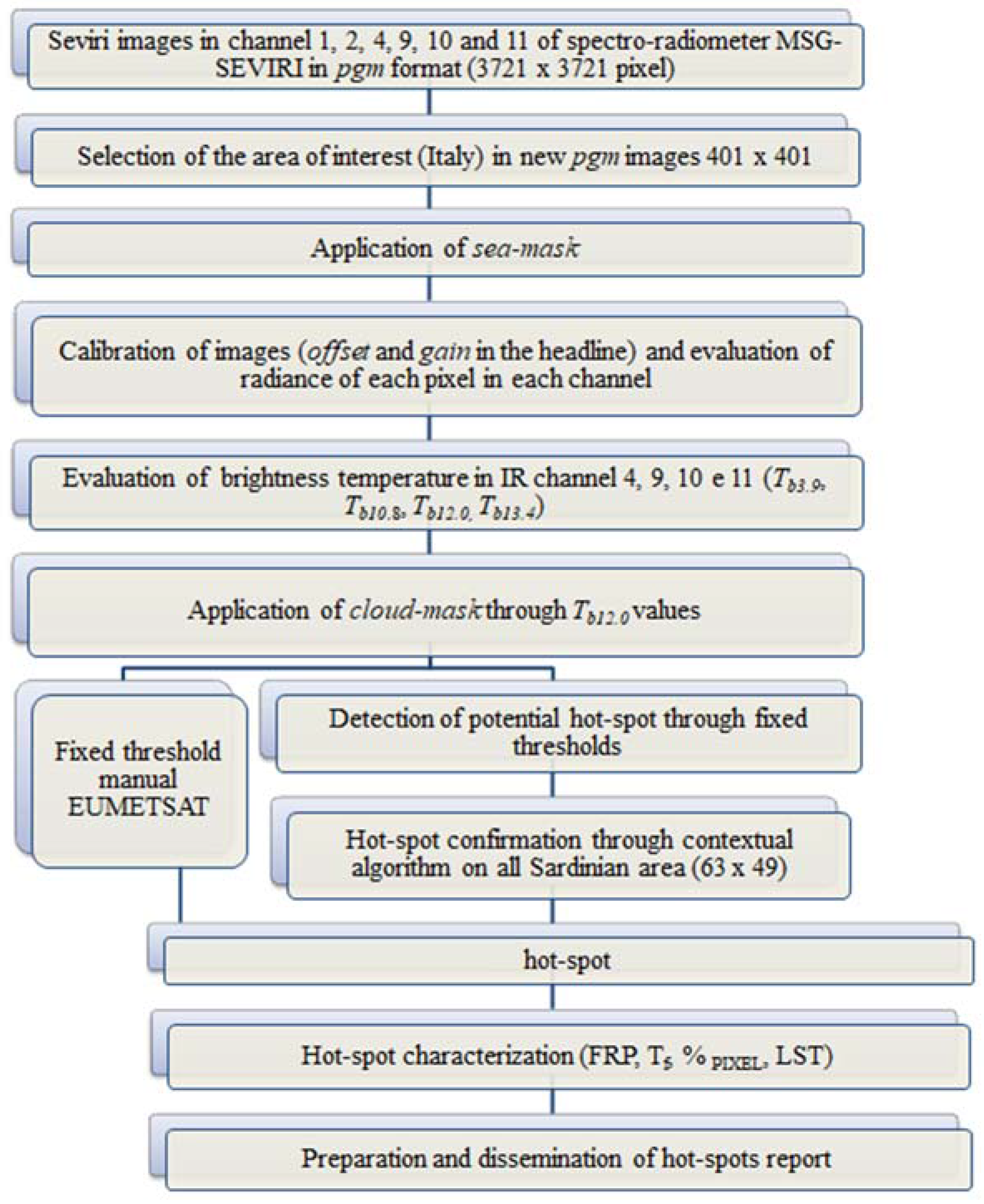
2.2.7. Nightly Hours Algorithm

For SZA < 85°, an alternative algorithm has been used due to the absence of reflected solar component. Principal differences with the daily one are:

• Cloud-mask identified using a threshold on channel 10;
• Hot-spot detection with fixed thresholds occurs with limit values of T_b3.9 and ΔT, adapted to nocturnal hours;
• Fixed values of T_b3.9 and ΔT as hot-spot detection thresholds;
• Contextual analysis carried out by using average value of T_b3.9 and ΔT on the whole of Sardinia;
• No distinction between high and low probability fire pixels.

A model of the night-time algorithm is given in Figure 6.

A pixel is considered cloudy if:

$$T_b{}_{12.0}<265\mathrm{K}$$

(39)

Fixed thresholds based on T_b3.9 and ΔT values [34] are:

$$\{\begin{array}{l}{T}_{b3.9}>290 K\\ \mathit{\Delta }T>1 K\end{array}$$

(40)

Due to the high number of omission errors detected using fixed thresholds, also for nocturnal hours a detection method based on fixed pre-thresholds and confirmation has been used.

A pixel is considered as potential hot-spot if it satisfies the following revised thresholds:

$$\{\begin{array}{l}{T}_{b3.9}>285 K\\ \mathit{\Delta }T>-2 K\end{array}$$

(41)

Hot-spot confirmation is made with contextual-analysis. A pixel is confirmed as hot-spot if it satisfies:

$$\{\begin{array}{l}{T}_{b3.9}>T_{b3.9}{}_{\_SAR}+1.5\cdot {\sigma }_{T_{b3.9}{}_{\_SAR}}\\ \mathit{\Delta }T>\mathit{\Delta }{T}_{\_SAR}+1.5\cdot {\sigma }_{\mathit{\Delta }{T}_{\_SAR}}\end{array}$$

(42)

where $T_{b3.9}{}_{\_SAR}$ and ${\sigma }_{T_{b3.9}{}_{\_SAR}}$ are average values and standard deviation of T_b3.9 for the whole of Sardinia; $\mathit{\Delta }{T}_{\_SAR}$ and ${\sigma }_{\mathit{\Delta }{T}_{\_SAR}}$ are average values of ΔT for the whole of Sardinia.

A final confirmation is given by FRP analysis. A pixel is confirmed as hot-spot only if (38) is satisfied.

3. Data Validation

Validation of SFIDE output has been made on Sardinian area using images acquired in 2014 (from 2 to 8 July and from 31 July to 6 August) and August 2016. These results have been compared with in situ data collected by CFVA (http://www.sardegnaambiente.it/corpoforestale/) and this comparison concerns fires detectable from geostationary orbit because of their dimension and coverage features. Another validation has been made by using the low orbit data of MODIS sensor (https://modis.gsfc.nasa.gov). It should be underlined that the fire season in the area of interest commonly goes from the 1 June to the 30 September.

3.1. Comparison with In Situ Measurements

Since CFVA measurements consist in total burned area evaluated at the end of the incendiary event, only fires larger- in total- than 5 ha have been considered. Instantaneous in situ measurements are not available, and minimum detectable fire size from geostationary orbit has been evaluated using [6] in 0.1–0.2 ha [35,36,37]. Fires in cloudiness and high reflectance area have been excluded from the comparison. The results (

Table 2. SFIDE omission/commission matrix.

Detected Fire Events	Omitted Fire Events	Detected Hot-Spot	False Alarms
45	4 (8.9%)	464	32 (6.9%)

) show that 41 on 45 detectable fires were detected (91.1%), with less than 9% omission error.

Furthermore, a significant result is that not only fires that developed in forest area were detected: a certain percentage of detected hot-spots corresponds to fires that occurred in mixed or grassy covered areas. Even a considerable number of fire having burned less than 5 hectares have been detected, with an amount of 45 fires detected during the validation period.

SFIDE output consists in 464 hot-spots, of which only 32 (6.9%) are commission errors (false alarms). Trigger thresholds (Equations (24) and (25) or (30) and (31)) have been able to detect 31.25% of detectable fires. The utility of the change detection based approach is confirmed by the fact that the tests of Equations (23) and (24) (or Equations (30) and (31)) allow an early detection of the fires in 100% of the cases. It is necessary to highlight that these thresholds are decisive for the triggering phases and, moreover, trigger thresholds are able to detect fires only when they are in their increasing phase, that is essential for the purpose of real time monitoring of SFIDE.

Other hot-spots has also been detected from contextual thresholds (about 73.49%) and fixed thresholds (about 62.07%).

One of the principal causes of false alarms is the sudden variation of reflectance values in channel 2, together with a sudden variation of T_b3.9 and consequently ΔT. In nocturnal hours, when these phenomena do not appear, 100% of detected hot-spots has indeed been classified as real fire. An in-depth analysis of the hot-spots classified as false alarms, shows they mainly depends by fixed threshold.

By considering the purpose of real time monitoring, the optimal solution would be to use the trigger threshold for the detection of new fires, and the fixed threshold in the following phases to continue to consider pixel as burning and continue to estimate the FRP.

The tests carried out in 2016 shows how the purpose of SFIDE is achieved also using samples of data different from the ones used for the statistical analysis (as in 2014), and how the introduction of new thresholds is necessary for the purpose of real time monitoring.

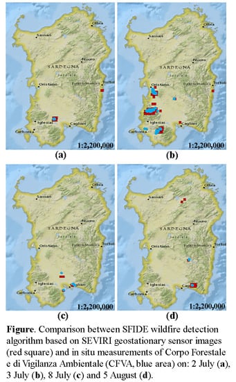
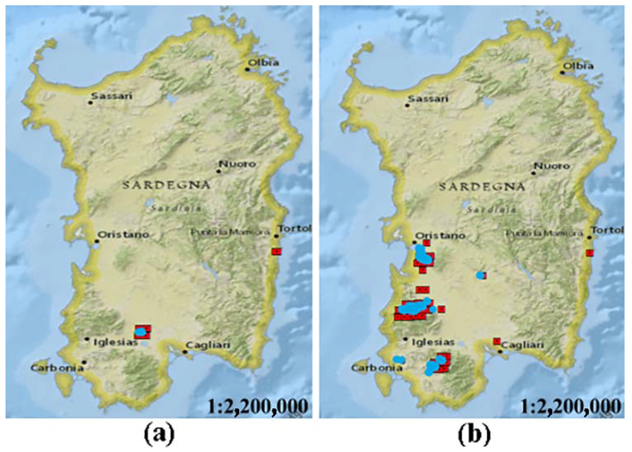
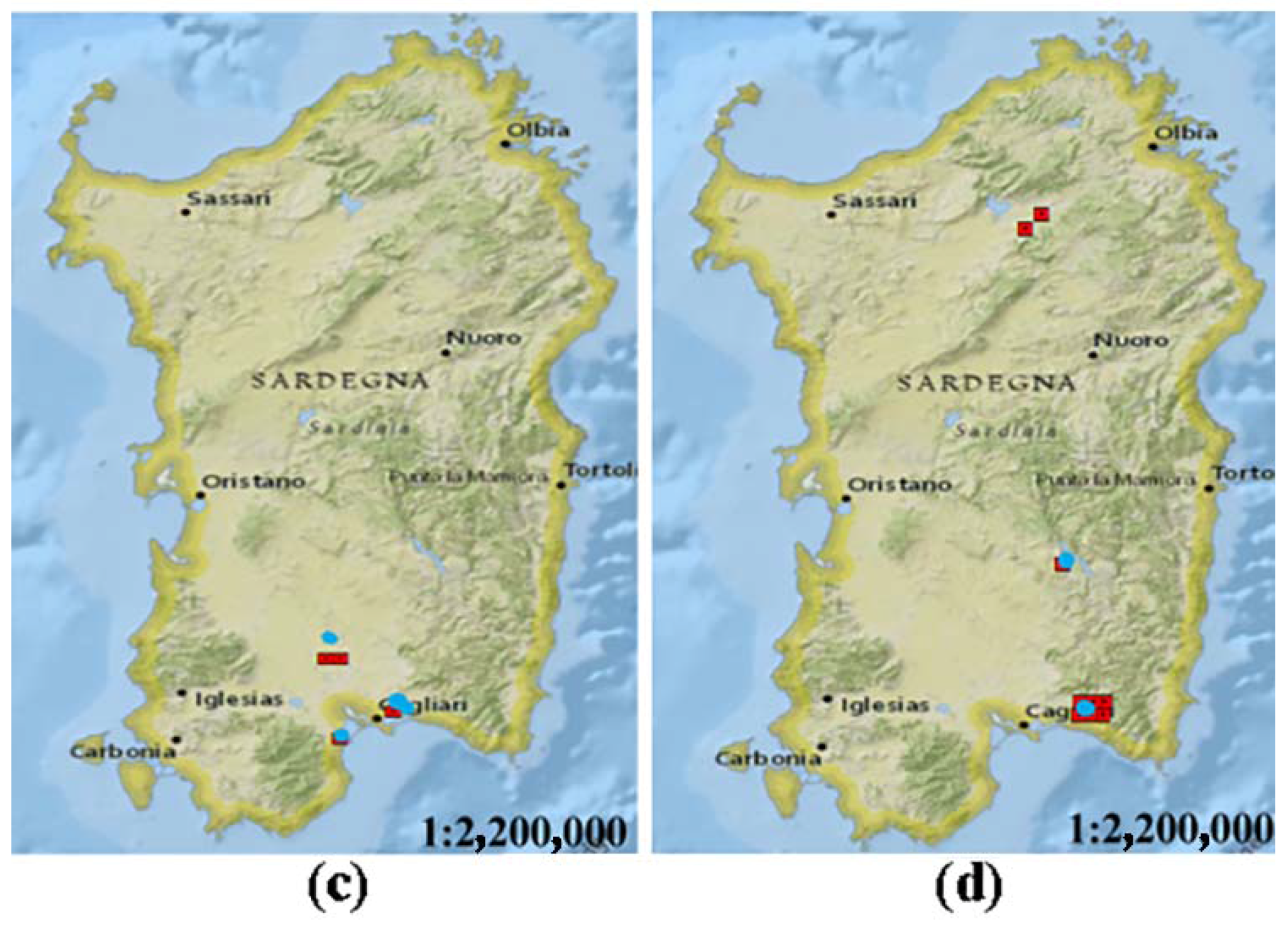
Figure 7, processed with commercial software ArcMap, shows a comparison between SFIDE detected hot-spots (red square) and in situ measurements of CFVA (blue area) on 2, 3 and 8 of July and 5 of August 2014. Figure corresponding to 3rd July (Figure 7b) shows non-detected fires due to a local high cloudiness. Red squares near in situ reported fires represent a kind of detected hot-spot due to sensor saturation issues.

3.2. Comparison with MODIS Sensor

Comparison with MODIS sensor has been conducted with images acquired in 2014 (from 2 to 8 July and from 31 July to 6 August), MODIS algorithm results over evaluated period, consist in 3 fires compared to 20 fires detected by SFIDE algorithm and 22 reported by CFVA. Only one of the fires detected by MODIS was not-detected by SFIDE due to a meteorological condition (local high cloudiness). These results show:

−

the importance of a geostationary orbit sensor that allows real time monitoring due to a high update frequency: 96 daily images by SEVIRI and 2–4 by MODIS;

−

that, particularly relevant, fires larger than 100 [ha] have not been detected by MODIS sensor, and this result confirms the major advantages of SFIDE algorithm also regarding the number of detected fires.

3.3. Fire Monitoring Examples

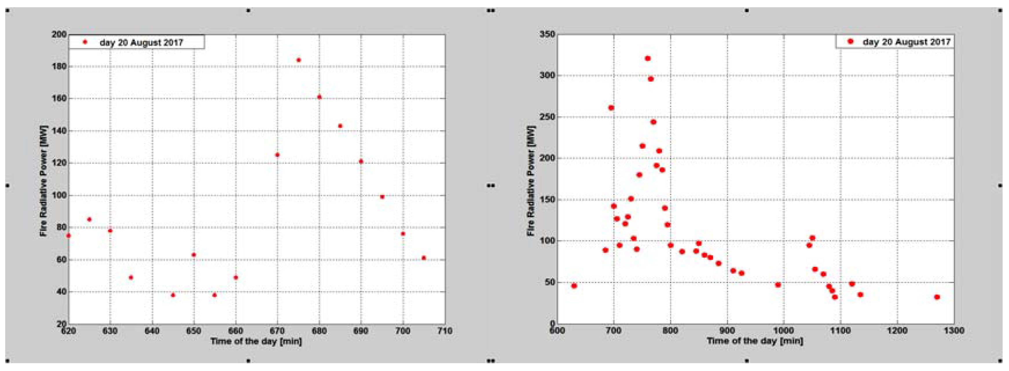
Using the high refresh frequency of the SEVIRI images, in particular in the case of MSG 9 also known as RSS (Rapid Scanning Service) characterized by a refresh frequency of 5 min, it is, in general, possible to follow in a quasi-continuous way the evolution of the fire. This allows, possibly, the deduction of interesting information on the fire behavior and the effectiveness of the fire-fighting activity. Figure 8 allows one to explain this point better. The figure compares, through the FRP (measured in MW), the behavior of two fires that occurred in the Calabria region on 20 August 2017. The behavior of one of the two fires (the one for which the FRP is shown on the left plot) seems much more ‘natural’ or regular than the other. Further, this fire lasts also much less than the other, about 1.5 h (90 min) instead of 11 h (660 min). It is also less intense reaching a maximum FRP of 180 MW instead of 330 MW, as in the case of the other fire. This suggests that fire corresponding to left plot of Figure 8 extinguished itself for natural reasons not for the intervention of firefighters.

4. Conclusions

The SFIDE algorithm was developed by authors several years ago [22] in the framework of a project funded by the Italian Space Agency devoted to implement a forest fires early detection and monitoring system based on satellite images coming from the geostationary sensor SEVIRI on board of the MSG satellites series. This paper presents a new version of the algorithm aiming, in particular, at reducing the false alarm rate. This updated version of the algorithm takes into account other previously developed methods for fire detection in order to:

−

Improve the estimate of the reference temperature used to define a pixel as interested by a fire;

−

Improve the cloud mask accuracy thus reducing the risk of false alarms;

−

Exploit better the high refresh rate of the images to implement several tests for accurate detection of forest fires.

The results of the comparison of the events detected in Sardinia by the algorithm with those provided by local authorities and/or detected by other higher resolution satellite sensor (MODIS) confirm the improvement made. In fact, in the present version the algorithm provides an omission error of less than 9% and a commission error of less than 7%. At this point a further step is needed, which is, to reduce the approximation in the localization of the fire (the fire can occupy any position in the pixel of 4 × 4 km²). At present, the position of the fire corresponds to the coordinates of the center of the pixel. Possibly exploiting the simultaneous observation from 2 geostationary satellites like MSG 8 (RSS) and MSG 9 (IODC) and introducing a fuel map of the area of interest a more accurate localization of the fire position could be achieved. This will possibly be discussed in a future paper.

References

- Schmuck, G.; San-Miguel-Ayanz, J.; Camia, A.; Durrant, T.; Santos De Oliveira, S.; Boca, R.; Whitmore, C.; Giovando, C.; Libertà, G.; Corti, P.; et al. Forest Fires in Europe; Publications Office of the European Union: Luxembourg, 2010. [Google Scholar]
- Laneve, G.; Fusilli, L.; Marzialetti, P.; De Bonis, R.; Bernini, G.; Tampellini, L. Development and Validation of Fire Damage-Severity Indices in the Framework of the PREFER Project. IEEE J. Sel. Top. Appl. Earth Obs. Remote Sens. 2016, 9, 2806–2817. [Google Scholar] [CrossRef]
- Ager, A.A.; Preisler, H.K.; Arca, B.; Spano, D.; Salis, M. Wildfire risk estimation in the Mediterranean area. Environmetrics 2009, 25, 384–396. [Google Scholar] [CrossRef]
- Sifakis, N.I.; Iossifidis, C.; Kontoes, C.; Keramitsoglou, I. Wildfire Detection and Tracking over Greece Using MSG-SEVIRI Satellite Data. Remote Sens. 2011, 3, 524–538. [Google Scholar] [CrossRef]
- Martín, M.P.; Ceccato, P.; Flasse, S.; Downey, I. Fire detection and fire growth monitoring using satellite data. In Remote Sensing of Large Wildfires; Springer: Berlin/Heidelberg, Germany, 1999; pp. 101–122. [Google Scholar]
- Dozier, J. A method for satellite identification of surface temperature fields of subpixel resolution. Remote Sens. Environ. 1981, 11, 221–229. [Google Scholar] [CrossRef]
- Salomonson, V.V.; Barnes, W.L.; Maymon, P.W.; Montgomery, H.E.; Ostrow, H. MODIS: Advanced facility instrument for studies of the earth as a system. IEEE Trans. Geosci. Remote Sens. 1989, 27, 145–153. [Google Scholar] [CrossRef]
- Kaufman, Y.J.; Justice, C.O.; Flynn, L.P.; Kendall, J.D.; Prins, E.M.; Giglio, L.; Ward, D.E.; Menzel, W.P.; Setzer, A.W. Potential global fire monitoring from EOS-MODIS. J. Geophys. Res. Atmos. 1998, 103, 32215–32238. [Google Scholar] [CrossRef]
- Justice, C.O.; Giglio, L.; Korontzi, S.; Owens, J.; Morisette, J.T.; Roy, D.; Descloitres, J.; Alleaume, S.; Petitcolin, F.; Kaufman, Y. The MODIS fire products. Remote Sens. Environ. 2002, 83, 244–262. [Google Scholar] [CrossRef]
- Giglio, L.; Descloitres, J.; Justice, C.O.; Kaufman, Y.J. An enhanced contextual fire detection algorithm for MODIS. Remote Sens. Environ. 2003, 87, 273–282. [Google Scholar] [CrossRef]
- Giglio, L.; Csiszar, I.; Restas, A.; Morisette, J.T.; Schroeder, W.; Morton, D.; Justice, C.O. Active fire detection and characterization with the advanced spaceborne thermal emission and reflection radiometer (ASTER). Remote Sens. Environ. 2008, 112, 3055–3063. [Google Scholar] [CrossRef]
- Giglio, L.; Schroeder, W.; Justice, C.O. The collection 6 MODIS active fire detection algorithm and fire products. Remote Sens. Environ. 2016, 178, 31–41. [Google Scholar] [CrossRef]
- Robinson, J.M. Fire from space: Global fire evaluation using infrared remote sensing. Int. J. Remote Sens. 1991, 12, 3–24. [Google Scholar] [CrossRef]
- Flasse, S.P.; Ceccato, P. A contextual algorithm for AVHRR fire detection. Int. J. Remote Sens. 1996, 17, 419–424. [Google Scholar] [CrossRef]
- Giglio, L.; Kendall, J.D.; Justice, C.O. Evaluation of global fire detection algorithms using simulated AVHRR infrared data. Int. J. Remote Sens. 1999, 20, 1947–1985. [Google Scholar] [CrossRef]
- Schroeder, W.; Oliva, P.; Giglio, L.; Csiszar, I.A. The new VIIRS 375 m active fire detection data product: Algorithm description and initial assessment. Remote Sens. Environ. 2014, 143, 85–96. [Google Scholar] [CrossRef]
- Prins, E.M.; Feltz, J.M.; Menzel, W.P.; Ward, D.E. An overview of GOES-8 diurnal fire and smoke results for SCAR-B and 1995 fire season in South America. J. Geophys. Res. Atmos. 1998, 103, 31821–31835. [Google Scholar] [CrossRef]
- Reid, J.S.; Koppmann, R.; Eck, T.F.; Eleuterio, D.P. A review of biomass burning emissions part II: Intensive physical properties of biomass burning particles. Atmos. Chem. Phys. 2005, 5, 799–825. [Google Scholar] [CrossRef]
- Xu, W.; Wooster, M.J.; Roberts, G.; Freeborn, P. New GOES imager algorithms for cloud and active fire detection and fire radiative power assessment across North South and Central America. Remote Sens. Environ. 2010, 114, 1876–1895. [Google Scholar] [CrossRef]
- Aminou, D.M.A. MSG’s SEVIRI instrument. ESA Bull. 2002, 111, 15–17. [Google Scholar]
- Calle, A.; Casanova, J.L.; Romo, A. Fire detection and monitoring using MSG Spinning Enhanced Visible and Infrared Imager (SEVIRI) data. J. Geophys. Res. Biogeosci. 2006, 111, G04S06. [Google Scholar] [CrossRef]
- Laneve, G.; Castronuovo, M.M.; Cadau, E.G. Continuous monitoring of forest fires in the Mediterranean area using MSG. IEEE Trans. Geosci. Remote Sens. 2006, 44, 2761–2768. [Google Scholar] [CrossRef]
- Roberts, G.J.; Wooster, M.J. Fire detection and fire characterization over Africa using Meteosat SEVIRI. IEEE Trans. Geosci. Remote Sens. 2008, 46, 1200–1218. [Google Scholar] [CrossRef]
- Amraoui, M.; DaCamara, C.C.; Pereira, J.M.C. Detection and monitoring of African vegetation fires using MSG-SEVIRI imagery. Remote Sens. Environ. 2010, 114, 1038–1052. [Google Scholar] [CrossRef]
- Laneve, G.; Jahjah, M.; Ferrucci, F.; Battazza, F. SIGRI project: The development of the fire vulnerability index. In Proceedings of the 34th International Symposium on Remote Sensing of Environment, Sydney, Australia, 10–15 April 2011. [Google Scholar]
- Laneve, G.; Cadau, E.; Ferrucci, F.; Rongo, R.; Guarino, A.; Fortunato, G.; Loizzo, R. SIGRI-an Integrated System for Detecting, Monitoring, Characterizing Forest Fires and Assessing damage by LEO-GEO Data. Ital. J. Remote Sens. 2012, 44, 19–25. [Google Scholar] [CrossRef]
- Laneve, G.; Jahjah, M.; Ferrucci, F.; Hirn, B.; Battazza, F.; Fusilli, L.; De Bonis, R. SIGRI project: Products validation results. IEEE J. Sel. Top. Appl. Earth Obs. Remote Sens. 2014, 7, 895–905. [Google Scholar] [CrossRef]
- Schmid, J. The SEVIRI instrument. In Proceedings of the 2000 EUMETSAT Meteorological Satellite Data User’s Conference, Bologna, Italy, 29 May–2 June 2000; Volume 29. [Google Scholar]
- Saunders, R.W.; Kriebel, K.T. An improved method for detecting clear sky and cloudy radiances from AVHRR data. Int. J. Remote Sens. 1988, 9, 123–150. [Google Scholar] [CrossRef]
- Zhukov, B.; Lorenz, E.; Oertel, D.; Wooster, M.; Roberts, G. Spaceborne detection and characterization of fires during the bi-spectral infrared detection (BIRD) experimental small satellite mission (2001–2004). Remote Sens. Environ. 2006, 100, 29–51. [Google Scholar] [CrossRef]
- Wooster, M.J.; Roberts, G.; Perry, G.L.W.; Kaufman, Y.J. Retrieval of biomass combustion rates and totals from fire radiative power observations: FRP derivation and calibration relationships between biomass consumption and fire radiative energy release. J. Geophys. Res. Atmos. 2005, 110. [Google Scholar] [CrossRef]
- Kaiser, J.W.; Heil, A.; Andreae, M.O.; Benedetti, A.; Chubarova, N.; Jones, L.; Morcrette, J.J.; Razinger, M.; Schultz, M.G.; Suttie, M.; et al. Biomass burning emissions estimated with a global fire assimilation system based on observed fire radiative power. Biogeosciences 2012, 9, 527–554. [Google Scholar] [CrossRef] [Green Version]
- Sobrino, J.A.; Romaguera, M. Land surface temperature retrieval from MSG1-SEVIRI data. Remote Sens. Environ. 2004, 92, 247–254. [Google Scholar] [CrossRef]
- Joro, S.; Samain, O.; Yildirim, A.; Van De Berg, L.; Lutz, H.J. Towards an Improved Active Fire Monitoring Product for MSG Satellites. EUMETSAT. 2008. Available online: http://citeseerx.ist.psu.edu/viewdoc/download?doi=10.1.1.611.1456&rep=rep1&type=pdf (accessed on 9 May 2018).
- Giglio, L.; Schroeder, W. A global feasibility assessment of the bi-spectral fire temperature and area retrieval using MODIS data. Remote Sens. Environ. 2014, 152, 166–173. [Google Scholar] [CrossRef]
- Wooster, M.J.; Roberts, G.; Perry, G.L.W.; Kaufman, Y.J. Retrieval of biomass combustion rates and totals from fire radiative power observations: Application to southern Africa using geostationary SEVIRI imagery. J. Geophys. Res. 2005, 110, D21111. [Google Scholar]
- Laneve, G.; Castronuovo, M.; Cadau, E. Assessment of the fire detection limit using SEVIRI/MSG sensor. In Proceedings of the IGARSS, Denver, CO, USA, 31 July–4 August 2006; pp. 4157–4160. [Google Scholar]
Figure 1.
Averaged annual burned area in the European countries most affected by fires between 1980 and 2013, compared with more recent years [2].