Article

Identifying Flood Events over the Poyang Lake Basin Using Multiple Satellite Remote Sensing Observations, Hydrological Models and In Situ Data

1
MOE Key Laboratory of Fundamental Physical Quantities Measurement, Hubei Key Laboratory of Gravitation and Quantum Physics, Institute of Geophysics, School of Physics, Huazhong University of Science and Technology, Wuhan 430074, China
2
State Key Laboratory of Geodesy and Earth’s Dynamics, Institute of Geodesy and Geophysics, Chinese Academy of Sciences, Wuhan 430077, China
3
Collaborative Innovation Center of Geospatial Technology, Wuhan University, Wuhan 430079, China
4
School of Engineering, University of Newcastle, Callaghan 2308, New South Wales, Australia
5
School of Resource and Environmental Science, Wuhan University, Wuhan 430079, China
6
Key Laboratory of Earthquake Geodesy, Institute of Seismology, China Earthquake Administration, Wuhan 430071, China
*
Authors to whom correspondence should be addressed.
Remote Sens. 2018, 10(5), 713; https://doi.org/10.3390/rs10050713
Submission received: 15 March 2018 / Revised: 25 April 2018 / Accepted: 4 May 2018 / Published: 5 May 2018
(This article belongs to the Special Issue GRACE Facing the Challenge of Extreme Spatial and Temporal Scales)

Abstract

:
The Poyang Lake, the largest freshwater lake in China, is famous for its ecological and economic importance as well as frequent flood characteristics. In this study, multiple satellite remote sensing observations (e.g., GRACE, MODIS, Altimetry, and TRMM), hydrological models, and in situ data are used to characterize the flood phenomena over the Poyang Lake basin between 2003 and 2016. To improve the accuracy of the terrestrial water storage (TWS) estimates over the Poyang Lake basin, a modified forward-modeling method is introduced in the GRACE processing. The method is evaluated using the contaminated noise onboard observations for the first time. The results in both spectral and spatial domains infer a good performance of the method on the suppression of high-frequency noise while reducing the signal loss. After applying forward-modeling method, the TWS derived from the GRACE spherical harmonic coefficients presents a comparable performance with the solution derived from the newly released CSR Release05 mascon product over the Poyang Lake basin. The flood events in 2010 and 2016 are identified from the positive anomalies in non-seasonal TWSs derived by GRACE and hydrological models. The flood signatures also coincide with the largest inundated areas estimated from MODIS data, and the observed areas in 2010 and 2016 are 3370.3 km2 (30% higher than the long-term mean) and 3445.0 km2 (33% higher), respectively. The water levels in the Hukou station exceed the warning water level for 25 days in 2010 and 28 days in 2016. These continuous warning-exceeded water levels also imply the severe flood events, which are primarily driven by the local plenteous precipitation in the rainy season (1528 mm in 2010, 1522 mm in 2016).

Graphical Abstract

1. Introduction

The Poyang Lake, the largest freshwater lake in China, is famous for its great ecological, economic and cultural importance. Due to the dramatic variation of regional climate, the Poyang Lake basin becomes one of the most frequently flooded areas in China, inflicting enormous losses in human casualties, wildlife, and productions [1,2,3,4]. Aiming to minimize the hazards on natural and economical activities, the characteristics of historical flood events need to be analyzed in detail. For this reason, this study uses the remote sensing observations and in situ data to assess the water storage variations as well as to identify the flood occurrences over the Poyang Lake basin.
Multiple remote sensing observations have been used to identify the flood events over the Poyang Lake [5,6,7,8]. Among these, the Moderate Resolution Imaging Spectroradiometer (MODIS) [9] can quantify the variation of the inundated area [5,10,11]; the altimetry satellites can detect the water level variations of the lake [12]; and the Tropical Rainfall Measuring Mission (TRMM) [13] can monitor the temporal variations of precipitation. However, these missions are not able to detect the total terrestrial water storage (TWS) variations, which is crucial for the analysis of the extreme hydrological activities [14,15,16,17,18]. To address this issue, the data collected by the Gravity Recovery And Climate Experiment (GRACE) satellite mission is used in our study [19]. In contrast to the terrestrial surface reflectance observations, GRACE senses the TWS variations in all components (e.g., snow water, surface water, soil moisture, and groundwater). To date, this study analyzes for the first time the flood events over the Poyang Lake basin using GRACE, MODIS, TRMM, and altimetry satellite observations simultaneously.
While GRACE data is very important to monitor TWS variations, the effective approach of suppressing its high-frequency errors (presented as north-south stripes in the spatial domain) is one of the major challenges. Some special designed spatial filters are commonly used to suppress these errors. For example, the Gaussian smoothing filter is designed to alleviate the high-frequency noise [20], while the de-stripping filter is used to reduce the correlated noise [21]. However, the application of filters commonly leads to leakage errors [22,23,24,25]. The forward-modeling method can be employed to reduce leakage errors [26,27,28,29]. The method is independent of external data, e.g., a hydrology model. Its main idea is to iteratively retrieve the leakage signal from ocean to land. However, this method has been only validated by an error-free synthetic data for Amundsen Sea Embayment [30]. Therefore, in the first instance, a closed-loop study is made to validate the forward-modeling method in the noise contaminated condition. During the validation, the GRACE onboard observations errors and various prior force model errors are also considered. After method validation, the TWS variations of Poyang Lake basin are calculated with the Release05 temporal gravity field model from the Center Space Research (CSR) [31]. As will be shown later, the results present comparable performance with the newly released CSR Release05 mascon product [32] and other external data, which also indicates the good performance of the forward-modeling method.
For a better understanding of the flood properties over the Poyang Lake basin, apart from remote sensing data, various in situ datasets and three hydrological models are also used. Two hydrological models are used to estimate the soil moisture variations: (1) the Noah land surface model of Global Land Data Assimilation System (GLDAS) [33]; and (2) the ERA-Interim reanalysis dataset from the European Centre for Medium-Range Weather Forecasts (ECMWF) [34]. The other hydrological model PCRaster Global Water Balance (PCR-GLOBWB) [35,36], which contains soil moisture but also surface water and groundwater, is compared with GLDAS and ERA-Interim to distinguish the contribution of other water storage components. In addition, various in situ datasets (including water level, temperature, precipitation, and evaporation) are also used to analyze the hydrological activities over the Poyang Lake basin.
The objectives of this study are (1) to validate the forward-modeling method using noise contaminated observations of the GRACE-type mission, and (2) to identify the flood events over the Poyang Lake basin between 2003 and 2016 using multiple remote sensing observations, hydrological models and in situ data.

2. Study Region and Datasets
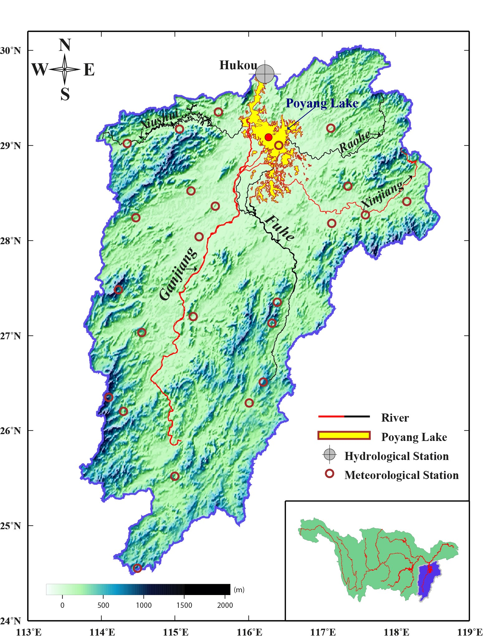
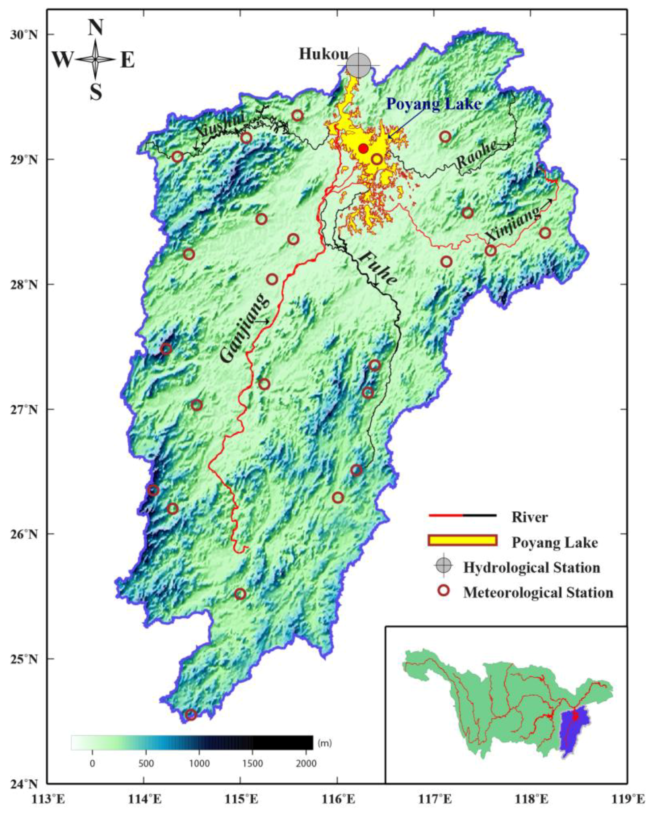
2.1. Study Region

The total drainage area of the Poyang Lake basin (see Figure 1) is about 1.622 × 10⁵ km2, accounting for about 9% of the total drainage area of the Yangtze River basin. The region is characterized by significant precipitation variations, resulting in a rainy season from March to August and a dry season from September to February. Poyang Lake, located in the north of our study region, is the major natural reservoir of the Yangtze River (see the inset map in Figure 1). The lake discharges into the Yangtze River through Hukou hydrological station and receives water from Raohe, Xinjiang, Fuhe, Ganjiang, and Xiushui. Due to the seasonal precipitation, the inundated area of Poyang Lake reaches to > 3000 km2 in the rainy season and shrinks to < 1000 km2 in the dry season.

2.2. Datasets

2.2.1. GRACE Data

The CSR Release05 monthly gravity field data [37] (at degree and order 60) were used to estimate the TWS variations over the Poyang Lake basin. The period of the products spanned from January 2003 to March 2016. Because of the poor quality of GRACE observations in June 2003, the corresponding model was unavailable. In addition, the numerous outages of GRACE payloads (especially accelerometers) leaded to the absence of other 17 monthly gravity field models after 2010 [38]. The cubic spline interpolation was used to fill the missing TWS values in these months.
The CSR Release05 models in the form of spherical harmonic coefficients (SHCs) were processed as follows: (1) the degree 1 coefficients provided by Swenson et al. [39] were restored; (2) the degree 2 order 0 (C20) coefficients were replaced by the satellite laser ranging measurements [40]; (3) the long-term-mean was removed from the monthly product to obtain the variation of SHCs; (4) the de-correlation filter associated with a polynomial of order 3 and harmonic order 6 and higher (P3M6) was used to reduce the correlated errors in GRACE data [21]; and (5) the Gaussian filter with a radius of 300 km was used to suppress the high frequency noise [20]. After processing SHCs, the TWS variations were computed following Wahr et al. [41]. The forward-modeling method was then applied to alleviate leakage errors. More details about forward-modeling method are discussed in Section 3.1.
In addition, the CSR monthly mass grid product associated with scale factors [31] and CSR Release05 mascon products [32] were used for comparison. The mass grid products were obtained from GRACE Tellus (https://grace.jpl.nasa.gov/data/), and the mascon products were downloaded from the CSR data archive (http://www2.csr.utexas.edu/grace/). The scale factors of GRACE Tellus grid products were computed based on the land surface model (NCAR’s CLM4). In the Poyang Lake basin, the mean value of the scale factor is 1.53. The long-term mean and linear trends of the TWSs time series were removed to reduce the contribution of the decadal and long-term variation of the land hydrology signal [1].

2.2.2. Hydrological Models
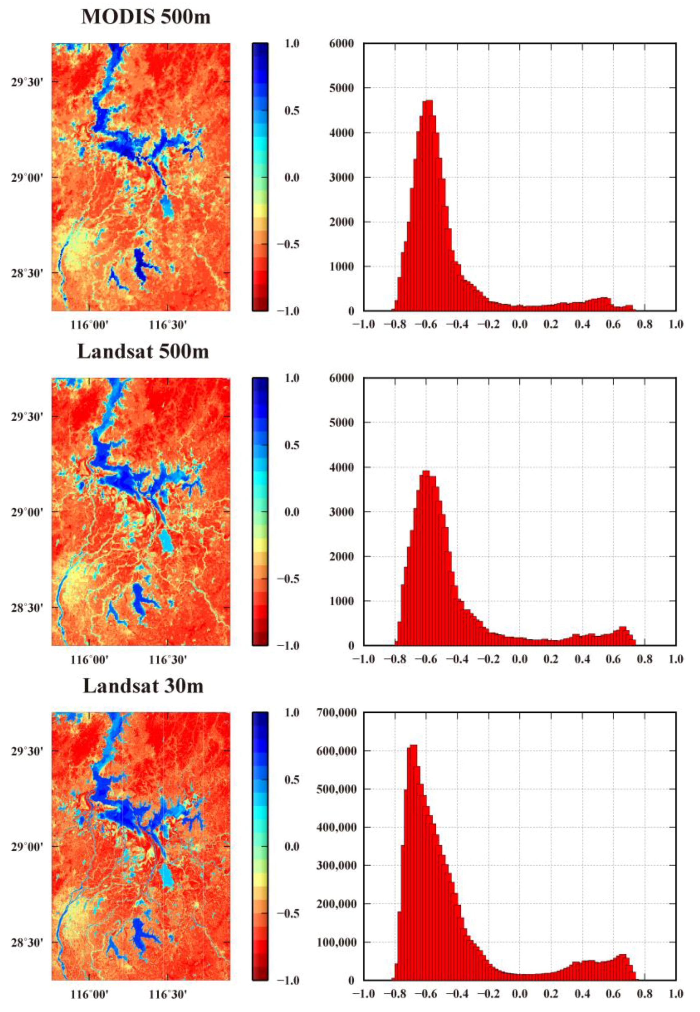
Three hydrological models were used to estimate the water storage variations in different components: (1) The 1-degree monthly GLDAS-Noah model was used in this study. As the canopy water and snow water storage accounts for less than 1% in the Poyang Lake basin, the TWS was computed only as the sum of four soil moisture layers: 0~10, 10~40, 40~100 and 100~200 cm [33]. (2) The monthly ERA-Interim model was used for comparison. The TWS was computed as the sum of four soil moisture layers: 0~7, 7~28, 28~100 and 100~255 cm [34]. (3) The PCR-GLOBWB model was used to simulate the water storage variations, consisting of the surface, two soil layers (0~30 and 30~150 cm), and groundwater [35,36]. In contrast to GLDAS and ERA-Interim models, complete water storage was likely observed in PCR-GLOBWB regarding the inclusion of the groundwater component. The PCR-GLOBWB model was anticipated to be more efficient for characterizing the hydrological events. Similar to GRACE TWS, the long-term mean and linear trends of TWS derived from three hydrological models were also removed.

2.2.3. MODIS Data

The MODIS 8-day surface reflectance product from Aqua satellite (MYD09A1) was used to estimate the inundated area variations over the Poyang Lake [9]. The spatial resolution of the product is 500 m. Based on the location of the Poyang Lake, the MODIS tile h28v06 was selected. The surface reflectance quality control flags data, as well as the cloud mask based on a threshold of the surface reflectance in the blue band ( ρ b l u e 0.2 ), were used to exclude pixels with cloud cover. In addition, the fill values and the data out of valid range were excluded. The 8-day normalized difference water index (NDWI) was then computed as [42]
N D W I = ρ g ρ N I R ρ g + ρ N I R
where ρ g and ρ N I R is the reflectance in green and near-infrared portions of the electromagnetic spectrum, respectively. The NDWI values range from -1 to 1. The pixels with positive NDWI values, representing the open water, were used to estimate the inundated area over the Poyang Lake.

2.2.4. Altimetry Data

The water levels of inland water bodies were obtained from the Database for Hydrological Time Series of Inland Waters (DAHITI) of Technische Universität München (TUM) [12]. The data were computed based on the Kalman filter approach, incorporating cross-calibrated multi-mission altimeter data from Envisat, ERS-2, Jason-1, Jason-2, TOPEX/Poseidon, and SARAL/AltiKa. The water levels of the Poyang Lake (116.27° E, 29.09° N, see Figure 1) from January 2003 to November 2015 were downloaded from http://dahiti.dgfi.tum.de/en/. As only Envisat and SARAL/AltiKa were used for the estimation of water level, there was a data gap between September 2010 and March 2013.

2.2.5. TRMM data

TRMM is a jointly mission between the Japan Aerospace Exploration Agency and NASA. It gathers the precipitation data at the region of 50°S~50°N and 180°W~180°E. The latest 3B43 Version 7 monthly data from January 2003 to December 2016 was used in this study. Note that the Version 7 TRMM dataset is a multi-satellite precipitation product [43].

2.2.6. In Situ Data

In situ data from 24 metrological stations in the Poyang Lake basin (see Figure 1) were used in this study. The metrological datasets were obtained from the Climatic Data Center of China Meteorological Administration (http://www.cma.gov.cn/2011qxfw/2011qsjgx/). Here, the monthly observations (including precipitation, evaporation and temperature) were used, and the time span was from January 2003 to December 2016. In addition, the water levels recorded by Hukou hydrological station (see Figure 1) were also used. Due to the policy of the hydrological stations, the water level data was only available for the period January 2003 to December 2013. Here, we obtained the discontinuous daily water level information from the bulletin published by the Changjiang Water Resources Commission of the Ministry of Water Resource (http://www.cjh.com.cn/pages/2016-08-01/227_188212.html), and the discontinuous monthly bulletin from the website of Jiujiang Hydrological Bureau (http://jjsw.jjrfw.com/artlist_detail.php?lbid=1133& wzid=3013). Fortunately, these bulletins provide the water levels of Hukou during the flood period from 2014 to 2016.

3. GRACE Data Processing

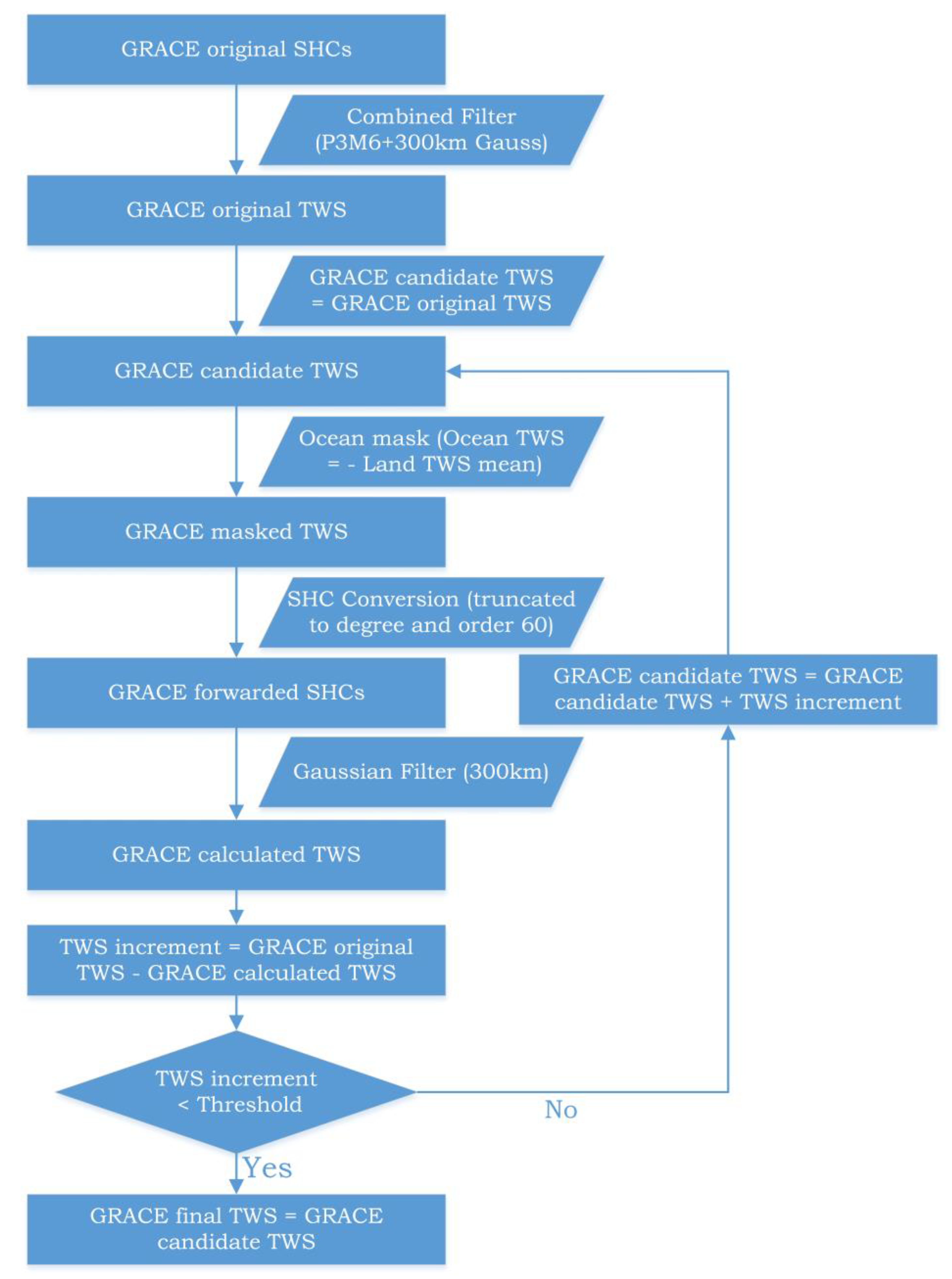
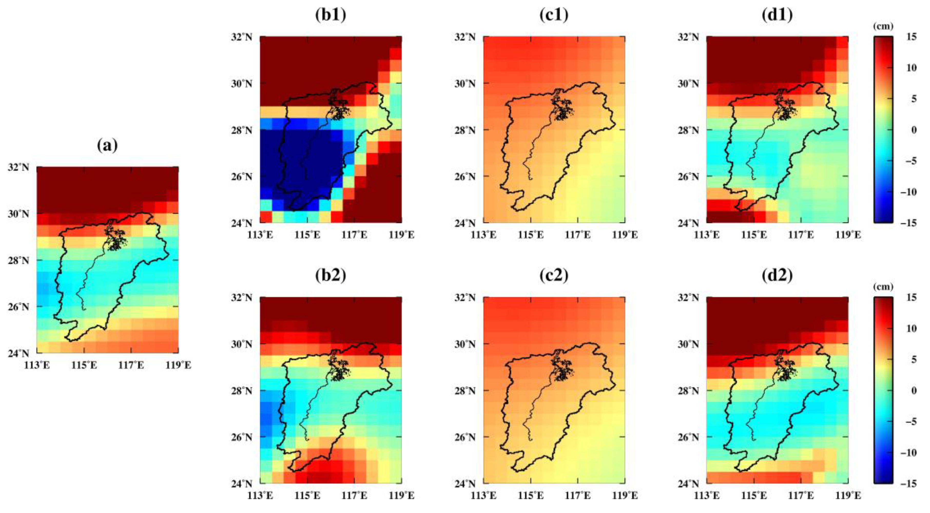
3.1. Forward-Modeling Method

The forward-modeling method is used to mitigate the GRACE leakage errors, and the method is implemented as follows (Figure 2).
(1)
Combined filter: As mentioned in Section 2.2.1, using the combined filter, the “GRACE original TWS” is derived from the GRACE original SHCs. The result is then set as the “GRACE candidate TWS”.
(2)
Ocean mask: Assuming the mass of the Earth surface is conserved, the Ocean TWS is set to the negative of the mean TWS over land. It should be noted that the land TWSs are weighted by the cosine of latitude. After applying ocean mask, the new TWS is named as “GRACE masked TWS”.
(3)
SHC conversion: The ”GRACE masked TWS” is then converted into SHCs within limited degrees and orders. Here, the truncated degree and order is set as 60. The new SHCs are called “GRACE forwarded SHCs”.
(4)
Gaussian filter: After applying Gaussian filter to “GRACE forwarded SHCs”, the “GRACE calculated TWS” is computed following Wahr et al. [41].
(5)
New iteration: TWS increment is equal to the difference between “GRACE original TWS” (in step 1) and “GRACE calculated TWS” (in step 4). The iteration is stopped when the TWS increments in the study region are all smaller than a pre-defined threshold. Otherwise a new iteration is performed. During the new iteration, the “GRACE candidate TWS” is updated as the sum of “GRACE candidate TWS” and “TWS increment”.
In this study, the iteration stops when the TWS increments in Poyang Lake basin are all smaller than 0.2 cm, or the iteration number exceeds 100. As recommended by [26,27], an acceleration factor (typically ∼1.2) is applied to “TWS increment” to increase the convergence rate. In the Poyang Lake basin, the iteration number for each monthly GRACE model is about 40~50.

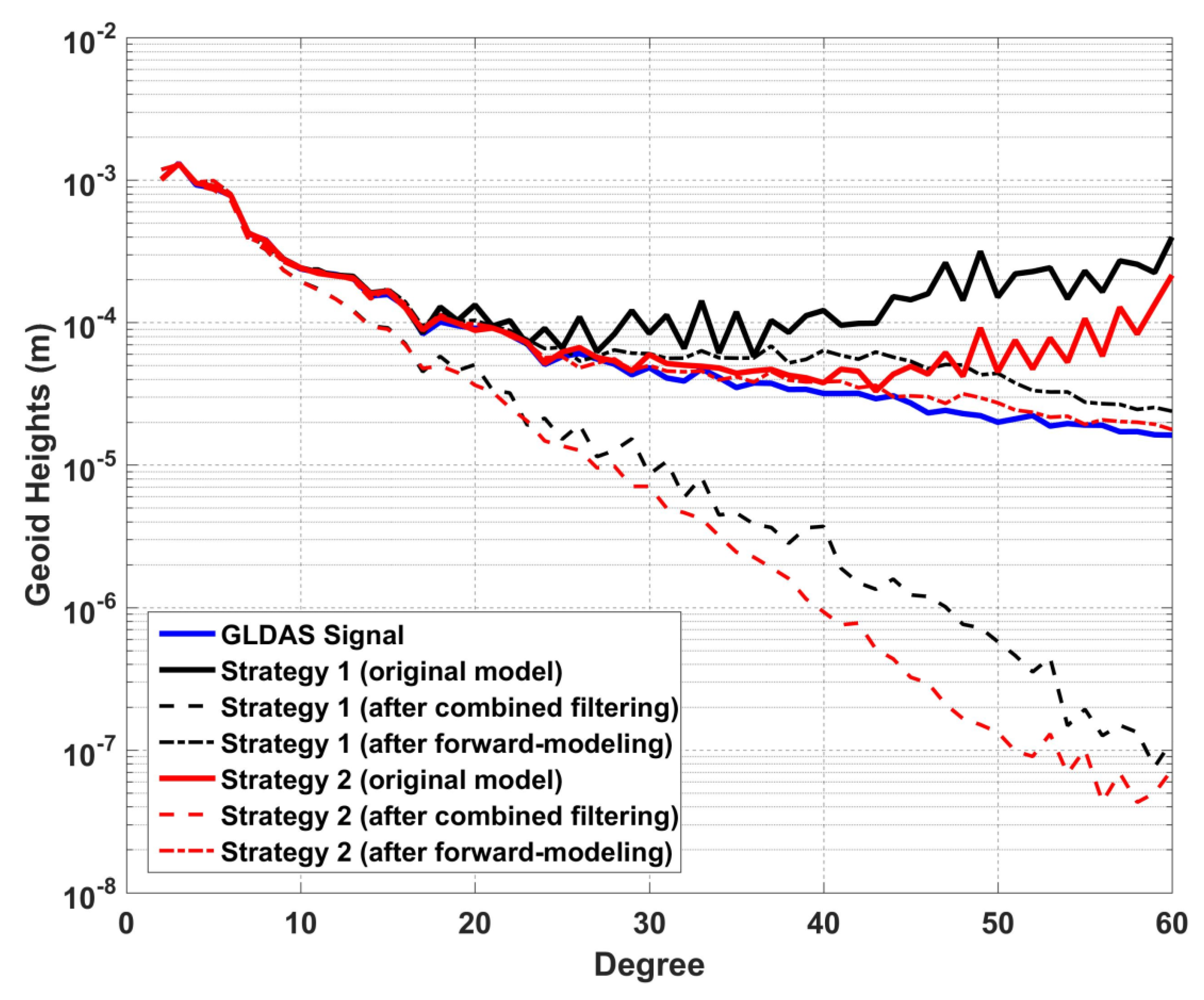
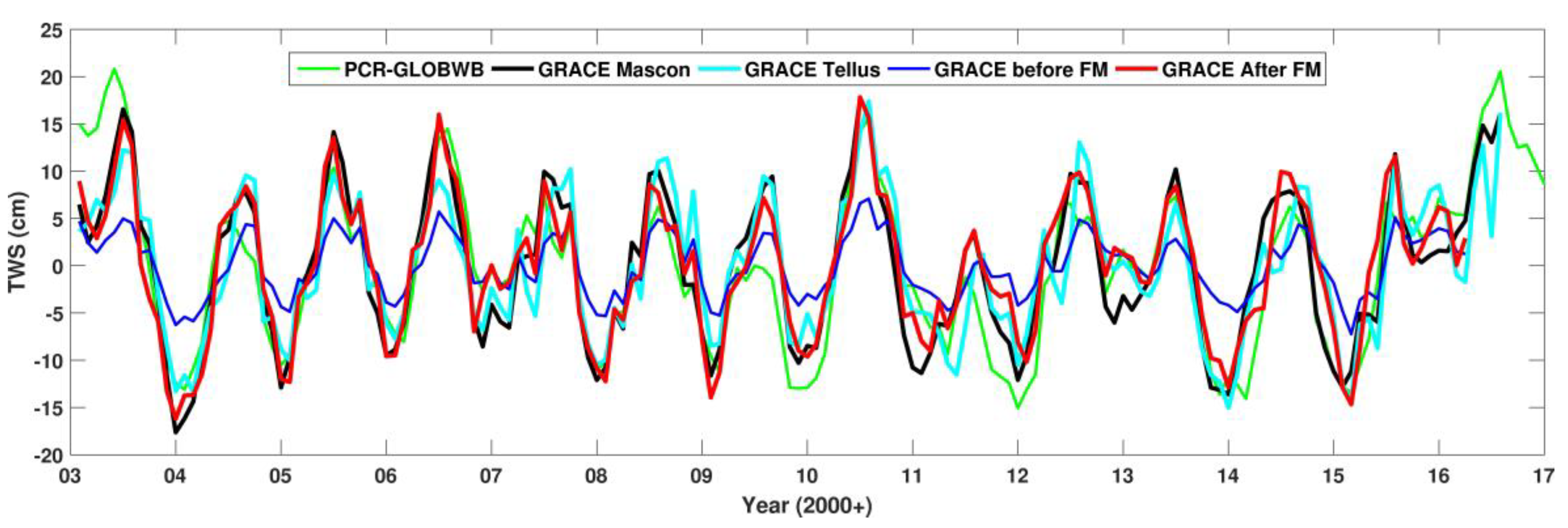
3.2. Validation of Forward-Modeling Method

To validate the forward-modeling method in noise-contaminated condition, a simulation study is implemented in this section. The noise-contaminated observations of GRACE-type mission are firstly simulated, and they are then used to determine a temporal gravity field model via a least-square adjustment method.
The simulation should mimic the real-world conditions as realistically as possible. To do this in a proper way, various background model errors (including static gravity field model, ocean tide model, and non-tidal model) as well as measurement errors (orbit and range rate) are taken into consideration (see Table 1). To evaluate the forward-modeling method in different noise scenes, the white noise in range rate of 2.5 × 10⁻⁷ m/s is introduced for the current GRACE-type mission in Strategy 1 [44], while 5.0 × 10⁻⁸ m/s range rate noise is added for the future GRACE-type mission (e.g., GRACE Follow-On [45]) in Strategy 2 (see Table 1). The input of the temporal gravity field model is chosen as GLDAS model in the form of spherical harmonic coefficients. After observation simulation, the temporal gravity field models are determined using the dynamic approach. These inversed models are contaminated by the measurement errors and the background force model errors. For clarity, those inversed models without any post-processing are called “original model” in this section. More details about the simulation strategy and the dynamic approach can be found in Appendix A and [24].
Figure 3 summarizes the results of different simulation scenarios in terms of degree variances of geoid heights, which have been commonly used to quantify the powers of signal and error in the gravity field determination at various spatial wavelengths. The GLDAS signal (blue solid) is dominated at low degrees, and it reduces with increasing degree. Without any post-processing, the “original models” (black and red solid) correspond well to the GLDAS signal at low degrees. It demonstrates that both current and future GRACE-type mission can detect large-scale temporal signals. By contrast, the curve of the “original model” becomes upward after degree 20 for Strategy 1, and after degree 40 for Strategy 2. It infers that the future GRACE-type mission has a great potential to measure the temporal signals with a better spatial resolution. According to [24], the errors after degree 20 for Strategy 1 mainly derive from range rate noise, while the force model uncertainties cause the errors after degree 40 for Strategy 2. Whenever the force model (especially ocean tide model and non-tidal model) is updated, the errors for the future GRACE-type mission can be weakened significantly, and the spatial resolution of the temporal gravity field model can be improved correspondingly.
After temporal gravity field model determination, the “original models” are processed by the combined filter (see Section 2.2.1) and the forward-modeling method (see Section 3.1), respectively. The result in terms of degree variance of geoid height is shown in Figure 3. After combined filtering (dashed lines), the high degree noise is obviously suppressed. However, the geoid heights at low degrees are also smaller than those of the GLDAS model, which indicates the temporal signal attenuation during combined filter processing. Fortunately, after applying the forward-modeling method (dotted lines), the geoid heights at these degrees are in good agreements with those of the GLDAS model. It demonstrates that the forward-modeling method can efficiently restrain the signal attenuation. Moreover, the high degree errors of both Strategy 1 and Strategy 2 have been successfully suppressed. It is an obvious evidence that the forward-modeling method can be used to mitigate the high degree errors in GRACE data.
So far, the validation is only implemented in the spectral domain through degree variances of geoid heights. To complete the validation, the comparison in the spatial domain in terms of TWS variations over Poyang Lake basin is also included (Figure 4). As shown in Figure 4 (b1), in current GRACE-type mission scenario, the TWS variation is contaminated by stripe errors. This indicates the necessity of post-processing filters to reduce these errors. However, when the combined filter is applied (Figure 4 (c1)), the temporal signals at the south and north of Poyang Lake basin are found leaking into the whole basin. Such leakage errors necessitate the application of the forward-modeling method. In Figure 4 (d1), the current GRACE-type solution after forward-modeling presents a similar pattern as the original GLDAS model. The similar comparison results are also observed in future GRACE-type solutions (Figure 4 (c2, d2)). The analysis in the spatial domain also demonstrates the good performance of the forward-modeling method. Notably, without any post-processing, the similar pattern compared with the GLDAS model is found in Figure 4 (b2). It indicates that, with the development of ranging technique, the temporal signal within this wavelength probably needs no post-processing.
To complete the validation, the correlation coefficients between various solutions and GLDAS model in terms of TWS variations are also calculated. For the respectively current and future GRACE-type mission, the correlation coefficients are 0.77 and 0.90 for “original models”, 0.64 and 0.68 for “models after combined filter”, 0.86 and 0.95 for “models after forward-modeling”. As expected, the results after forward-modeling have the strongest correlation with GLDAS. In addition, comparing with the mean value of the GLDAS-derived TWS (7.58 cm), those values of different solutions also support this conclusion. They are 8.90 cm and 7.34 cm for “original models”, 6.25 cm and 6.13 cm for “models after combined filter”, 7.72 cm and 7.67 cm for “models after the forward-modeling”. Due to the good performance of the forward-modeling method, it is introduced to process GRACE data in the following study.

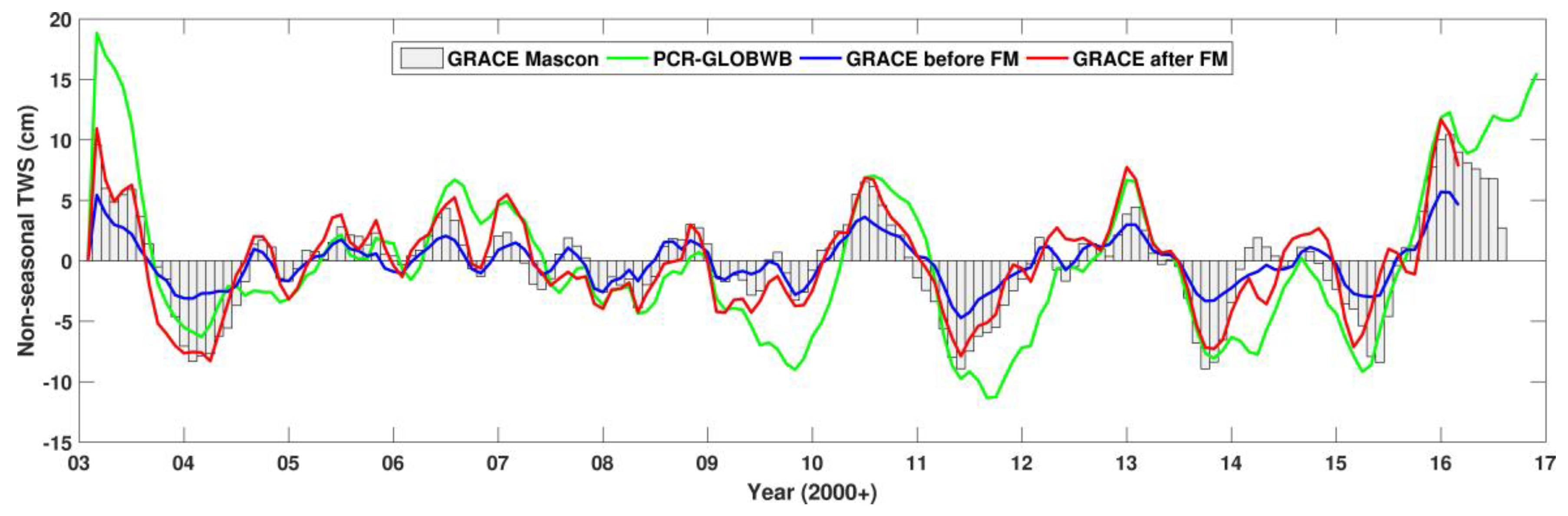
3.3. Comparison between Forward-Modeling, Mascon Grids, and Tellus Grids

The forward-modeling method is applied to estimate the GRACE TWS variations. For clarity, the GRACE TWS variations before and after applying forward-modeling are called GRACE before FM and GRACE after FM, respectively. In GRACE before FM, the time series of TWS presents a clear seasonal variation, ranging from approximately -5 cm to 5 cm (Figure 5). In GRACE after FM, the range of TWS variations extends to ± 15 cm, and the annual amplitude increases by a factor of 2.1 (see Table 2). For comparison, the TWS variations derived from CSR Release05 mascon products (“GRACE Mascon” in Figure 5) and GRACE Tellus grid products (“GRACE Tellus” in Figure 5) are also included in Figure 5. The “GRACE after FM” agrees well with the two independent products, particularly from January 2003 to March 2016 (see Figure 5). The correlation coefficient between “GRACE after FM” and “GRACE Mascon” reaches up to 0.93, and it is higher than that of “GRACE Tellus” (0.80). A better agreement of the former is likely due to that the forward-modeling method and mascon products are independent of external data. The PCR-GLOBWB model is also used to evaluate the GRACE result. The “GRACE after FM” and “GRACE Mascon” lie very close to PCR-GLOBWB. These consistent results somewhat infer the satisfactory performance of GRACE in revealing the synthetic gravity signals over the Poyang Lake basin.
Through the time series in Figure 5, the obvious overestimated TWSs are observed during the 2010 and 2016 flood period. To analyze the non-seasonal anomalous conditions of floods, the seasonal variations are removed from the original TWSs. The correlation coefficient between “GRACE Mascon” and “GRACE before FM” is 0.85. After forward-modeling is applied, the correlation coefficient increases to 0.93. It also demonstrates the good performance of the forward-modeling method. As shown in Figure 6, there are also long-term positive TWS anomalies during the rainy seasons in 2010 and 2016, consistent with the flood periods observed from Figure 5. As for the drought events, the long-term negative anomalies are seen during the dry season in 2011, reflecting the severe drought event over the Poyang Lake basin. However, no drought event is observed over the Poyang Lake basin in 2006, when the upper Yangtze River basin suffers a severe drought [2,46].

4. Flood Events Identification

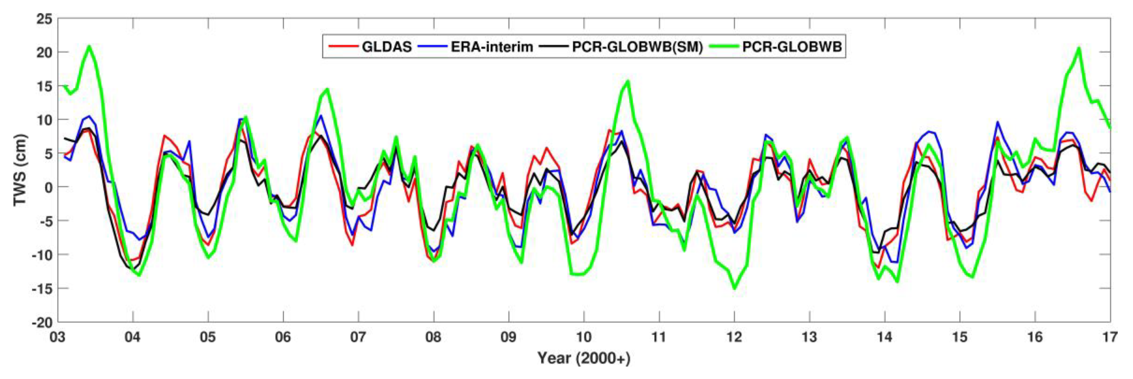
4.1. Hydrological Models

The TWS variations over the Poyang Lake basin are computed using three hydrological models (Figure 7). The soil moisture model of PCR-GLOBWB (i.e., PCR-GLOBWB (SM) in Figure 7) agrees well with GLDAS and ERA-interim models. The good agreement justifies the usage of the PCR-GLOBWB (SM) model to assess the soil moisture variations over the Poyang Lake basin. As the groundwater and surface component are also included, the greater amplitude of TWS variations (see Figure 7 and Table 2) is observed in PCR-GLOBWB. It demonstrates the extreme contribution of surface water and groundwater component to TWS over Poyang Lake basin [11]. Comparing the TWS variations derived from PCR-GLOBWB and PCR-GLOBWB(SM), the long-term positive TWS anomalies in Figure 6 are always corresponding to the big discrepancies between these two time series in Figure 7. The reason is that the SM storage is limited by a specific capacity with a certain condition value. During the flood period, the water is transferred from surface to groundwater. Note that there are always phase lags of approximately one month between PCR-GLOBWB and PCR-GLOBWB(SM). It infers that the surface water takes several weeks to infiltrate to lower layers. The same situation is also seen in 2003, when the high discrepancies are observed between PCR-GLOBWB and PCR-GLOBWB(SM). According to [47], the big discrepancies in 2003 are likely caused by the initial condition or the precipitation error, but not the flood event.
The different flood characteristics are observed in 2010 and 2016. In the dry season of 2009 (from September 2009 to February 2010), the continuous negative TWS anomalies (non-seasonal) derived from PCR-GLOBWB are seen Figure 6. It infers an extra capacity for the upcoming floods in 2010. By contrast, the continuous positive TWS anomalies are observed in the dry season of 2015 (from September 2015 to February 2016), indicating saturated water storages in all components. Similar signatures are also seen in the precipitation result (Section 4.3). This is likely the indication of the severest flood event in 2016.

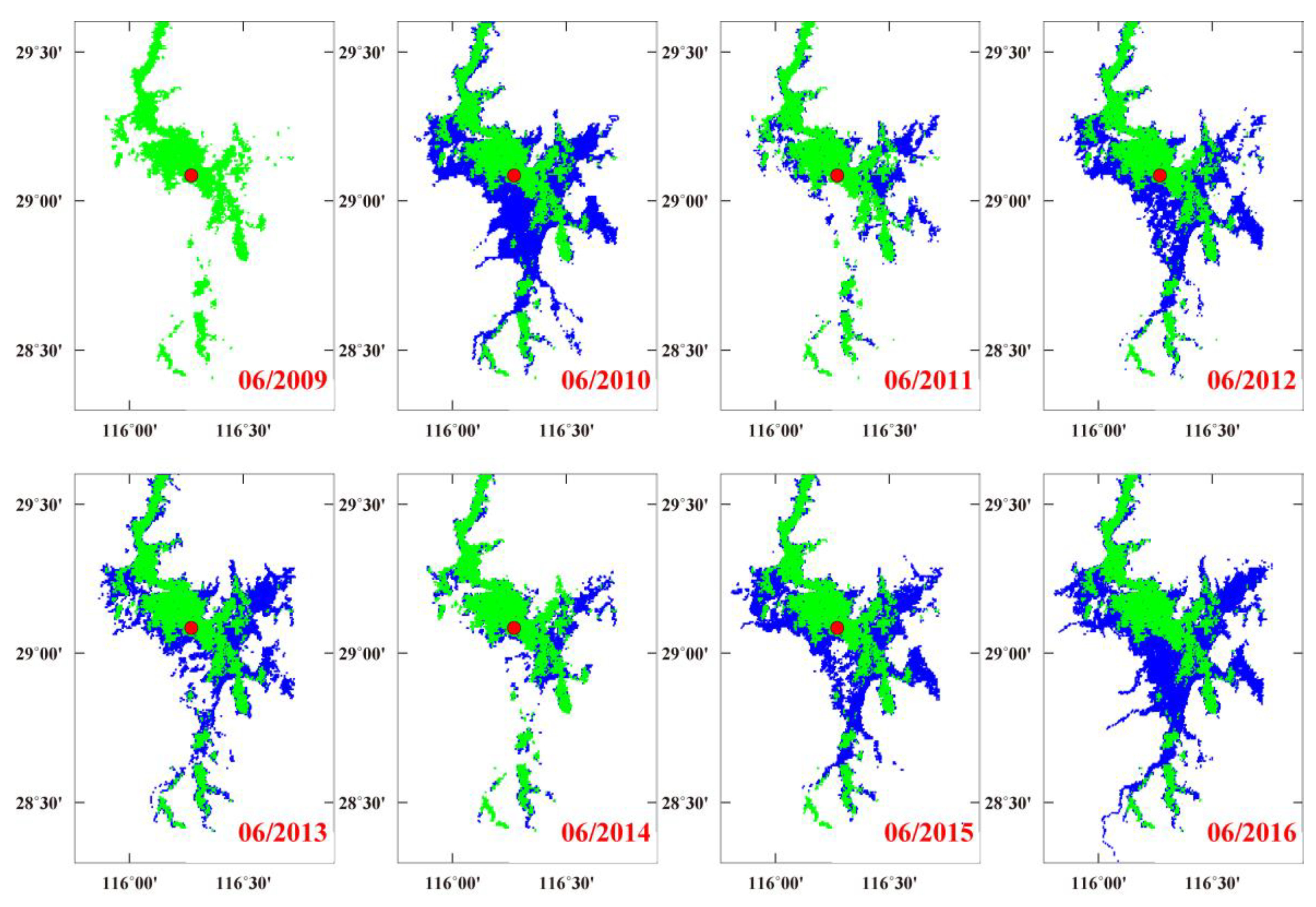
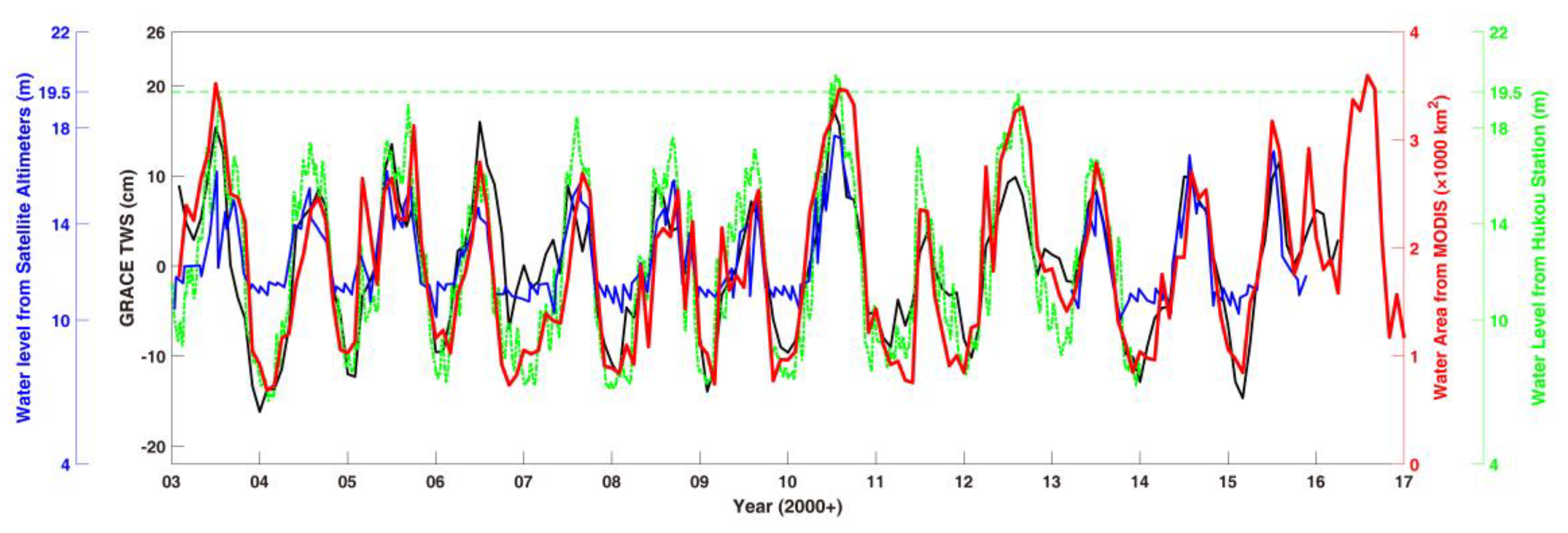
4.2. MODIS and Altimetry
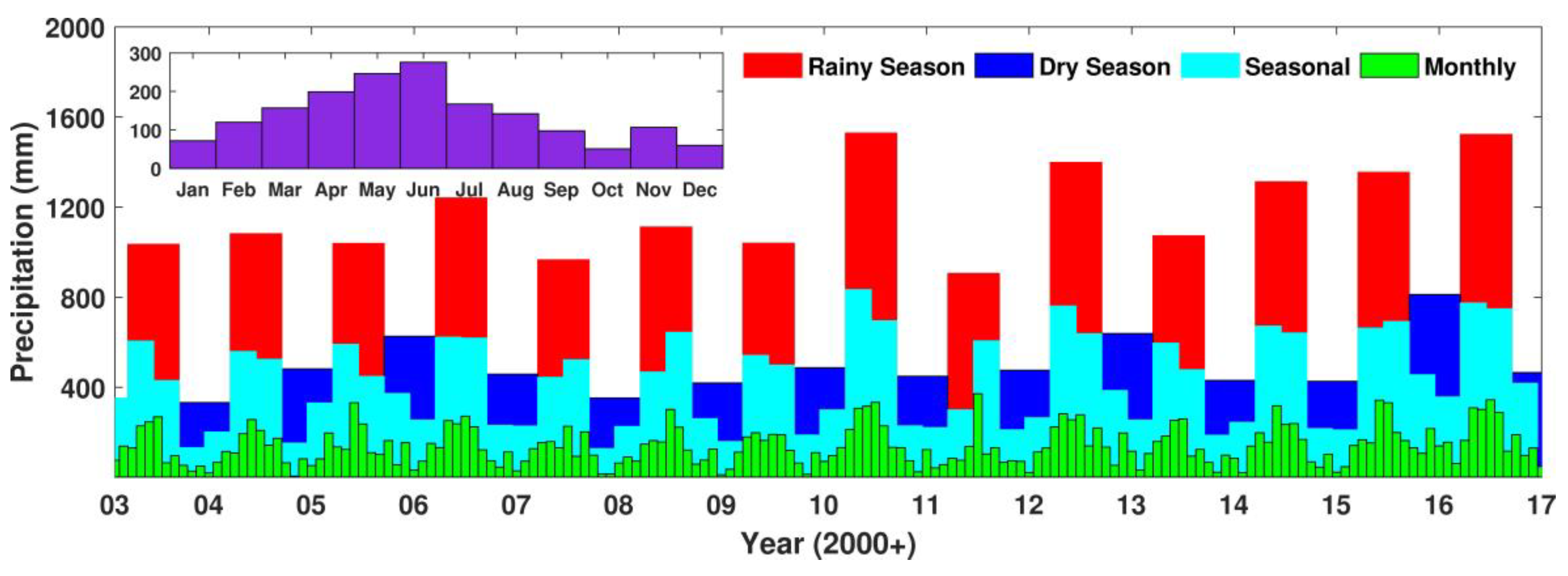
To analyze the inundated area variations of the Poyang Lake, the 8 day NDWI values are computed using the MODIS data, and the inundated areas are then computed via these NDWI values. As floods usually occur between June and August [3,5], the inundated areas in June between 2009 and 2016 are analyzed and presented in Figure 8. As seen in Figure 6, there is a significant negative TWS anomaly in June 2009. Therefore, the inundated area of June 2009 is used as a reference, quantified as only 1635.8 km2. In Figure 8, the largest inundated area is observed in June 2016. Comparing with the inundated area of 3270.8 km2 in June 2016, the second largest inundated area is 3185.8 km2 in June 2010, when the flood affects the regions along the Poyang Lake.
The monthly mean inundated area between January 2003 and December 2016 is used to analyze the intra-monthly and seasonal variability (Figure 9). The peak of the inundated areas is observed between June and August 2016, with a mean peak value of 3445.0 km2. The second largest long-term peak is detected between June and August 2010, with a mean peak value of 3370.3 km2. These peak values are 33% and 30% higher than the mean peak value between 2003 and 2016. These results are in good agreement with those derived from GRACE data and PCR-GLOBWB model: (1) the largest long-term positive peak of GRACE TWS variation (14.7 cm) is detected between June and August 2016, and the second positive peak (13.9 cm) is observed in 2010; (2) in terms of PCR-GLOBWB model derived TWS variations, the mean values in these two periods are 17.9 cm and 13.2 cm, respectively, also ranking the first and second during the whole study period.
In Figure 9, the GRACE TWS variations, the water levels derived from Altimetry satellites, and the water levels recorded at the Hukou hydrological station are compared. Besides the consistent peaks in 2010 and 2016, the temporal variations of GRACE and MODIS are also in a good agreement, with a correlation coefficient of 0.82. Note that MODIS data can only detect the inundated area variations over the Poyang Lake, while GRACE estimates the TWS variations over the whole basin. As shown in Figure 1, Poyang Lake receives water from five sub rivers in the lake basin, and these sub rivers almost flow through the whole Poyang Lake basin. Therefore, as implied by the strong correlation, the inundated areas of the Poyang Lake derived from MODIS can also partly reflect the TWS variations of the Poyang Lake basin.
In addition, the daily water levels observed by the Hukou station also show a good agreement with the MODIS-derived inundated areas, with a strong correlation (0.90). During the 2010 flood period, the water levels continuously exceed the warning level of 19.50 m (green dot horizontal line in Figure 9) for 25 days, with the highest level of 20.06 m on July 21, 2010. The highest water level (21.33 m) is observed on July 11, 2016, and the water levels continuously exceed the warning level for 28 days in this month. This can also support the MODIS-derived result, which presents the largest inundated area (3594.4 km2) in July 2016.
As seen in Figure 9, in the rainy season, the water levels derived from the altimetry satellites correspond well with those recorded by the hydrological station. The largest water level 17.68 m is also detected on July 11, 2016. However, in the dry seasons, the consistency of these two datasets is not as good as that in the rainy seasons. In the rainy seasons, the altimetry satellites records the water levels at the center of the Poyang Lake. By contrast, the altimetry data point exposes to the shore of the lake in the dry seasons, which can only reflect the height variations of lands instead of waters. This is likely the reason for the inconsistency between the altimetry-derived and hydrological observed water level.

4.3. TRMM

The precipitation over the Poyang Lake basin is analyzed using the TRMM 3B43 data. In Figure 10, the top three largest precipitations are observed in June of 2012, 2016, and 2010, with the monthly mean value of 372 mm, 344 mm, and 342 mm, respectively. As discussed earlier, the latter two periods are characterized as floods, based on the large inundated areas and high GRACE-derived TWS variations. The accumulations of precipitation in spring (March to May), summer (June to August), autumn (September to November), and winter (December to February) are also analyzed. The mean value of spring and summer is 602 mm and 584 mm, respectively, accounting for 35.6% and 34.6% of annual precipitation. The largest precipitation 833 mm (38.4% above mean value) is observed in spring 2010, which induces the 2010 flood.
The lowest precipitation in spring is observed in 2011 (299.2 mm), which causes a severe drought in this year. This can be supported by the long-term negative TWS anomalies in Figure 6. Therefore, although the heaviest storm hit Poyang Lake in June 2011, the inundated area of this month is only 2353.0 km2, ranking the sixth during 2009–2015 (Figure 8). In other words, with the largest precipitation, the flood in June 2011 is not as serious as those in 2010 and 2016 yet.
According to the mean precipitation of each month (inset figure in Figure 10), the meteorological year is divided into a rainy season (March to August) and a dry season (September to February). The rainy season accounts for 70.2% of the annual precipitation. To analyze the influence of the precipitation over the Poyang Lake, a comparison of the MODIS-derived inundated areas is made between the dry season and the rainy season (see Figure 11). In 2010 and 2012, the lake almost shrinks to a line in the dry season, while the central lake and the north outlet are connected in the rainy season. In Figure 10, the top three precipitations are observed in the rainy season of 2010, 2016, and 2012, with the accumulated value of 1528 mm, 1522 mm and 1398 mm, respectively. Although ranking the second in terms of precipitation in the rainy season, the inundated area is the largest in June 2016 (see Figure 11). This is likely due to the largest precipitation in the previous dry season (from August 2015 to February 2016). As seen in Figure 6, Figure 7, Figure 10 and Figure 11, the plenteous precipitation in the dry season of 2015 is also responsible for the positive GRACE TWS anomalies, the positive discrepancies between PCR-GLOBWB and other hydrological models, and the largest MODIS-derived inundated area in January 2016.

4.4. In Situ Data

The time series of temperature, precipitation, and evaporation observed by 24 meteorological stations are shown in Figure 12. The ground-based precipitations correspond well with those estimated by the TRMM data, with a correlation coefficient of 0.98. The difference between those two datasets may result from the different spatial resolution, which is 0.25 degrees for TRMM, but point-wise for the meteorological station. Therefore, the results (mainly in Section 4.3) derived from TRMM data are reliable over the Poyang Lake basin. Noted that there is no precipitation shortage in 2006, neither for TRMM data nor for meteorological station observations. It can be used to explain the absence of the drought event in this year over the Poyang Lake basin (see Figure 5 and Figure 6).
The evaporation is 219.6 mm in spring, only accounting for 21.4% of the annual amount. However, as discussed earlier, the precipitation accounts for 35.6% in spring. The heavy rainfall and weak evaporation facilitate the floods over the Poyang Lake basin in spring. It is also noteworthy that there is a marked drop of evaporation during 2014-2016 (Figure 12). For instance, the mean value in summer during this period is 307.7 mm, compared with 426.2 mm during 2003-2013. This can partly attribute to the lower temperature during 2014-2016, which decreases 1.3 °C and 0.8 °C in July and August compared to the mean value of 2003-2013. The decrease in temperature and evaporation in summer is likely the other reason for the most severe flood in 2016.
In terms of temperature in winter, the high (low) value seems to correspond to the upcoming flood (drought) event. For example, the lowest temperature is 2.4 °C in January 2011, which is significantly lower than the mean value (5.8 °C) of January during 2003-2016. This indicates a strong cool-dry current across the Poyang Lake basin, resulting in less precipitation and more severe drought. By contrast, the warm winter in 2010 (7.3 °C) and 2016 (6.6 °C) infers a strong warm-humid current across the Poyang Lake basin, leading to more precipitation and upcoming flood.

5. Discussion

In the GRACE data processing, the forward-modeling method is validated by the simulated GRACE onboard observations for the first time. In both spectral and spatial domains, the method has proven satisfactory performance in mitigating the leakage errors. After applying the forward-modeling method, the GRACE-derived TWS variations present more dramatic seasonal fluctuations. This enhances the ability of capturing the flood signals over the Poyang Lake basin. Actually, the global TWSs after forward-modeling also present very similar patterns with those of initial input temporal gravity model (not shown). However, the stopping criterion of the iteration is limited to the Poyang Lake basin, and the selection of filters’ parameters (e.g., Gaussian filter radius, de-correction filter parameters) may also affect the efficiency of this method. More studies about the performance of the forward-modeling method in the other regions, as well as the effect of different filters’ parameters are recommended in the future. In addition, many recent and ongoing studies have focused on the uncertainties of GRACE estimates [47,48,49,50,51]. The forward-modeling method has been used to quantify and understand the hydrologic processes in several specific regions [10,11,26,27,28,29]. Based on these previous works, the global analyses of the forward-modeling method approach are ongoing and will be discussed in the near future.
In the Poyang Lake basin, the GRACE estimates of TWS are also consistent with the estimates from alternative sources, such as the PCR-GLOBWB-derived TWS, MODIS-derived inundated area, and in situ water level. The comparisons show that the GRACE-derived TWSs perform well in flood detection over our study region. Note that, in this study, only the instantaneous analyses of the TWS estimates are used to identify the flood/drought events over the Poyang Lake basin. A number of recent studies have looked into the potential merit of long lead-time flood prediction [52,53]. These new techniques are also recommended to quantify and predict the flood events over the Poyang Lake basin.
The NDWI is used to delineate the inundated area, which is affected by the threshold used to separate the water from land pixels. To assess the accuracy of NDWI, as recommended by Feng et al. [5], a visual examination in the software ENVI is used to determine how the NDWI-based water/land interface contour fit the visually determined water and land objects in the RGB images. For most of the 478 cloud-free MODIS images, the NDWI performs well. In addition, as Feng et al. [5] have already estimated the inundated area variations between 2000 and 2010, we also compare our inundated area estimations with those listed in their work (Table 2 and Table 3 in Feng et al. [5]). An excellent agreement is found between these two results, with the coefficients (with 95% confidence bounds) of 0.98 and the R-square value of 0.94.
To assess the accuracy of MODIS-derived inundated area, the concurrent higher-resolution satellite imageries are always included for comparison [5,54]. In this study, the cloud-free Landsat-8 OLI (Operational Land Imager) image collected on 5 October 2013 is analyzed and compared with MODIS observations on 7 October 2013. The NDWI maps and their associated histograms are shown in Figure 13. The histograms show a similar bi-modal distribution for NDWI between MODIS and Landsat-8 images. The pixels with a NDWI value higher than 0 are clearly water. With the significantly higher resolution (30 m), the Landsat-8 image reveals more details and slight differences from the MODIS result for some lake segments, especially around the tributaries. However, the NDWI map from the two measurements presents a very similar pattern. As a result, the inundated areas from the two independent measurements are nearly equal, about 2121.2 km2 for MODIS and 2182.5 km2 for Landsat-8. In order to investigate the potential bias derived from different spatial resolutions, the Lansat-8 image is also resampled at 500 m of spatial resolution. As shown in Figure 13, the excellent agreement can also be found between three NDWI maps, as well as bi-modal histograms. Therefore, it appears to be reasonable that the medium-resolution (500 m) MODIS time-series data can provide valuable information to study short-term and long-term changes in the inundation characteristics of the Poyang Lake. However, in dry seasons (see Figure 11), some water bodies are disconnected in the MODIS result. It may limit the usage of the 500 m resolution MODIS data for studying the extreme narrow channel water variations. For our purpose, the estimation of the total inundation area, this potential artifact will not affect our results or interpretations.

6. Conclusions

In this study, multiple satellite remote sensing observations, hydrological models, and in situ data are used to characterize the flood events over the Poyang Lake basin between 2003 and 2016.
Among the satellite remote sensing observations, this study mainly focuses on GRACE, which observes the TWS variations directly. To mitigate the leakage error during the GRACE data processing, the forward-modeling method is applied. For the first time, the method is assessed using the contaminated noise onboard observations. In both spectral and spatial domains, the simulation results infer a good performance of this method on the suppression of high-frequency noise while reducing the signal loss. The forward-modeling method is then applied to the CSR Release05 monthly gravity data. The comparison results with the newly released CSR mascon grids infer the satisfactory performance of the forward-modeling method in reducing leakage errors. Comparing with other observations, the results show that GRACE data can be considered as an effective tool for monitoring a regional scale (1.622 × 10⁵ km2) hydrological basins. According to our validations and comparisons, the forward-modeling method improves the ability of GRACE-based estimates of capture the irregularly TWS signatures in the regional scale hydrological basins. In addition, as the forward-modeling method does not rely on external data, it is recommended to investigate the TWS variations in the regional scale hydrological basins.
The significant seasonal variations of the inundated area over the Poyang Lake are estimated with the MODIS surface reflectance data. The MODIS-derived inundated area presents a strong correlation with the in situ water level (0.90). The GRACE-derived TWS also agrees well with the MODIS-derived inundated area, with a correlation coefficient of 0.82. It demonstrates that surface reflectance data can also be used to estimate TWS at sub-monthly time scales. It also indicates the potential of the MODIS estimates to fill in the missing data between the termination of GRACE and the launch of the GRACE Follow-On mission [45]. Further studies about this issue are recommended after the launch of GRACE Follow-On in 2018.
The most severe flood can be identified in 2016 observed by multiple observations:
(1) TRMM observes the accumulated precipitation (1522 mm) in the rainy season of 2016;
(2) MODIS observes the largest inundated area (3594.4 km2) in July 2016;
(3) in situ data shows the longest warning-exceeded water levels (28 days) in July 2016;
(4) GRACE and PCR-GLOBWB detect the continuous positive TWS anomalies.
On the other hand, using multiple observations facilitates the interpretation of the flood event:
(1) there is an obvious positive temperature anomaly in the winter of 2016 (0.8 °C), inferring the strong warm-humid currents crossing the Poyang Lake basin;
(2) the MODIS-derived inundated area of January 2016 shows the maximum (1801.1 km2) among the Januaries between 2003 and 2016;
(3) influenced by plenteous precipitation events in the previous dry season, the continuous rain in spring and summer lead to the severest flood in 2016.
Given the continuous observations from various remote sensing missions and ground observation network, the method and analysis in this study may serve as a criterion to characterize the future flood events over the Poyang Lake basin. For the same reason, the multiple observations used here may be applied to other regions to study extreme hydrological activities.

Author Contributions

Hao Zhou, Zhicai Luo, and Zebing Zhou conceived and designed the research; Hao Zhou, Natthachet Tangdamrongsub, and Lijie He performed the experiments and analyzed the data; Hao Zhou and Lijie He wrote the paper; Chuang Xu, Qiong Li, and Yunlong Wu revised the paper.

Acknowledgments

GLDAS model can be obtained from https://mirador.gsfc.nasa.gov/. PCR-GLOBWB model can be obtained from https://github.com/UU-Hydro/PCR-GLOBWB_model. ERA-Interim model can be downloaded from https://www.ecmwf.int/. This work is financially supported by the National Natural Science Foundation of China (No. 41704012, 41474019, 41504014, 41504015, 41704011), the project funded by China Postdoctoral Science Foundation (Grant no. 2016M592337) and the Open Research Fund Program of the State Key Laboratory of Geodesy and Earth’s Dynamics (Grant no. SKLGED2017-1-2-E).

Conflicts of Interest

The authors declare no conflict of interest.

Appendix A

The dynamic approach was adopted during the forward-modeling method validation. This approach is formed on the basis of satellite motion equation. Using this equation, the integral orbits X ^ can be obtained through a numerical integrator, such as Runger-Kutta, Adams-Cowell and Gauss-Jackson integrator. During the orbit integration, the state vector of the first epoch is taken as the initial state vector X 0 , and the prior force models p (including static gravity field model, temporal gravity field model, tide model, non-tidal model, N-body perturbation, general relativistic effects, etc.) are exploited to estimate the conservative force at each epoch. Due to the uncertainties in initial state vector Δ X 0 and force models Δ p (mainly the earth’s gravity field model), there are inevitable differences Δ X between the integral orbits X ^ and those observed by GNSS receivers for real GRACE mission ( X ). Note that X represents simulated orbits in ‘Ture World’ in this study. Using the orbit differences, the observation equation of dynamic approach can be built as
Δ X = X X ^ = X X 0 Δ X 0 + X p Δ p
Similar to the orbit differences, the observation equation in terms of range rates ρ ˙ can be written as
Δ ρ ˙ = ρ ˙ ρ ˙ ^ = ρ ˙ X 0 A Δ X 0 A + ρ ˙ X 0 B Δ X 0 B + ρ ˙ p Δ p
where superscript A and B respectively represents GRACE A and GRACE B satellite, the partial derivatives X X 0 , X p , ρ ˙ X 0 A , ρ ˙ X 0 B and ρ ˙ p can also be estimated by numerical integrators. Combing Equations (A1) and (A2), the gravity field model can be updated by estimating Δ p with least square adjustment. Dividing the observations into monthly datasets, the monthly gravity field model, which reflects the mean mass transportations within one month, can be determined.
To quantify the efficiency of the forward-modeling method, we did a simulation study with our DynaSST software. This software has been successfully applied for the long-term static gravity field model HUST-Grace2016s estimation [38], the monthly gravity field model HUST-Grace2016 determination [11] and the future GRACE-type mission simulation [24]. The GRACE observations are simulated on the basis of real GRACE designed parameters, with an orbital height of 415.6 km, an initial inclination of 89.03 degrees and a mean inter-satellite range of 220 km. The corresponding orbit resonance of 463/30 can guarantee the dense distribution of observations. During the simulation, the ‘real observations’ ( X in Equation (A1) and ρ ˙ in Equation (A2)) are integrated with the simulation force models in ‘True World’ (see Table 1), while the ‘reference observations’ ( X ^ in Equation (A1) and ρ ˙ ^ in Equation (A2)) are integrated with the simulation force models in ‘Reference World’ (see Table 1). In addition, the measurement errors (including orbit errors and range rate errors) are also taken into consideration (see Table 1).
After estimating the monthly temporal gravity field models, the degree variances of geoid heights σ l (see Figure 3) are introduced to assess the power of signals and errors in the spectral domain,
σ l = R E m = 0 l ( Δ C l m 2 + Δ S l m 2 )
where Δ C l m and Δ S l m are the coefficient differences between the estimated model and the static gravity field model in ‘True World’, l and m is respectively the degree and order of SHCs.

References

  1. Zhang, Q.; Sun, P.; Chen, X.; Jiang, T. Hydrological extremes in the Poyang Lake basin, China: Changing properties, causes and impacts. Hydrol. Process. 2011, 25, 3121–3130. [Google Scholar] [CrossRef]
  2. Zhang, Z.; Chao, B.; Chen, J.; Wilson, C.R. Terrestrial water storage anomalies of Yangtze River Basin droughts observed by GRACE and connections with ENSO. Glob. Planet. Chang. 2015, 126, 35–45. [Google Scholar]
  3. Guo, H.; Hu, Q.; Jiang, T. Annual and seasonal streamflow responses to climate and land-cover changes in the Poyang Lake basin. China. J. Hydrol. 2008, 355, 106–122. [Google Scholar] [CrossRef]
  4. Li, X.; Ye, X. Spatiotemporal Characteristics of Dry-Wet Abrupt Transition Based on Precipitation in Poyang Lake Basin, China. Water 2015, 7, 1943–1958. [Google Scholar] [CrossRef]
  5. Feng, L.; Hu, C.; Chen, X.; Cai, X.; Tian, L.; Gan, W. Assessment of inundation changes of Poyang Lake using MODIS observations between 2000 and 2010. Remote Sens. Environ. 2012, 121, 80–92. [Google Scholar] [CrossRef]
  6. Feng, L.; Hu, C.; Chen, X.; Li, R.; Tian, L.; Murch, B. MODIS observations of the bottom topography and its inter-annual variability of Poyang Lake. Remote Sens. Environ. 2011, 115, 2729–2741. [Google Scholar] [CrossRef]
  7. Shang, H.; Jia, L.; Menenti, M. Analyzing the inundation pattern of the Poyang Lake floodplain by passive microwave data. J. Hydrometeorol. 2015, 16, 652–667. [Google Scholar] [CrossRef]
  8. Cai, X.; Feng, L.; Wang, Y.; Chen, X. Influence of the Three Gorges Project on the water resource components of Poyang Lake watershed: observations from TRMM and GRACE. Adv. Meteorol. 2015, 3, 1–7. [Google Scholar] [CrossRef]
  9. Vermote, E.F.; Kotchenova, S.Y.; Ray, J.P. MODIS Surface Reflectance User’s Guide Version 1.3. 2011. Available online: http://modis-sr.ltdri.org/guide/MOD09_UserGuide_v1_3.pdf (accessed on 5 February 2018).
  10. Tangdamrongsub, N.; Ditmar, P.G.; Steele-Dunne, S.C.; Gunter, B.C.; Sutanudjaja, E.H. Assessing total water storage and identifying flood events over Tonlé Sap basin in Cambodia using GRACE and MODIS satellite observations combined with hydrological models. Remote Sens. Environ. 2016, 181, 162–173. [Google Scholar] [CrossRef]
  11. Zhou, H.; Luo, Z.; Tangdamrongsub, N.; Wang, L.; He, L.; Xu, C.; Li, Q. Characterizing drought and flood events over the Yangtze River Basin using the HUST-Grace2016 solution and ancillary data. Remote Sens. 2017, 9, 1100. [Google Scholar] [CrossRef]
  12. Schwatke, C.; Dettmering, D.; Bosch, W.; Seitz, F. DAHITI—An innovative approach for estimating water level time series over inland waters using multi-mission satellite altimetry. Hydrol. Earth Syst. Sci. 2015, 19, 4345–4364. [Google Scholar] [CrossRef]
  13. Kummerow, C.; Barnes, W.; Kozu, T.; Shiue, J.; Simpson, J. The tropical rainfall measuring mission (TRMM) sensor package. J. Atmos. Ocean. Tech. 1998, 15, 809–817. [Google Scholar] [CrossRef]
  14. Longuevergne, L.; Wilson, C.R.; Scanlon, B.R.; Crétaux, J.F. GRACE water storage estimates for the Middle East and other regions with significant reservoir and lake storage. Hydrol. Earth Syst. Sci. 2013, 17, 4817–4830. [Google Scholar] [CrossRef] [Green Version]
  15. Eicker, A.; Forootan, E.; Springer, A.; Longuevergne, L.; Kusche, J. Does grace see the terrestrial water cycle “intensifying”? J. Geophys. Res. 2016, 121, 733–745. [Google Scholar] [CrossRef]
  16. Feng, W.; Zhong, M.; Lemoine, J.M.; Biancale, R.; Hsu, H.; Xia, J. Evaluation of groundwater depletion in north china using the gravity recovery and climate experiment (GRACE) data and ground-based measurements. Water Resour. Res. 2013, 49, 2110–2118. [Google Scholar] [CrossRef]
  17. Long, D.; Shen, Y.; Sun, A.; Hong, Y.; Longuevergne, L.; Yang, Y. Drought and flood monitoring for a large karst plateau in Southwest China using extended GRACE data. Remote Sens. Environ. 2014, 155, 145–160. [Google Scholar] [CrossRef]
  18. Pan, Y.; Zhang, C.; Gong, H.; Yeh, P.J.; Shen, Y.; Guo, Y.; Huang, Z.; Li, X. Detection of human-induced evapotranspiration using GRACE satellite observations in the Haihe River basin of China. Geophys. Res. Lett. 2016, 44, 190–199. [Google Scholar] [CrossRef]
  19. Tapley, B.D.; Bettadpur, S.; Ries, J.C.; Thompson, P.F.; Watkins, M.M. GRACE measurements of mass variability in the earth system. Science 2004, 305, 503–505. [Google Scholar] [CrossRef] [PubMed]
  20. Jekeli, C. Alternative Methods to Smooth the Earth’s Gravity Field; Scientific report, 327; School of Earth Science, The Ohio State University: Columbus, OH, USA, 1981. [Google Scholar]
  21. Swenson, S.C.; Wahr, J. Post-processing removal of correlated errors in GRACE data. Geophys. Res. Lett. 2006, 33, L08402. [Google Scholar] [CrossRef]
  22. Guo, J.Y.; Duan, X.J.; Shum, C.K. Non-isotropic Gaussian smoothing and leakage reduction for determining mass changes over land and ocean using GRACE data. Geophys. J. Int. 2010, 181, 290–302. [Google Scholar] [CrossRef]
  23. Long, D.; Yang, Y.; Wada, Y.; Hong, Y.; Liang, W.; Chen, Y. Deriving scaling factors using a global hydrological model to restore GRACE total water storage changes for China’s Yangtze River Basin. Remote Sens. Environ. 2015, 168, 177–193. [Google Scholar] [CrossRef]
  24. Zhou, H.; Luo, Z.; Wu, Y.; Li, Q.; Xu, C. Impact of geophysical model error for recovering temporal gravity field model. J. Appl. Geophys. 2016, 130, 177–185. [Google Scholar] [CrossRef]
  25. Chen, J.L.; Famiglietti, J.S.; Scanlon, B.; Rodell, M. Groundwater storage changes: present status from GRACE observations. Surv. Geophys. 2016, 37, 397–417. [Google Scholar] [CrossRef]
  26. Chen, J.L.; Li, J.; Zhang, Z.; Ni, S. Long-term groundwater variations in Northwest India from satellite gravity measurements. Global Planet. Chang. 2014, 116, 130–138. [Google Scholar] [CrossRef]
  27. Chen, J.L.; Wilson, C.R.; Tapley, B.D. Contribution of ice sheet and mountain glacier melt to recent sea level rise. Nat. Geosci. 2013, 6, 549–552. [Google Scholar] [CrossRef]
  28. Jin, S.; Zou, F. Re-estimation of glacier mass loss in Greenland from GRACE with correction of land-ocean leakage effects. Global Planet. Chang. 2015, 135, 170–178. [Google Scholar] [CrossRef]
  29. Wu, Y.; Li, H.; Zou, Z.B. Investigation of water storage variation in the Heihe River using the Forward-Modeling method. Chin. J. Geophys. 2015, 58, 3507–3516. [Google Scholar]
  30. Chen, J.L.; Wilson, C.R.; Li, J.; Zhang, Z. Reducing leakage error in grace-observed long-term ice mass change: A case study in west Antarctica. J. Geod. 2015, 89, 925–940. [Google Scholar] [CrossRef]
  31. Landerer, F.W.; Swenson, S.C. Accuracy of scaled GRACE terrestrial water storage estimates. Water Resour. Res. 2012, 48, W04531. [Google Scholar] [CrossRef]
  32. Save, H.; Bettadpur, S.; Tapley, B.D. High-resolution CSR GRACE RL05 mascons. J. Geophys. Res. 2016, 121, 7547–7569. [Google Scholar] [CrossRef]
  33. Rodell, M.; Houser, P.; Jambor, U.E.A.; Gottschalck, J.; Mitchell, K.; Meng, C. The global land data assimilation system. Bull. Am. Meteorol. Soc. 2004, 85, 381–394. [Google Scholar] [CrossRef]
  34. Dee, D.P.; Uppala, S.M.; Simmons, A.J.; Berrisford, P.; Poli, P.; Kobayashi, S. The ERA-interim reanalysis: Configuration and performance of the data assimilation system. Q. J. Roy. Mmteor. Soc. 2011, 137, 553–597. [Google Scholar] [CrossRef]
  35. Wada, Y.; Wisser, D.; Bierkens, M.F.P. Global modeling of withdrawal, allocation and consumptive use of surface water and groundwater resources. Earth Syst. Dynam. 2014, 5, 15–40. [Google Scholar] [CrossRef]
  36. Tangdamrongsub, N.; Steele-Dunne, S.C.; Gunter, B.C.; Ditmar, P.G.; Sutanudjaja, E.H.; Sun, Y. Improving estimates of water resources in a semi-arid region by assimilating GRACE data into the PCR-GLOBWB hydrological model. Hydrol. Earth Syst. Sci. 2017, 21, 2053–2074. [Google Scholar] [CrossRef]
  37. Bettadpur, S. Gravity Recovery and Climate Experiment UTCSR Level-2 Processing Standards Document for Level-2 Product Release 0005; Center for Space Research, University of Texas: Austin, TX, USA, 2012. [Google Scholar]
  38. Zhou, H.; Luo, Z.; Zhou, Z.; Zhong, B.; Hsu, H. HUST-Grace2016s: A new GRACE static gravity field model derived from a modified dynamic approach over a 13-year observation period. Adv. Space Res. 2017, 60, 597–611. [Google Scholar] [CrossRef]
  39. Swenson, S.C.; Chambers, D.; Wahr, J. Estimating geocenter variations from a combination of GRACE and ocean model output. J. Geophys. Res. 2008, 113, B08410. [Google Scholar] [CrossRef]
  40. Cheng, M.; Tapley, B. Variations in the Earth’s oblateness during the past 28 years. J. Geophys. Res. 2004, 109, B09402. [Google Scholar] [CrossRef]
  41. Wahr, J.; Molenaar, M.; Bryan, F. Time variability of the Earth’s gravity field: Hydrological and oceanic effects and their possible detection using GRACE. J. Geophys. Res. 1998, 103, 30205–30229. [Google Scholar] [CrossRef]
  42. McFeeters, S.K. The use of the normalized difference water index (NDWI) in the delineation of open water features. Int. J. Remote Sens. 1996, 17, 1425–1432. [Google Scholar] [CrossRef]
  43. Huffman, G.J.; Bolvin, D.T. TRMM and Other Data Precipitation Data Set Documentation. Technical report; 2017. Available online: https://pmm.nasa.gov/sites/default/files/document_files/3B42_3B43_doc_V7_4_19_17.pdf (accessed on 5 February 2018).
  44. Tapley, B.D.; Bettadpur, S.; Watkins, M.; Riegber, C. The gravity recovery and climate experiment: Mission overview and early results. Geophys. Res. Lett. 2004, 31, L06619. [Google Scholar] [CrossRef]
  45. Flechtner, F.; Morton, P.; Watkins, M.; Webb, F. Status of the GRACE Follow-on Mission. IAG Symposium Gravity, Geoid, and Height Systems; Springer: Venice, Italy, 2014. [Google Scholar]
  46. Yao, C.; Luo, Z.; Wang, H.; Li, Q.; Zhou, H. GRACE-derived terrestrial water storage changes in the inter-basin region and its possible influencing factors: A case study of the Sichuan Basin, China. Remote Sens. 2016, 8, 444. [Google Scholar] [CrossRef]
  47. Scanlon, B.R.; Zhang, Z.; Save, H.; Sun, A.Y.; Schmied, H.M.; Beek, L.P.H.V.; Wiese, D.N.; Wada, Y.; Long, D.; Reedy, R.C.; et al. Global models underestimate large decadal declining and rising water storage trends relative to grace satellite data. Proc. Natl. Acad. Sci. USA 2018, 115, E1080–E1089. [Google Scholar] [CrossRef] [PubMed]
  48. Scanlon, B.R.; Zhang, Z.; Save, H.; Wiese, D.N.; Landerer, F.W.; Long, D.; Chen, J.; Longuevergne, L. Global evaluation of new GRACE mascon products for hydrologic applications. Water Resour. Res. 2016, 52, 9412–9429. [Google Scholar] [CrossRef]
  49. Wiese, D.N.; Landerer, F.W.; Watkins, M.M. Quantifying and reducing leakage errors in the JPL RL05M GRACE mascon solution. Water Resour. Res. 2016, 52, 7490–7502. [Google Scholar] [CrossRef]
  50. Long, D.; Longuevergne, L.; Scanlon, B.R. Global analysis of approaches for deriving total water storage changes from GRACE satellites. Water Resour. Res. 2015, 51, 2574–2594. [Google Scholar] [CrossRef] [Green Version]
  51. Long, D.; Pan, Y.; Zhou, J.; Chen, Y.; Hou, X.; Hong, Y.; Scanlon, B.R.; Longuevergne, L. Global analysis of spatiotemporal variability in merged total water storage changes using multiple GRACE products and global hydrological models. Remote Sens. Environ. 2017, 192, 198–216. [Google Scholar] [CrossRef]
  52. Reager, J.; Thomas, B.; Famiglietti, J. River basin flood potential inferred using GRACE gravity observations at several months lead time. Nat. Geosci. 2014, 7, 588–592. [Google Scholar] [CrossRef]
  53. Sun, A.Y.; Scanlon, B.R.; AghaKouchak, A.; Zhang, Z. Using GRACE Satellite gravimetry for assessing large-scale hydrologic extremes. Remote Sens. 2017, 9, 1287. [Google Scholar] [CrossRef]
  54. Normandin, C.; Frappart, F.; Lubac, B.; Bélanger, S.; Marieu, V.; Blarel, F.; Guiastrennec-Faugas, L. Quantification of surface water volume changes in the Mackenzie Delta using satellite multi-mission data. Hydrol. Earth Syst. Sci. 2018, 22, 1543. [Google Scholar] [CrossRef]
Figure 1. The study region of the Poyang Lake basin. The shape file of Poyang Lake, rivers and basin are obtained from the website of National Earth System Science Data Sharing Infrastructure (http://www.geodata.cn/). Hukou hydrological station and 24 meteorological stations are also shown. The red point over Poyang Lake represents the location of Altimetry data point. The inset map shows the location of the Poyang Lake basin in the Yangtze River basin.
Remotesensing 10 00713 g001
Figure 2. Flowchart of forward-modeling method.
Remotesensing 10 00713 g002
Figure 3. Monthly gravity field models in terms of degree variances of geoid heights derived from Strategy 1 (black) and Strategy 2 (red), respectively. The original GLDAS (blue) and the “original models” determined by different strategies are shown in solid lines. The models processed by the combined filter are shown in dashed lines, while those processed by the forward-modeling method are in dotted lines.
Remotesensing 10 00713 g003
Figure 4. TWS variations over Poyang Lake basin (black boundary) derived from different monthly gravity field models. (a) GLDAS model; (b) “original models”; (c) models after combined filtering; and (d) models after forward-modeling. The results in the first row (b1,c1,d1) are derived from models related to Strategy 1, and those in the second row (b2,c2,d2) are derived from models related to Strategy 2.
Remotesensing 10 00713 g004
Figure 5. TWS variations over the Poyang Lake basin derived from different GRACE solutions and PCR-GLOBWB model.
Remotesensing 10 00713 g005
Figure 6. Non-seasonal TWS variations over the Poyang Lake basin derived from GRACE solutions and PCR-GLOBWB.
Remotesensing 10 00713 g006
Figure 7. TWS variations derived from hydrological models.
Remotesensing 10 00713 g007
Figure 8. Inundated areas derived from MYD09A1 over Poyang Lake in June between 2008 and 2016 (blue). The green pixels represent the inundated regions in June 2009 used for comparison. The red point represents the location of the Altimetry data point.
Remotesensing 10 00713 g008
Figure 9. Water inundated area (derived from MODIS), water level (derived from satellite altimeters and Hukou station) and GRACE TWS variations (after forward-modeling) during 2003–2017. Each time series corresponds to the axes with the same color. The green dashed horizontal line represents the warning water level 19.50 m at the Hukou station.
Remotesensing 10 00713 g009
Figure 10. Monthly and seasonal precipitation over the Poyang Lake basin observed by TRMM 3B43. The meteorological season precipitation (“Seasonal” shown as cyan columns) was the summation of monthly data during March– May, June–August, September–November, and December–February.
Remotesensing 10 00713 g010
Figure 11. Inundated areas derived from MYD09A1 over Poyang Lake in January (green) and June (blue) of 2010, 2012, and 2016. The red point represents the location of Altimetry data point.
Remotesensing 10 00713 g011
Figure 12. Monthly mean temperature (cyan line), evaporation (black line) and precipitation (red column) observed by meteorological stations over the Poyang Lake basin during 2003–2016, compared with GRACE-derived TWS (red line), TRMM-derived precipitation (blue column), and water level observed at Hukou station (green dot line). The gray shades represent the flood periods.
Remotesensing 10 00713 g012
Figure 13. NDWI map and associated histogram for (a) MODIS image at 500 m of spatial resolution, (b) Landsat-8 image resampled at 500 m of spatial resolution and (c) Lansat-8 image at 30 m of spatial resolution.
Remotesensing 10 00713 g013
Table 1. Simulation force models and simulation strategies for the validation of the forward-modeling method. The simulation force models are all truncated to degree and order 60.
Simulation force modelsTrue WorldReference World
Static gravity field modelEIGEN-6C4GO_CON_GCF_2_DIR_R5
Temporal gravity field modelGLDASNone
Ocean tide modelEOT11aEOT08a
Non-tidal modelAOD1B RL05AOD1B RL04
Simulation Strategies~Strategy 1 (Current GRACE-type Mission)
Orbit noise2 cmNone
Range rate noise2.5 × 10−7 m/sNone
Simulation Strategies~Strategy 2 (Future GRACE-type Mission)
Orbit noise2 cmNone
Range rate noise5.0 × 10−8 m/sNone
Table 2. Annual amplitude (cm) and annual phase (month) of GRACE solutions and hydrological models. Correlation coefficients between GRACE TWS and TWS derived from PCR-GLOBWB and from “GRACE after FM” are also provided.
Annual AmplitudeAnnual
Phase
Correlation Coefficients w.r.t. PCR-GLOBWBCorrelation Coefficients w.r.t. GRACE after FM
GRACE before FM3.34 ± 0.380.91 ± 0.130.730.91
GRACE after FM7.05 ± 0.790.80 ± 0.060.78-
GRACE Tellus6.51 ± 0.720.72 ± 0.070.680.80
GRACE Mascon9.20 ± 1.020.79 ± 0.050.720.93
GLDAS-Noah5.58 ± 0.610.62 ± 0.070.700.79
ERA-Interim5.69 ± 0.620.59 ± 0.070.680.88
PCR-GLOBWB(SM)3.97 ± 0.430.76 ± 0.050.750.70
PCR-GLOBWB7.14 ± 0.780.82 ± 0.06-0.78

