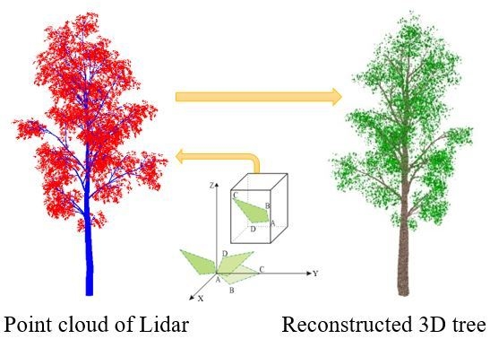
Reconstruction of Single Tree with Leaves Based on Terrestrial LiDAR Point Cloud Data


State Key Laboratory of Remote Sensing Science, Jointly Sponsored by Beijing Normal University and Institute of Remote Sensing and Digital Earth of Chinese Academy of Sciences, Beijing Engineering Research Center for Global Land Remote Sensing Products, Faculty of Geographical Science, Beijing Normal University, Beijing 100875, China
*
Author to whom correspondence should be addressed.
Remote Sens. 2018, 10(5), 686; https://doi.org/10.3390/rs10050686
Submission received: 12 December 2017
/
Revised: 7 March 2018
/
Accepted: 25 April 2018
/
Published: 28 April 2018
(This article belongs to the Special Issue Advances in Quantitative Remote Sensing in China – In Memory of Prof. Xiaowen Li)
Abstract
:Many studies have been focusing on reconstructing the branch skeleton of a three-dimensional (3D) tree structure that is based on photos or point clouds scanned by a terrestrial laser scanner (TLS), but leaves, as the important component of a tree, are often ignored or simplified because of their complexity. Therefore, we develop a voxel-based method to add leaves to a reconstructed 3D branches structure based on TLS point clouds. The location and size of each leaf depend on the spatial distribution and density of leaves points in the voxel. We reconstruct a small 3D scene with four realistic 3D trees and a virtual tree (including trunk, branches, and leaves), and validate the structure of each tree through the directional gap fractions calculated based on simulated point clouds of this reconstructed scene by the ray-tracing algorithm. The results show good coherence with those from measured point clouds data. The relative errors of the directional gap fractions are no more than 4.1%, though the method is limited by the effects of point occlusion. Therefore, this method is shown to give satisfactory consistency both visually and in the quantitative evaluation of the 3D structure.
1. Introduction
The three-dimensional (3D) structure of trees, including trunk, branch, and foliage elements, is important and fundamental data for the study of forest management [1], forest ecosystems [2], and vegetation radiative transfer models [3,4].
The development of quantitative remote sensing has led to a greater focus on the real structure of ground objects, especially the vegetation structures in various radiative transfer models. Early one-dimensional (1D) radiative transfer (RT) models, such as SAIL [5] and Suits [6], were developed based on K-M theory [7], and assumed horizontally homogeneous canopies, an approach that ignored the 3D structural characteristics of the canopies. Later, Li et al. [8,9] developed geometric-optical (GO) models that simplified the crown structures to a spheroid for a broadleaf tree or a cone for a coniferous tree to capture the 3D characteristics of forests on a coarse scale. Thereafter, a four-scale bidirectional reflectance model took into account the influence of non-uniform distributions (such as clumping effect) of branches and shoots in a conifer forest, or the “leaves” in the crowns of a broadleaf forest on the bidirectional reflectance distribution function (BRDF) [10]. Meanwhile computer simulation models were developed based on explicit 3D virtual canopy scenes to simulate the canopy reflectance by using ray-tracing or radiosity theory [11,12,13,14,15].
Compared to the RT and GO models, computer simulation models take advantage of computer graphics algorithms to eliminate many hypotheses and statistical rules of canopy structure and, as a result, improve the simulation accuracy greatly. However, explicit 3D structural canopy scenes are often required as fundamental input parameters and are complex and difficult to be constructed. Therefore, some computer simulation models use simplified 3D canopy structures. For example, the scenes that are used in the DART model [16] comprise many small voxels with statistical foliage properties rather than a detailed leaf and branch structure. Huang et al. [17] simplified the detail structures of individual tree crowns to some porous thin objects in the RAPID model, which can simplify the representation of canopy structures and decrease the computing time. All of these simplifications assumed that the statistical canopy structure would provide the same scattering behavior as the explicit 3D situation. However, Disney et al. [18] had point out that simplified canopy scenes may cause an inherent loss of information. Widlowski et al. [19] found that architectural simplifications may have an impact on the fidelity of simulated satellite observations at the bottom of the atmosphere for a variety of spatial resolutions, spectral bands, and viewing and illumination geometries.
For these reasons, the simple statistical parameters for crown structure (such as LAI-leaf area index, LAD-leaf angle distribution) have been unable to satisfy the requirements of quantitative remote sensing research. The latest simulation from the Radiative Transfer Model Intercomparision Initiative (RAMI-http://rami-benchmark.jrc.ec.europa.eu/HTML/) increased the number of actual structural canopy scenes. This reflects the trend toward the development of remote sensing for vegetation. However, it is still difficult to acquire accurate 3D geometry and topology information for a real tree due to the complexity of the tree structure.
The development of terrestrial laser scanner (TLS) technology enables the use of point clouds that were scanned from trees to estimate the structural parameters for single trees or forests, including LAI, LAD [20], and leaf area density [21]. Additionally, point clouds are also used to reconstruct 3D trees. Most studies pay more attention to the reconstruction of branch skeletons [22,23,24]. An overview of this area can be found in a review from Huang et al. [25].
Only a few methods reconstructed a whole tree by adding leaves or needles to the reconstructed branches. For example, Xu et al. [26] assumed that the leaf density in a real tree was uniform and determined leaf locations using the number of feasible skeleton nodes that existed within a certain distance. This method requires that even small branches be reconstructed with high accuracy. Livny et al. [23] created leaves next to each leaf node in the branch-structure graph (BSG) and generated a random number between 20 and 50 leaves that were randomly placed within a sphere that was centered on the leaf node. They then added textures to the reconstructed geometry to enhance visual appeal. Côté et al. [27] added foliage to reconstruct conifer trees by repeatedly testing the radiation, reflectance characteristics, and gap fraction of canopy. Their method can reconstruct 3D trees with structural and radiative consistency.
These methods of adding leaves have not made full use of the spatial information obtained from foliage point cloud distributions. In this study, an easy method for reconstructing realistic 3D trees (including trunk, branches, and leaves) is developed. This method is based on aligned point clouds that were scanned from multiple sites and combined information regarding the spatial distribution of points with retrieved structural parameters. The reconstructed trees can meet the basic demands of computer simulation models and maintain a directional gap fraction that is consistent with that of the real ones.
2. Experiment and Datasets
2.1. Study Area
The experimental field located in an open and flat prairie in Chengde city, Hebei Province, China (42°14’28.7”N, 117°04’57.29”E) is covered by the dominant grassland and scattered bushes and trees under the typical continental monsoon climate with an average annual temperature of −1.4 °C.
Four broadleaf, deciduous elm trees (Ulmaceae) with 6.0–7.5 m height and 15–25 cm diameters at breast (DBH) showed in the field center that was accompanied by approximately 3 cm understory sparse grasses. They had green leaves and a rough, dark, greyish-brown bark in summer. Some leaves were harvested and scanned with a laser scanner, and the average and maximum single-leaf areas were approximately 12 cm2 and 20 cm2, respectively.
2.2. Data Acquisition
2.2.1. Point Clouds of TLS
The experimental field was scanned by a TLS system, which included a laser scanner (Riegl VZ-1000 http://www.riegl.com) and a high-quality digital camera (Nikon D300s, Nikon Inc., Tokyo, Japan), on the 25 July 2014. The digital camera and the laser scanner were mounted together on one tripod with a pan-and-tilt platform, and a series of high-resolution color digital photographs and their accompanying point clouds were collected synchronously.
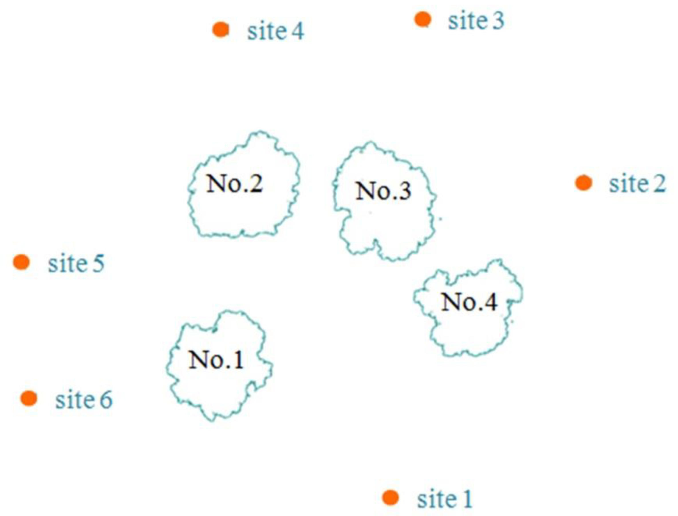
The scanning angular step was set to 0.03° and the laser scanner height was about 1 m above the ground. Six groups of point clouds were scanned from six sites around the field (Figure 1). All of the point cloud data were exported as ASCII files using the RiSCAN PRO software (http://www.riegl.com), a companion software package for the RIEGL Terrestrial 3D Laser Scanner Systems. The items in the file recorded each returned point’s location (XYZ coordination), distance (range [m]), beam direction (zenith and azimuth angle), reflectance (intensity), etc.
2.2.2. UAV Photographs
A six-rotor unmanned aerial vehicle (UAV) carried on a small, color digital camera was used to take RGB photographs (1024 pixel * 1024 pixel) of the experimental field from multiple view directions. The flight height of the UAV was approximately 50 m. One clear photograph taken in nadir was used in this study.
2.3. Point Cloud Data Processing
2.3.1. Elimination of Noisy Points.
Generally, there are noise points in the point cloud data due to the environment and the scanner itself, which can affect the accuracy of the retrieved canopy structural parameters and the 3D tree reconstruction. For example, ghost points occur when the laser beam hits the edge of an object. Two or more returned points will be recorded by the scanner, but with the wrong distance or intensity information. Therefore, a pre-processing step was included to eliminate ghost points.
We assume that each laser pulse will be reflected once it hits an object. Later returned signals with the same or similar beam directions are taken as ghost points, and should be deleted. First, all points are grouped into many small rectangular pyramids based on the range of zenith and azimuth angles within the width of a scanning angular step (δ). For example, the ith rectangular pyramid has the zenith range [θi − δ/2, θi + δ/2) and azimuth range [φi − δ/2, φi + δ/2). Where θi and φi are the zenith and azimuth of the ith scanning beam. The first data point in the pyramid is kept, but the others are deleted.
2.3.2. Classification
Point clouds can be classified using geometric information [28] or intensities [29]. In this study, all the point cloud data are classified into trunk/branch points and leaf points based on the digital photographs taken synchronously.
First, the high-resolution digital photographs are classified into leaves, trunk/branches, ground, and sky by the supervised classification method (maximum likelihood method supplied by the ENVI software). Only four classes of ROIs (region of interest), including leaves, trunk/branches, soil, and sky, are chosen manually as the training data. Therefore, parts of the ground covered with a few grasses are incorrectly classified as leaves, but these will be eliminated based on the position property of the points. Second, the photograph is registered with the point clouds using an inherent geometrical constraint [30,31]. Actually, the photos and points were obtained synchronously by the TLS system, therefore the registration parameters can be computed much more easily and accurately. Each point is assigned the property of leaf or branch based on the classification images. Finally, points are extracted based on the spatial scope of the tree, including leaf, trunk/branch, and soil. Soil and some misclassified leaf points on the ground are excluded according to elevation in the z direction. The height threshold z is set as 0.1 m based on the spatial characteristics of points. Then, all points with leaf and trunk/branch properties are extracted, separately.
2.3.3. Registration
A general process is carried out to register multi-station point clouds in a common coordinate system based on the RiSCAN PRO software.
It is difficult to find any natural tie points and control points in the field, so dozens of artificial spherical reflectors were pasted on the trunks or branches of the trees in the experimental field before scanning, and we made sure that no less than four reflectors can be “seen” in two neighboring scans. These reflectors can be automatically extracted from the point clouds based on their high reflectance. The same reflectors that were detected from multi-station scanned point clouds are identified as homonymy points and are registered with minimal errors. Transformation matrices are obtained for the point clouds that are based on the corresponding point pairs for the reflectors, which can be used to register the point clouds.
In this experiment, six-station scans are distributed in a ring around the experimental field, so a mode provided in the software called “Close gaps in ringed scan positions” is used to register multiple scans from a ring of positions simultaneously, which can minimize the cumulative error inherent in multiple registrations. The error of registration in all scans is less than 0.02 m.
2.3.4. Terrain
The terrain is also an important part in a 3D scene and it can be fitted to some complex curves, such as a surface or Triangulated Irregular Network (TIN) model [32,33]. In this study, because the field is flat in the field, all of the ground points are fitted to a plane function. Some of the grasses on the ground are ignored, and a flat terrain is composed of many triangle facets.
2.3.5. Leaf Area Retrieval
The modified gap fraction model integrating the path length distribution that was developed by Xie et al. [34] is applied to retrieve the leaf area of single trees based on single-site leaf-point cloud data. Leaf area (LA) is defined as total single-side leaf area of a single tree with the unit of square meters (m2). Compared with the definition of LAI, total single-side leaf area per unit ground horizontal surface area (m2/ m2), LA is more suitable for quantifying the leaf area of single trees.
There are four single trees in the study area. In consideration of the effect of occlusion between crowns, only three groups of points for each tree are used to retrieve LAs (Table 1). They are scanned from three sites that covered the whole tree without any mask from the other trees. Because of the uneven distribution of leaves in the canopy and the effect of point noise (arose by sensors or environment, such as wind, etc.), it can be seen that the LAs of each tree retrieved based on the points from different scans are different. Therefore, LAs that were retrieved from different scans are averaged to decrease the effect of retrieval bias and the unevenness of crowns.
2.4. Virtual Tree
Some differences may arise in a real 3D scene due to data acquisition, such as the noise in the point clouds that arose from the TLS device and its environment during the measurement. There are also errors arose from the data processing, such as the retrieved LA of each tree and point classification and registration. To overcome these issues, a 3D virtual tree is generated and its LA can be calculated accurately. Accordingly, point clouds are simulated without noise.
2.4.1. 3D Virtual Tree
A 3D virtual tree with photorealistic structures is generated using OnyxTREE© software (http://www.onyxtree.com), a dedicated procedural creator and modeler of 3D broadleaf trees, shrubs, and bushes. Leaves, trunks, and branches in the crown are generated and arranged based on the plant growth rules and parametric topology structures. The components of 3D trees, including leaves, trunks, and branches, are all composed of triangular patches. The software had been used to simulate the structure of deciduous broadleaf canopies for simulation of various remote sensing signals [35]. According to the definition of LA, it can be calculated accurately using these triangular patches. LAD is another important canopy structural parameter, which describes the statistical distribution of the angular orientation of the leaves in the vegetation. In this study, we pay more attention to the orientation of each leaf normal (zenith and azimuth angles), instead of the mathematical description of total leaves angles.
In this case, the height of the virtually generated 3D tree is 8.53 m and its total leaf area is 20.32 m2. The average area of a single leaf is about 15 cm2.
2.4.2. Simulation of Point Clouds
Four groups of point clouds are simulated around the virtual tree based on the ray-tracing algorithm [36]. The sensor height is set to 1.5 m above the ground and the horizon distance for the tree was 6 m. The scanning angle step is 0.03°.
Each simulated point is added property information (branch or leaf) in the end of the line in the file based on the intersected position of the beam and the virtual tree, which can help to classify the point clouds into two classes (branch- and leaf-point) accurately.
3. Methodology
Branches and leaves are the main components of trees, and can be reconstructed based on the classified branch- and leaf-point clouds. To reduce the effect of point cloud occlusion, the aligned point clouds from multiple scans are used here.
3.1. Reconstruction of Branches
Branch structures of single trees are constructed from the branch-point clouds using a structure-aware global optimization (SAGO) method [24]. This method obtains the tree skeleton from a minimum distance spanning tree and then defines the stretching directions for the branches on the skeleton to recover those missing or partly occluded points.
However, most of the small terminal branches with growing leaves cannot be reconstructed correctly, because the branch points are thoroughly occluded by leaves, or they cannot be classified accurately due to the low spatial resolution of the photographs. Some of the misclassified branch points may be marked as leaf type and later used in the process of adding leaves, which can maintain consistency between the reconstructed tree gap fraction and the real one.
3.2. Adding Leaves
Generally, there are a large number and variety of leaves in the crown, and their distribution is very complex. Therefore, it is difficult to accurately recover all of the information for each leaf, including its position, orientation, and size. We assume that the spatial distribution of leaf-point density can reflect the distribution of leaf characteristics in the crown.
3.2.1. Leaf Structure Model
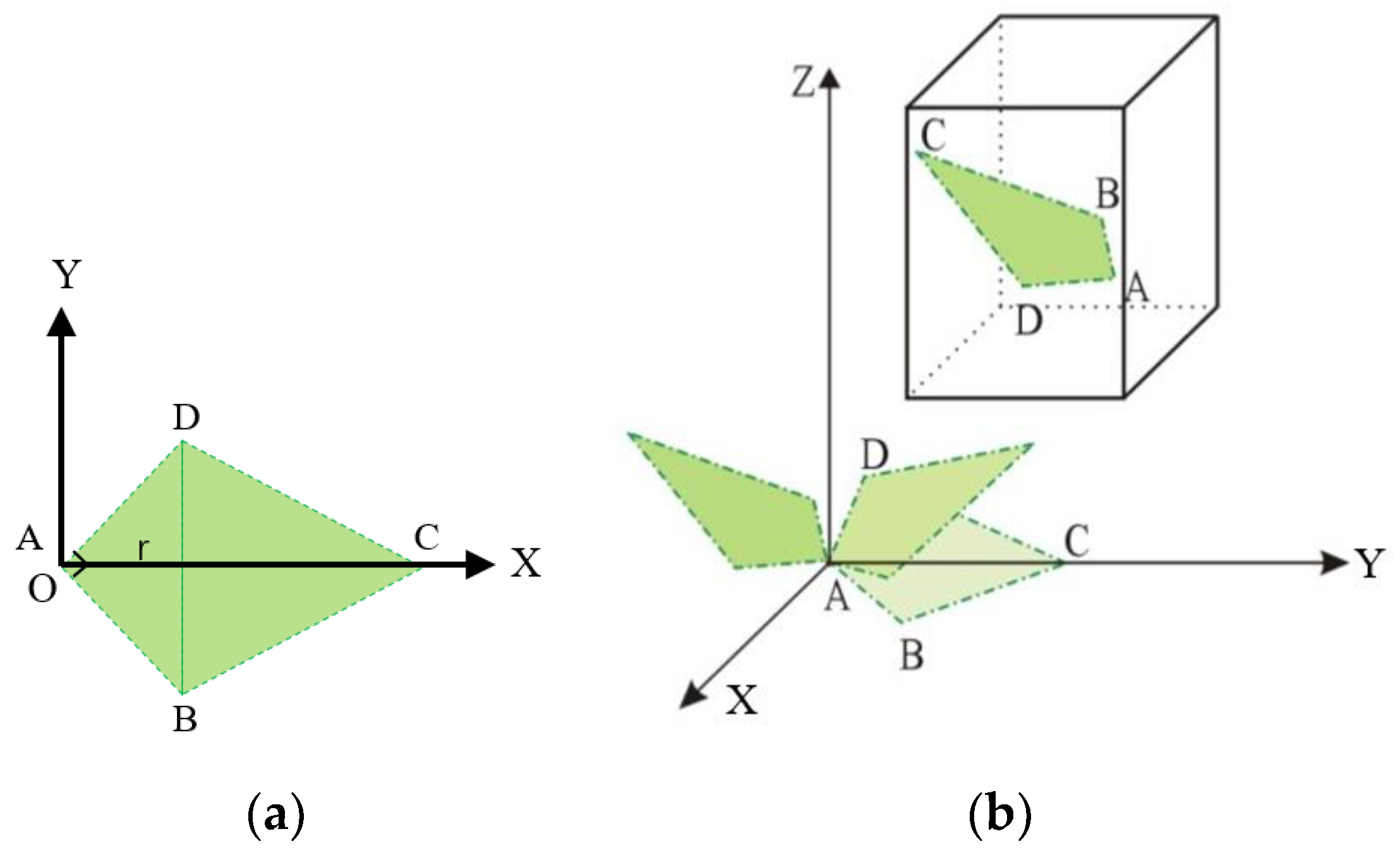
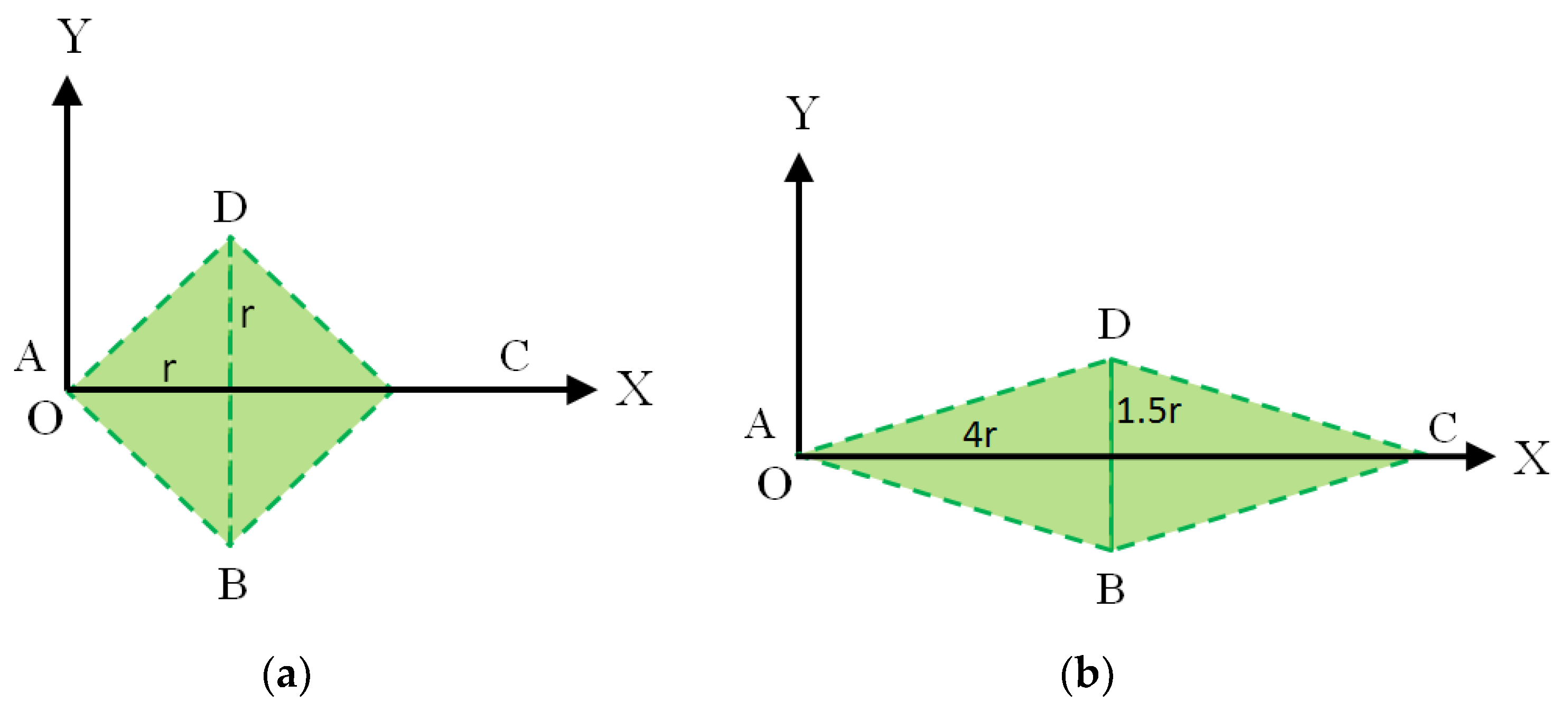
A leaf is simplified to a quadrilateral, which is composed of a right triangle and an equilateral triangle. It is set based on the ratio of the length and width of a clipped leaf measured in the field (Figure 2a). This kind of leaf shape is also used by the generated virtual tree in this study. Its initial four vertex coordinates in the plane of XOY can be expressed as a four-order matrix P [37], with a normal N(0, 0, 1).
The lowest row represents homogeneous term in order to be convenient to transfer this polygon leaf in the space. In Equation (1), r is a leaf shape parameter that controls the size of a leaf. The area of a leaf can be calculated as
3.2.2. Cell division and Leaf Placement
Segmenting the canopy into cubic volumes/voxels based on point clouds can provide a convenient mean of describing the spatial distribution of foliage area in the tree crown [38] and of estimating the leaf area density [21], LAI and LAD [20], etc. Béland et al. [38] investigated the optimal voxel dimensions for estimating the spatial distribution of leaf area density within the crown. They found that the optimal voxel size is a function of leaf size, branching structure, and the predominance of occlusion effects, which provides important guiding principles for the use of voxel volume in the segmentation of point clouds.
In accordance with the research of Béland et al. [38], voxel size is set to 10 cm in this case, which is based on the averaged LA of each tree (Table 1) and branching structure is measured in the field. Assuming that the spatial distribution of leaf areas agrees with the aligned point-cloud density, each leaf point in the crown corresponds to a finite area of leaf , where NUM is the number of total leaf points. Therefore, based on the number of points in each voxel (numi), the area of one leaf in the voxel can be determined using . If the leaf area in the voxel LAi is larger than the maximum leaf area (20 cm2), it would be separated into a standard leaf with an area of 12 cm2 and a smaller leaf. The leaf shape parameter for each leaf, r, can be calculated using:
where LAi is the leaf area in the voxel or the leaf area after division.
Leaf orientation in the voxel is also an important structural parameter. Generally, LAD can be measured in the field or estimated from point clouds using voxels [21]. To simply the procedure of the reconstruction and decrease the needed parameters, an averaged normal direction of all the leaf points in the voxel is used as the normal direction of the added leaf. Where the normal direction for each point is calculated based on the spatial distribution of neighbor points using the CloudCompare software (http://www.danielgm.net/cc/release/).
Leaves are placed in the appropriate cube by rotation and translation, according to their orientation and size. After the process of adding leaves is applied to all of the voxels in the scene, 3D trees with leaves are reconstructed.
3.3. Assemble 3D Scene
All single trees and terrain are reconstructed and assembled. In order to match the locations of the reconstructed trees with the real ones, the reconstructed trees are projected onto the plane to obtain the outlines of trees, and the aligned point clouds are used to outline the four trees (Figure 1). Then, the outlines from the reconstructed trees can be registered with the outlines from the real trees. In this study, the flat terrain is applied. Therefore, all reconstructed trees can be translated in the correct position of the terrain directly, and then the 3D scene is completed.
4. Results and Discussion
4.1. Reconstruction of 3D Scene
4.1.1. Real Scene of the Study Area
The 3D scene of the study area is composed of four single trees and flat ground. In consideration of the effect of occlusion between crowns, only three groups of points for each tree are used to reconstruct each single tree. First, the three sites scans for each tree in Table 1 are aligned, and then the averaged LA for the tree (Table 1) is applied to add leaves and to reconstruct the tree. At last, 3D scene that is similar to the real one is assembled by combining the reconstructed trees on a flat terrain.
4.1.2. Virtual Tree
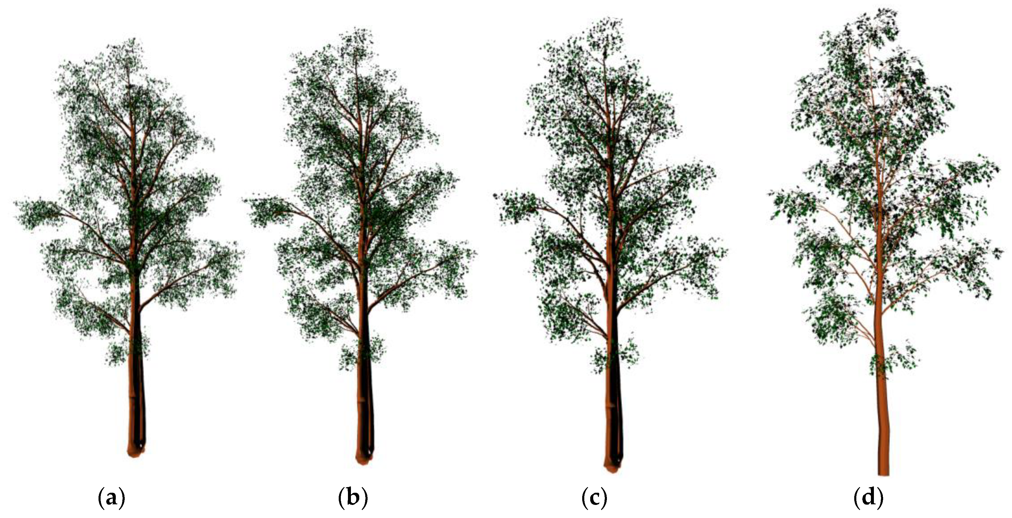
A 3D tree is reconstructed based on the simulated points (Figure 4c). Its leaf area is 20.50 m2 and the relative error of the leaf areas between the reconstructed and the original virtual tree is less than 0.9%. It looks similar to the original tree, including the spatial distribution of leaves.
4.2. Validation
Quantitative validation of the structural characteristics of a rebuilt scene is not a trivial task [27]. The reconstructed scene should not only represent a good visual effect, but it must be structurally consistent with the real canopy. The directional gap fraction is used as an important standard to quantitatively evaluate the geometric accuracy of reconstructed 3D scenes or the 3D structures of trees.
4.2.1. Validation with the Real Scene
Point clouds are simulated based on the reconstructed 3D scene using the ray tracing algorithm [36]. The parameters are set according to the configuration in the field, including scanning position, scanning steps, beam diversity, etc. The measured and simulated point clouds are compared and are shown in Figure 5. It can be seen that they have good similarities in color and structure (the same color represents the same distance).
The directional gap fraction with a zenith angle slices can be expressed as the ratio of the number of laser beams sent into the slice and the number of intercepted laser beams . The sending number is dependent on both the azimuth and zenith range in each slice, as well as the scanning step, and so the intercepted number can be calculated by counting the number of TLS points [40]. Therefore, the gap fraction can be expressed as follows:
where N is the number of the zenith slices, and θ is a middle zenith direction of the layer.
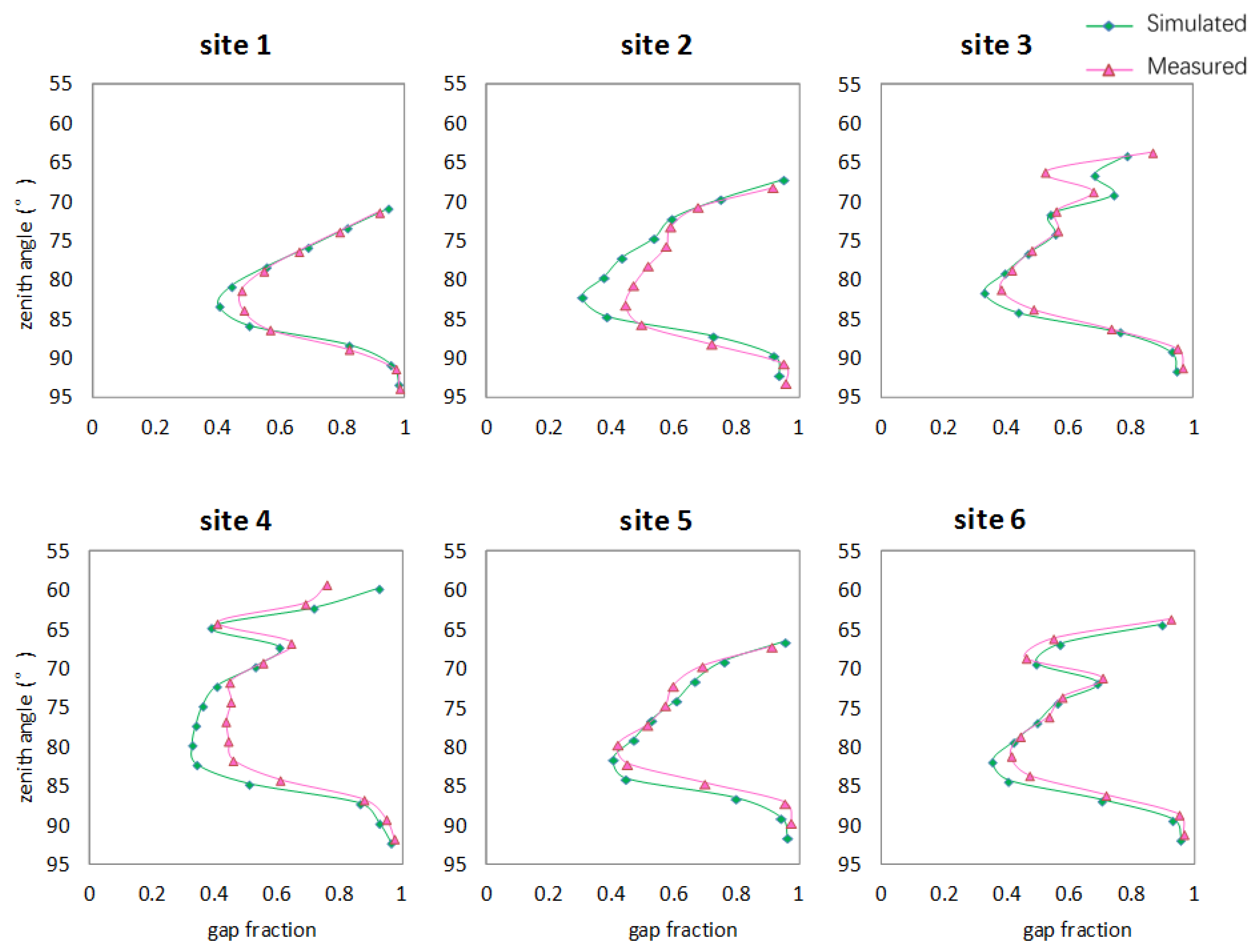
The directional gap fractions for six-site point clouds are calculated based on the measured and simulated data, respectively, and compared in Figure 6. The two groups of directional gap fractions have similar tendencies: they are large in the upper and lower parts and small in the middle, which agree well with the characteristics of the vertical distribution of foliage in the crown. Because the distribution of branches and leaves are not uniform in all crowns, the gap fractions in some directions increase suddenly, such as at 70° for site 3 and 4, and at 75° for site 6 (Figure 6).
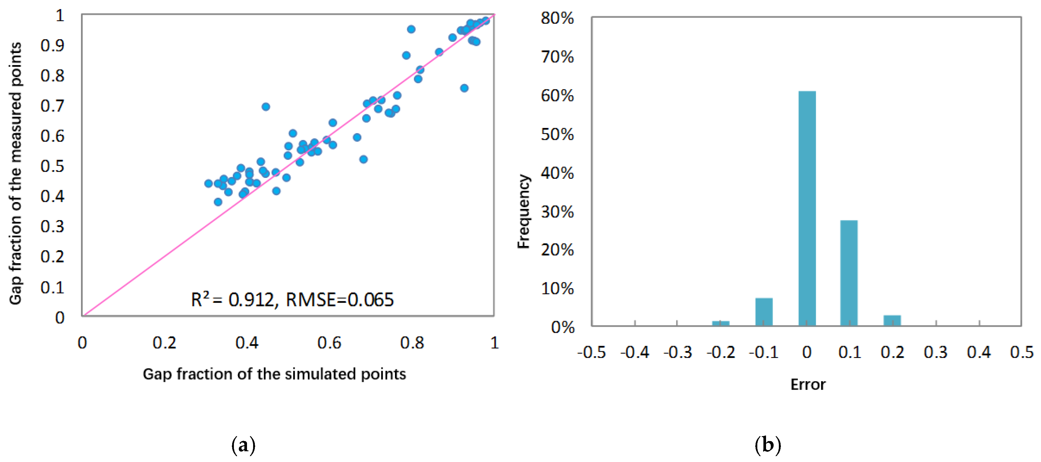
In general, all of the directional gap fractions from the reconstructed scene are in good agreement with those from the real one (Figure 7a). A high correlation coefficient (R2 = 0.912) and a low root mean square error (RMSE = 0.065) between the directional gap fractions that were calculated based on the simulated and measured points quantitatively prove that the method is valid for reconstructing structurally coherent 3D trees.
Although the directional gap fraction is a popular standard to assess the canopy structure, it is affected by the parameters, such as azimuth ranges. It can be seen that there are still a little discrepancies of gap fractions between real and reconstructed trees, as shown in Figure 5. We found that the reason is from the difference of the scanning azimuth ranges in the same slices detected from the simulated and measured points. Generally, the voxel nearby the edge of the crown can reach out of its range, and the added leaves in these voxels often be placed in the centers of the voxels, so that the reconstructed crown is often a little wider than the real one. Accordingly, the azimuthal range of point clouds simulated based on the reconstructed tree is often bigger than the real one. To eliminate the influence of edge effect on the emitted beam numbers, the slicing point density is used to evaluate the structural accuracy of a reconstructed scene.
The slicing point density (PD) with the height is calculated based on all of the aligned points [41].
Here, numi is the number of points in the ith layer with height [Hi, Hi + ΔH]; ΔH is the height interval; and, NUM is the total number of points intercepted by the tree.
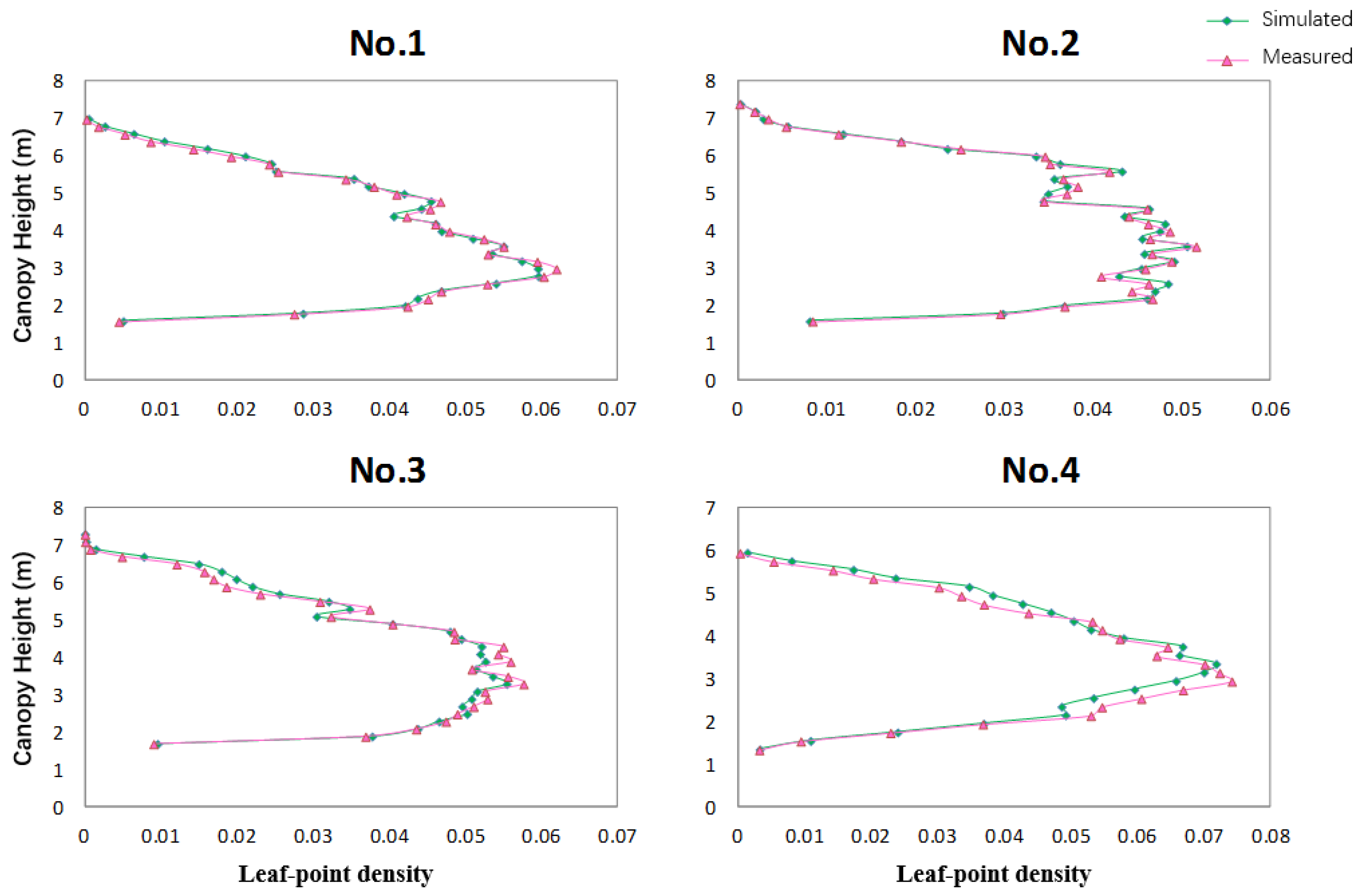
In this study, we pay more attention to the effect of the reconstructed leaf, so the leaf-point density in each slice is calculated based on the separated leaf points. The horizontally slicing leaf-point densities based on the measured and simulated data are compared in Figure 8, and the vertical distribution of leaf-point densities from all four trees agree well.
4.2.2. Validation with the Virtual Tree
Because the 3D virtual tree in Figure 4c is reconstructed based on the simulated points, to improve the reliability of validation, we do not compare the gap fraction or point density calculated with the simulated points from the virtual tree and the reconstructed tree. In this study, some black-and-white images are simulated based on the original and reconstructed trees. These images are built by parallel projecting all triangle facets of the original or reconstructed tree along one view direction to a white plane with a high resolution. The pixel covered by the projected facet (>50%) is black. Then, a gap fraction can be calculated from this image using the pixel ratio (a ratio of the white pixel numbers to the total number of pixels in the image).
The black-and-white images are simulated from several directions, including eight azimuth angles (0°, 45°, 90°, 135°, 180°, 225°, 270°, 315°) and five zenith angles (45°, 63°, 76°, 90°, 162°). Images with the zenith directions of (45°, 63°, 76°, 90°) are projected from bottom to top, and the image with 162° zenith direction is projected from top to bottom. Then, the relative error of the directional gap fractions obtained using the simulated images from the original and reconstructed trees are shown in Figure 9. The relative errors of the directional gap fractions are not more than 4.1%, which strongly supports the feasibility of our reconstruction method. The relative errors for different azimuth directions have no apparent difference because the structure of the generated virtual tree is basically azimuthally symmetrical.
5. Discussion
5.1. Completeness and Accuracy of the Reconstructed Tree
By applying our method to a real scene and a virtual tree, the reconstructed results show pretty well visual effects. However, after quantitatively comparing the directional gap fractions and point densities of the original and reconstructed ones, it is found that the occlusion and density distribution of points will affect the completeness and accuracy of the reconstructed tree.
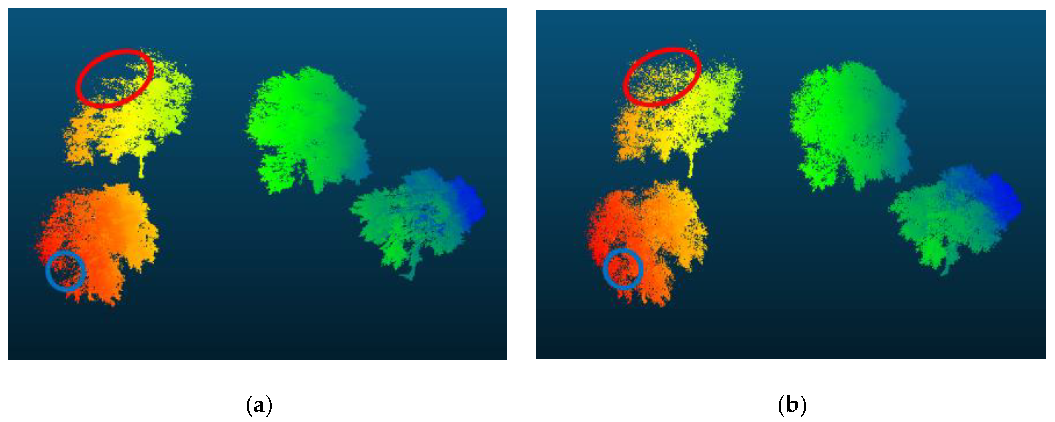
As is known to all, the occlusion issue is inevitable for TLS to scan canopies. Although aligned multi-site scanned points can partly cover the shortage, the issue still cannot be solved completely for some dense crowns. For example, there are some small differences in Figure 5, highlighted using circles. One reason is that the scanner positions that were used in the simulation do not coincide with the one in the field. Therefore, some points occluded in the measured data (circle in Figure 5a) can be scanned in the simulation ones (Figure 5b).
Additionally, it can be seen from Figure 9 that the directional gap fractions are underestimated in the bottom-to-top zenith directions (45°, 63°, 76°, 90°), but overestimated in the top-to-bottom zenith direction (162°). The major reason for this difference is the effect of point cloud occlusion. Because the TLS device is often used on the ground with a bottom-to-up scanning style, the upper crowns are inevitably occluded and only a few points from the upper parts of the tree can be obtained. Another reason is that the point density distribution is not uniform: the point density is larger in the lower part of the tree but is smaller than normal in the upper part of the tree. Because the tree reconstruction depends entirely on the spatial distribution of points, more leaves are added to the lower crown. This means that the relative errors for directional gap fractions that are close to the vertical directions (such as 45° and 162°, in this case) will be enlarged.
5.2. Sensitivity of the Leaf Shape
The leaf shape is various in the real world. It can be represented as some simple shapes. In this study, we use a quadrilateral, simplified based on the measured structure to reconstruct the trees. Similarly, the leaf can also be simplified as other shapes, such as a square or a rhombus (Figure 10). Then, the initial four vertex coordinates can be expressed as
The leaf area can be calculated as
Then, the leaf shape parameter, r, can be obtained by and .
The virtual trees (Figure 4a) are reconstructed using the new leaf shapes, respectively (Figure 11). All reconstructed trees with different leaf shapes look similar.
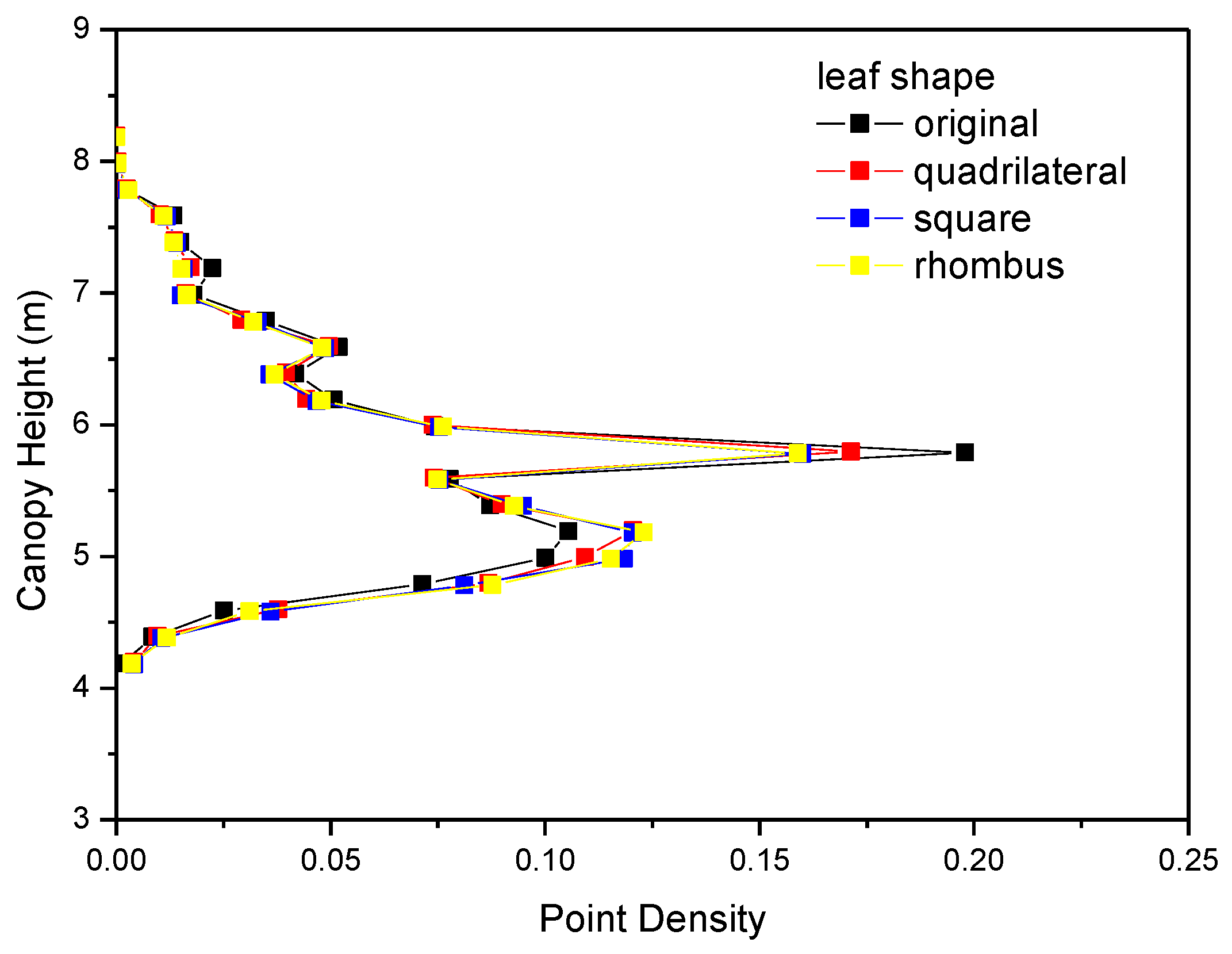
Then point clouds of these three reconstructed virtual trees (Figure 11a–c) are simulated based on the same parameters (the sensor height, scanning distance and step). The slicing point density of each set of point clouds is calculated and compared in Figure 12.
These point densities agree well with the original ones. Specially, the point densities from the reconstructed trees are closer than that from the original virtual tree. RMSEs of the vertical point densities between the reconstructed trees and the original one are 1.10% (square leaf shape), 1.13% (rhombus leaf shape), and 0.88% (quadrilateral leaf shape), separately. The reconstructed tree with the typical leaf shape (quadrilateral) shows better similarity with the original one. When comparing within these reconstructed trees, RMSEs of the point densities are no more than 0.4%. It means that the reconstructed trees are more similar to each other.
Overall, our method is not sensitive to the leaf shape.
6. Conclusions
Based on TLS point cloud data, we developed the method for reconstructing entire 3D trees in this study. This method can effectively add leaves that are based on voxels and is insensitive to the leaf shape. Its performance is evaluated over a reconstructed small 3D scene and a virtual tree using the directional gap fraction and point density distribution, and it shows good consistency in leaf area and directional gap fraction of crowns when compared with the point cloud from the original ones. The relative errors of the gap fractions (the virtual tree) are less than 4.1%.
While analyzing the directional gap fraction that is based on a virtual 3D tree, it is found that the reconstructed 3D trees are influenced by the effect of point cloud occlusion because the method is completely dependent on the spatial distribution of points. Though this method may slightly underestimate the leaf area for the upper crowns, and overestimate for the lower crowns, it is still feasible and has the potential to contribute the quantitative remote sensing in canopy radiative transfer models.
Several factors that impact the reconstruction of trees and some future possible improvements are summarized, including the quality of point clouds, the point classification, and LA retrieval accuracy. First, the quality of point clouds is critical, and factors, such as occlusion and ghost points, greatly complicate the data preprocessing and decrease the structural accuracy of reconstructed trees. In the future, it will be necessary to study how TLS data can be combined with supplementary data (such as ALS-aircraft laser scanner data or UAV data) to reconstruct 3D trees and reduce the effect of occlusions. Another option would be to apply the growing rules of plants to overcome the disadvantages of point clouds. Second, point classification accuracy is dependent of the quality of photographs, the classification algorithm and the registration between points and photographs. Bad classification results not only affect the LA retrieval, but also decrease the accuracy of reconstructed branches and leaves. Dual-wavelength [43] or multiple spectra laser sensors can help to improve the classification accuracy and to simplify the classifying process. Third, the LA of a real tree is determined using a retrieved value, and its accuracy will directly affect the reconstructed tree structure. Therefore, it is necessary to improve the retrieval algorithm for LA in the future.
In summary, the method that is presented for reconstructing 3D trees shows its potential in reconstructing complex forest scene and in evaluating the parameters of land surface ecosystem.
Author Contributions
Donghui Xie and Xiangyu Wang developed the method of reconstructing 3D trees; Jianbo Qi simulated point cloud data; Yiming Chen, Xihan Mu, Wuming Zhang and Guangjian Yan designed and performed the experiment; Yiming Chen help process the point clouds and all authors contributed in writing the paper.
Acknowledgments
This work is supported by National Natural Science Foundation of China (Grant No. 41571341, 41331171). Thanks the colleagues who helped collect field data and its processing.
Conflicts of Interest
The authors declare no conflict of interest.
References
- Morsdorf, F.; Meier, E.; Kötz, B.; Itten, K.I.; Dobbertin, M.; Allgöwer, B. LIDAR-based geometric reconstruction of boreal type forest stands at single tree level for forest and wildland fire management. Remote Sens. Environ. 2004, 92, 353–362. [Google Scholar] [CrossRef]
- Seidl, R.; Rammer, W.; Scheller, R.M.; Spies, T.A. An individual-based process model to simulate landscape-scale forest ecosystem dynamics. Ecol. Model. 2012, 231, 87–100. [Google Scholar] [CrossRef]
- Disney, M.; Lewis, P.; Saich, P. 3D modelling of forest canopy structure for remote sensing simulations in the optical and microwave domains. Remote Sens. Environ. 2006, 100, 114–132. [Google Scholar] [CrossRef]
- Fleck, S.; van der Zande, D.; Schmidt, M.; Coppin, P. Reconstructions of tree structure from laser-scans and their use to predict physiological properties and processes in canopies. Int. Arch. Photogramm. Remote Sens. Spat. Inf. Sci. 2004, 36, 119–123. [Google Scholar]
- Verhoef, W. Light scattering by leaf layers with application to canopy reflectance modeling: The SAIL model. Remote Sens. Environ. 1984, 16, 125–141. [Google Scholar] [CrossRef]
- Suits, G.H. The calculation of the directional reflectance of a vegetative canopy. Remote Sens. Environ. 1973, 2, 117–125. [Google Scholar] [CrossRef]
- Kubelka, P.; Munk, F. Ein beitrag zur optik der farbanstriche. Zeitschrift fur Technische Physik 1931, 12, 501–593. [Google Scholar]
- Li, X.; Strahler, A.H. Geometric-optical modeling of a conifer forest canopy. IEEE Trans. Geosci. Remote Sens. 1985, 5, 705–721. [Google Scholar] [CrossRef]
- Li, X.; Strahler, A.H. Geometric-optical bidirectional reflectance modeling of the discrete crown vegetation canopy: Effect of crown shape and mutual shadowing. IEEE Trans. Geosci. Remote Sens. 1992, 30, 276–292. [Google Scholar] [CrossRef]
- Chen, J.M.; Leblanc, S.G. A four-scale bidirectional reflectance model based on canopy architecture. IEEE Trans. Geosci. Remote Sens. 1997, 35, 1316–1337. [Google Scholar] [CrossRef]
- España, M.L.; Baret, F.; Aries, F.; Chelle, M.; Andrieu, B.; Prévot, L. Modeling maize canopy 3D architecture: Application to reflectance simulation. Ecol. Model. 1999, 122, 25–43. [Google Scholar] [CrossRef]
- Goel, N.S.; Qin, W. Influences of canopy architecture on relationships between various vegetation indices and LAI and FPAR: A computer simulation. Remote Sens. Rev. 1994, 10, 309–347. [Google Scholar] [CrossRef]
- Goel, N.S.; Rozehnal, I.; Thompson, R.L. A computer graphics based model for scattering from objects of arbitrary shapes in the optical region. Remote Sens. Environ. 1991, 36, 73–104. [Google Scholar] [CrossRef]
- Govaerts, Y.M.; Verstraete, M.M. Raytran: A Monte Carlo ray-tracing model to compute light scattering in three-dimensional heterogeneous media. IEEE Trans. Geosci. Remote Sens. 1998, 36, 493–505. [Google Scholar] [CrossRef]
- Qin, W.; Gerstl, S.A. 3-D scene modeling of semidesert vegetation cover and its radiation regime. Remote Sens. Environ. 2000, 74, 145–162. [Google Scholar] [CrossRef]
- Gastellu-Etchegorry, J.-P.; Demarez, V.; Pinel, V.; Zagolski, F. Modeling radiative transfer in heterogeneous 3-D vegetation canopies. Remote Sens. Environ. 1996, 58, 131–156. [Google Scholar] [CrossRef]
- Huang, H.; Qin, W.; Liu, Q. RAPID: A Radiosity Applicable to Porous IndiviDual Objects for directional reflectance over complex vegetated scenes. Remote Sens. Environ. 2013, 132, 221–237. [Google Scholar] [CrossRef]
- Disney, M.; Lewis, P.; North, P. Monte Carlo ray tracing in optical canopy reflectance modelling. Remote Sens. Rev. 2000, 18, 163–196. [Google Scholar] [CrossRef]
- Widlowski, J.-L.; Côté, J.-F.; Béland, M. Abstract tree crowns in 3D radiative transfer models: Impact on simulated open-canopy reflectances. Remote Sens. Environ. 2014, 142, 155–175. [Google Scholar] [CrossRef]
- Zheng, G.; Moskal, L.M. Leaf orientation retrieval from terrestrial laser scanning (TLS) data. IEEE Trans. Geosci. Remote Sens. 2012, 50, 3970–3979. [Google Scholar] [CrossRef]
- Hosoi, F.; Nakai, Y.; Omasa, K. 3-D voxel-based solid modeling of a broad-leaved tree for accurate volume estimation using portable scanning lidar. ISPRS J. Photogramm. Remote Sens. 2013, 82, 41–48. [Google Scholar] [CrossRef]
- Bucksch, A.; Lindenbergh, R.C.; Menenti, M. Skeltre-fast skeletonisation for imperfect point cloud data of botanic trees. In Proceedings of the 2nd Eurographics Conference on 3D Object Retrieval, Eurographics, Munich, Germany, 29 March–3 April 2009; pp. 13–20. [Google Scholar]
- Livny, Y.; Yan, F.; Olson, M.; Chen, B.; Zhang, H. Automatic reconstruction of tree skeletal structures from point clouds. In Proceedings of the ACM Transactions on Graphics (TOG), Seoul, Korea, 15–18 December 2010. [Google Scholar]
- Wang, Z.; Zhang, L.; Fang, T.; Mathiopoulos, P.T.; Qu, H.; Chen, D.; Wang, Y. A structure-aware global optimization method for reconstructing 3-D tree models from terrestrial laser scanning data. IEEE Trans. Geosci. Remote Sens. 2014, 52, 5653–5669. [Google Scholar] [CrossRef]
- Huang, H.; Chen, C.; Zou, J.; Lin, D. Tree geometrical 3D modeling from terrestrial laser scanned point clouds: A review. Sci. Silvae Sin. 2013, 49, 123–130. [Google Scholar]
- Xu, H.; Gossett, N.; Chen, B. Knowledge and heuristic-based modeling of laser-scanned trees. ACM Trans. Graph. 2007, 26, 19. [Google Scholar] [CrossRef]
- Côté, J.-F.; Widlowski, J.L.; Fournie, R.A.; Verstraete, M.M. The structural and radiative consistency of three-dimensional tree reconstructions from terrestrial Lidar. Remote Sens. Environ. 2009, 113, 1067–1081. [Google Scholar] [CrossRef]
- Tao, S.; Guo, Q.; Xu, S.; Su, Y.; Li, Y.; Wu, F. A geometric method for wood-leaf separation using terrestrial and simulated Lidar data. Photogramm. Eng. Remote Sens. 2015, 81, 767–776. [Google Scholar] [CrossRef]
- Reymann, C.; Lacroix, S. Improving LiDAR point cloud classification using intensities and multiple echoes. In Proceedings of the 2015 IEEE/RSJ International Conference on Intelligent Robots and Systems (IROS), Hamburg, Germany, 28 September–2 October 2015; pp. 5122–5128. [Google Scholar]
- Zhu, Z.; Zhang, W.; Zhu, L.; Zhao, J. Research on different slicing methods of acquiring LAI from terrestrial laser scanner data. In Proceedings of the 2011 IEEE International Conference on Spatial Data Mining and Geographical Knowledge Services (ICSDM), Fuzhou, China, 29 June–1 July 2011; pp. 295–299. [Google Scholar]
- Zhang, W.; Zhao, J.; Chen, M.; Chen, Y.; Yan, K.; Li, L.; Qi, J.; Wang, X.; Luo, J.; Chu, Q. Registration of optical imagery and LiDAR data using an inherent geometrical constraint. Opt. Express 2015, 23, 7694–7702. [Google Scholar] [CrossRef] [PubMed]
- Axelsson, P. DEM generation from laser scanner data using adaptive TIN models. Int. Arch. Photogramm. Remote Sens. 2000, 33, 111–118. [Google Scholar]
- Zhang, W.; Qi, J.; Wan, P.; Wang, H.; Xie, D.; Wang, X.; Yan, G. An easy-to-use airborne LiDAR data filtering method based on cloth simulation. Remote Sens. 2016, 8, 501. [Google Scholar] [CrossRef]
- Xie, D.; Wang, Y.; Hu, R.; Chen, Y.; Yan, G.; Zhang, W.; Wang, P. A modified gap fraction model of individual trees for estimating leaf area index using terrestrial laser scanner. J. Appl. Remote Sens. 2017, 11, 035012. [Google Scholar] [CrossRef]
- Disney, M.I.; Lewis, P.E.; Bouvet, M.; Prieto-Blanco, A.; Hancock, S. Quantifying surface reflectivity for spaceborne LiDAR via two independent methods. IEEE Trans. Geosci. Remote Sens. 2009, 47, 3262–3271. [Google Scholar] [CrossRef]
- Wang, Y. Simulation and analysis of point clouds from a terrestrial laser scanner. J. Remote Sens. 2015, 19, 391–399. [Google Scholar]
- Donald, H.; Pauline, B.; Warren, R. Computer Graphics with OpenGL, 4th ed.; Prentice Hall PTR: Upper Saddle River, NJ, USA, 2010. [Google Scholar]
- Béland, M.; Baldocchi, D.D.; Widlowski, J.L.; Fournier, R.A.; Verstraete, M.M. On seeing the wood from the leaves and the role of voxel size in determining leaf area distribution of forests with terrestrial LiDAR. Agric. For. Meteorol. 2014, 184, 82–97. [Google Scholar] [CrossRef]
- Matt, P.; Wenzel, J.; Greg, H. Physically Based Rendering: From Theory to Implementation; Elsevier Science & Technology Publication: San Francisco, CA, USA, 2016. [Google Scholar]
- Danson, F.M.; Hetherington, D.; Morsdorf, F.; Koetz, B.; Allgower, B. Forest canopy gap fraction from terrestrial laser scanning. IEEE Trans. Geosci. Remote Sens. 2007, 4, 157–160. [Google Scholar] [CrossRef] [Green Version]
- Zhu, Z.; Zhang, W. Estimating the LAI of a single tree from terrestrial laser scanner data. In Proceedings of the 2011 IEEE International Conference on Remote Sensing, Environment and Transportation Engineering (RSETE), Nanjing, China, 24–26 June 2011; pp. 4947–4951. [Google Scholar]
- Paris, C.; Kelbe, D.; van Aardt, J.; Bruzzone, L. A novel automatic method for the fusion of ALS and TLS LiDAR data for robust assessment of tree crown structure. IEEE Trans. Geosci. Remote Sens. 2017, 55, 3679–3693. [Google Scholar] [CrossRef]
- Douglas, E.S.; Strahler, A.; Martel, J.; Cook, T.; Mendillo, C.; Marshall, R.; Chakraba, S.; Woodcock, C.; Li, Z.; Yang, X.; et al. DWEL: A dual-wavelength echidna lidar for ground-based forest scanning. In Proceedings of the 2012 IEEE International Geoscience and Remote Sensing Symposium (IGARSS 2012), Munich, Germany, 22–27 July 2012; pp. 4998–5001. [Google Scholar]
Figure 1.
Relative positions of the four trees (No. 1, 2, 3, and 4) and six scanning sites (orange points), as seen from above. The outlines of the trees were drawn by projecting the scanned points in nadir.
Figure 1.
Relative positions of the four trees (No. 1, 2, 3, and 4) and six scanning sites (orange points), as seen from above. The outlines of the trees were drawn by projecting the scanned points in nadir.

Figure 2.
Diagram of leaf geometry (a) and its transform (b).

Figure 3.
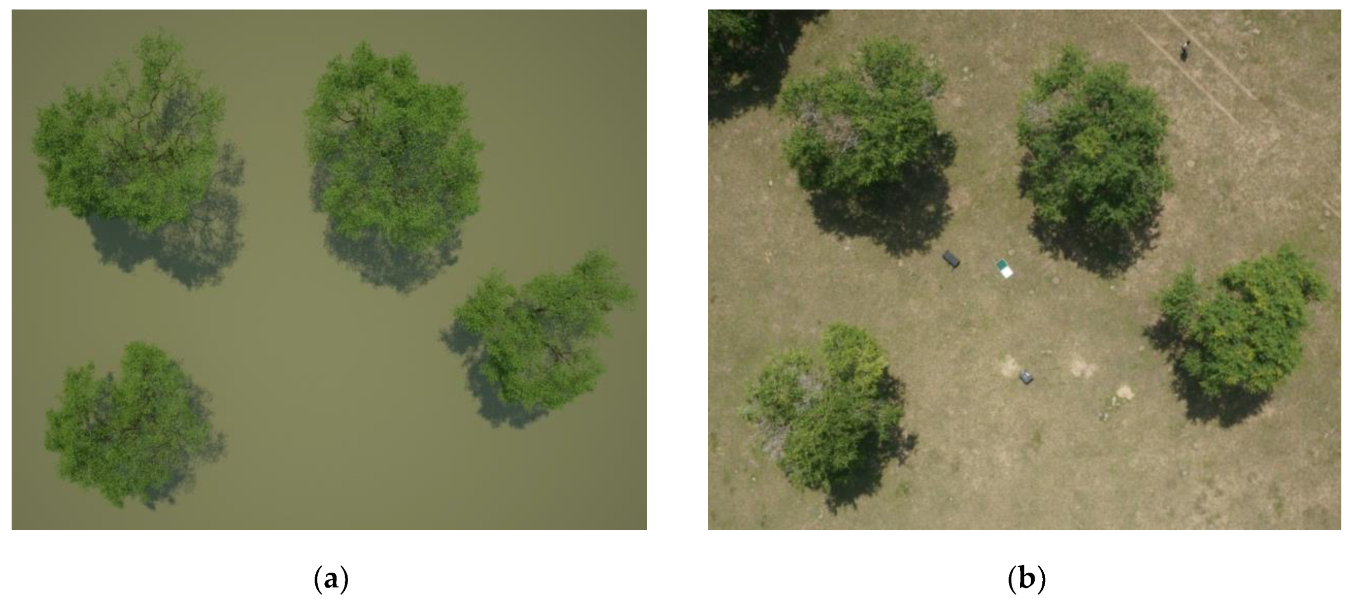
Comparison of simulated and real photos: (a) Simulated photograph based on the reconstructed scene; and, (b) Real photograph taken from unmanned aerial vehicle (UAV).
Figure 3.
Comparison of simulated and real photos: (a) Simulated photograph based on the reconstructed scene; and, (b) Real photograph taken from unmanned aerial vehicle (UAV).

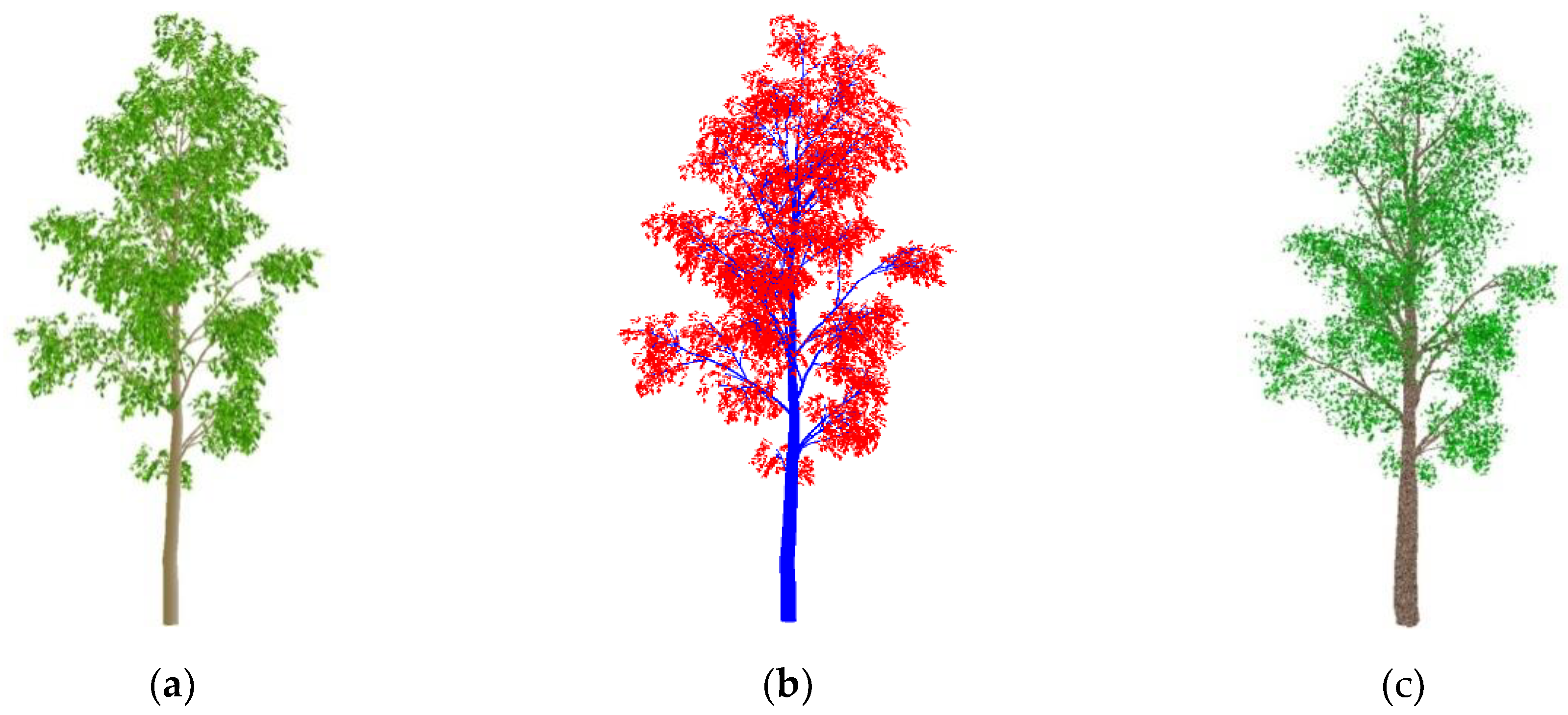
Figure 4.
(a) A virtual tree generated with OnyxTREE software; (b) The simulated point clouds based on the virtual tree (Blue points represent trunks/branches and red points represent leaves); and, (c) The reconstructed 3D tree.
Figure 4.
(a) A virtual tree generated with OnyxTREE software; (b) The simulated point clouds based on the virtual tree (Blue points represent trunks/branches and red points represent leaves); and, (c) The reconstructed 3D tree.

Figure 5.
Comparison of the measured (a) and simulated (b) point clouds for one scan. The different colors represent the distances from scanner to objects. The red and blue circles highlight the difference between the measured and simulated point clouds.
Figure 5.
Comparison of the measured (a) and simulated (b) point clouds for one scan. The different colors represent the distances from scanner to objects. The red and blue circles highlight the difference between the measured and simulated point clouds.

Figure 6.
Comparison of the directional gap fractions from measured and simulated points for each site scan (zenith angle interval: 2.5°).
Figure 6.
Comparison of the directional gap fractions from measured and simulated points for each site scan (zenith angle interval: 2.5°).

Figure 7.
Relationship between the directional gap fractions of measured and simulated points (a) and the distribution of their errors (b).
Figure 7.
Relationship between the directional gap fractions of measured and simulated points (a) and the distribution of their errors (b).

Figure 8.
Comparison of the sliced leaf-point densities for each tree (No. 1–4), calculated based on measured and simulated point clouds (interval height: 0.2 m).
Figure 8.
Comparison of the sliced leaf-point densities for each tree (No. 1–4), calculated based on measured and simulated point clouds (interval height: 0.2 m).

Figure 9.
Relative errors of the gap fractions from the black-and-white images with different view directions simulated based on the original virtual tree and the reconstructed one.
Figure 9.
Relative errors of the gap fractions from the black-and-white images with different view directions simulated based on the original virtual tree and the reconstructed one.

Figure 10.
Diagram of leaf shape: (a) Square, (b) Rhombus.

Figure 11.
Comparison of the reconstructed trees using the different leaf shapes, including (a) rhombus, (b) square and (c) typical quadrilateral, with (d) the original virtual tree.
Figure 11.
Comparison of the reconstructed trees using the different leaf shapes, including (a) rhombus, (b) square and (c) typical quadrilateral, with (d) the original virtual tree.

Figure 12.
Comparison of point densities based on the simulated point clouds of the reconstructed trees with different leaf shapes and the original virtual tree (interval height: 0.2m).
Figure 12.
Comparison of point densities based on the simulated point clouds of the reconstructed trees with different leaf shapes and the original virtual tree (interval height: 0.2m).


Table 1.
The retrieval leaf areas and scanner sites for each tree.
| Tree ID | Averaged LA (m2) | Site ID | Retrieval LA (m2) |
|---|---|---|---|
| No.1 | 71.236 | Site 1 | 71.910 |
| Site 3 | 71.350 | ||
| Site 6 | 70.449 | ||
| No.2 | 75.895 | Site 1 | 80.548 |
| Site 4 | 80.663 | ||
| Site 5 | 66.474 | ||
| No.3 | 65.546 | Site 1 | 62.394 |
| Site 2 | 71.946 | ||
| Site 4 | 64.298 | ||
| No.4 | 48.075 | Site 1 | 47.825 |
| Site 2 | 49.041 | ||
| Site 5 | 47.359 |
© 2018 by the authors. Licensee MDPI, Basel, Switzerland. This article is an open access article distributed under the terms and conditions of the Creative Commons Attribution (CC BY) license (http://creativecommons.org/licenses/by/4.0/).
Share and Cite
MDPI and ACS Style
Xie, D.; Wang, X.; Qi, J.; Chen, Y.; Mu, X.; Zhang, W.; Yan, G. Reconstruction of Single Tree with Leaves Based on Terrestrial LiDAR Point Cloud Data. Remote Sens. 2018, 10, 686. https://doi.org/10.3390/rs10050686
AMA Style
Xie D, Wang X, Qi J, Chen Y, Mu X, Zhang W, Yan G. Reconstruction of Single Tree with Leaves Based on Terrestrial LiDAR Point Cloud Data. Remote Sensing. 2018; 10(5):686. https://doi.org/10.3390/rs10050686
Chicago/Turabian StyleXie, Donghui, Xiangyu Wang, Jianbo Qi, Yiming Chen, Xihan Mu, Wuming Zhang, and Guangjian Yan. 2018. "Reconstruction of Single Tree with Leaves Based on Terrestrial LiDAR Point Cloud Data" Remote Sensing 10, no. 5: 686. https://doi.org/10.3390/rs10050686
Note that from the first issue of 2016, this journal uses article numbers instead of page numbers. See further details here.