Optimizing Window Length for Turbulent Heat Flux Calculations from Airborne Eddy Covariance Measurements under Near Neutral to Unstable Atmospheric Stability Conditions

Abstract

Airborne eddy covariance (EC) is one of the most effective ways to directly measure turbulent flux at a regional scale. This study aims to find the optimum spatial window length for turbulent heat fluxes calculation from airborne eddy covariance measurements under near neutral to unstable atmospheric stability conditions, to reduce the negative influences from mesoscale turbulence, and to estimate local meaningful turbulent heat fluxes accurately. The airborne flux measurements collected in 2008 in the Netherlands were used in this study. Firstly, the raw data was preprocessed, including de-spike, segmentation, and stationarity test. The atmospheric stability conditions were classified as near neutral, moderately unstable, or very unstable; the stable condition was excluded. Secondly, Ogive analysis for turbulent heat fluxes from all available segmentations of the airborne measurements was used to determine the possible window length range. After that, the optimum window length for turbulent heat flux calculations was defined based on the analysis of all possible window lengths and their uncertainties. The results show that the choice of the optimum window length strongly depends on the atmospheric stability conditions. Under near neutral conditions, local turbulence is mixed insufficiently and vulnerable to heterogeneous turbulence. A relatively short window length is needed to exclude the influence of mesoscale turbulence, and we found the optimum window length ranges from 2000 m to 2500 m. Under moderately unstable conditions, the typical scale of local turbulence is relative large, and the influence of mesoscale turbulence is relatively small. We found the optimum window length ranges from 3900 m to 5000 m. Under very unstable conditions, large convective eddies dominate the transmission of energy so that the window length needs to cover the large eddies with large energy transmission. We found the optimum window length ranges from 4500 m to 5000 m. This study gives a comprehensive methodology to determine the optimizing window length in order to compromise a balance between the accuracy and the surface representativeness of turbulent heat fluxes from airborne EC measurements.

1. Introduction

Information on the heat and moisture flux exchanges between the land surface and the atmosphere is crucial for a better understanding of the role of terrestrial ecosystems in the global climate system. Reliable land surface flux measurements or estimates, especially at regional scales, are frequently used to constrain or evaluate dynamic earth system models, such as regional climate models, regional hydrological models, and global circulation models [1,2]. The tower-based eddy covariance (EC) method provides turbulent flux measurements with good temporal samples (e.g., every 30 min) but usually with a small spatial representative (i.e., footprint, typically less than 1 km²) [3,4]. Generally, such a small footprint cannot adequately describe the mean surface flux of a grid of the land surface model or a pixel of satellite observations with coarser spatial resolutions if the land surface is heterogeneous. Compared to the tower-based EC measurements of turbulent fluxes, airborne EC technology with a larger footprint (typically more than 10 km²) has more potential to provide turbulent flux measurements with a better spatial coverage [5,6].

As the standardized micrometeorological technique, the EC method measures the transfer of energy and matter between terrestrial ecosystems and the atmosphere by the covariance between turbulent fluctuations of the vertical wind and the quantity of interest [7,8]. The basic assumptions behind the EC method mainly include stationarity, horizontal homogeneity, and fully developed turbulent flow [9,10]. One crucial factor determining the accuracy of EC measurements is the choice of integral time or length interval of the corresponding turbulence, which is strongly connected to the basic assumptions of the EC method [10]. Conventionally, the cospectral analysis method can be used to decompose the flux into frequency- or wavenumber-dependent contributions of turbulence for studying the distribution of turbulent energy among the different turbulence scales. For the EC measurements, turbulent fluxes driven by the high-frequency components of turbulence are inherent in local surface exchange, whereas fluxes driven by the low-frequency components (i.e., mesoscale eddies) possibly result from surface heterogeneity at the landscape scale [11,12,13]. One major technique used to determine the necessary integral interval is the Ogive analysis method, which is defined as the cumulative sum of a cospectral from low to high frequency. If the Ogive curve approaches an asymptote at a low frequency, the point of convergence of the cumulative cospectral is the optimum turbulent flux averaging integral interval. However, the influences of mesoscale turbulence may result in the Ogive curve not converging to an asymptote, and this may make it difficult to determine the integral interval. The optimum choice of the integral interval should ensure that the EC measurements capture all scales of local turbulent transporting, but not be contaminated by mesoscale eddies (nonstationary or heterogeneous), which are independent of the local surface exchange [11,14,15]. In general, a spectral gap of turbulence is assumed to exist between the high- and low-frequency components of turbulence, which allows the users to separate “locally meaningful” fluxes from mesoscale motions of atmospheric turbulence [11,16,17]. If the Ogive curve converges to an asymptote at a frequency over the low-frequency domain, it represents a clear spectral gap. However, the presence of a spectral gap maybe not always be evident, especially for unstable conditions where the strong mixing of turbulence from local patches maybe lead to a blurred distinction between turbulence and mesoscale motion. If a spectral gap appears in the spectrum of turbulence, it will provide useful information about a good choice of the integral interval for turbulent flux determination. If the spectral gap is unclear or absent, other methods such as “ensemble block averaging” or statistical error analysis can also be used to find the integral interval [18,19,20]. However, these methods cannot decompose the turbulent flow, and the decomposition of turbulence is very important for studying the distribution of turbulent energy among the different wavelengths. This paper will show the integration of these methods, which was used to study the optimum integral interval for turbulent flux calculation. For the tower-based EC measurements, the integral interval of flux estimates is expressed as an averaging time, which can be related to a sample length by multiplying the mean wind speed by the averaging time [21]. This could be regarded as a passive measurement method because of the detecting eddies brought by the mean wind [22]. Numerous researchers have carried out studies to determine the optimum averaging periods over different sites, and the results revealed that the traditional 30 min averaging time should be adjusted or site-specific to capture all fluxes taking place on a field scale and to avoid the influence of low-frequency turbulence [10,12,18,23,24].

Airborne EC measurement is an active measurement method, in which an aircraft typically flies an order of magnitude faster than the mean wind speed [21]. Fluxes from airborne EC measurements are areal averages over the measurement footprint along the flight path instead of time [25]. Airborne flux measurements mainly provide the approximate “true” surface flux values at the regional scale, which can be used to calibrate and validate process-oriented models in which land surface fluxes are linked to local surface exchange processes [17,26,27,28]. This study will also focus on this application background. So, the integral interval or averaging length (i.e., window length) of the airborne EC method needs to be long enough to provide an adequate turbulence sample, as well as short enough to resolve the signal from the surface heterogeneity [27,29,30]. However, few studies have addressed how to choose a proper window length to estimate local meaningful fluxes using the airborne EC method. This may be due to the complex relationships between turbulent fluxes and the underlying surface, atmospheric conditions, and measurement height [31]. For airborne EC measurements at the middle or high part of the convective boundary layer, a long window length (typically 10–20 km) is normally required to achieve reliable flux estimates [32,33,34,35]. In theory, Lenschow and Stankov [21] estimated very long window lengths (about 100 km for summer at the middle of the mixing layer over a relatively horizontally homogeneous situation) to achieve 10% measurement accuracy. The measurement error tends to be underestimated by their method due to the assumption of Gaussian distribution for the velocity and scalar variables [36]. These long window lengths are needed because of the size of the turbulence eddies increases with the distance above the ground surface [37]. However, the calculated fluxes based on the long window length lose the ability to resolve the surface heterogeneity, which is very important for land surface exchange investigations [27]. To better describe the surface heterogeneity, it is necessary to perform airborne EC measurements close to the ground (i.e., in the near-surface layer), where characteristic fluxes from different land covers are not yet fully homogenized or blended [6,26,34,38]. For airborne EC measurements in the near-surface layer, a short window length can produce reliable turbulent flux that contains more information about spatial variability. According to Desjardins et al. [38], at the flight level of 25 m above the ground, the turbulent flux values from the window length of 4 km were close to the values calculated with a window length between 12 km and 16 km over a relatively homogeneous surface. Similar results from Vickers and Mahrt [29] indicated that the turbulent flux calculated with a window length of 1.28 km could capture 90% of the turbulent flux from a window length of 16 km at an altitude of 30 m above the ground level over a heterogeneous surface.

In recent years, airborne flux measurements have become more and more popular for the purpose of evaluating land surface model performance. The optimum choice of window length is always a compromise to balance between adequate sampling of the turbulence and avoiding the excessive inclusion of low-frequency components of turbulence. Nowadays, the selection of window length is concentrated in the range of 2–5 km for heterogeneous surfaces [39,40,41,42,43]. Researchers could choose the smaller range (2–5 km) to highlight the surface heterogeneity with the loss of small contributions from longer wavelength eddies [44,45], or choose the larger range to reduce the uncertainty of the flux estimates due to the loss of some spatial variability [46]. However, few studies have associated the choice of window length with different atmospheric stability conditions, which is very important in determining the development of the turbulence [12]. In field measurements, airborne EC measurements are always conducted in a specified region. The common flight strategy is that the aircraft flies several times along the same route, at the same speed, and at nearly the same altitude above the ground [13,44,47,48]. Assuming no abrupt changes in the underlying surface and the flight level (e.g., within the near-surface layer), we can confirm that the atmospheric stability is a vital factor to the choice of window length. Therefore, the main objective of this study is to investigate the optimum choices of the window length for turbulent heat flux calculation from airborne EC measurements under near neutral to unstable atmospheric stability conditions.

In this study, we analyzed that the choice of the window length is highly relevant to the atmospheric stability conditions. Our objective is to find the optimum window length for local meaningful turbulent heat flux calculations under near neutral to unstable atmospheric stability conditions over a relatively uniform land surface. The turbulent heat flux estimated based on our defined optimum window lengths is suitable for applications in calibration or validation of process-oriented models, or upscaling through numerical modeling. This was achieved based on the extensive data collected from weekly flight campaigns between March 2008 and February 2009 in the Netherlands [49]. The remaining part of this article is organized as follows. Section 2 presents the study area and datasets. Section 3 describes the methods of data preprocessing, Ogive analysis, uncertainty estimation, and block ensemble averaging to determine the optimum window length. Section 4 gives the results of Ogive analysis and the defined optimum window length. Section 5 discusses the results in detail. Section 6 concludes this paper.

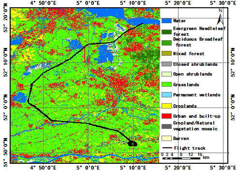
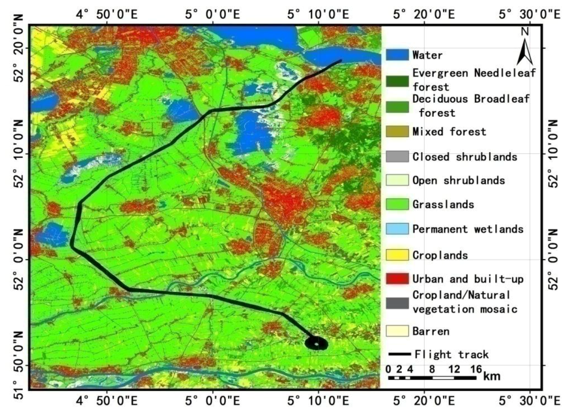
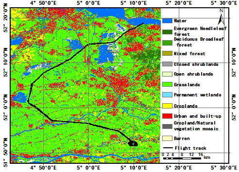
2. Study Area and Data Description

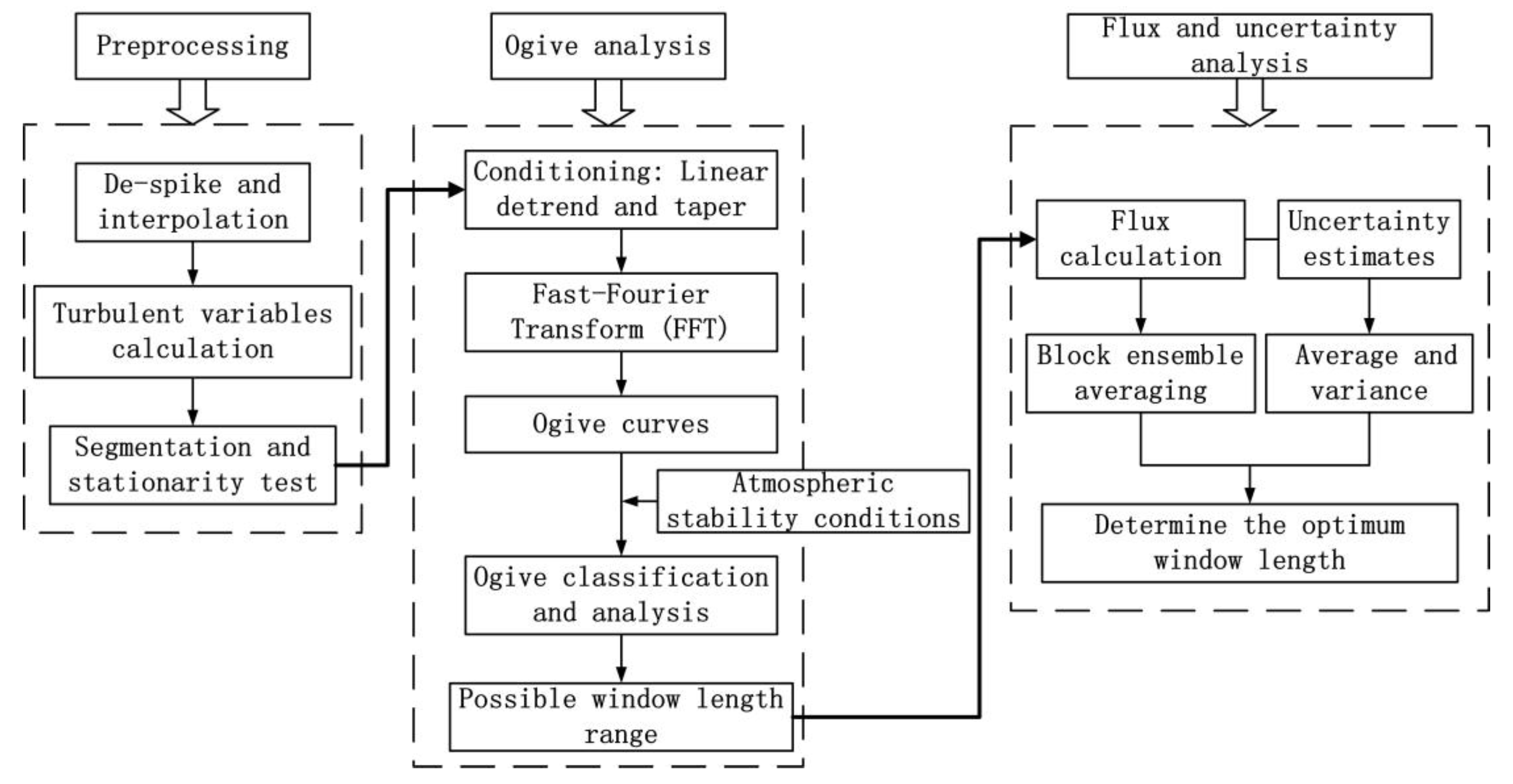
Airborne EC measurements were carried out between March 2008 and February 2009 in the Netherlands using Sky Arrow 650 aircraft by means of flying at a low altitude and low speed [49,50]. Flights were performed along three different trajectories that covered all of the major land cover types of the Netherlands. This environmental research aircraft is equipped with a Mobile Flux Platform (MFP) system, which consists of a Best Atmospheric Turbulence (BAT) probe [51], a thinwire thermocouple, and an LI-COR 7500 infrared gas analyzer (IRGA) for fluxes of heat, water vapor, and carbon dioxide at a frequency of 50 Hz. More detailed descriptions of this particular aircraft and the 2008 campaign in the Netherlands can be found elsewhere [31,42,50,52].

The study area and flight transections employed in this study are displayed in Figure 1 over the land cover classification map. For land cover information, the LGN6 database was used [53]. The spatial resolution of the land cover map is 25 m, and 39 land cover types are distinguished in the land cover map. We regrouped original land cover classes into 12 classes according to the IGBP classification scheme for simplifying. The study area selected by this study (Figure 1) is located in the west of the Netherlands (between 4.69–5.21°E and 51.83–52.28°N). The land cover in this domain is dominated by grasslands, which are studded with some croplands, water surfaces, and construction lands.

Table 1. Summary of the whole flights during the 2008 in the west of the Netherlands (Figure 1). Including measurement date, time (coordinated universal time, UTC), flight height (above ground level, m), and Monin–Obukhov (M–O) stability parameter $\mathsf{\zeta }$.

Date	Time (UTC)	Altitude (m)	M–O Stability ($\mathsf{\zeta }$)
29 February 2008	13:03–13:53	57	−0.04
11 April 2008	11:14–11:47	67	−10.03
11 April 2008	12:29–13:03	65	−10.27
2 May 2008	10:58–11:30	71	−1.08
2 May 2008	11:53–12:25	78	−0.63
23 May 2008	08:32–09:05	68	−2.24
23 May 2008	09:41–10:14	69	−3.82
13 June 2008	10:19–10:50	76	−0.32
13 June 2008	11:07–11:40	71	−0.47
4 July 2008	11:32–12:05	66	0.05
4 July 2008	12:32–13:08	66	0.01
25 July 2008	09:52–10:23	66	−0.34
25 July 2008	10:51–11:20	68	−0.35
15 August 2008	10:25–11:01	66	−0.22
15 August 2008	11:30–12:06	66	−0.36
5 September 2008	09:10–09:39	63	−0.12
17 October 2008	13:27–13:59	73	−0.26
31 October 2008	13:08–13:39	69	−0.43
11 December 2008	13:48–14:24	74	0.02

summarizes the 19 transect flights carried out in the selected area. All of the flights were flown during the daytime. The measurement height was approximately 68 m. From the vertical profile flight carried out during each field measurements, the boundary layer depth was estimated to be around 800–1100 m for all flight periods. We can confirm that all of the flight levels were within the near surface layer (approximately 10% of the depth of the boundary layer), and we neglected the fluctuation of surface layer height existing in different flights [54,55]. Figure 1 shows that the predominant land cover type under the airline is grassland, and no flight paths were directly across lakes. In the current study, we applied the Monin–Obukhov (M–O) stability parameter as the indicator of atmospheric stability [56], denoted as $\mathsf{\zeta }$. It is defined as $\mathsf{\zeta }=\mathrm{z}/{\mathrm{L}}_{*}$, where ${\mathrm{L}}_{*}$ is the Obukhov length (m) [57] and $\mathrm{z}$ is the measurement height (m). The Obukhov length (${\mathrm{L}}_{*}$) is defined as:

$${\mathrm{L}}_{*}=-\frac{{\mathrm{u}}_{*}{}^3}{\mathsf{\kappa } \frac{\mathrm{g}}{\overline{{\mathsf{\theta }}_{\mathrm{v}}}} \overline{{\mathsf{\theta }}_{\mathrm{v}}^{\prime }{\mathrm{w}}^{\prime }}}$$

(1)

where ${\mathrm{u}}_{*}$ is the friction velocity (ms⁻¹), $\mathsf{\kappa }=0.4$ is the von Karman constant, $\mathrm{g}$ is the acceleration of gravity (ms⁻²), ${\mathsf{\theta }}_{\mathrm{v}}$ is the virtual potential temperature (K), $\mathrm{w}$ is the vertical wind component (ms⁻¹), and $\overline{{\mathsf{\theta }}_{\mathrm{v}}^{\prime }{\mathrm{w}}^{\prime }}$ is the buoyancy flux. As listed in Table 1, a wide range of atmospheric stability conditions from near neutral ($\mathsf{\zeta }=0.05$) to very unstable ($\mathsf{\zeta }=-10.03$) were considered in this study. In addition, the terrain in this field is flatter than that in other regions. The relatively uniform land cover and the flat terrain make this region more appropriate for our research objective than other places measured during the 2008 flight campaign in The Netherlands.

3. Methods

The methodological framework of this study is illustrated in Figure 2. The procedure includes three parts. First, the raw data were preprocessed, including de-spike, segmentation, and steady-state test. Then, the Ogive analysis for turbulent heat flux from all available segmentations was used to determine the possible window length range under near neutral to unstable atmospheric stability conditions. Lastly, the possible window lengths from the Ogive analysis were employed to calculate the turbulent heat fluxes and their uncertainty, and based on which we defined the final optimum window length. Detailed methods are described in the following sections.

3.1. Data Preprocessing

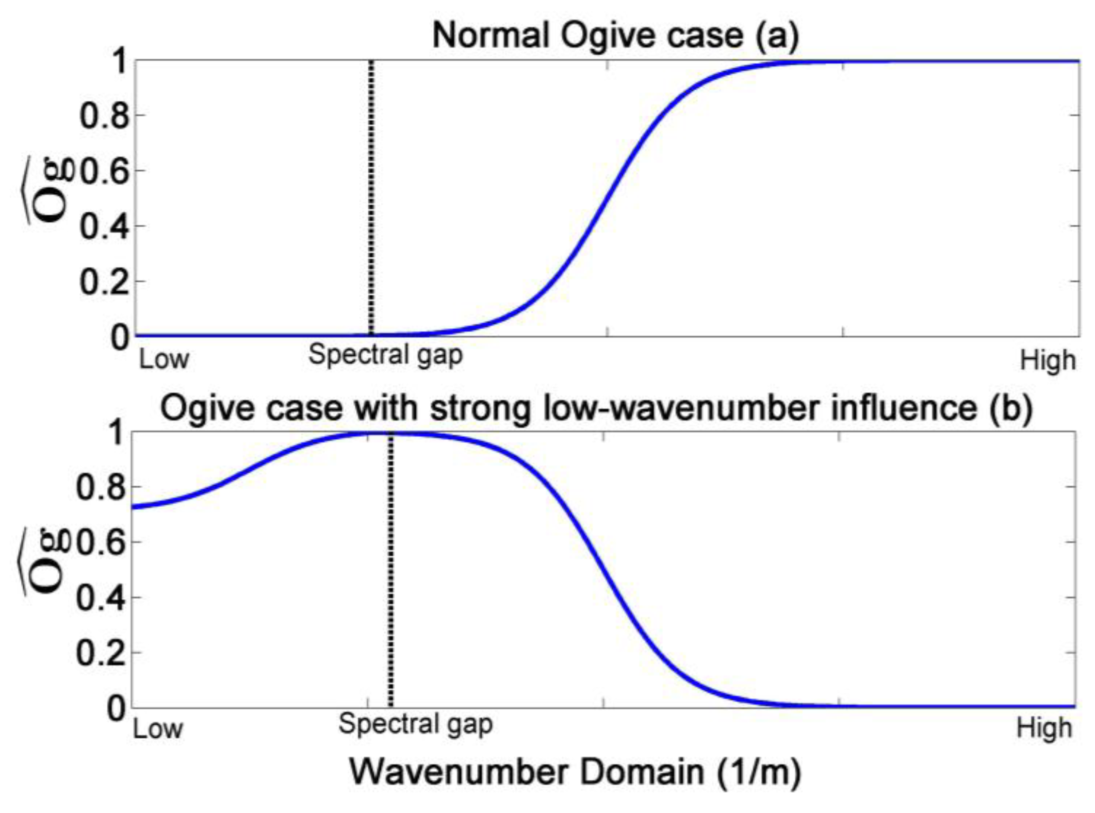
Both the EC method and spectral analysis require raw data with no noise, no missing values, and meeting the stationary condition [12]. In the first stage, the raw data from airborne EC measurements needed to be checked for outliers. We used the same method as Vellinga et al. [42,44] to detect the spikes and fill the gaps using linear interpolation. In the second stage, turbulent variables such as wind components, true airspeed, and (dry) air density were calculated [25,42,44].

In order to fulfill the stationary requirement, continuous observations are typically subdivided into several identical segments [12]. The segments should be both sufficiently long to include the fluxes contained in the large eddies and short enough to avoid departures from the stationary condition [58]. In the present study, we adopted 10 km as the segment length, which is long enough to include the main scales of turbulent transporting in the study area as well as to maintain the quasi-stationary conditions. Shorter segment lengths were not investigated for the purpose of investigating the behavior of the low-frequency turbulence, and longer segment lengths were not investigated due to their high nonstationary conditions. The underlying assumption of a 10 km segment length is that no significant scalar or momentum flux contributions were from eddies larger than 10 km [59].

After subdividing the whole flight data into segments, we obtained 113 segments data. Then, the stationarity test was executed to ensure that the segments are near stationary. The stationarity test is based on a relative nonstationarity factor, ${\mathrm{RN}}_{\mathsf{\xi }\mathrm{w}}$, proposed by Foken and Wichura [9]. This factor compares the statistical parameters determined for the entire segment and for short intervals within this segment, expressed as:

$${\mathrm{RN}}_{\mathsf{\xi }\mathrm{w}}=\left|\frac{\overline{{\mathsf{\xi }}^{\prime }{\mathrm{w}}^{\prime }}-{\overline{{\overline{{\mathsf{\xi }}^{\prime }{\mathrm{w}}^{\prime }}}_{\mathrm{j}}}}^{\mathrm{J}}}{\overline{{\mathsf{\xi }}^{\prime }{\mathrm{w}}^{\prime }}}\right|$$

(2)

where $\overline{{\mathsf{\xi }}^{\prime }{\mathrm{w}}^{\prime }}$ is the covariance between $\mathsf{\xi }$ (horizontal wind component or scalar) and $\mathrm{w}$ (vertical wind, ms⁻¹) for the entire segment, ${\overline{{\mathsf{\xi }}^{\prime }{\mathrm{w}}^{\prime }}}_{\mathrm{j}}$ is the covariance of a given interval j in the segment, and ${\overline{{\overline{{\mathsf{\xi }}^{\prime }{\mathrm{w}}^{\prime }}}_{\mathrm{j}}}}^{\mathrm{J}}$ is the average of all the covariances in J non-overlapping intervals with equal length into which the segment is divided. The segment is stationary if the nonstationarity factor (${\mathrm{RN}}_{\mathsf{\xi }\mathrm{w}}$) is less than a threshold (usually 0.3). In this study, we split the segment into five intervals (J = 5) and used the value ${\mathrm{RN}}_{\mathsf{\xi }\mathrm{w}}\le 1$ as a criterion. A segment with ${\mathrm{RN}}_{\mathsf{\xi }\mathrm{w}}\le 1$ is acceptable for general use, according to Foken et al. [9] and Vellinga et al. [42]. It is a relaxed criterion, enabling us to obtain the most segments to analyze. Moreover, if one segment of data contains more than 10% spikes, the segment will be discarded. After the preprocessing, we were left with 111 segments to be used for the Ogive analysis, described in the next section.

3.2. Ogive Analysis

All turbulent variables are linearly detrended (LDT) and tapered using the Hamming window within each segment to reduce the spectral leakage (sharp edge) according to Kaimal et al. [58]. The turbulence spectral leakage was introduced by the implicit assumption in Fourier analysis that the segment under consideration is infinitely periodic [60]. Then, we employed the fast Fourier transform (FFT) to decompose the sensible and latent heat covariance into frequency-dependent contributions, by which the discrete (co)spectral intensities were obtained. The main interest in calculating the (co)spectrum is that the integral of the (co)spectrum over the whole frequency range is equal to the (co)variance of the signal; thus, the (co)spectrum could be taken as a distribution of (co)variances in different frequency bands [60].

The Ogive analysis is a common method to determine the optimal averaging time or length to capture most of the flux-carrying eddies [12,17,23]. It is defined as the cumulative integral of the cospectrum of the turbulent flux from the lowest frequency to the highest frequency, expressed as:

$${\mathrm{Og}}_{\mathsf{\xi }\mathrm{w}}\left(f_0\right)={{\displaystyle \int }}_{\infty }^{f_0}{\mathrm{Co}}_{\mathsf{\xi }\mathrm{w}}\left(f\right)\mathrm{d}f$$

(3)

where ${\mathrm{Co}}_{\mathsf{\xi }\mathrm{w}}$ is the cospectrum of a turbulent flux, $\mathrm{w}$ is the vertical wind component (ms⁻¹), $\mathsf{\xi }$ is the horizontal wind component or scalar, $f$ is the frequency (Hz), and $f_0$ is the Nyquist frequency (Hz). If the Ogive curve approaches an asymptote over the low-frequency domain, it may provide information about the minimum window length required to capture all flux-carrying turbulence scales, which is very import for airborne EC measurements to resolve the turbulence signal from surface heterogeneity. The Ogive analysis allows us to certify whether the fluxes converge to an asymptote within the window length [61]. If the Ogive curve converges to a predefined asymptote (0.1 in this study) at a frequency over the low-frequency domain, then a cospectral gap is existent [17]. In this study, we used wavenumber (k, 1/m) instead of frequency because the reciprocal of the wavenumber corresponds to the wavelength of eddies. The wavenumber is defined as $\mathrm{k}=f/\overline{\mathrm{u}}$, where $\overline{\mathrm{u}}$ is the average speed (ms⁻¹) of flight within one segment. The low-wavenumber components of turbulence are connected with the surface heterogeneity and may lead to the Ogive curve not converging over the low-wavenumber range [12]. Moreover, the spectral gap may disappear during the significant overlap of high-wavenumber and low-wavenumber components of turbulence. In such a situation, it is impossible to separate the flux contributions by adjusting the window length [17].

In this study, we defined the normalized Ogive for the purpose of convenience in comparison, denoted as ${\widehat{\mathrm{Og}}}_{\mathsf{\xi }\mathrm{w}}$. It is expressed as the Ogive values normalized by the maximum absolute value of the Ogive function with its sign:

$${\widehat{\mathrm{Og}}}_{\mathsf{\xi }\mathrm{w}}\left(\mathrm{k}\right)=\frac{{\mathrm{Og}}_{\mathsf{\xi }\mathrm{w}}\left(\mathrm{k}\right)}{\mathrm{sgn}\left\{\max \left({\mathrm{Og}}_{\mathsf{\xi }\mathrm{w}}\left(\mathrm{k}\right)\right)+\min \left({\mathrm{Og}}_{\mathsf{\xi }\mathrm{w}}\left(\mathrm{k}\right)\right)\right\}\max \left(\left|{\mathrm{Og}}_{\mathsf{\xi }\mathrm{w}}\left(\mathrm{k}\right)\right|\right)}$$

(4)

where $\mathrm{sgn}\{ \}$ is the signum function that returns +1 if its argument is positive, −1 if its argument is negative, and 0 if its argument is zero. In Equation (4), it returns the sign of the maximum absolute value of the Ogive function. So, at the frequency corresponding to the peak (the maximum absolute value) of the Ogive curve, the value of the normalized Ogive is 1. Figure 3 provides a diagram clarifying Equation (4). In the normal Ogive case (Figure 3a), turbulent flux and low-wavenumber turbulence are clearly separated by a spectral gap. An extreme situation may occur when the absolute maximum value of Ogive curve presents in the low-wavenumber range and has an opposite sign to the Ogive values in the high-wavenumber range. In this case, the Ogive curves of our definition would exhibit reversed shape compared with normal Ogive curves (Figure 3b), rendering it easy to identify the opposite sign and relatively strong influence of low-wavenumber components of turbulence. In reality, the Ogive curve of real turbulence data is very complicated, mainly due to the low-wavenumber motion of turbulence. We shall give a detailed analysis the Ogive cases of our data segments in the Results section.

3.3. Uncertainty Estimation

The total uncertainty of EC measurements can be attributed to random and systematic errors [62]. Details of the flux sampling errors of aircraft measurement can be found in Mahrt [63]. Experimental studies [64] and theoretical considerations [19] have shown that the main uncertainty of airborne flux measurements is due to the presence of significant flux contribution at wavelengths that are not covered by the window length [26]. However, care must be taken to prevent the window length from exceeding the length over which the flow is nonstationary [36,65]. In this study, we assumed that the preprocessing steps have reduced sufficiently the systematic measurement errors from instrumentation. We assumed that the major source of uncertainty in the airborne flux measurements is from an inappropriate window length through under-sampling or over-sampling at some turbulence scales. According to Mauder et al. [62], the uncertainty in flux estimates is associated with the stochastic error of turbulence. The stochastic error depends on the number of independent observations, which is determined by the turbulence integral scale [19]. The turbulence integral scale is a measure of the length for which the variables are correlated (i.e., not an independent observation) [62]. Consequently, the uncertainty is associated with both the sampling length and the stationary condition of the turbulence. This means that extending the window length to ensure adequate sampling could decrease the uncertainty. However, an overly long window length may result in a departure from statistical stationarity and thus increase the uncertainty.

Several methods have been introduced and compared to estimate the flux uncertainty [66]. These methods rely on estimating the turbulence integral scale [67]. However, the integral scale is not always estimated reliably [19]. We adopted the algorithm of Finkelstein and Sims [67] to estimate the flux uncertainty as the statistical variance of the covariance, which is a statistically profound and mathematically rigorous approach (Appendix A). Subsequently, we accounted for the effects of the propagation of uncertainty, following the method from Billesbach [66], as outlined in Appendix A. Combined with Equation (A5), we could diagnose the absolute uncertainty for sensible heat flux, denoted as ${\mathsf{\sigma }}_{{\mathrm{F}}_{\mathrm{H}}}$, and for latent heat flux, denoted as ${\mathsf{\sigma }}_{{\mathrm{F}}_{\mathrm{LE}}}$, using Equations (A9) and (A10). It is instructive to express the uncertainties relative to the magnitude of the flux (denoted as ${\mathrm{F}}_{\mathrm{H}}$ and ${\mathrm{F}}_{\mathrm{LE}}$ for sensible and latent heat flux, respectively). For the sensible heat flux, the relative flux uncertainty (${\mathrm{R}}_{\mathrm{H}}$) can be expressed as:

$${\mathrm{R}}_{\mathrm{H}}= \frac{{\mathsf{\sigma }}_{{\mathrm{F}}_{\mathrm{H}}}}{\left|{\mathrm{F}}_{\mathrm{H}}\right|}$$

(5)

and for the latent heat flux, the relative flux uncertainty (${\mathrm{R}}_{\mathrm{LE}}$) can be expressed as:

$${\mathrm{R}}_{\mathrm{LE}}= \frac{{\mathsf{\sigma }}_{{\mathrm{F}}_{\mathrm{LE}}}}{\left|{\mathrm{F}}_{\mathrm{LE}}\right|}$$

(6)

3.4. Block Ensemble Averaging

We assumed that one specified window length divided the 10 km segment into N consecutive blocks. Block ensemble averaging means that the fluxes of each block are averaged to form an ensemble flux of this segment. This block ensemble averaged flux becomes a function of window length because the size and the number of the block is decided by the window length. In the current study, the block ensemble averaged flux could be used to describe the evolution of flux with respect to the window length. We used the angle brackets 〈 〉 to denote the block ensemble average. Let ${\mathrm{F}}_{\mathrm{n}}$ denote the flux of the $\mathrm{nth}$ block in a series of N consecutive block flux values, each with window length $\mathrm{L}$ [10,63,68,69]. The block ensemble averaged flux of all of the $\mathrm{N}$ blocks within a segment can be expressed as:

$$\overline{\langle {\mathrm{F}}_{\mathrm{L}}\rangle }= \frac{1}{\mathrm{N}}{\displaystyle \sum }_{\mathrm{n}=1}^{\mathrm{N}}{\mathrm{F}}_{\mathrm{n}}$$

(7)

Then, we obtained a series of block ensemble averaged fluxes based on different window lengths ($\mathrm{L}$) for a segment. For the convenience of comparison, we adopted a processing manner similar to normalization to normalize these block ensemble averaged fluxes as:

$${\mathrm{E}}_{\mathrm{L}}= \frac{\left|\overline{\langle {\mathrm{F}}_{\mathrm{L}}\rangle }\right|}{\max (\left|\overline{\langle {\mathrm{F}}_{\mathrm{L}}\rangle }\right|)}$$

(8)

where ${\mathrm{E}}_{\mathrm{L}}$ is the block ensemble averaged non-dimensional flux. Relative flux uncertainties were estimated along with flux calculation. We also calculated the average and standard deviation (SD) of relative flux uncertainties under different window lengths to study the evolution of uncertainties relative to window length. For the block ensemble averaged non-dimensional fluxes, a four-point running mean filter was used to clearly demonstrate the trends of fluxes as a function of window length.

4. Results

4.1. Ogive Analysis

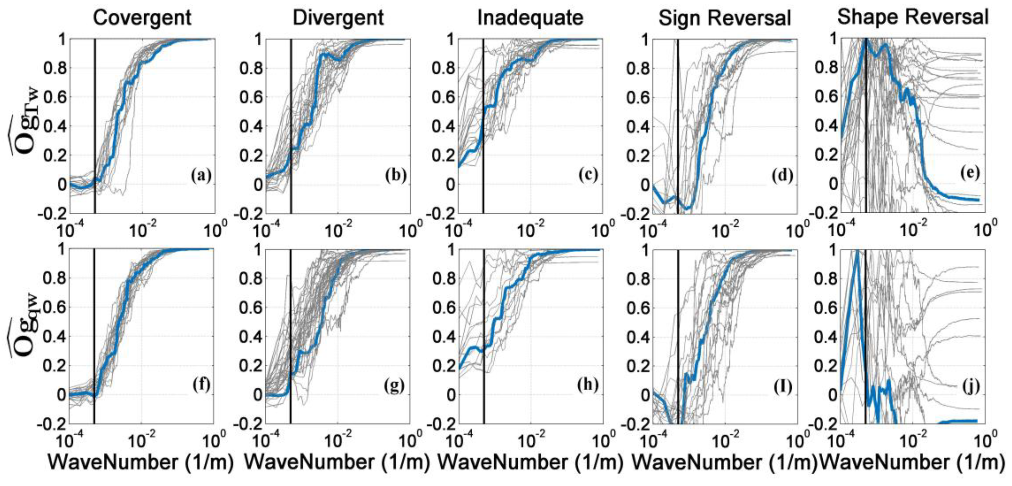
4.1.1. Classification of Ogive Curves

In the following, we employed a window length of 2 km as a reference to investigate the convergence of the Ogive curves. The Ogive function integrates the cospectrum from the low-wavenumber to the high-wavenumber to clearly reveal the low-wavenumber behavior of the turbulent flux. Then, similar to Foken et al. [12], we split the behavior of the Ogive curves into one of five cases: (1) convergent; (2) divergent; (3) inadequate; (4) sign reversal; and (5) shape reversal. Different from Foken et al. [12], we excluded the “extreme” case because this case occurred infrequently in our segments (it only accounted for 2.7% in Ogives of sensible heat flux and no extreme cases were found in Ogives of latent heat flux). Moreover, we included more “inadequate”, “sign reversal”, and “shape reversal” cases in order to achieve a detailed description of the low-wavenumber behavior of turbulence, which was not considered by Foken et al. [12].

Table 2. Definition of five different cases for the behavior of Ogive curves of turbulent fluxes.

Case	Explanation	Criterion
(1) Convergent	Convergent within the 2 km interval. Ideal case.	${\widehat{\mathrm{Og}}}_{\mathsf{\xi }\mathrm{w}}\left({\mathrm{k}}^{-1}=10 \mathrm{km}\right)<0.1$ and ${\widehat{\mathrm{Og}}}_{\mathsf{\xi }\mathrm{w}}\left({\mathrm{k}}^{-1}=2 \mathrm{km}\right)<0.1$
(2) Divergent	Ogive curve is not convergent within 2 km interval, but is convergent in the wavelength larger than 2 km. Window length should be longer.	${\widehat{\mathrm{Og}}}_{\mathsf{\xi }\mathrm{w}}\left({\mathrm{k}}^{-1}=10 \mathrm{km}\right)<0.1$ and ${\widehat{\mathrm{Og}}}_{\mathsf{\xi }\mathrm{w}}\left({\mathrm{k}}^{-1}=2 \mathrm{km}\right)>0.1$
(3) Inadequate	Ogive curve is not convergent even for 10 km interval. Unclear cospectral gap.	${\widehat{\mathrm{Og}}}_{\mathsf{\xi }\mathrm{w}}\left({\mathrm{k}}^{-1}=10 \mathrm{km}\right)>0.1$ and ${\widehat{\mathrm{Og}}}_{\mathsf{\xi }\mathrm{w}}\left({\mathrm{k}}^{-1}=2 \mathrm{km}\right)>0.1$ and $\min \left({\widehat{\mathrm{Og}}}_{\mathsf{\xi }\mathrm{w}}\left(\mathrm{k}\right)\right)>0.1$
(4) Sign Reversal	Ogive curve undergoes a relatively large sign reversal in low-wavenumber domain while maintaining the normal Ogive shape.	${\widehat{\mathrm{Og}}}_{\mathsf{\xi }\mathrm{w}}\left(\mathrm{k}\right)\le -0.1$ and ${\widehat{\mathrm{Og}}}_{\mathsf{\xi }\mathrm{w}}\left({\mathrm{k}}^{-1}<10 \mathrm{m}\right)\ge 0.9$
(5) Shape Reversal	Ogive curve undergoes a very large sign reversal and displays reversed shape compared with other cases.	${\widehat{\mathrm{Og}}}_{\mathsf{\xi }\mathrm{w}}\left(\mathrm{k}\right)\le -0.1$ and ${\widehat{\mathrm{Og}}}_{\mathsf{\xi }\mathrm{w}}\left({\mathrm{k}}^{-1}<10 \mathrm{m}\right)<0.9$

provides the detailed definitions of the five cases for the behavior of Ogive curves of turbulent fluxes. We began with the last two cases (Case 4 and Case 5 in Table 2), shown by the gray curves in the right two column panels in Figure 4. The sign reversal Ogive (Case 4) and the shape reversal Ogive (Case 5) share a commonality, that there exists a wavenumber at which the Ogive value is more than one-tenth the magnitude of the absolute maximum value of the Ogive, but with the opposite sign. We used the normalized Ogive value of −0.1 as the threshold, because we considered the sign changes of Ogive values exceeding 10% to be intolerable. This is based on the theory that significant contributions of turbulent fluxes from eddies always share the same sign, regardless of the size [22,70]. In contrast, the “sign reversal” case (Figure 4d,I) means that the Ogive curve undergoes a relatively large sign reversal in the low-wavenumber domain, while the convergent value of the Ogive curve in the high-wavenumber domain is larger than 0.9. The “shape reversal” case (Figure 4e,j) means that the Ogive curve exhibits the reversed shape compared with other cases (it occurs when the convergent value of the Ogive curve in the high-wavenumber domain is less than 0.9). The other cases used the normalized Ogive value of 0.1 as the criterion value based on the same consideration as Foken et al. [12], that is, only accepting the variability of the convergent value of the Ogive curve within 10% in the low-wavenumber domain.

Case 1, as shown by the gray curves in Figure 4a,f, is the ideal convergent case. The Ogive function converged to a predefined range (0.1 to ~−0.1) in the low-wavenumber end within the reference window length of 2 km. For an Ogive of convergence, the 2 km window length is a reliable estimate of the turbulent flux, as we can assume that the whole turbulent cospectrum is “captured” within this window length and there are only negligible flux contributions from the longer wavelength domain [12].

Case 2, as shown by the gray curves in Figure 4b,g, is the divergent case. The Ogive function value from the 10 km window length converged to the predefined range (−0.1 to ~0.1), meanwhile the Ogive value from the 2 km window length is greater than the threshold value (0.1). This indicates that the flux continues to increase significantly in magnitude beyond the 2 km window length. A longer window length is needed to capture more flux contributions.

Case 3, as shown by the gray curves in Figure 4c,h, is the inadequate case. The Ogive function does not reach the threshold value of 0.1, even with the 10 km segment length. This means that the linear detrend has only excluded the mesoscale transports of turbulence with spatial scales of 10 km. In this case, the flux is underestimated, even using the 10 km window length. This is because the energy is also transported by large eddies of a size larger than 10 km [12]. In the current study, no clear spectral gap could be found in this case. So, it is hard to determine a good choice of window length for “inadequate case”.

The sign reversed cases and the shape reversed cases are all caused by the significant negative flux influence by low-wavenumber components of turbulence, but few studies have dealt with this issue. Possible reasons for this may be that the direction of mesoscale turbulence is opposite that of local turbulent transporting [68]. In the following, we combined the sign reversed and shape reversed cases as a unique reversed Ogive case and analyzed the case-wise fractions of Ogive cases under different stability conditions. Because fluxes measured under stable conditions (here, $\mathsf{\zeta }>0.2$) are always inaccurate, we discarded the segments under stable conditions, which accounted for less than 2.6% of all segments. Then, the segments were classified into three stability conditions: neutral conditions ($\left|\mathsf{\zeta }\right|\le 0.2$), moderately unstable conditions ($-1\le \mathsf{\zeta }<-0.2$), and very unstable conditions ($\mathsf{\zeta }< -1$).

Table 3. Classification fractions of the Ogives for sensible heat flux (corresponding to upper panels in Figure 2). The numbers are the fraction of Ogives in a given category (column) under the given classification (row).

Ogive Case (${\widehat{\mathbf{O}\mathbf{g}}}_{\mathbf{T}\mathsf{\omega }}$)	Neutral (%)	Moderately Unstable (%)	Very Unstable (%)	All Stabilities (%)
Case 1: Convergent	11.6	15.2	23.8	15.5
Case 2: Divergent	7	34.8	38.1	24.5
Case 3: Inadequate	16.3	21.7	23.8	20
Case 4 and Case 5: Reversed	62.8	26.1	9.5	37.3

presents the classification fractions of the Ogives for sensible heat flux under each stability condition. Overall, the reference window length of 2 km did not perform well for the reason that only 15.5% of Ogive curves were convergent. Plenty of Ogive curves presented the reversed case (37.3%), the divergent case (24.5%), and the inadequate case (20%), respectively. Under neutral atmospheric stability conditions, the reversed case accounted for 62.8%, which is the highest portion compared with other cases. Under moderately unstable atmospheric stability conditions, the divergent cases accounted for the largest portion (34.8%), followed by the inadequate cases (21.7%) and the reversed cases (26.1%). The proportion of convergent cases under moderately unstable conditions was 15.2%, which is larger than the proportion of convergent cases under neutral conditions (11.6%). Under very unstable atmospheric stability conditions, the proportion of divergent cases was the largest (38.1%), followed by the inadequate cases (23.8%) and the convergent cases (23.8%). Under this condition, the proportion of reversed cases was 9.5%, which is the lowest compared with other conditions. Following the evolution of atmospheric stability from neutral to very unstable conditions, the proportion of convergent, divergent, and inadequate cases gradually increased. On the contrary, the proportion of reversal cases was significantly reduced with the development of instability. Under moderately unstable and very unstable conditions, the high proportion of divergent cases indicates that a window length longer than 2 km is needed.

Table 4. Classification fractions of the Ogives for latent heat flux (corresponding to bottom panels in Figure 2). The numbers are the fraction of Ogives in a given category (column) under the given classification (row).

Ogive Case (${\widehat{\mathbf{O}\mathbf{g}}}_{\mathbf{q}\mathsf{\omega }}$)	Neutral (%)	Moderately Unstable (%)	Very Unstable (%)	All Stabilities (%)
Case 1: Convergent	27.9	15.2	18.2	20.7
Case 2: Divergent	20.9	43.5	59.1	37.9
Case 3: Inadequate	11.7	19.6	4.5	13.5
Case 4 and Case 5: Reversed	39.5	21.7	18.2	27.9

depicts the classification fractions of the Ogives for latent heat flux under each stability condition. Analogous to the sensible heat flux, the window length of 2 km for latent heat flux calculation was inappropriate, as only 20.7% of Ogive curves were found to be convergent. Meanwhile, the portion of divergent and reversed cases were relatively significant, accounting for 37.9% and 27.9%, respectively. Under neutral atmospheric stability conditions, the proportion of reversed cases was the largest, accounting for 39.5%. The proportion of convergent cases was 27.9%, which was more than the proportions of divergent cases (20.9%) and inadequate cases (11.7%). Under moderately unstable atmospheric stability conditions, the proportion of divergent cases was the largest (43.5%), followed by the reversed cases (21.7%). The proportion of inadequate cases under moderately unstable conditions was 19.6%, and the proportion of convergent cases was only 15.2%. Under very unstable atmospheric stability conditions, the proportion of divergent cases reached up to 59.5%, followed by the convergent cases (18.2%) and the reversed cases (18.2%). The proportion of inadequate cases was only 4.5%. From the evolution of atmospheric stability, with the development of instability, the increasing proportion of divergent cases indicates that a window length longer than 2 km is needed under moderate and very unstable conditions. Meanwhile, the proportion of reversed cases significantly decreased, which is the same as its evolution for sensible heat flux.

By comparing Table 3 and Table 4, some difference in the behavior of Ogive cases between sensible and latent heat fluxes can be seen. The Ogives of latent heat fluxes present higher proportions of convergent and divergent cases and lower proportions of inadequate and reversed cases compared to Ogives of sensible heat fluxes under all atmospheric stability conditions. This difference is related to the physical mechanism of sensible and latent heat fluxes. According to Kustas et al. [71], the transport of heat is more tightly coupled with local surface discontinuities, whereas the moisture flux has additional mechanisms influencing its transport. From the results of large eddy simulation (LES), the water vapor flux blends or mixes more efficiently than sensible heat flux because water vapor is a passive scalar, as opposed to temperature, which is an active scalar affecting vertical velocity through the buoyancy term [70]. Thus, the vertical transport sensible heat flux generated over the local land surface does not mix horizontally as efficiently as water vapor [71]. As mentioned by Mahrt et al. [72], the mixing of water vapor in the daytime convective mixed layer reduces the relative influence of surface heterogeneity and increases the horizontal mixing scale of turbulence. We also found some similarities of Ogive behavior between the sensible and latent heat fluxes in our study. On the one hand, the proportion of divergent cases was dominant under moderate and very unstable conditions for both the Ogives of sensible and latent heat fluxes. This illustrated that the size of eddies, which is associated with the transport of local turbulent fluxes, increased notably from neutral to very unstable atmospheric stability conditions. This is consistent with the consensus on turbulence spectra [73,74], that under unstable atmospheric stability conditions, the cospectra gap shifts toward the low-wavenumber components of turbulence [75]. Consequently, a window length longer than 2 km is needed to include the significant flux contribution from large eddies. On the other hand, the proportion of reversed cases decreased significantly with the development of instability. This indicates that, as the mixing of local turbulence becomes more and more efficient, the negative influence of the mesoscale turbulence associated with surface heterogeneity is reduced.

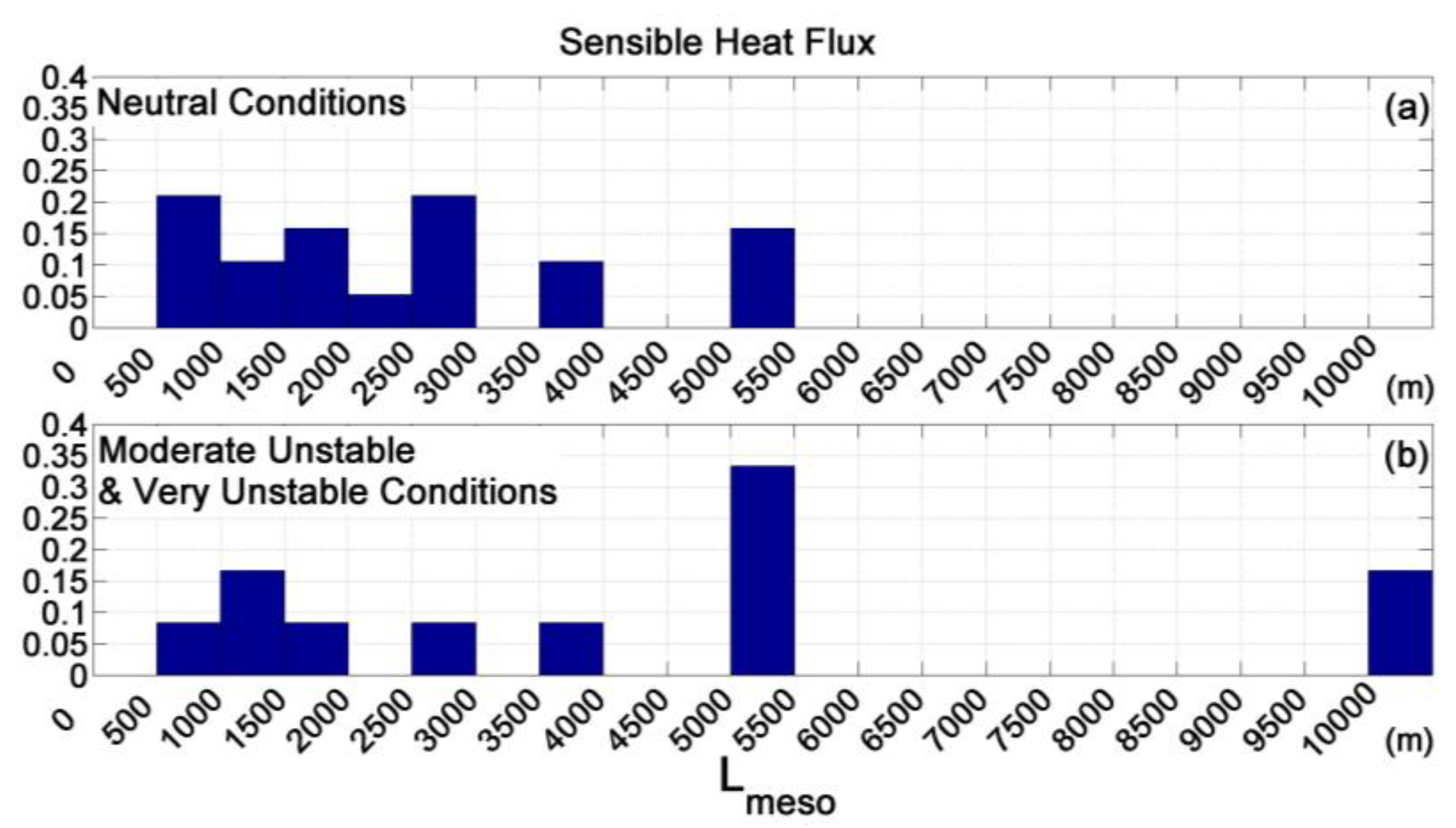
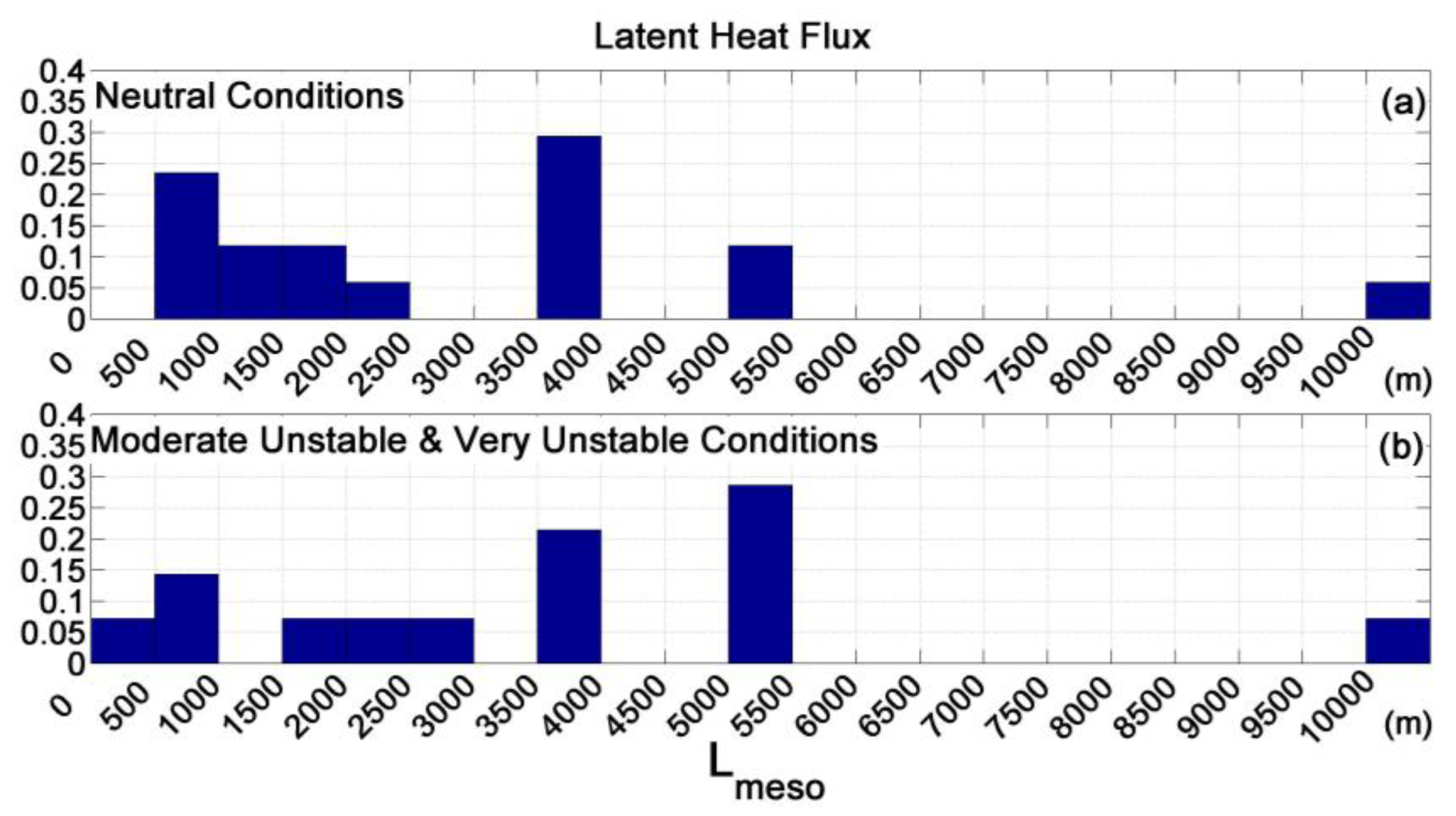
4.1.2. Determination of Possible Window Length

As mentioned above, we can confirm that the window length should be larger than 2 km under moderately unstable and very unstable conditions. However, it is hard to determine the suitable window length under near neutral conditions due to the complexity of the reversed case, which was the most common case in such conditions. Even under other conditions, the reversed case still occupied a significant portion and thus should not be ignored. Inappropriate window length can potentially cause an underestimation of fluxes when the reversed case occurs.

For the purpose of determining the typical size of mesoscale eddies that result in the reversed case, we defined different regulations to obtain the wavelength in the low wavenumber at which the sign reversal occurs; this wavelength is referred to as ${\mathrm{L}}_{\mathrm{meso}}$. For the sign reversed cases, ${\mathrm{L}}_{\mathrm{meso}}$ is the reciprocal of the wavenumber at the lowest point of the Ogive curve (${\mathrm{L}}_{\mathrm{meso}}=\min ({\widehat{\mathrm{Og}}}_{\mathsf{\xi }\mathrm{w}}\left(\mathrm{k}\right))$. For the shape reversed cases, the reciprocal of the wavenumber at the peak of the Ogive curve is the ${\mathrm{L}}_{\mathrm{meso}}$ (${\mathrm{L}}_{\mathrm{meso}}=\max ({\widehat{\mathrm{Og}}}_{\mathsf{\xi }\mathrm{w}}\left(\mathrm{k}\right))$.

Figure 5 shows the frequency histograms of ${\mathrm{L}}_{\mathrm{meso}}$, calculated using the wavelength interval of 500 m for the reversed case of Ogives for sensible heat flux. We noticed that under neutral conditions (Figure 5a) more than 74% of reversed cases are induced by small mesoscale eddies whose typical size (${\mathrm{L}}_{\mathrm{meso}}$) ranges from 500 m to 3000 m. Meanwhile, under moderately unstable and very unstable conditions (Figure 5b), nearly 55% of reversed cases are induced by large mesoscale eddies, whose typical size (${\mathrm{L}}_{\mathrm{meso}}$) ranges from 2000 m to 5500 m. For the reversed case of Ogives for latent heat flux, the results of the frequency histograms of ${\mathrm{L}}_{\mathrm{meso}}$ are shown in Figure 6. Under neutral conditions (Figure 6a), similar to sensible heat flux, most of the reversed cases (53%) are induced by small mesoscale eddies, whose typical size (${\mathrm{L}}_{\mathrm{meso}}$) ranges from 500 m to 3000 m. Under moderately unstable and very unstable conditions (Figure 6b), more than 64% of reversed cases are caused by large mesoscale eddies, whose typical size (${\mathrm{L}}_{\mathrm{meso}}$) ranges from 2000 m to 5500 m. These eddy wavelengths can be considered as the typical size of mesoscale eddies induced by surface heterogeneity. Thus, in the present study, it can be seen that the typical size of mesoscale eddies is ranging from 500 m to 3000 m under near neutral conditions and ranging from 2000 m to 5500 m under moderately and very unstable conditions.

Comparing Figure 5 and Figure 6, we found that the distribution of ${\mathrm{L}}_{\mathrm{meso}}$ of the reversed case for sensible and latent heat fluxes present similar patterns. Under neutral conditions, the size of mesoscale eddies that induced the reversed case is small. Kaimal et al. [73] pointed out that the wavelength of eddies shifted towards shorter from neutral to stable stratification due to the increasing buoyant destruction of turbulence relative to the production of wind shear. In such a situation, large eddies cannot exist [76]. Correspondingly, under moderately and very unstable conditions, large eddies will appear. By re-inspecting the reversed cases of sensible and latent heat fluxes, we found that almost all of the shape reversed cases occurred under near neutral conditions, while most sign reversed cases occurred under moderately and very unstable conditions. The potential explanation for this is that, under neutral conditions, the mixing of local turbulence is insufficient and any small scales of surface heterogeneous could drastically influence the local fluxes and then result in the Ogive curve displaying shape reversal [77]. Under moderately and very unstable conditions, the mixing of turbulence becomes more efficient, and only surface heterogeneity at a large scale or flying through a transition boundary could lead to a relatively large sign reversal in the low-wavenumber domain of the turbulence. Additionally, no reversed case was induced by ${\mathrm{L}}_{\mathrm{meso}}$ between 5500 m and 10,000 m, and a small fraction appeared at the wavelength of 10,000 m (16.6% for Figure 5b, and 5.9% and 7.1% for Figure 6a and 6b, respectively). This revealed that the 10 km segment we selected is long enough to include the main mesoscale turbulence in our study region to conduct the analysis. We thus conclude, based on the analysis of the reversed case, that a short window length is demanded under neutral conditions (smaller than 3000 m) and a long window length, though smaller than 5500 m, is needed under moderately and very unstable conditions.

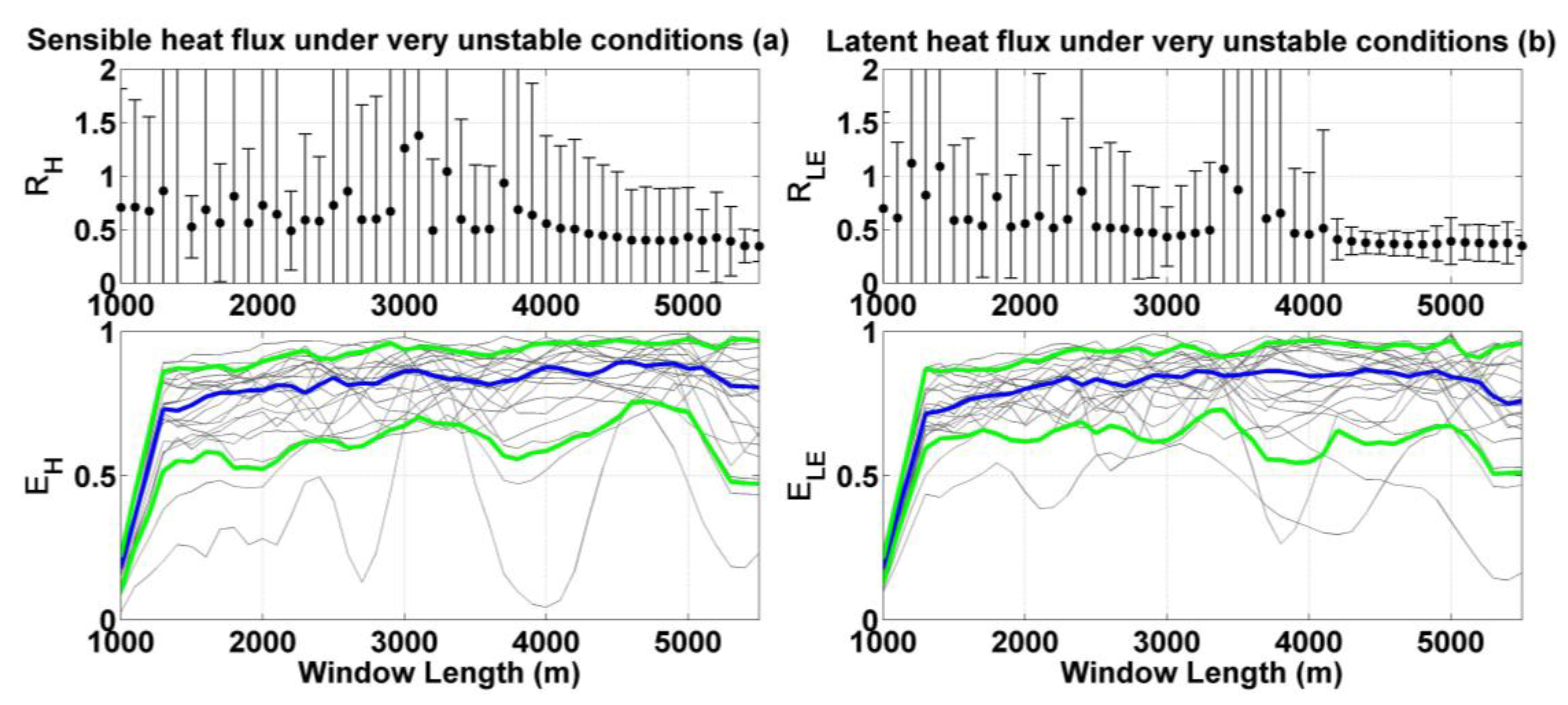
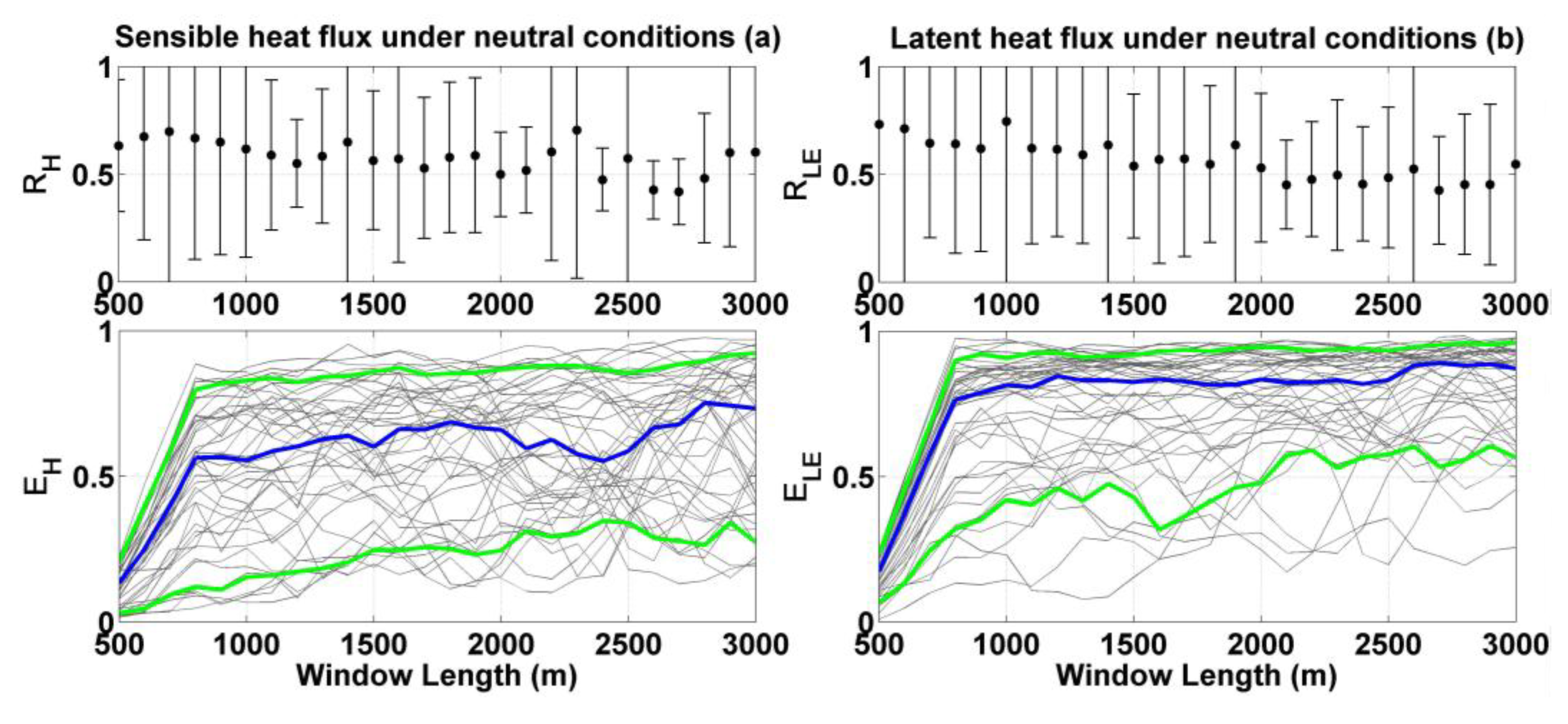
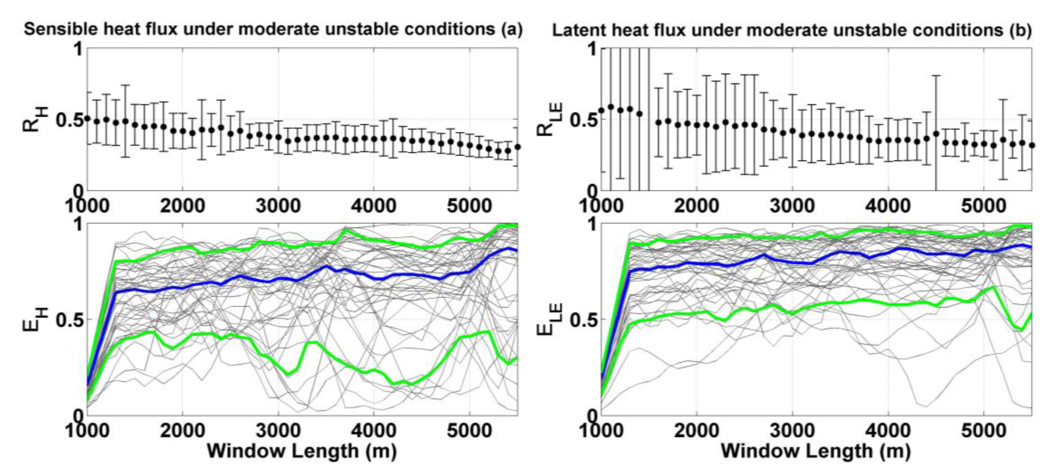
4.2. Uncertainty Associated with the Window Length

According to the results of the Ogive analysis above, we selected several window lengths to calculate the sensible and latent heat fluxes and their relative uncertainties for each segment, to analyze the reliability of flux estimates. Under near neutral conditions, the window lengths ranging from 500 m to 3000 m with 100 m intervals were selected. Under moderately and very unstable conditions, the window lengths ranging from 1000 m to 5500 m with 100 m intervals were employed.

Figure 7 presents the evolution of relative flux uncertainties (${\mathrm{R}}_{\mathrm{H}},{ \mathrm{R}}_{\mathrm{LE}}$) (Equations (5) and (6)) and block ensemble averaged non-dimensional heat fluxes (${\mathrm{E}}_{\mathrm{H}},{ \mathrm{E}}_{\mathrm{LE}}$) (Equation (8)) as a function of window length under near neutral conditions. We used the mean and standard deviation (SD) of relative flux uncertainties under different window lengths to express the evolution of flux uncertainties. From the top panels of Figure 7, the relative uncertainties are reduced upon increasing the window length. Large relative uncertainties occurred between the window lengths of 500 m and 2000 m (mean relative uncertainty bigger than 0.5) because the window lengths were too short to obtain an adequate sample of eddies. Between the window lengths of 2000 m and 2500 m, the relative uncertainties tended to be stable (mean relative uncertainty smaller than 0.5 and its SD smaller than 1) although some fluctuations appeared, probably due to the fact that the relaxed stationarity test we set (with the criterion of ${\mathrm{RN}}_{\mathsf{\xi }\mathrm{w}} \le 1$) may involve some nonstationary turbulence (Section 3.1). After the window length of 2500 m, the uncertainties exhibited large scattering again (mean relative uncertainty bigger than 0.5 and its SD show clearly fluctuations). The large scattering of relative uncertainties after the window length of 2500 m indicated that the increasing window length captured significant nonstationary or heterogeneity turbulence [9,63]. It can be seen in the bottom panels of Figure 7 that the turbulent heat fluxes rapidly increase with the window length increasing from around 500 m to 800 m, then remain stable until the window length reaches about 2500 m. Further increasing in the window length caused significant variability in the turbulent heat flux values due to including the effect of mesoscale turbulence. Finally, combining the heat fluxes and their relative uncertainties for the evolution of the window length, we concluded that the window lengths ranging from 2000 m to 2500 m are optimum for the calculation of local heat fluxes under neutral conditions.

Figure 8 depicts the evolution of relative flux uncertainties (${\mathrm{R}}_{\mathrm{H}},{ \mathrm{R}}_{\mathrm{LE}}$) and block ensemble averaged non-dimensional heat fluxes (${\mathrm{E}}_{\mathrm{H}},{ \mathrm{E}}_{\mathrm{LE}}$) as a function of window length under moderately unstable conditions. In the upper panels of Figure 8, the averaged relative uncertainties were found to be reduced along with the increasing window length. The latent heat flux shows larger uncertainty and scattering than that observed in sensible heat flux. This illustrates that the calculation of latent heat flux demands a longer window length than sensible heat flux to ensure the accuracy of flux estimates. The large scattered relative uncertainties (SD > 0.5) for sensible and latent heat fluxes may be induced by some large eddies that contributed to flux but were not sampled sufficiently. After the window lengths greater than 3900 m, for both sensible and latent heat fluxes, the mean relative uncertainties and their SD start to be less than 0.5 and tend to be stable. Some low-quality observations may have caused a sudden increase among the SD values of relative uncertainty (occurring at the window lengths of 4500 m and 5200 m for latent heat flux), but have little effect on the overall trend, so we ignored these disturbances. From the bottom panels of Figure 8, the values of the flux begin to stabilize at the window length around 1300 m and then remain stable until the window length reaches about 5000 m. The large variation of fluxes after the window length of around 5000 m is probably the result of including mesoscale turbulence. As a consequence, combining the heat fluxes and their relative uncertainties for the evolution of the window length, we concluded that the window lengths ranging from 3900 m to 5000 m are optimum for the calculation of local heat fluxes under moderately unstable conditions.

Figure 9 shows the evolution of relative flux uncertainties (${\mathrm{R}}_{\mathrm{H}},{ \mathrm{R}}_{\mathrm{LE}}$) and block ensemble averaged non-dimensional heat fluxes (${\mathrm{E}}_{\mathrm{H}},{ \mathrm{E}}_{\mathrm{LE}}$) as a function of window length under very unstable conditions. From the top panels in Figure 9, we find that only large window length can obtain a reliable turbulent flux estimates. Significant fluctuation and scattering of relative uncertainties (SD > 1) were observed at window lengths smaller than 4500 m for sensible heat flux and smaller than 4100 m for latent heat flux. The LES results demonstrated that the unstable stratification enhanced the development of turbulence and reduced the mean vertical shear of the horizontal wind [78], as thermal buoyancy is the main driving factor of the turbulent fluxes [14]. In the present study, under very unstable conditions, the turbulent heat fluxes were dominated by thermal instability [79]. Therefore, compared with the window lengths required for other atmospheric stability conditions, very unstable conditions demanded a longer window length to obtain the turbulent heat fluxes with acceptable uncertainty. The relative uncertainties become stable and acceptable (mean relative uncertainty smaller than 0.5 and its SD smaller than 1) at window lengths larger than 4500 m for sensible heat flux (top panel in Figure 9a) and larger than 4200 m for latent heat flux (top panel in Figure 9b). From the bottom panels in Figure 9, similar to the cases under moderately unstable conditions (Figure 8), the inflection point appeared at the window length around 1300 m and obvious flux change occurred at window lengths larger than 5000 m. We speculated that the influence of mesoscale turbulence started to appear at the window lengths larger than 5000 m. Combining the heat fluxes and their relative uncertainties for the evolution of the window length, we found that window lengths ranging from 4500 to 5000 m are optimum for the calculation of local heat fluxes under very unstable conditions.

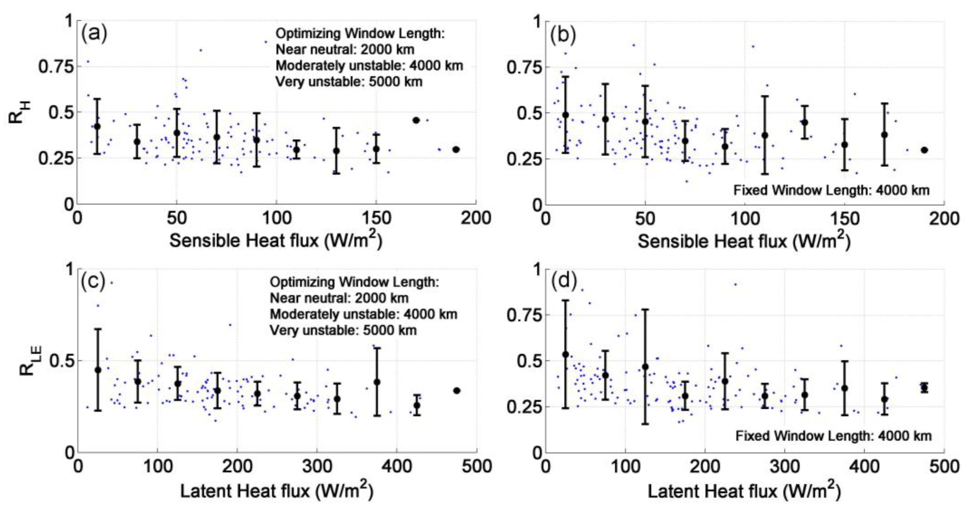
4.3. Evaluation of the Optimizing Window Length

We employed the optimizing window length to calculate the turbulent heat fluxes and to evaluate the performance of the optimizing window length. According to the results of Section 4.2, we chose the window lengths of 2 km for near neutral conditions, 4 km for moderately unstable conditions, and 5 km for very unstable conditions to calculate the turbulent heat fluxes and their relative uncertainties. Meanwhile, we also used a fixed 4 km window length to calculate the turbulent heat fluxes and their relative uncertainties to illustrate the inadequacy of applying a fixed window length for turbulent heat fluxes estimation without considering the atmospheric stability. Only high-quality turbulent heat fluxes results (overall quality flag between 1 and 6, according to Vellinga et al. [42]) were considered in the following analysis.

Theoretically, the window length for airborne flux measurements depends on the flying altitude, surface characteristics, and atmospheric stability [39]. In this study, we ignored the influence of flight height and surface features on the choice of window length, and only investigated the relationship between the window length and the atmospheric stability conditions. This is because the mixing process of turbulence between the land surface and the flight level makes the impact of surface characteristics on airborne EC measurements very complicated. In the following, we used the estimated turbulent heat fluxes as an approximation of averaged true surface heat fluxes (within the footprint area) to evaluate the performance of the optimizing window length under different surface heating status (Figure 10). In Figure 10, it is clear that the turbulent heat fluxes based on the optimizing window length have higher accuracy than the turbulent heat fluxes based on the fixed window length. We found that large relative uncertainties were present on the low flux magnitude domain (small than 30 Wm⁻² for both sensible and latent heat fluxes). In this study, the low flux conditions are associated with the near neutral atmospheric stability conditions, when the potential air temperature is near constant with height and the mechanical shear dominates the turbulence production. EC measurements under these conditions have poor accuracy in nature, and can easily be affected by heterogeneous turbulence. Nevertheless, our determined optimizing window length under the near neutral conditions could effectively avoid the influence of heterogeneous turbulence on the estimated turbulent heat fluxes and give relatively reliable flux estimates. With the increase of surface heat flux intensity, the development of turbulence was significantly enhanced, and the size of eddies associated with the local transport of heat fluxes increased as well. In particular, for the very unstable atmospheric stability conditions, where the large surface heat flux value often occurs (more than 100 Wm⁻² for sensible heat flux, and more than 200 Wm⁻² for latent heat flux in Figure 10), the large eddies dominate the transmission of energy. Our determined optimizing window length under the very unstable conditions also proved to give accurate and robust turbulent heat flux estimates. It illustrates that our defined optimizing window lengths are suitable for different heating conditions of the study area, and can give accurate and robust estimates of turbulent heat fluxes.

In addition, as the surface temperature represents the main driving force of thermal buoyancy, it has a great influence on the turbulent heat fluxes. If the estimated turbulent heat fluxes represent a great contribution from the local land surface, we could expect that the turbulent heat fluxes based on the optimizing window length have a better relationship with the local surface temperature than that based on a fixed window length. Figure 11 shows the relationships between the window-length averaged surface temperature (measured using an infrared thermometer) and the turbulent heat fluxes (sum of H and LE) based on the optimizing (Figure 11a) and fixed (Figure 11b) window lengths. The result from the optimized window length shows a better correlation between the turbulent heat fluxes and surface temperature. This implies that our defined optimizing window length and corresponding turbulent heat fluxes are consistent with the local surface features at window scale.

5. Discussion

The above results can confirm that our optimizing window lengths are characterized by both the surface features of the study area and the atmospheric stability conditions during the measurements. The main purpose of this study was to determine the optimum window length, which was used to separate the mesoscale motion influence of the turbulence and obtain more accurate turbulent heat flux estimates than those obtained using a fixed window length, which does not consider the atmospheric stability conditions. As the primary sources of atmospheric turbulence, the wind shear and buoyancy’s comprehensive effect can be described using the M–O similarity theory, which can be expressed as atmospheric stability. Therefore, this study attempts to give the optimizing window lengths for turbulent heat flux calculations that are suitable for near neutral to unstable atmospheric stability conditions. In this study, the results from the Ogive analysis provided the ranges of possible window lengths from the near neutral to very unstable conditions. The final determined optimum window lengths were determined after considering the accuracy, robustness, and local significance of the flux estimates. For the present study, we summarized the optimum window lengths under near neutral to unstable atmospheric stability conditions, as listed in

Table 5. The determined optimizing window lengths for turbulent heat fluxes calculation from airborne eddy covariance (EC) method under near neutral to unstable atmospheric stability conditions for the present study.

Atmospheric Stability Condition ($\mathsf{\zeta }$)	Optimum Window Length (m)
neutral conditions ($\left|\mathsf{\zeta }\right|\le 0.2$)	2000–2500
moderately unstable conditions ($-1\le \mathsf{\zeta }<-0.2$)	3900–5000
Very unstable conditions ($\mathsf{\zeta }<-1$)	4500–5000

, and discussed them in detail.

Under near neutral conditions, the turbulent mixing process is governed by mechanical shear (i.e., friction velocity), and the potential temperature is near constant with height. Under these conditions, the turbulent heat and moisture exchange near the surface is small, and EC measurements are vulnerable to exogenous influence (surface heterogeneity). This is a nonideal environment for EC measurements because of low flux conditions and weak vertical mixing. This is also the reason why the relative uncertainty of both the turbulent sensible and latent heat fluxes is large and scattered (upper panels in Figure 7). EC measurement under these conditions should be conducted cautiously. For such conditions, because the vertical gradient of potential temperature is close to zero, the vertical mixing of local turbulence is insufficient and any small-scaled surface heterogeneity could drastically influence the local turbulent heat fluxes [80]. A short window length is required to exclude the influence of small mesoscale turbulence; however, too short a window length may result in inadequate sampling with high uncertainty. In this study, we determined the final optimum window length based on the evolution of averaged relative uncertainty and its SD. From the top panels of Figure 6, we found that the general trend of averaged relative uncertainties is to first decline (at window lengths from 500 m to 2000 m) and then increase (at window lengths larger than 2500 m). At a window length of 2000 m, the averaged relative uncertainty started to be smaller than 0.5 for both the sensible and latent heat fluxes. For both the sensible and latent heat fluxes, the averaged relative uncertainty begins to be more than 0.5 at a window length of 2500 m. After the window lengths longer than 2500 m, the averaged relative uncertainty and its SD significantly begin to increase. So, we determined that the optimum lengths under the neutral conditions ranges from 2000 m to 2500 m. The fluctuation of relative uncertainty among the optimum window lengths is partly due to the relaxed stationarity test criteria we used in the preprocessing stage, and partly due to the sporadic buoyancy events that contribute to the turbulent heat fluxes (especially for sensible heat flux, Figure 7a) [30]. If we ignore the effects from sporadic events (maybe related to surface heterogeneity), then we can conclude that the optimum window lengths range from 2000 m to 2500 m, which can both exclude the negative influence from mesoscale turbulence and maintain the robustness of the turbulent heat flux estimates under the near neutral conditions.

The moderately unstable conditions represent the ideal EC measurement environment, when the air is heated from the bottom up (i.e., the surface heat flux is positive, as in the daytime over land) and the vertical mixing of turbulence is enhanced. Under these conditions, the turbulent mixing process is governed by both the wind shear and the buoyancy, and the typical scale of local turbulence is relative large. For these conditions, the influence of mesoscale turbulence is relatively small. From the top panels of Figure 8, the accuracy and robustness of turbulent heat flux estimates under these conditions are the best. We defined the optimizing window length under moderately unstable conditions in a relatively strict manner, that is, both the averaged relative uncertainty and its SD are stable and smaller than 0.5. After considering the variability of turbulent heat fluxes (bottom panels of Figure 8), we gave a relatively wide range of optimum window lengths (3900 m to 5000 m). This is because the mesoscale turbulence contains little energy under the moderately unstable conditions, so a longer window have less impact on the calculated turbulent heat fluxes. In addition, from the upper panels of Figure 8, the relative uncertainty of sensible heat flux is obviously smaller than that of latent heat flux. This is because the horizontal mixing of water vapor is more efficient than sensible heat flux, which reduces the relative influence of surface heterogeneity and increases the horizontal mixing scale of moisture. So, if the same window length is used to calculate the turbulent sensible and latent heat fluxes, the uncertainty of the latent heat flux will be greater than that of the sensible heat flux. If we want to obtain a latent heat flux with higher precision, a longer window length is needed. If we want to get more information about the surface heterogeneity, a relatively small window length is recommended.

Under very unstable atmospheric stability conditions, the turbulent mixing process is dominated by buoyancy, and influences of wind shear is negligible (the winds are calm or constant with height). For these conditions, the boundary layer is filled with large-scale eddies, and these large eddies dominate the transmission of energy. Under very unstable conditions, a particularly long window length is required to cover the large eddies with large energy transmission. If we choose an insufficient window length to calculate the turbulent heat fluxes, the turbulent heat fluxes will have low accuracy and be very unstable. This means that we cannot replicate the observed turbulent heat fluxes under the same region and similar surface and weather conditions, and it is the reason why the very large relative uncertainties occurred at window lengths less than 4500 m for sensible heat flux and less than 4100 m for latent heat flux in the upper panels of Figure 9. Again, in the upper panels of Figure 9, it is clear that with the increase of sampling length, the relative uncertainties and their SD decrease significantly. This is similar to the results of Lenschow et al. [19], who indicated that the longer the sampling interval was, the higher the accuracy of turbulent flux that could be obtained in convection boundary layer. However, our results indicated that an overlong window length can cause significant variability in the flux values (as indicated by the window lengths larger than 5000 m in the bottom panels in Figure 9) because they include the effect of mesoscale turbulence. So, combining the statistical error and variability of turbulent heat fluxes, we concluded that the optimum window lengths range from 4500 m to 5000 m for very unstable conditions. In the range of the defined optimum window lengths, sensible heat flux shows higher uncertainty than latent heat flux. This is because sensible heat flux, as an active scalar, has high vertical fluctuations along with the buoyancy term, so a longer window length is required to obtain a statistically significant value.

Airborne EC method is one of the most effective tools to provide turbulent flux measurements at a regional scale. One important application of airborne EC measurements is to provide the “true” surface flux values at the regional scale, which can be used to calibrate and validate process-oriented models in which land surface fluxes are linked to local surface exchange processes. So, the accuracy and the surface representativeness of turbulent flux estimates are the two main aspects that should be considered by the airborne EC measurements. This study indicates that the choice of window length for calculations of airborne turbulent heat fluxes should consider the atmospheric stability condition during the measurements. In particular, when conducting long-term airborne EC measurements, the present study presents a comprehensive methodology to find the optimum window lengths with which to compromise a balance between the accuracy and the surface representativeness of turbulent heat flux calculation.

6. Conclusions

The main purpose of this study was to find the optimum window length for heat flux calculation under near neutral to unstable atmospheric stability conditions, which is meaningful for depicting the flux contribution from local land surfaces. The results of the Ogive classification indicate that the reference window length of 2 km cannot capture a reliable estimate of the turbulent heat fluxes in any of the atmospheric stability conditions. Under moderately and very unstable conditions, the window length should be longer than 2 km, as it was found that divergent cases occupied the largest fraction of the Ogive cases. Under near neutral conditions, the reversed cases (including sign reversed and shape reversed cases) represented the biggest proportion in the Ogive cases. These reversed cases are caused by mesoscale turbulence motions associated with surface heterogeneity. Under near neutral conditions, turbulent heat fluxes are easily affected by heterogeneous turbulence due to the insufficient mixing of local turbulence. We found that the window length under neutral conditions should be smaller than the window length under moderate and very unstable conditions. With the development of instability from neutral to very unstable conditions, the mixing of local turbulent flux becomes more and more efficient. This reduces the impact of surface heterogeneity and increases the required window length to “catch” the flux contribution from large eddies.

The results from the Ogive analysis gave us reasonable information about the ranges of window lengths, which is significant to the fundamental assumptions behind the EC method. To understand the accuracy and the robustness of the flux estimates, the uncertainty analysis of flux was carried out to study the relationship between the flux uncertainty and the window length. We determined the optimum window length for near neutral to unstable atmospheric stability conditions after considering the accuracy, robustness, and local significance of the flux estimates. Under near neutral conditions, turbulent flux is vulnerable to exogenous influence (heterogeneous turbulence) due to the low flux conditions and weak vertical mixing. A short window length is required to exclude the impact from mesoscale turbulence. We found that the optimum window lengths range from 2000 m to 2500 m, which are capable of both removing the mesoscale influence and maintaining the reliability of turbulent heat flux estimates. From moderately to very unstable conditions, the mixing of local turbulent flux becomes more and more efficient and the size of eddies associated with the local fluxes increase notably. Under moderately unstable conditions, the turbulent mixing process is governed by both the wind shear and the buoyancy, and the influence of mesoscale turbulence is very small. We found that relatively broader window lengths ranging from 3900 m to 5000 m are optimum under moderately unstable conditions. Under very unstable conditions, the turbulent mixing process is dominated by the buoyancy, and the influence of wind shear is negligible. For these conditions, large convective eddies dominate the transmission of energy and a particularly long window length is required to cover the large eddies with large energy transmission. We found that window lengths ranging from 4500 m to 5000 m are optimum for producing turbulent heat fluxes with acceptable uncertainty. It is noted that the optimum window lengths should be region-specific. This study gives a comprehensive methodology to determine the optimizing window lengths in order to compromise to a balance between the accuracy and the surface representativeness of turbulent heat fluxes calculation. The turbulent heat fluxes calculated based on the optimum window lengths are not only meaningful in local land surface, but also have better accuracy. Finally, we conclude that the aircraft-based EC method for calculating turbulent heat fluxes should be used with varying window lengths that should be determined according to the atmospheric stability conditions.

References

1. Chen, J.M.; Leblanc, S.G.; Cihlar, J. Extending aircraft- and tower-based CO2 flux measurements to a boreal region using a landsat thematic mapper land cover map. J. Geophys. Res. Atmos. 1999, 104, 16859–16877. [Google Scholar] [CrossRef]
2. Desjardins, R.L.; MacPherson, J.I.; Mahrt, L.; Schuepp, P.; Pattey, E.; Neumann, H.; Baldocchi, D.; Wofsy, S.; Fitzjarrald, D.; McCaughey, H.; et al. Scaling up flux measurements for the boreal forest using aircraft-tower combinations. J. Geophys. Res. Atmos. 1997, 102, 29125–29133. [Google Scholar] [CrossRef]
3. Horst, T.W.; Weil, J.C. Footprint estimation for scalar flux measurements in the atmospheric surface layer. Bound.-Layer Meteorol. 1992, 59, 279–296. [Google Scholar] [CrossRef]
4. Saac, P.R.; McAneney, J.; Leuning, R.; Hacker, J.M. Comparison of aircraft and ground-based flux measurements during Oasis95. Bound.-Layer Meteorol. 2004, 110, 39–67. [Google Scholar]
5. Bertoldi, G.; Kustas, W.P.; Albertson, J.D. Evaluating source area contributions from aircraft flux measurements over heterogeneous land using large-eddy simulation. Bound.-Layer Meteorol. 2013, 147, 261–279. [Google Scholar] [CrossRef]
6. Metzger, S.; Junkermann, W.; Mauder, M.; Butterbach-Bahl, K.; Widemann, B.T.; Neidl, F.; Schafer, K.; Wieneke, S.; Zheng, X.H.; Schmid, H.P.; et al. Spatially explicit regionalization of airborne flux measurements using environmental response functions. Biogeosciences 2013, 10, 2193–2217. [Google Scholar] [CrossRef] [Green Version]
7. Baldocchi, D.D.; Hincks, B.B.; Meyers, T.P. Measuring biosphere-atmosphere exchanges of biologically related gases with micrometeorological methods. Ecology 1988, 69, 1331–1340. [Google Scholar] [CrossRef]
8. Foken, T.; Aubinet, M.; Leuning, R. The eddy covariance method. In Eddy Covariance: A Practical Guide to Measurement and Data Analysis; Aubinet, M., Vesala, T., Papale, D., Eds.; Springer Netherlands: Dordrecht, The Nederlands, 2012; pp. 1–19. [Google Scholar]
9. Foken, T.; Wichura, B. Tools for quality assessment of surface-based flux measurements. Agric. For. Meteorol. 1996, 78, 83–105. [Google Scholar] [CrossRef]
10. Finnigan, J.J.; Clement, R.; Malhi, Y.; Leuning, R.; Cleugh, H.A. A re-evaluation of long-term flux measurement techniques—Part I: Averaging and coordinate rotation. Bound.-Layer Meteorol. 2003, 107, 1–48. [Google Scholar] [CrossRef]
11. Lee, X.; Massman, W.; Law, B. Handbook of Micrometeorology; Kluwer Academic Publishers: Dordrecht, The Netherlands, 2004; pp. 7–238. [Google Scholar]
12. Foken, T.; Wimmer, F.; Mauder, M.; Thomas, C.; Liebethal, C. Some aspects of the energy balance closure problem. Atmos. Chem. Phys. 2006, 6, 4395–4402. [Google Scholar] [CrossRef]
13. Mahrt, L.; Macpherson, J.I.; Desjardins, R. Observations of fluxes over heterogeneous surfaces. Bound.-Layer Meteorol. 1994, 67, 345–367. [Google Scholar] [CrossRef]
14. Mitic, C.M.; Schuepp, P.H.; Desjardins, R.L.; Macpherson, I.J. Flux association in coherent structures transporting CO2, H2O, heat and ozone over the code grid site. Agric. For. Meteorol. 1997, 87, 27–39. [Google Scholar] [CrossRef]
15. Aubinet, M. Eddy covariance CO2 flux measurements in nocturnal conditions: An analysis of the problem. Ecol. Appl. 2008, 18, 1368–1378. [Google Scholar] [CrossRef] [PubMed]
16. Von Randow, C.; Sa, L.D.A.; Gannabathula, P.; Manzi, A.O.; Arlino, P.R.A.; Kruijt, B. Scale variability of atmospheric surface layer fluxes of energy and carbon over a tropical rain forest in southwest amazonia-1. Diurnal conditions. J. Geophys. Res.-Atmos. 2002, 107. [Google Scholar] [CrossRef]
17. Sievers, J.; Papakyriakou, T.; Larsen, S.E.; Jammet, M.M.; Rysgaard, S.; Sejr, M.K.; Sørensen, L.L. Estimating surface fluxes using eddy covariance and numerical ogive optimization. Atmos. Chem. Phys. 2015, 15, 2081–2103. [Google Scholar] [CrossRef] [Green Version]
18. Sun, X.M.; Zhu, Z.L.; Wen, X.F.; Yuan, G.F.; Yu, G.R. The impact of averaging period on eddy fluxes observed at chinaflux sites. Agric. For. Meteorol. 2006, 137, 188–193. [Google Scholar] [CrossRef]
19. Lenschow, D.H.; Mann, J.; Kristensen, L. How long is long enough when measuring fluxes and other turbulence statistics. J. Atmos. Ocean. Technol. 1994, 11, 661–673. [Google Scholar] [CrossRef]
20. Lemone, M.A.; Grossman, R.L.; Chen, F.; Lkeda, K.; Yates, D.N. Choosing the averaging interval for comparison of observed and modeled fluxes along aircraft transects over a heterogeneous surface. J. Hydrometeorol. 2003, 2, 179–195. [Google Scholar] [CrossRef]
21. Lenschow, D.H.; Stankov, B.B. Length scales in the convective boundary layer. J. Atmos. Sci. 1986, 43, 1198–1209. [Google Scholar] [CrossRef]
22. Mauder, M.; Desjardins, R.L.; MacPherson, I. Scale analysis of airborne flux measurements over heterogeneous terrain in a boreal ecosystem. J. Geophys. Res. 2007, D13112, 1–13. [Google Scholar] [CrossRef]
23. Charuchittipan, D.; Babel, W.; Mauder, M.; Leps, J.-P.; Foken, T. Extension of the averaging time in eddy-covariance measurements and its effect on the energy balance closure. Bound.-Layer Meteorol. 2014, 152, 303–327. [Google Scholar] [CrossRef]
24. Grossman, R.L. Sampling errors in the vertical fluxes of potential temperature and moisturemeasured by aircraft during fife. J. Geophys. Res. 1992, 97, 18439–18443. [Google Scholar] [CrossRef]
25. Crawford, T.L.; McMillen, R.T.; Dobosy, R.J.; Macpherson, I. Correcting airborne flux measurements for aircraft speed variation. Bound.-Layer Meteorol. 1993, 66, 237–245. [Google Scholar] [CrossRef]
26. Mauder, M.; Desjardins, R.L.; MacPherson, I. Creating surface flux maps from airborne measurements: Application to the Mackenzie area Gewex study Mags 1999. Bound.-Layer Meteorol. 2008, 129, 431–450. [Google Scholar] [CrossRef]
27. Kirby, S.; Dobosy, R.; Williamson, D.; Dumas, E. An aircraft-based data analysis method for discerning individual fluxes in a heterogeneous agricultural landscape. Agric. For. Meteorol. 2008, 148, 481–489. [Google Scholar] [CrossRef]
28. Beyrich, F.; Leps, J.P.; Mauder, M.; Bange, J.; Foken, T.; Huneke, S.; Lohse, H.; Lüdi, A.; Meijninger, W.M.L.; Mironov, D. Area-averaged surface fluxes over the litfass region based on eddy-covariance measurements. Bound.-Layer Meteorol. 2006, 121, 33–65. [Google Scholar] [CrossRef]
29. Vickers, D.; Mahrt, L. Quality control and flux sampling problems for tower and aircraft data. J. Atmos. Ocean. Technol. 1997, 14, 512–526. [Google Scholar]
30. Mahrt, L. Computing turbulent fluxes near the surface: Needed improvements. Agric. For. Meteorol. 2010, 150, 501–509. [Google Scholar] [CrossRef]
31. Gioli, B.; Miglietta, F.; Vaccari, F.P.; Zaldei, A.; Martino, B.D. The sky arrow era, an innovative airborne platform to monitor mass, momentum and energy exchange of ecosystems. Ann. Geophys. 2006, 49, 109–116. [Google Scholar]
32. Michels, B.I.; Jochum, A.M. Heat and moisture flux profiles in a region with inhomogeneous surface evaporation. J. Hydrol. 1995, 166, 383–407. [Google Scholar] [CrossRef]
33. Brasa-Ramos, A.; de Santa Olalla, F.M.I.; Caselles, V.; Jochum, A.M. Comparison of evapotranspiration estimates by noaa-avhrr images and aircraft flux measurements in a semiarid region of Spain. J. Agric. Eng. Res. 1998, 70, 285–294. [Google Scholar] [CrossRef]
34. Bange, J.; Zittel, P.; Spieß, T.; Uhlenbrock, J.; Beyrich, F. A new method for the determination of area-averaged turbulent surface fluxes from low-level flights using inverse models. Bound.-Layer Meteorol. 2006, 119, 527–561. [Google Scholar] [CrossRef]
35. Friehe, C.A.; Shaw, W.J.; Rogers, D.P.; Davidson, K.L.; Large, W.G.; Stage, S.A.; Crescenti, G.H.; Khalsa, S.J.S.; Greenhut, G.K.; Li, F. Air-sea fluxes and surface layer turbulence around a sea surface temperature front. J. Geophys. Res. Oceans 1991, 96, 8593–8609. [Google Scholar] [CrossRef]
36. Bange, J.; Beyrich, F.; Engelbart, D.A.M. Airborne measurements of turbulent fluxes during litfass-98: Comparison with ground measurements and remote sensing in a case study. Theor. Appl. Climatol. 2002, 73, 35–51. [Google Scholar] [CrossRef]
37. Foken, T. Experimental methods for estimating the fluxes of energy and matter. In Micrometeorology; Springer: Berlin/Heidelberg, Germany, 2008; pp. 105–151. [Google Scholar]
38. Desjardins, R.L.; MacPherson, J.I.; Schuepp, P.H.; Karanja, F. An evaluation of aircraft flux measurements of CO2, water vapor and sensible heat. Bound.-Layer Meteorol. 1989, 47, 55–69. [Google Scholar] [CrossRef]
39. Gioli, B.; Miglietta, F.; De Martino, B.; Hutjes, R.W.A.; Dolman, H.A.J.; Lindroth, A.; Schumacher, M.; Sanz, M.J.; Manca, G.; Peressotti, A.; et al. Comparison between tower and aircraft-based eddy covariance fluxes in five european regions. Agric. For. Meteorol. 2004, 127, 1–16. [Google Scholar] [CrossRef]
40. Hutjes, R.W.A.; Vellinga, U.S.; Gioli, B.; Miglietta, F. Dis-aggregation of airborne flux measurements using footprint analysis. Agric. For. Meteorol. 2010, 150, 966–983. [Google Scholar] [CrossRef]
41. Ogunjemiyo, S.O.; Kaharabata, S.K.; Schuepp, P.H.; MacPherson, I.J.; Desjardins, R.L.; Roberts, D.A. Methods of estimating CO2, latent heat and sensible heat fluxes from estimates of land cover fractions in the flux footprint. Agric. For. Meteorol. 2003, 117, 125–144. [Google Scholar] [CrossRef]
42. Vellinga, O.S.; Dobosy, R.J.; Dumas, E.J.; Gioli, B.; Elbers, J.A.; Hutjes, R.W.A. Calibration and quality assurance of flux observations from a small research aircraft. J. Atmos. Ocean. Technol. 2013, 30, 161–181. [Google Scholar] [CrossRef]
43. Miglietta, F.; Gioli, B.; Brunet, Y.; Hutjes, R.W.A.; Matese, A.; Sarrat, C.; Zaldei, A. Sensible and latent heat flux from radiometric surface temperatures at the regional scale: Methodology and evaluation. Biogeosciences 2009, 6, 1975–1986. [Google Scholar] [CrossRef]
44. Vellinga, O.S.; Gioli, B.; Elbers, J.A.; Holtslag, A.A.M.; Kabat, P.; Hutjes, R.W.A. Regional carbon dioxide and energy fluxes from airborne observations using flight-path segmentation based on landscape characteristics. Biogeosciences 2010, 7, 1307–1321. [Google Scholar] [CrossRef]
45. Isaac, P.R.; Leuning, R.; Hacker, J.M.; Cleugh, H.A.; Coppin, P.A.; Denmead, O.T.; Raupach, M.R. Estimation of regional evapotranspiration by combining aircraft and ground-based measurements. Bound.-Layer Meteorol. 2004, 110, 69–98. [Google Scholar] [CrossRef]
46. Lothon, M.; Couvreux, F.; Donier, S.; Guichard, F.; Lacarrère, P.; Lenschow, D.H.; Noilhan, J.; Saïd, F. Impact of coherent eddies on airborne measurements of vertical turbulent fluxes. Bound.-Layer Meteorol. 2007, 124, 425–447. [Google Scholar] [CrossRef]
47. Caramori, P.; Schuepp, P.H.; Desjardins, R.L.; Macpherson, J.I. Structural analysis of airborne flux estimates over a region. J. Clim. 1994, 7, 627–640. [Google Scholar] [CrossRef]
48. Lemone, M.A.; Grossman, R.L.; McMillen, R.T.; Liou, K.-N.; Ou, S.C.; McKeen, S.; Angevine, W.; Ikeda, K.; Chen, F. Cases-97: Late-morning warming and moistening of the convective boundary layer over the walnut river watershed. Bound.-Layer Meteorol. 2002, 104, 1–52. [Google Scholar] [CrossRef]
49. Hutjes, R.; Vellinga, O.; Elbers, J. Using aircraft observations to characterise the full seasonal dynamics of evaporation and carbon dioxide fluxes from heterogeneous landscapes in The Netherlands. In Proceedings of the EGU General Assembly Conference, Vienna, Austria, 7–12 April 2013; Volume 15. [Google Scholar]
50. Meesters, A.; Tolk, L.F.; Peters, W.; Hutjes, R.W.A.; Vellinga, O.S.; Elbers, J.A.; Vermeulen, A.T.; van der Laan, S.; Neubert, R.E.M.; Meijer, H.A.J.; et al. Inverse carbon dioxide flux estimates for The Netherlands. J. Geophys. Res.-Atmos. 2012, 117. [Google Scholar] [CrossRef]
51. Hacker, J.; Crawford, T. The bat-probe: The ultimate tool to measure turbulence from any kind of aircraft (or sailplane). Tech. Soar. 1999, 2, 42–45. [Google Scholar]
52. Dumas, E.J.; Brooks, S.B.; Verfaillie, J. Development and testing of a sky arrow 650 era for atmospheric research. In Proceedings of the 11th Symposium on Meteorological Observations and Instrumentation, Albuquerque, NM, USA, 14–18 January 2001; pp. 129–133. [Google Scholar]
53. Hazeu, G.W.; Bregt, A.K.; de Wit, A.J.W.; Clevers, J. A Dutch multi-date land use database: Identification of real and methodological changes. Int. J. Appl. Earth Obs. Geoinf. 2011, 13, 682–689. [Google Scholar] [CrossRef]
54. Raupach, M.R.; Finnigan, J.J. Scale issues in boundary-layer meteorology-surface-energy balances in heterogeneous terrain. Hydrol. Process. 1995, 9, 589–612. [Google Scholar] [CrossRef]
55. Grunwald, J.; Kalthoff, N.; Corsmeier, U.; Fiedler, E. Comparison of areally averaged turbulent fluxes over non-homogeneous terrain: Results from the efeda-field experiment. Bound.-Layer Meteorol. 1996, 77, 105–134. [Google Scholar] [CrossRef]
56. Foken, T. 50 years of the monin–obukhov similarity theory. Bound.-Layer Meteorol. 2006, 119, 431–447. [Google Scholar] [CrossRef]
57. Businger, J.A.; Wyngaard, J.C.; Izumi, Y.; Bradley, E.F. Flux-profile relationships in the atmospheric surface layer. J. Atmos. Sci. 1971, 28, 181–189. [Google Scholar] [CrossRef]
58. Kaimal, J.C.; Clifford, S.F.; Lataitis, R.J. Effect of finite sampling on atmospheric spectra. Bound.-Layer Meteorol. 1989, 47, 337–347. [Google Scholar] [CrossRef]
59. Lenschow, D.H.; Sun, J.L. The spectral composition of fluxes and variances over land and sea out to the mesoscale. Bound.-Layer Meteorol. 2007, 125, 63–84. [Google Scholar] [CrossRef]
60. Stull, R.B. Some mathematical & conceptual tools: Part 1. Statistics. In An Introduction to Boundary Layer Meteorology; Stull, R.B., Ed.; Springer: Dordrecht, The Nederlands, 1988; pp. 29–74. [Google Scholar]
61. Berger, B.W.; Davis, K.J.; Yi, C.X.; Bakwin, P.S.; Zhao, C.L. Long-term carbon dioxide fluxes from a very tall tower in a northern forest: Flux measurement methodology. J. Atmos. Ocean. Technol. 2001, 18, 529–542. [Google Scholar] [CrossRef]
62. Mauder, M.; Cuntz, M.; Drue, C.; Graf, A.; Rebmann, C.; Schmid, H.P.; Schmidt, M.; Steinbrecher, R. A strategy for quality and uncertainty assessment of long-term eddy-covariance measurements. Agric. For. Meteorol. 2013, 169, 122–135. [Google Scholar] [CrossRef]
63. Mahrt, L. Flux sampling errors for aircraft and towers. J. Atmos. Ocean. Technol. 1998, 15, 416–429. [Google Scholar] [CrossRef]
64. Betts, A.K.; Desjardins, R.L.; Macpherson, J.I.; Kelly, R.D. Boundary-layer heat and moisture budgets from fife. Bound.-Layer Meteorol. 1990, 50, 109–138. [Google Scholar] [CrossRef]
65. Lemone, M.A.; Chen, F.; Alfieri, J.G.; Tewari, M.; Geerts, B.; Miao, Q.; Grossman, R.L.; Coulter, R.L. Influence of land cover and soil moisture on the horizontal distribution of sensible and latent heat fluxes in southeast kansas during ihop_2002 and cases-97. J. Hydrometeorol. 2006, 8, 68–87. [Google Scholar] [CrossRef]
66. Billesbach, D.P. Estimating uncertainties in individual eddy covariance flux measurements: A comparison of methods and a proposed new method. Agric. For. Meteorol. 2011, 151, 394–405. [Google Scholar] [CrossRef]
67. Finkelstein, P.L.; Sims, P.F. Sampling error in eddy correlation flux measurements. J. Geophys. Res.-Atmos. 2001, 106, 3503–3509. [Google Scholar] [CrossRef]
68. Sun, J.L.; Howell, J.F.; Esbensen, S.K.; Mahrt, L.; Greb, C.M.; Grossman, R.; LeMone, M.A. Scale dependence of air-sea fluxes over the western equatorial pacific. J. Atmos. Sci. 1996, 53, 2997–3012. [Google Scholar] [CrossRef]
69. Sakai, R.K.; Fitzjarrald, D.R.; Moore, K.E. Importance of low-frequency contributions to eddy fluxes observed over rough surfaces. J. Appl. Meteorol. 2001, 40, 2178–2192. [Google Scholar] [CrossRef]
70. Albertson, J.D.; Parlange, M.B. Natural integration of scalar fluxes from complex terrain. Adv. Water Resour. 1999, 23, 239–252. [Google Scholar] [CrossRef]
71. Kustas, W.P.; Anderson, M.C.; French, A.N.; Vickers, D. Using a remote sensing field experiment to investigate flux-footprint relations and flux sampling distributions for tower and aircraft-based observations. Adv. Water Resour. 2006, 29, 355–368. [Google Scholar] [CrossRef]
72. Mahrt, L.; Vickers, D.; Sun, J.L. Spatial variations of surface moisture flux from aircraft data. Adv. Water Resour. 2001, 24, 1133–1141. [Google Scholar] [CrossRef]
73. Kaimal, J.C.; Wyngaard, J.C.; Izumi, Y.; Coté, O.R. Spectral characteristics of surface-layer turbulence. Q. J. R. Meteorol. Soc. 1972, 98, 563–589. [Google Scholar] [CrossRef]
74. Olesen, H.R.; Larsen, S.E.; Hojstrup, J. Modeling velocity spectra in the lower part of the planetary boundary-layer. Bound.-Layer Meteorol. 1984, 29, 285–312. [Google Scholar] [CrossRef]
75. Hojstrup, J. Velocity spectra in the unstable planetary boundary-layer. J. Atmos. Sci. 1982, 39, 2239–2248. [Google Scholar] [CrossRef]
76. Wyngaard, J.C. Turbulence in the Atmosphere; Cambridge University Press: Cambridge, UK, 2010. [Google Scholar]
77. Van den Kroonenberg, A.; Bange, J. Turbulent flux calculation in the polar stable boundary layer: Multiresolution flux decomposition and wavelet analysis. J. Geophys. Res.-Atmos. 2007, 112. [Google Scholar] [CrossRef]
78. Cheng, W.C.; Liu, C.H. Large-eddy simulation of turbulent transports in urban street canyons in different thermal stabilities. J. Wind Eng. Ind. Aerodyn. 2011, 99, 434–442. [Google Scholar] [CrossRef]
79. Bertoldi, G.; Kustas, W.P.; Albertson, J.D. Estimating spatial variability in atmospheric properties over remotely sensed land surface conditions. J. Appl. Meteorol. Climatol. 2008, 47, 2147–2165. [Google Scholar] [CrossRef]
80. Vickers, D.; Mahrt, L. The cospectral gap and turbulent flux calculations. J. Atmos. Ocean. Technol. 2003, 20, 660–672. [Google Scholar] [CrossRef]
81. Webb, E.K.; Pearman, G.I.; RG, L. Correction of flux measurements for density effects due to heat and water-vapor transfer. Q. J. R. Meteorol. Soc. 1980, 106, 85–100. [Google Scholar] [CrossRef]
82. Kaimal, J.C.; Finnigan, J.J. Atmospheric Boundary Layer Flows: Their Structure and Measurement; Oxford University Press: New York, NY, USA, 1994. [Google Scholar]
Figure 1. Land-use map of the study areas (between 4.69–5.21°E and 51.83–52.28°N) located in the west of the Netherlands and the flight patterns (black tracks) during the 2008.
Remotesensing 10 00670 g001
Figure 2. Diagram of the methodological framework of this study.
Remotesensing 10 00670 g002
Figure 3. The example diagram of Equation (4) for normal Ogive case (a) and extreme Ogive cases with strong influence from low-wavenumber component of turbulence (b).
Remotesensing 10 00670 g003
Figure 4. Normalized Ogives (gray lines) of sensible ( Og ^ Tw , ae) and latent ( Og ^ qw , fj) heat fluxes as a function of wavenumber. For both the top and bottom panels: from left to right correspond to the convergent (a,f), divergent (b,g), inadequate (c,h), sign reversal (d,I), and shape reversal (e,j) cases, respectively. The vertical black solid line indicates the wavenumber whose inverse yields a length of 2 km reference window length. The blue solid curves represent the typical shape corresponding to the respective Ogive category.
Remotesensing 10 00670 g004
Figure 5. The frequency histograms of the wavelength ( L meso ) at which the sign reversal occurred for sensible heat flux: (a) under near neutral conditions and (b) under moderately unstable and very unstable conditions. Wavelength interval for frequency histogram is 500 m.
Remotesensing 10 00670 g005
Figure 6. The frequency histograms of the wavelength ( L meso ) at which the sign reversal occurred for latent heat flux: (a) under near neutral conditions and (b) under moderately unstable and very unstable conditions. Wavelength interval for frequency histogram is 500 m.
Remotesensing 10 00670 g006
Figure 7. Averaged relative flux uncertainties ( R H ,   R LE ) with standard deviation (top panels) and block ensemble averaged non-dimensional flux ( E H ,   E LE ) (bottom panels) for sensible heat flux (a) and latent heat flux (b) under neutral conditions. In the bottom panel, the solid blue curves represent the median value, while the solid green lines depict the 10th (lower) and 90th (upper) percentiles.
Remotesensing 10 00670 g007
Figure 8. Averaged relative flux uncertainties ( R H ,   R LE ) with standard deviation (top panels) and block ensemble averaged non-dimensional flux ( E H ,   E LE ) (bottom panels) for sensible heat flux (a) and latent heat flux (b) under moderately unstable conditions. In the bottom panel, the solid blue curves represent the median value, while the solid green lines depict the 10th (lower) and 90th (upper) percentiles.
Remotesensing 10 00670 g008
Figure 9. Averaged relative flux uncertainties ( R H ,   R LE ) with standard deviation (top panels) and block ensemble averaged non-dimensional flux ( E H ,   E LE ) (bottom panels) for sensible heat flux (a) and latent heat flux (b) under very unstable conditions. In the bottom panel, the solid blue curves represent the median value, while the solid green lines depict the 10th (lower) and 90th (upper) percentiles.
Remotesensing 10 00670 g009
Figure 10. The relationship between the magnitude of heat fluxes and the relative flux uncertainties for sensible heat flux ( R H ; a,b) and latent heat flux ( R LE ; c,d) based on optimizing (a,c) and fixed (b,d) window length. The black error bars show the mean (dark spot) plus/minus one standard deviation (horizontal bars) of relative flux uncertainty for 10 evenly spaced bins of flux magnitude.
Remotesensing 10 00670 g010
Figure 11. The relationship between the surface temperature (K) and the turbulent heat flux (sum of H and LE) based on optimizing (a) and fixed (b) window length.
Remotesensing 10 00670 g011