Global MODIS Fraction of Green Vegetation Cover for Monitoring Abrupt and Gradual Vegetation Changes

Abstract

The presence and distribution of green vegetation cover in the biosphere are of paramount importance in investigating cause-effect phenomena at the land/atmosphere interface, estimating primary production rates as part of global carbon and water cycle assessments and evaluating soil protection and land use change over time. The fraction of green vegetation cover (FCover) as estimated from satellite observations has already been demonstrated to be an extraordinarily useful product for understanding vegetation cover changes, for supporting ecosystem service assessments over areas with variable extents and for processes spanning a variable period of time (abrupt events or long-term processes). This study describes a methodology implemented to estimate global FCover (from 2001 to 2015) by applying a linear spectral mixture analysis with global endmembers to an entire temporal series of MODIS satellite observations and gap-filling missing FCover observations in temporal series using the DINEOF algorithm. The resulting global MODV1 FCover product was validated with two global validation datasets and showed an overall good thematic absolute accuracy (RMSE = 0.146) consistent with the validation performance of other FCover global products. Basic statistics performed on the product show changes in average and trend values and allow for the quantification of gross vegetation loss and gain over different temporal scales. To demonstrate the capacity of this global product to monitor specific dynamics, a multitemporal analysis was performed on selected sites and vegetation responses (i.e., cover changes), and specific dynamics resulting from cause-effect phenomena are briefly discussed. The product is intended to be used for monitoring vegetation dynamics, but it also has the potential to be integrated in other modeling frameworks (e.g., the carbon cycle, primary production, and soil erosion) in conjunction with other spatial datasets such as those on climate and soil type.

1. Introduction

1.1. Importance of Greenness Mapping and Monitoring

The assessment of biodiversity, ecosystems and the services they provide requires a large number of dynamic inputs that translate global realities into measurable products. In terrestrial ecosystems, vegetation cover is a critical biodiversity variable [1] for the quantitative assessment of process-based models (e.g., soil erosion [2]).

Photosynthetic green vegetation (grassland, forest, cropland, etc.) and its functions, in addition to providing raw materials and other resources and being a biodiversity sink, contribute to the delivery of many ecosystem services related, for example, to soil protection, air and water quality, carbon storage, and climate change adaptation and mitigation [3].

These phenomena, which can be natural (e.g., severe drought and pests) or manmade (fires, deforestation, and urbanization), may have significant local as well as global ecological, socio-cultural and economic impacts. On the other hand, policies (e.g., mitigation actions within the UNFCCC policies and policy for turning brownfields into green space [4]), planning strategies (e.g., green infrastructure and networks [5]) and natural processes combined with human-induced ones [6] can also lead to an increase in vegetation cover.

To fulfill the need for the continuous monitoring of green cover over a wide range of temporal and spatial scales, satellite remote sensing (RS) represents a valuable source of information, especially for global and decadal assessments. Several vegetation indexes and biophysical variables derived from RS have been developed in recent decades, and many advances in analytical methodologies have been made to overcome RS data limitations, such as missing data.

1.2. Earth Observation Vegetation Monitoring

In general, terms, Earth observation (EO)-derived vegetation indexes are useful for decoupling vegetation and soil in energy balance processes [7], estimating soil erosion prevention [8,9], understanding biodiversity dynamics [10,11] and evaluating ecosystem responses to specific processes [12,13].

In recent years, vegetation indicators assessed from EO products have moved from spectral indexes, such as the normalized difference vegetation index (NDVI) [14], to biophysical variable estimates such as the leaf area index (LAI) [15], fraction of absorbed photosynthetically active radiation (absorbed by the photosynthesizing tissue in a canopy) (FAPAR) [16] and fraction of green vegetation cover (FCover) [15].

The international scientific community and a large range of users have included LAI, FAPAR and FCover among the BioPar (biophysical products) vegetation variables required for operational mapping products such as those provided by the European Copernicus Global Land Service. At the same time, although these measurements are not yet fully identified as essential biodiversity variables by biodiversity communities, initiatives such as GEOBON already recognize their usefulness and importance [17].

The BioPar user requirements document [18] collects the needs expressed by users and science communities about the EO derived bio-geophysical products and provides indications for the target relative and absolute accuracy thresholds and resolution, frequency and time span (i.e., 1 km spatial sampling and a 10-day frequency over a time period as long as possible).

Although LAI has been largely preferred in recent years for vegetation monitoring, it has been demonstrated that LAI tends to saturate at high values of density and cover, probably due to the reflectance saturation effect [7,19] and leaf clumping [20]. FAPAR, on the other hand, being sensitive to background reflectance, clump leaf area index, and atmospheric and bi-directional effects [16] can underestimate green cover values, compromising the knowledge of primary production functions.

In this context, FCover (also known as “FVC”) is a continuous variable corresponding to the green vegetation fraction covering a unit ground area as seen from the nadir direction. FCover depends on the canopy structural attributes, mainly leaf area index, leaf angle distribution, and clumping [7], and does not depend on the geometry of illumination, in contrast to FAPAR. FCover gives information about vegetation pixel purity and can be tailored to specific applications, especially if distributed as a systematically available global product [21]. Given these assumptions, the information provided by FCover complements LAI and FAPAR biophysical vegetation estimates and therefore plays a key role as a vegetation descriptor in combination with classical vegetation indexes.

FCover has already been estimated from EO data at the global scale, together with LAI and FAPAR retrievals, from the VEGETATION sensor aboard the SPOT satellites for the period 1999–2007 within the CYCLOPES project (CYCV31 product) [22] and aboard the PROBA-V satellite for the period 2013–2017 within the Copernicus Land Monitoring Service (GEOV1 product) [23]. The abovementioned products were validated using global land product validation datasets [24,25]. On the other hand, FCover estimations from the MODIS sensor (Moderate-resolution Imaging Spectroradiometer) aboard the Terra satellite are not included among the vegetation products (e.g., MOD15A2, MOD13A3) distributed in the MODIS collection, which contains only LAI and FAPAR [26,27].

A MODIS product containing information analogous to FCover is the MOD44B, which provides the vegetation continuous field (VCF), is generated with a yearly temporal granularity and represents the percent of tree cover, percent of non-tree cover and percent of non-vegetated areas within each pixel. The MODIS data offer systematic acquisitions over the entire globe with a daily revisit time, ensuring a higher probability of cloud-free observations in monthly composites than SPOT VEGETATION acquisitions (a 10-day revisit time) over an extended period of time (2000–2017). The higher MODIS revisit time allows for wider multitemporal analysis, representing an advantage with respect to PROBA-V products, which have a comparable revisit time but limited availability (2013–2017).

1.3. Overcoming Earth Observation Data Constraints for a Global FCover Product

Optical remote sensing data are heavily hampered by clouds; therefore, most RS data processing algorithms perform cloud detection to remove pixels covered by clouds. Likewise, there are many other problems related to optical RS data acquisition that may affect data availability.

Missing data in multitemporal series of EO products over land and oceans lead to gappy data availability and represent a limitation for time series analysis and for many analytical tools used in the retrieval of temporal trend analysis in addition to signal noise. Many methodologies have been developed to overcome temporal gaps and noise in temporal series. Some examples of multitemporal series gap-filling and filtering are polynomial functions, such as spline interpolation [28] and the adaptive Savitzky-Golay filter [29]; asymmetrical Gaussian fitting [30]; smoothing techniques such as the Whittaker smoother [31,32]; spatio-temporal filters [33]; data interpolating empirical orthogonal functions (DINEOF) [34]; and linear quantile-regression on spatio-temporal subsets [35]. With the aim of generating an FCover product representing vegetation estimates with as few missing values as possible, a gap-filling procedure should preferably adopt a methodology that does not depend on time series smoothing to prevent abrupt changes within the time series from being flattened, thus limiting the detection of breaks in trend and seasonal components.

1.4. Study Objectives

The availability of a gap-filled global FCover product can support the continuous monitoring of green vegetation cover and provide quantitative information for the analysis of natural and manmade phenomena such as climate change, fire regimes, deforestation, soil erosion, and urbanization. Moreover, such a product can be assimilated in environmental models, such as those for the estimation of ecosystem services.

In consideration of the abovementioned issues, the aim of this study is to describe a new gap-filled FCover product (MODV1) generated by developing a specific processing chain based on well-known methodologies applied to MODIS data for long time series analysis. Basic statistics are computed from the resulting time series to give an overview of the new product in terms of the global distribution of green vegetation cover and the main global trends. In addition, to demonstrate the suitability of the product in monitoring green vegetation cover changes related to slow or abrupt processes, examples for selected sites are provided, and cause-effect phenomena are briefly discussed in terms of vegetation gain and loss dynamics.

2. Materials and Methods

2.1. Earth Observation Data

The MOD13A3 collection 6 provided by Land Processes Distributed Active Archive Center (LP DAAC) (https://lpdaac.usgs.gov/dataset_discovery/modis/modis_products_table/mod13a3_v006) [28], acquired by the MODIS optical multispectral sensor aboard the NASA Terra satellite over a 15-year period (2000–2015), was used to generate the FCover product at a global scale. The MOD13A3 product provides monthly composites of surface reflectance data corresponding to the blue (469 nm), red (645 nm), near-infrared (858.5 nm) and mid-infrared (2130 nm) spectral wavelengths gridded in the sinusoidal projection at a 1-km spatial resolution. MOD13A3 collection 6 contains significant revisions to the calibration approach to account for sensor degradation [36]. This monthly product is the result of the elaboration of all 16-day 1-km products that overlap within the month by applying a weighted temporal average if the pixel is cloud free or the maximum value in case the pixel contains clouds.

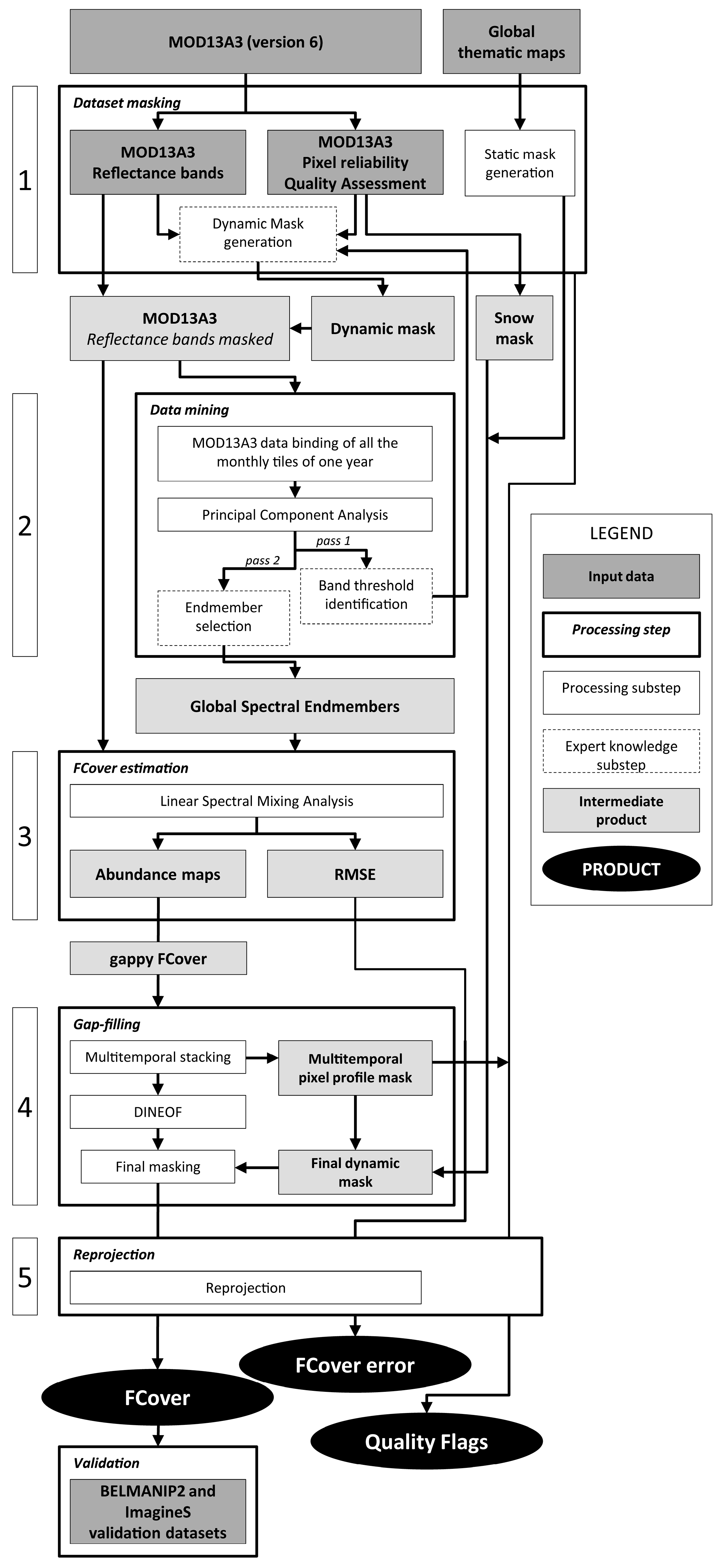
2.2. FCover Processing Chain

The MODIS-derived monthly gap-filled FCover product is the result of a processing chain specifically developed to cope with the expressed needs of users and science communities [18], data quality issues (original data quality flag), and thematic accuracy issues (ocean and coastal waters, non-vegetated arid deserts, ice, and large urban areas are excluded from processing). MOD13A3 collection 6 was used to generate the global FCover variable through 5 processing steps (Figure 1): (1) dataset masking; (2) data mining; (3) FCover estimation; (4) gap-filling; (5) reprojection and finally direct and indirect validations were performed on the generated FCover product.

All analyses were performed in R [37] using the packages raster [38], RSpectra [39], sinkr [40] and rtsa (under development by this paper authors, available at: https://github.com/ec-ecopotential/rtsa); SNAP [41]; and python with the support of GDAL library [42].

2.2.1. Dataset Masking

The dataset masking allows for the adoption of a pixel mask to exclude pixels from further processing by combining a static pixel mask with a dynamic pixel mask. The static pixel mask was created for each of the 271 MODIS tiles to remove pixels corresponding to oceans, water bodies, non-vegetated arid deserts, permanent snow and large urban areas. The data used to build the static mask (Table S1) are global products generated by the European Space Agency (ESA), the Consultative Group for International Agricultural Research—Consortium for Spatial Information (CGIAR-CSI) and NASA and mostly refer to 2010.

The dynamic pixel mask was generated for each of the 52845 MOD13A3 monthly product tiles using the VI Quality detailed QA layer (Table S2), pixel reliability summary QA layer (Table S3), blue reflectance band threshold for conservative cloud removal [43], and extremely bright pixels and pixels exhibiting ‘no data’ in at least one of the reflectance bands of the source MODIS tile.

In addition, the snow pixel cover information retrieved from each MODIS VI Quality detailed QA layer was used to generate a dynamic snow mask applied after the gap-filling together with the static mask.

2.2.2. Data Mining

A three-endmember linear mixture model (substrate, vegetation, dark surface i.e., SVD model) was used to estimate the FCover through linear spectral mixture analysis (LSMA) [44]. The linear mixture model provides physical representations of land surface reflectance as continuous fields of spectral endmember abundances [44]. Inverting the linear mixture model yields quantitative estimates of the areal abundance (fractional cover) within each pixel of the land cover types identified by the selected endmembers [45].

To perform data mining to select the three global spectral endmembers, principal component analysis (PCA) was applied on a representative global composite dataset consisting of all the MOD13A3 monthly tiles (i.e., 3252) at a global scale acquired over one year. Year 2001 was selected as representative because it has been identified as a reference climatic year without significant trends [46] and, additionally, the MODIS sensor aboard Terra satellite was in its initial acquisition lifetime and thus less subject to degradation [36,47]. First, resulting principal components generated from the MODIS reflectance data were orthogonally combined in a scatterplot of pixels (called the mixing space) to identify global spectral endmembers (i.e., pure pixels) [44,48,49] at the apexes of the mixing space, while the mixed pixels, namely, the pixels with spectral mixtures of different cover typologies, are located between the apexes.

2.2.3. FCover Estimation

LSMA has the ability to provide continuous fraction maps of endmember cover type abundance by analyzing the spectral mixture of reflectance within each pixel [50,51,52,53].

The assumption of the three-component mixture model is that the overall reflectance of a spectrally heterogeneous surface can be described as a linear combination of each spectral endmember reflectance [44]:

R (λ) = f_SE_S(λ) + f_VE_V(λ) + f_DE_D(λ),

(1)

where R(λ) is the overall reflectance at wavelength λ; E(λ) are the spectral endmembers corresponding to substrate (S), vegetation (V) and dark (D) identified from the mixing space; and f represents the fractional cover estimates.

When applying a constraint to the linear combination, the sum of the endmember fractional cover is forced to be equal to 1:

f_S + f_V + f_D = 1.

(2)

Each endmember fraction estimation is related to a single pixel and is accompanied by a root mean square error (RMSE) layer generated by the LSMA, which supplies a quantitative assessment of the estimation procedure.

By definition, the endmembers (i.e., the spectrally purest pixels) are found at the apexes of the triangular shape mixing space defined by the first principal components.

Among the few pixels at the apexes, we selected as substrate and vegetation endmembers those with the highest reflectance: the assumption is that the spectral variability within each cover type is fully enclosed by the purest pixel (i.e., endmember).

With regard to the methods for selecting endmembers other approaches are available (Pixel Purity Index (PPI), Count-Based endmember selection (CoB), Endmember Average Root mean square error (EAR), Minimum Average Spectral angle (MASA)) and they are computationally complex.

LSMA was applied to each MODIS monthly tile using the identified global spectral endmembers to estimate the FCover variable by extracting the vegetation fractional abundance f_V derived from the linear combination.

2.2.4. Gap-Filling

To overcome temporal gaps, the FCover product was gap-filled through the use of the data interpolating empirical orthogonal functions (DINEOF) technique [34,54]. The DINEOF technique has already been compared to optimal interpolation, demonstrating that more accurate results are achieved with up to 30 times less computational time [55], and was therefore selected as the methodology to reconstruct the time series of FCover products by gap-filling missing values.

DINEOF is a method for reconstructing missing data in multitemporal series of geophysical datasets and is based on empirical orthogonal functions (EOFs). The information of a spatio-temporal dataset can be efficiently synthesized by EOFs, each described by a spatial mode (2-dimensional map, also called “mode”) with its associated temporal mode (1-dimensional time series, also called “expansion coefficient” time series). The combination of the dominant EOF amplitudes returns the value of the field at the missing data points.

DINEOF is a procedure that fills gaps by iteratively decomposing the data field via singular value decomposition until a best solution is found compared to a subset of reference values (non-gappy). This procedure is performed by progressively including more EOFs in the reconstruction of the “gappy” locations until the minimization of error converges.

The FCover values of those pixels having a number of available observations lower than 30% were used for the calculation of the EOFs, and afterwards, the entire temporal profile of those pixels was used to generate a multitemporal pixel profile mask. DINEOF was run to gap-fill all FCover observations and subsequently those reconstructed pixels, corresponding to the multitemporal pixel profile mask or to the snow mask, were removed. Quality flags associated with each FCover monthly tile were generated at the pixel level to give the user community useful ancillary qualitative information related to the product. Quality flags are provided as a QF bit-coded layer generated in the processing procedure and give qualitative information about the usability and usefulness of the product related to the estimation of FCover using the adopted methodology. Table S4 reports the detailed description of the QF layer.

2.2.5. Reprojection

The gap-filled FCover global product was finally reprojected in a regular latitude/longitude grid (Plate Carrée) with the WGS 1984 ellipsoid (EPSG:4326) and adopting a new tiling system from the original MODIS sinusoidal projection (Figure S3), which was adopted for the entire dataset processing as the last processing step to avoid uncertainty propagation. The final FCover product spans from 60°S to 70°N for a total of 148 tiles on land.

2.3. FCover Product Validation

FCover product direct validation was performed using two global land product validation datasets as ground data: the CEOS BELMANIP2 (BEnchmark Land Multisite ANalysis and Intercomparison of Products) [56] and the ImagineS [57] products. FCover validation datasets are computed from the LAI and other canopy structural variables, such as leaf inclination and clumping. The FCover ground data values are averaged over 3 × 3 km sites and were acquired according to the guidelines defined in compliance with the protocols proposed by the CEOS Land Product Validation Subgroup [58,59]. The validation datasets well represent different latitudes and biomes in addition to cropland variability and consist of 107 FCover samples measured at 59 different sites. Indirect validation was performed by comparing the direct validation statistics calculated for the present product (MODV1) with those of other global FCover products (CYCV31 and GEOV1).

2.4. FCover Global Multitemporal Analysis

Basic statistical analysis (i.e., average and trend slope) was performed on the global gap-filled FCover product to provide a spatial representation of FCover average and the overall trend. The global FCover average was calculated as the average of all monthly values. The trend was calculated as the slope factor of a linear analysis computed for each pixel temporal profile using the generalized least squares (GLS) technique and represents the annual rate of increase or decrease in FCover. Considering that MODIS Terra data were available from February 2000, to have valid statistics for entire solar years, all of these analyses were calculated for the period 2001–2015.

In addition, at the application sites, the breaks for additive seasonal and trend (BFAST) technique [60] was applied to generate trend analysis and detect breaks in trends that could be the responses of vegetation to phenomena such as deforestation, fires, and urbanization. The BFAST technique allows for the decomposition of a time series into trends and seasonal and residual components to detect multiple abrupt changes and characterize their occurrence time, magnitude, and direction.

Temporal analysis was performed for the entire FCover product temporal span (2000–2015) by applying BFAST to single pixels selected for illustration.

3. Results

The newly generated MODV1 product (MOD Version 1) represents a consistent gap-filled FCover global product at a 1 km spatial resolution at a monthly timescale temporal granularity for the period 2000–2016 and is freely available upon request to the user community.

The FCover product is made available (upon request) in the NetCDF raster format with metadata according to the Climate and Forecast (CF) conventions v1.6. The product includes the following layers: FCover (gap-filled FCover estimation); FCover_error (RMSE error derived from LSMA procedure); and QF (Quality Flags associated with the FCover product).

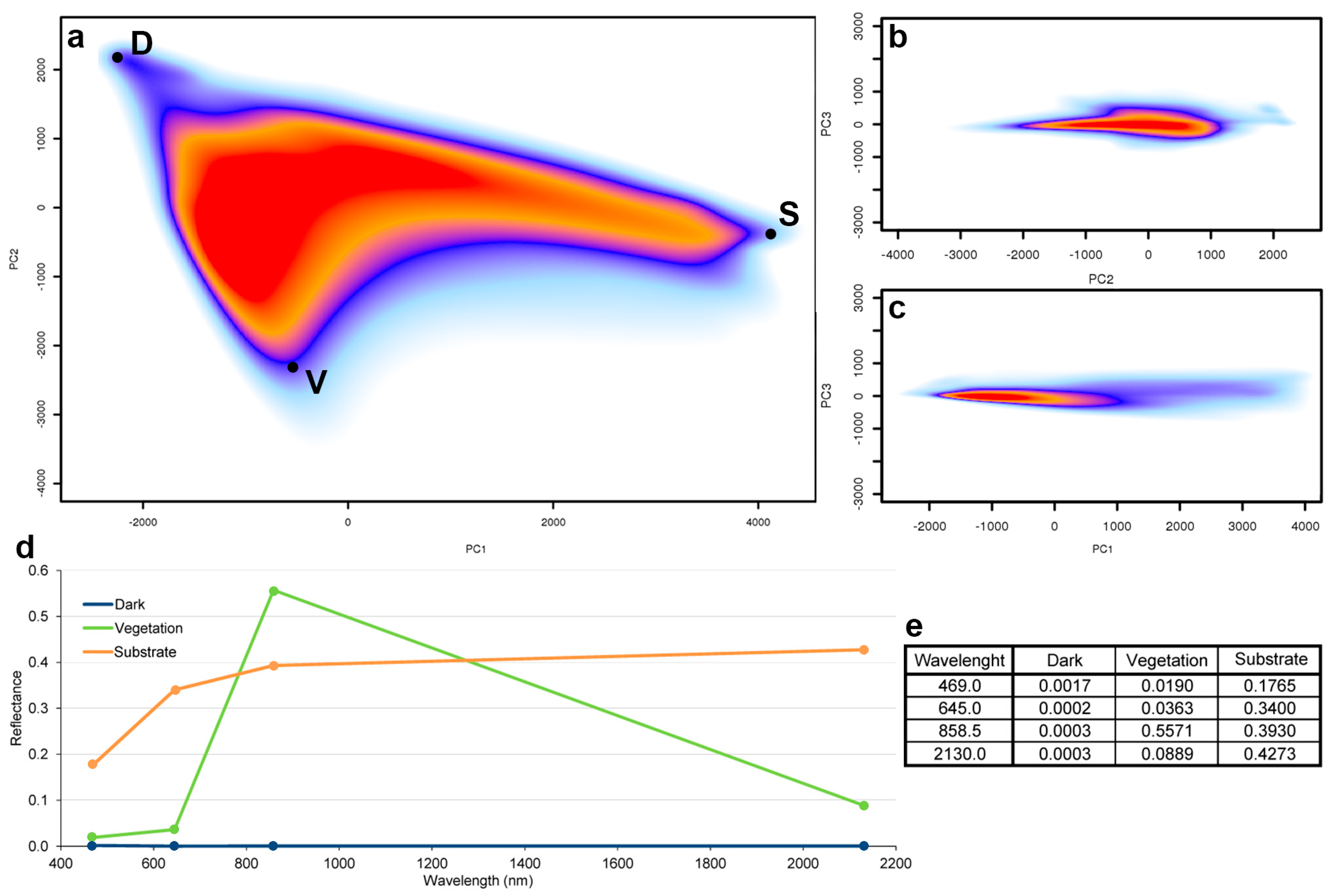
3.1. Linear Spectral Mixture Reflectance Models with Global Endmembers

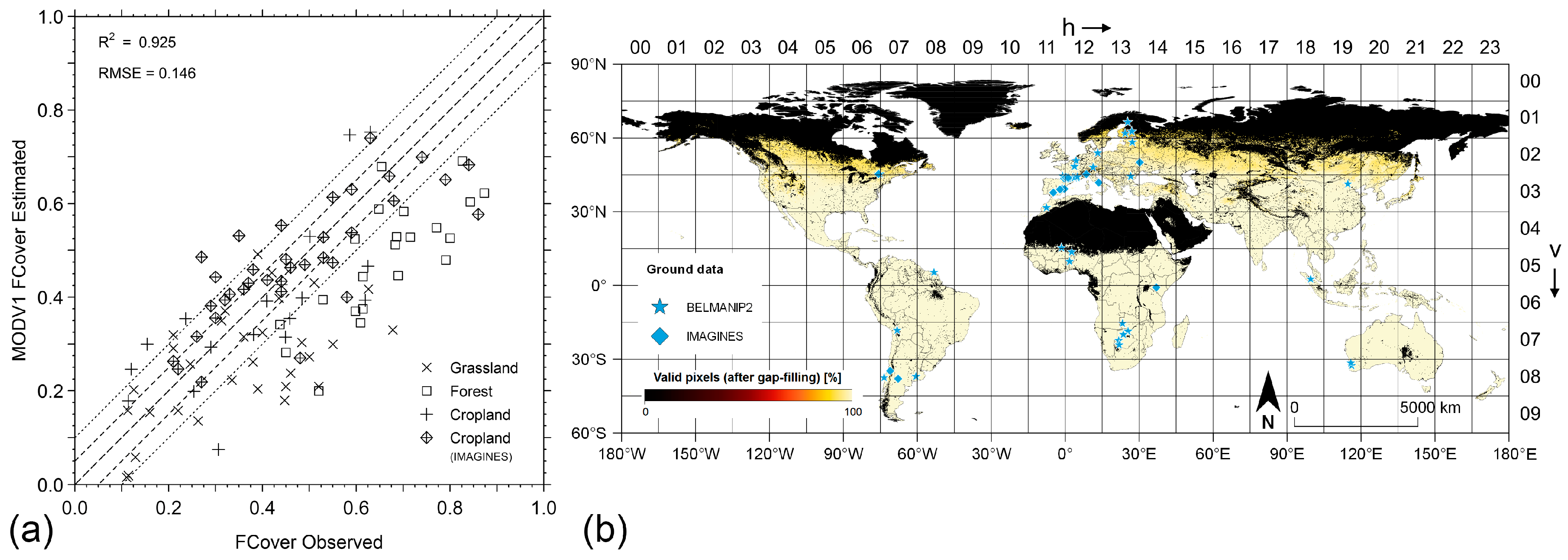
Using the LSMA technique from the global composite spectral mixing space (Figure 2a–c), three endmembers (endmembers = pure pixels) corresponding to substrate (S), vegetation (V), and dark surface (D) were identified (Figure 2d).

As expected, the geometry of the mixing space shown in Figure 2 as well as the spectra of the resulting V endmember are similar to those found by previous studies [44,48], with a peak reflectance value of 0.6 for V endmember and a minimum of 0.00 for D endmember. While dark and bright are distributed in the mixing space at the extremes of the first principal component, the V endmember is along the second principal component and occupies the third apex, generating the typical triangular plane of spectral mixtures. The S endmember corresponds to bright surfaces and is mostly associated with substrates except for extremely bright surfaces, in contrast to the D endmember, where the shadowing and residual water cover (after masking) are represented. The S endmember is substantially brighter across all wavelengths, but it is darker than the brightness observed in other studies, where the reflectance intensity ranges are larger due to the absence of dynamic and static masking processes.

The average and the standard deviation RMSE maps derived from FCover estimation with LSMA are shown in Figures S1 and S2 (Supplementary Materials).

3.2. Validation

Direct validation of the MODV1 product was performed considering all 107 samples available from the validation datasets. The results of the direct FCover product validation are reported in the scatterplot in Figure 3a. The MODV1 FCover estimated values are compared with the corresponding ground data, namely, the FCover observed values from validation datasets. Grassland in the Figure 3a legend refers to herbaceous, woody savanna and open shrubland; forest refers to broadleaf evergreen, broadleaf deciduous and mixed forests; and cropland refers to cultivated land. The ground data samples, as shown by their distribution in Figure 3b, account for different latitudes and biomes. The same figure also shows the percentage of valid monthly composite pixels after gap-filling and the new tiling system adopted for the WGS84 MODV1 projection.

The indirect validation results are shown in

Table 1. Comparison of statistics generated from the direct FCover MODV1 product validation with those generated from the other global FCover products: S_RES (dataset spatial resolution), T_RES (dataset temporal resolution), N (Number of samples), RMSE (Root Mean Square Error), B (average of the difference between the estimated FCover and the ground data), S (standard deviation of the difference between the estimated FCover and the ground data), R (correlation coefficient), R² (coefficient of determination), Slope (regression line slope), and Offset (regression line offset).

Product	Sensor	S_RES	T_RES	N	RMSE	B	S	R	R2	Slope	Offset	Reference
MODV1	MODIS/TERRA	1 km	1 month	107	0.146	0.065	0.132	0.741	0.925	0.88	0.11	Present study
GEOV1	PROBA-V	1 km	10 days	25	0.14	0.088	0.11	0.88	-	1.13	0.02	Sánchez et al., 2015
GEOV1	VGT/SPOT	1 km	10 days	65	0.095	0.019	0.093	-	0.848	0.98	0.02	Camacho et al., 2013
CYCV31	VGT/SPOT	1 km	10 days	60	0.177	−0.121	0.129	-	0.661	0.59	0.05	Camacho et al., 2013

, which reports all the compared products, their characteristics, the number of considered samples and the statistics related to the validation performances.

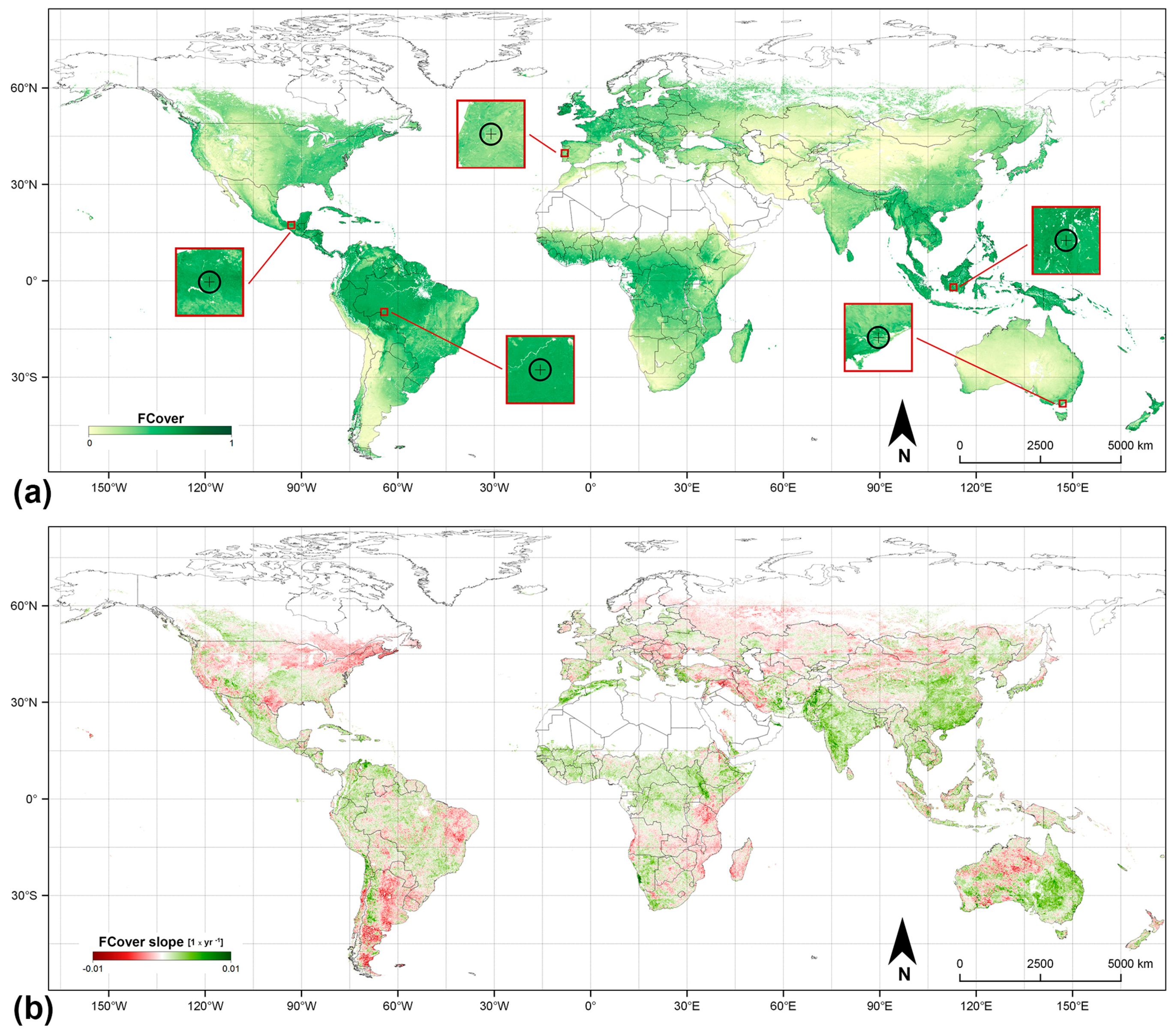
3.3. FCover Global Multitemporal Analysis Results

The basic statistics generated for the MODV1 global FCover time series are reported in Figure 4a, which shows the average FCover product, and Figure 4b, which shows the FCover temporal trend slope reported as annual rate.

The global FCover average computed for the period 2001–2015 ranges from 0 to 0.8. The white areas in Figure 4a correspond to masked pixels because they are permanently covered by water, desert, ice, snow, or anthropic cover, because the number of available observations is lower than 30% or because they are not considered reliable according to the QF layer.

As expected, the highest values (between 0.45 and 0.8) are concentrated close to the equator, where tropical rainforest is widespread and there is no dry season (tropical climate). This biome plays a key role in global carbon and energy cycles and is the most biodiverse terrestrial habitat, hosting approximately 50% of the world species [61]. High values are also shown in areas with temperate oceanic climates (according to the Koppen climate classification) such as Ireland, Great Britain and Northern France.

The temporal trend slope of the FCover global product, calculated as annual rate of increase or decrease of FCover for the period 2001–2015, ranges between −0.01 and 0.01.

All five continents show a mixed trend (i.e., both increasing and decreasing). Decreasing hotspots (values of approximately −0.005) can be noticed, for example, in North America (in the United States below the Great Lakes region), South America (Patagonia) and Asia (Al-Jazira province between the Syrian and Iraqi borders). Increasing FCover trend hotspots (values of approximately 0.004) are instead localized, for example, in Oceania (the eastern part of Australia), the Indian subcontinent (Pakistan and the western part of India), Africa (within the borders of Kenya, Uganda and South Sudan) and South America (around the Gulf of Venezuela).

4. Discussion

The resulting average FCover global distribution map is spatially consistent with the global representation of the vegetation spectral indexes, indicating that the LSMA method is valuable for deriving vegetation information using a spectral mixture model at the global scale [48,49]. This approach represents an effective and realistic method for FCover estimation and an alternative to the already existing algorithms that provide quite efficient estimations employing calibrated neural networks for the inversion of radiative transfer models and likely better account for leaf clumping [7]. The use of multiple endmembers is advised for land cover classification purposes [51] but at a global scale may generate biases in the FCover estimates between the different vegetation.

Therefore, addressing the global scale, the use of the SVD model (three-endmember linear mixture model) represents the correct simplification for generating consistent fractional abundances as demonstrated by works using LSMA [44,48] and adopting a small number of endmembers (three to four).

The three-endmember linear mixture model has already been demonstrated to be valid for the generation of a global linear mixture model from broadband multispectral imagery and is able to represent more than 95% of 30 million globally distributed LANDSAT ETM+ image spectra [44], to be highly correlated (correlation value of 0.95) with the greenness index estimated using Kauth-Thomas tasseled cap transformation [62], and to achieve the best performance for the estimation of FCover when compared to other methods such as multiple linear regression and Bayesian model averaging [63]. LSMA has been demonstrated to produce accurate results for the estimation of global vegetation fraction and exhibits a substantial linear relationship with EVI over a wide range of soils and a relative linear relationship with SAVI for most pixels with f_V > 0.2, although a substantial bias is present, and the variance is wide at low values [49].

DINOEF was selected as the gap-filling method considering the already known computational requirements, reliability of the reconstructed missing data, and ability to take advantage of both spatial and temporal information. Although the DINEOF algorithm has been discouraged for reconstructing missing values for terrestrial variables, due to its considerable memory requirements, the performance of such an algorithm for gap-filling missing FCover values was above expectations and had a reasonable computational cost effectiveness. Issues related to the selection of the gap-filling methodology, the detailed analysis of gap-filling performances [55] and the comparison of different gap-filling procedures are beyond the scope of this work.

The proposed methodological approach has a multiscale capability and can be easily adapted to work with different RS datasets and resolutions. For current and next-generation satellite data (e.g., the Sentinel satellites) with higher spatial and spectral resolutions, further development of the proposed approach may consider the use of multiple endmember spectral mixture analysis (MESMA) [64,65] regardless of whether more reflectance bands are available for fraction estimation and the adoption of the hierarchical empirical orthogonal function (HEOF) approach [66] as a gap-filling algorithm to address issues related to the computationally demanding processing of high-spatial resolution datasets. The HEOF algorithm has already been demonstrated to improve the accuracy and integrality of LAI products when applied to MODIS and CYCLOPES products [66].

Spatially and temporally explicit direct validation were performed using quantitative ground data FCover assessments collected from two different globally distributed datasets to evaluate product accuracy. The MODV1 FCover estimates show good agreement with the limited available ground data (Table 1), even though they generally tend to underestimate the ground references. With respect to the various biomes, the product estimates FCover well over croplands but generally underestimates FCover over forests. The good agreement between the FCover estimates and the ground data confirms that the global LSMA model is suitable for vegetation fractional cover estimates from broadband multispectral imagery, as was already stated by [44]. The MODV1 FCover product satisfies the BioPar User requirements in terms of thematic accuracy [18], fulfilling an absolute accuracy target threshold of 0.15.

Comparing the MODV1 direct validation result statistics to those derived from CYCV31 and GEOV1 [25,26], the accuracy of the MODV1 product appears consistent regardless of the considered criterion (Table 1) and even if different methodologies were adopted to estimate FCover from RS reflectances. Larger discrepancies in the FCover values observed over forest biomes have also been reported for GEOV1 as well as a positive offset [26] and some dispersion for intermediate values [25]. The MODV1 product tends to slightly underestimate the FCover ground data, in contrast to the overestimation found for GEOV1, even though this product is less relevant than the CYCV31 and is more associated with forest biomes, as revealed by the validation results (Table 1). The underestimation of FCover in forest biomes may be related to the higher light absorption of trees, which could increase the f_D value and decrease the f_V value. This evidence suggests that a biome-specific calibration of the algorithm, which is already adopted for the MODIS-derived LAI and FAPAR products [7], should be considered for future improvements in the global FCover estimation in future versions of the product.

The quality of the input MODIS product may have limited the FCover estimation accuracy. In fact, the algorithms for estimating the biophysical variables from MODIS reflectances have already been shown to have difficulty in describing very low LAI and FAPAR values [20], and the instability of MODIS reflectances in monthly composites may result in variable temporal profiles [67]. In addition, the stripe noise affecting MODIS reflectances [68], in particular the SWIR wavelengths, may introduce stripe artifacts in MODIS-derived products if an appropriate procedure using a stripe noise detection and removal algorithm is not performed by the MODIS Adaptive Processing System (MODAPS).

From the spatial distribution of the global FCover MODV1 average, it can be observed that a clear zonation emerges, and this zonation seems to be mostly influenced by the latitudinal gradient and the climatic zone classification. The highest values are found in areas where tropical rainforest occurs because this forest type maintains its greenness throughout the year. The FCover slope product, representing the annual rate of change, shows at a glance if the vegetation cover fraction trend over the examined period is increasing, decreasing or stable. In contrast to the average product, no clear global tendencies can be distinguished compared to previous findings from the NDVI dataset [69], but spatial patterns of increasing or decreasing vegetation can be identified.

Further analysis based on MODV1 product may reveal changes in the average values and trends when two or more different time spans are considered for time series analysis. MODV1, which provides information in space and over time on photosynthetically green vegetation presence and distribution and enables the quantification of gross loss and gain, could be useful in supporting the understanding of vegetation reaction/response to several natural and manmade phenomena and the evaluation of the effectiveness of adopted planning and management strategies.

As a general remark, information derived from this type of temporal analysis and coupled with the appropriate ecological modeling could be used as a proxy to assess biodiversity distributions and carbon storage capacity in a very rough manner while taking into account the FCover variation within the year. As a consequence, green vegetation cover information such as FCover could support the assessment of several ecosystem services (i.e., land use provisioning and regulation).

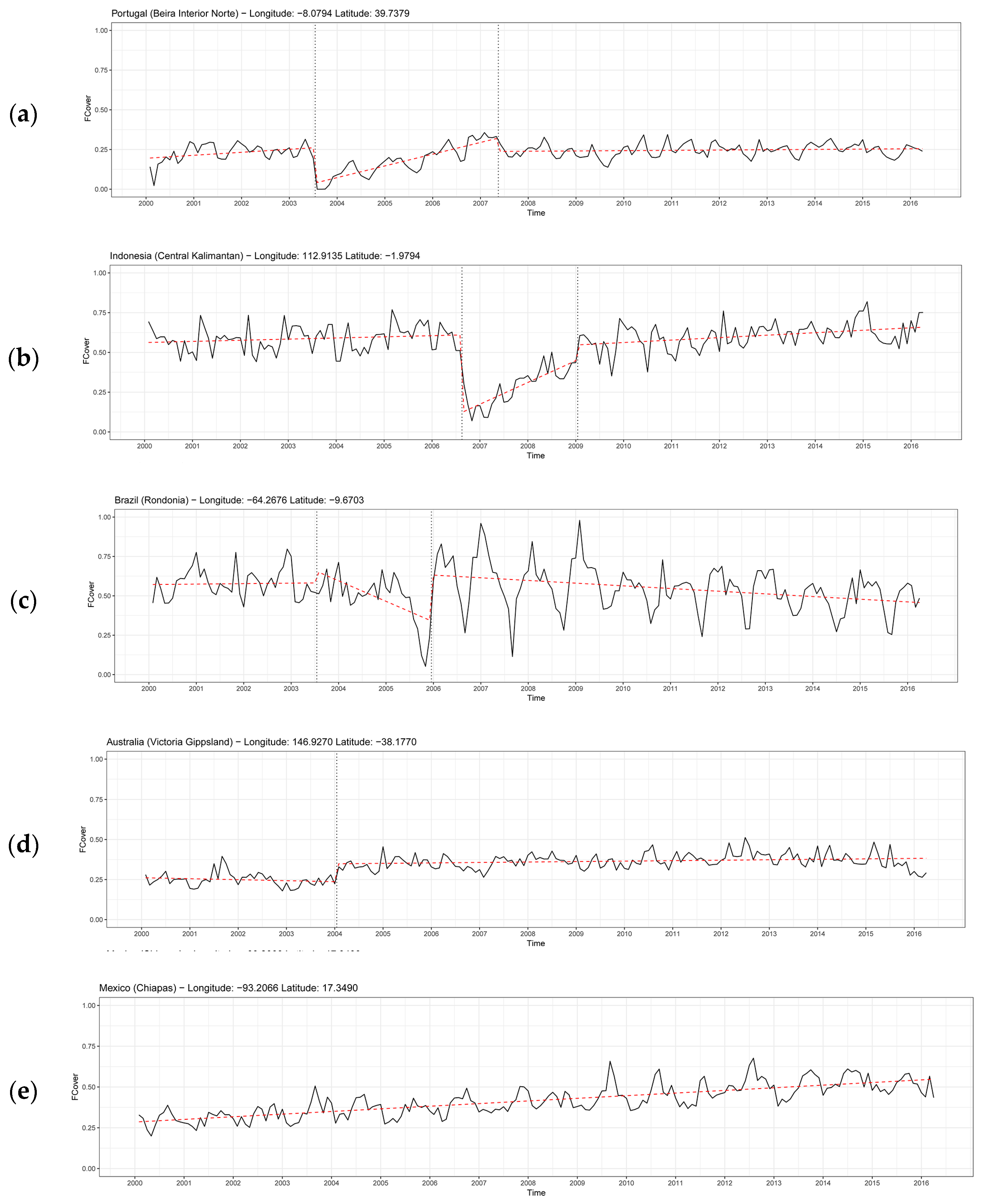
5. Application Sites

The multitemporal analysis of MODV1 could enable the identification of vegetation changes and provide a preliminary quantification of loss and gain, offering support to the interpretation of cause-effect relations of specific dynamics such as deforestation, fire severity, post-hazard vegetation restoration, land use change, and urbanization.

Application sites are presented in this section to demonstrate FCover MODV1 product suitability for monitoring vegetation responses to natural and manmade phenomena. Such processes can occur, alone or combined, at several temporal and spatial scales. With regard to temporal dimension, analysis can be carried out using the FCover product with two different approaches:

—

a priori, without any precise information on local processes, to detect areas where there has been a heavy change in vegetation cover (i.e., identification of break in temporal) and then, adding site-specific knowledge a/o information from other sources, to identify the phenomenon that occurred;

—

a posteriori, having already information on a certain process or phenomenon taking place in selected location, to find its confirmation through the dataset and monitor how it evolves in time.

The application sites here follow the a posteriori approach, namely, previous knowledge of the causes of vegetation changes (slow or abrupt) was collected from the literature. Such knowledge was then associated with multitemporal analysis results to confirm the underlying processes and events and observe how they affect FCover values over time.

Five application sites, represented by single pixels, were selected to analyze the vegetation cover changes that occurred at the local scale, were chosen according to different cause-effect phenomena (e.g., wildfires and deforestation), in different biomes (e.g., tropical rainforests, subtropical dry forests, and Mediterranean vegetation) and are specifically located in Portugal, Indonesia, Brazil, Australia, and Mexico. For all the application sites, trend analysis and break detection were performed, and the results are reported in Figure 5, which shows the FCover temporal profiles with the corresponding trends estimated between the detected breaks.

The FCover values over time are constant in Beira Baixa (Portugal) and for the most part range from 0.13 to 0.35. From 2000 to the first half of 2003, the trend is slightly increasing. A single relevant event can be observed in the second half of 2003 that brought FCover down from approximately 0.25 to 0 in a very short time, and then, it remains at 0 for a few months. Then, FCover began to increase again until the second half of 2007, when having reached values comparable to those prior to 2003, it slowed down and remained constant. The sharp and sudden decline in FCover values in 2003 matches the information on wildfires that occurred in May/June of that year [70]. After a few months, during which vegetation was completely absent, FCover began to increase slowly but continuously in accordance with the regeneration process time frame [71]. As indicated by the chart, in approximately three years, the cover values return to those observed prior to the event (approximately 0.25).

The central Kalimantan (Indonesia) FCover temporal profile shows an almost constant trend (values oscillating between 0.45 and 0.75) except for during the period between the second half of year 2006 and the beginning of year 2009. The Indonesian case is emblematic because it shows the effect of a phenomenon that is widespread in the country [72], namely, the replacement of tropical rainforest with oil palm tree plantations. This phenomenon threatens biodiversity [72], is a source of carbon emissions [73] and has a high social-cultural impact (both positive and negative). The temporal profile perfectly represents the evolution of this phenomenon, and in fact, the values up until 2006 correspond to undisturbed tropical rainforest, while the drop-in values, lasting for some months, corresponds to deforestation activities. Later, a rapid increase in FCover percentage (i.e., very positive trend slope) reflects the fact that palm oil plants grow quite fast, and finally, a vegetation fraction similar to or higher than the initial one is found. There was no change in the cover between initial and final conditions, but from ecological, biodiversity, economic, and social-cultural points of view, the change was impressive.

In Rondonia (Brazil), the FCover for the period 2000–2016 exhibited four distinct behaviors in the temporal profile. The first was from 2000 to the first half of 2003 (values oscillating between 0.4 and 0.8), the second was from the second half of 2003 to 2006 (a strong break can be noticed), the third was from 2006 to the first months of 2009 (values oscillating between 0.25 and 0.96), and the fourth was from 2009 onwards (values oscillating between 0.25 and 0.7). After 2006, FCover showed higher fluctuations than in the past period that decreased over time. The FCover trend at the beginning of the considered period is slightly increasing and then strongly decreases, and after 2006, the FCover keeps on decreasing at a low annual rate. Deforestation is a widespread phenomenon in Rondonia, where it started in the mid-1970s. Among the driving factors are logging, agriculture, mining, and cattle ranching [74]. Observing the Brazilian pixel temporal profile between 2003 and 2006, the FCover values decrease slowly at the beginning, and this could be attributed to logging activities, while at a certain point, this process seems to have an acceleration (end of 2005) that brings the cover percentage to less than 0.1 (from a value of approximately 0.5). This very rapid change in vegetation extent corresponds to a well-known strategy of clearing forest areas to be replaced with pastures for cattle [75]. After 2006, the FCover values suggest that other vegetation types, in this case, a mixture of cropland and pastures, replaced the tropical rainforest. Nevertheless, after a few years, starting in 2010, the highest values slowly decrease, likely due to soil fertility depletion.

The Gippsland location (Australia) shows a slightly decreasing trend until 2004. From 2004 onwards, the values start increasing slowly but continuously, and at the end of the examined period, FCover reaches 0.50 (increasing on average of 0.1). In particular, the trend analysis indicates a break in 2004 that signifies the trend change. The FCover value fluctuations remain almost the same over time. By analyzing archival EO images for the Australian site, it seems that the considered location underwent a change in cover from agriculture to forest plantation. The slightly decreasing trend in the first period of the profile, when the pixel was covered by crops, associated with somewhat irrelevant fluctuations, could not be interpreted without additional site-specific information (e.g., climatic conditions and crop health).

The selected Mexican site is in the active area of the El Chichon volcano in northwest Chiapas. The FCover values in 2000 are approximately 0.3 on average, and their fluctuations vary among years, and then, a value of approximately 0.5 on average is reached in 2016. The Mexican site presents an example of a gradual, slow and almost continuous FCover growing trend. This area, which is now mainly covered by shrubs, is in a location very close to the volcano crater (~2.5 km); therefore, eruptions that occurred in the past (i.e., in 1982) exposed it to pyroclastic surges and thick tephra fallout. As an active volcanic area, the long-term trend increase of vegetation cover fraction could be interpreted as the long-term process of vegetation recovery [76].

MODV1 multitemporal analysis enabled the identification and preliminary quantification of several phenomena and processes related to vegetation cover and distribution, such as deforestation, fires, and natural hazards. This kind of analysis, applied in this study to single pixels, profits from the extended temporal product extent and could help gain information on vegetation dynamics. These results demonstrate that knowledge derived from MODV1 FCover products is relevant to supporting the assessment of issues related to soil, biodiversity, ecosystem services and other environmental components and dynamics related to vegetation presence, absence, permanence, distribution, and cover.

Vegetation indeed influences land-atmosphere exchanges of carbon, water and energy, and green vegetation fraction cover is used to partition the vegetation contributions in these exchanges in land surface models for weather forecasting, hydrology, regional and global climate studies, and global change monitoring.

6. Conclusions

This paper presents the new global MODV1 FCover product that is freely available to the user community upon request to the corresponding author. It has been generated from over 15 years of MODIS monthly observations and extends the already available collections of satellite-derived FCover products. The novel technical approaches of this product include the use of the linear spectral mixture technique to estimate global FCover and the adoption of the data interpolating empirical orthogonal functions algorithm to take advantage of all non-missing available pixels in both the spatial and temporal dimensions to gap-fill missing satellite observations. The developed processing chain could be easily adapted to other satellite remote sensing datasets, such as the Sentinel datasets. The generated MODV1 FCover product was validated with two global land validation datasets and showed an overall good thematic absolute accuracy that is consistent with the validation performances of existing FCover global products. The product information and detection capability have been shown by means of basic statistics at the global scale and through local multitemporal analysis of selected sites, describing different dynamics resulting from cause-effect phenomena. Considering the results obtained from the analysis, from a wider perspective, the potential of MODV1 as a gap-filled product could be even better exploited by assimilating the product into existing environmental models that address ecosystem processes, functions and services.

References

1. Pereira, H.; Ferrier, S.; Walters, M.; Geller, N.; Jongman, R.H.G.; Scholes, J.; Bruford, M.; Brummitt, N.; Butchart, S.; Cardoso, A.; et al. Essential Biodiversity Variables. Science 2013, 339, 277–278. [Google Scholar] [CrossRef] [PubMed] [Green Version]
2. Guerra, C.; Pinto-Correia, T.; Metzger, M.J. Mapping Soil Erosion Prevention Using an Ecosystem Service Modeling Framework for Integrated Land Management and Policy. Ecosystems 2014, 17, 878–889. [Google Scholar] [CrossRef]
3. Bennett, E.M.; Cramer, W.; Begossi, A.; Cundill, G.; Díaz, S.; Egoh, B.N.; Geijzendorffer, I.R.; Krug, C.B.; Lavorel, S.; Lazos, E.; et al. Linking biodiversity, ecosystem services, and human well-being: Three challenges for designing research for sustainability. Curr. Opin. Environ. Sustain. 2015, 14, 76–85. [Google Scholar] [CrossRef]
4. De Sousa, C.A. Turning brownfields into green space in the City of Toronto. Landsc. Urban Plan. 2003, 62, 181–198. [Google Scholar] [CrossRef]
5. Sanesi, G.; Colangelo, G.; Lafortezza, R.; Calvo, E.; Davies, C. Urban green infrastructure and urban forests: A case study of the Metropolitan Area of Milan. Landsc. Res. 2017, 42, 164–175. [Google Scholar] [CrossRef]
6. Herrmann, S.M.; Anyamba, A.; Tucker, C.J. Recent trends in vegetation dynamics in the African Sahel and their relationship to climate. Glob. Environ. Chang. 2005, 15, 394–404. [Google Scholar] [CrossRef]
7. Bacour, C.; Baret, F.; Béal, D.; Weiss, M.; Pavageau, K. Neural network estimation of LAI, fAPAR, fCover and LAI× C ab, from top of canopy MERIS reflectance data: Principles and validation. Remote Sens. Environ. 2006, 105, 313–325. [Google Scholar] [CrossRef]
8. Fu, B.; Liu, Y.; Lü, Y.; He, C.; Zeng, Y.; Wu, B. Assessing the soil erosion control service of ecosystems change in the Loess Plateau of China. Ecol. Complex. 2011, 8, 284–293. [Google Scholar] [CrossRef]
9. Guerra, C.; Maes, J.; Geijzendorffer, I.; Metzger, M.J. An assessment of soil erosion prevention by vegetation in Mediterranean Europe: Current trends of ecosystem service provision. Ecol. Indic. 2016, 60, 213–222. [Google Scholar] [CrossRef]
10. Turner, W.; Spector, S.; Gardiner, N.; Fladeland, M.; Sterling, E.; Steininger, M. Remote sensing for biodiversity science and conservation. Trends Ecol. Evol. 2003, 18, 306–314. [Google Scholar] [CrossRef]
11. Clerici, N.; Weissteiner, C.J.; Gerard, F. Exploring the use of MODIS NDVI-based phenology indicators for classifying forest general habitat categories. Remote Sens. 2012, 4, 1781–1803. [Google Scholar] [CrossRef] [Green Version]
12. Wan, Z.; Wang, P.; Li, X. Using MODIS land surface temperature and normalized difference vegetation index products for monitoring drought in the southern Great Plains, USA. Int. J. Remote Sens. 2004, 25, 61–72. [Google Scholar] [CrossRef]
13. Kim, K.; Wang, M.C.; Ranjitkar, S.; Liu, S.H.; Xu, J.C.; Zomer, R.J. Using leaf area index (LAI) to assess vegetation response to drought in Yunnan province of China. J. Mt. Sci. 2017, 14, 1863–1872. [Google Scholar] [CrossRef]
14. Tacker, C.J. Red and photographic infrared linear combination for monitoring vegetation. Remote Sens. Environ. 1979, 8, 127–150. [Google Scholar] [CrossRef]
15. Carlson, T.N.; Ripley, D.A. On the relation between NDVI, fractional vegetation cover, and leaf area index. Remote Sens. Environ. 1997, 62, 241–252. [Google Scholar] [CrossRef]
16. Myneni, R.B.; Williams, D.L. On the relationship between FAPAR and NDVI. Remote Sens. Environ. 1994, 49, 200–211. [Google Scholar] [CrossRef]
17. Navarro, L.; Fernández, N.; Guerra, C.; Pereira, H.M.; Turak, E.; Yahara, T.; Kissling, W.D.; Skidmore, A.; Kim, E.S.; Kim, H.; et al. Monitoring biodiversity change through effective global coordination. Curr. Opin. Environ. Sustain. 2017, 29, 158–169. [Google Scholar] [CrossRef]
18. Lacaze, R.; Atzberger, C.; Bartholomé, E.; Combal, B.; Calvet, J.C.; Lefèvre, V.; Olsson, B. BioPar User Requirements; GEOLAND: San Jose, CA, USA, 2009. [Google Scholar]
19. Chen, J.M.; Pavlic, G.; Brown, L.; Cihlar, J.; Leblanc, S.G.; White, H.P.; Hall, R.J.; Peddle, D.R.; King, D.J.; Trofymow, J.A.; et al. Derivation and validation of Canada-wide coarse-resolution leaf area index maps using high-resolution satellite imagery and ground measurements. Remote Sens. Environ. 2002, 80, 165–184. [Google Scholar] [CrossRef]
20. Weiss, M.; Baret, F.; Garrigues, S.; Lacaze, R. LAI and fAPAR CYCLOPES global products derived from VEGETATION. Part 2: Validation and comparison with MODIS collection 4 products. Remote Sens. Environ. 2007, 110, 317–331. [Google Scholar] [CrossRef]
21. Duveiller, G.; Lopez-Lozano, R.; Cescatti, A. Exploiting the multi-angularity of the MODIS temporal signal to identify spatially homogeneous vegetation cover: A demonstration for agricultural monitoring applications. Remote Sens. Environ. 2015, 166, 61–77. [Google Scholar] [CrossRef]
22. Baret, F.; Hagolle, O.; Geiger, B.; Bicheron, P.; Miras, B.; Huc, M.; Berthelot, B.; Niño, F.; Weiss, M.; Samain, O.; et al. LAI, fAPAR and fCover CYCLOPES global products derived from VEGETATION: Part 1: Principles of the algorithm. Remote Sens. Environ. 2007, 110, 275–286. [Google Scholar] [CrossRef] [Green Version]
23. Baret, F.; Weiss, M.; Lacaze, R.; Camacho, F.; Makhmara, H.; Pacholcyzk, P.; Smets, B. GEOV1: LAI and FAPAR essential climate variables and FCOVER global time series capitalizing over existing products. Part 1: Principles of development and production. Remote Sens. Environ. 2013, 137, 299–309. [Google Scholar] [CrossRef]
24. Camacho, F.; Cernicharo, J.; Lacaze, R.; Baret, F.; Weiss, M. GEOV1: LAI, FAPAR essential climate variables and FCOVER global time series capitalizing over existing products. Part 2: Validation and Intercomparison with reference products. Remote Sens. Environ. 2013, 137, 310–329. [Google Scholar] [CrossRef]
25. Sánchez, J.; Camacho, F.; Lacaze, R.; Smets, B. Early validation of PROBA-V GEOV1 LAI, FAPAR and FCOVER products for the continuity of the Copernicus Global Land Service. Int. Arch. Photogramm. Remote Sens. Spat. Inf. Sci. 2015, 40, 93. [Google Scholar] [CrossRef]
26. Myneni, R.B.; Knyazikhin, Y.; Park, T.; MOD15A2H MODIS/Terra Leaf Area Index/FPAR 8-Day L4 Global 500 m SIN Grid V006. NASA EOSDIS Land Processes DAAC. 2015. Available online: https://lpdaac. usgs. gov/dataset_discovery/modis/modis_products_table/mod15a2h_v006 (accessed on 14 December 2017).
27. Didan, K.; MOD13A3 MODIS/Terra Vegetation Indices Monthly L3 Global 1 km SIN Grid V006. NASA EOSDIS Land Processes DAAC. 2015. Available online: https://lpdaac.usgs.gov/dataset_discovery/modis/modis_products_table/mod13a3_v006 (accessed on 14 December 2017).
28. King, M.D.; Kaufman, Y.J.; Menzel, W.P.; Tanre, D. Remote sensing of cloud, aerosol, and water vapor properties from the Moderate Resolution Imaging Spectrometer (MODIS). IEEE Trans. Geosci. Remote Sens. 1992, 30, 2–27. [Google Scholar] [CrossRef]
29. Chen, J.; Jönsson, P.; Tamura, M.; Gu, Z.; Matsushita, B.; Eklundh, L. A simple method for reconstructing a high-quality NDVI time-series data set based on the Savitzky-Golay filter. Remote Sens. Environ. 2004, 91, 332–344. [Google Scholar] [CrossRef]
30. Tan, B.; Morisette, J.T.; Wolfe, R.E.; Gao, F.; Ederer, G.A.; Nightingale, J.; Pedelty, J.A. An enhanced TIMESAT algorithm for estimating vegetation phenology metrics from MODIS data. IEEE J. Sel. Top. Appl. Earth Obs. Remote Sens. 2011, 4, 361–371. [Google Scholar] [CrossRef]
31. Eilers, P.H.C. A perfect smoother. Anal. Chem. 2003, 75, 3631–3636. [Google Scholar] [CrossRef] [PubMed]
32. Atkinson, P.M.; Jeganathan, C.; Dash, J.; Atzberger, C. Inter-comparison of four models for smoothing satellite sensor time-series data to estimate vegetation phenology. Remote Sens. Environ. 2012, 123, 400–417. [Google Scholar] [CrossRef]
33. Neteler, M. Estimating daily land surface temperatures in mountainous environments by reconstructed MODIS LST data. Remote Sens. 2010, 2, 333–351. [Google Scholar] [CrossRef]
34. Beckers, J.M.; Rixen, M. EOF Calculations and Data Filling from Incomplete Oceanographic Datasets. J. Atmos. Ocean. Technol. 2003, 20, 1839–1856. [Google Scholar] [CrossRef]
35. Gerber, F.; Furrer, R.; Schaepman-Strub, G.; de Jong, R.; Schaepman, M.E. Predicting missing values in spatio-temporal satellite data. arXiv, 2016; arXiv:1605.01038. [Google Scholar]
36. Lyapustin, A.; Wang, Y.; Xiong, X.; Meister, G.; Platnick, S.; Levy, R.; Franz, B.; Korkin, S.; Hilker, T.; Tucker, J.; et al. Scientific impact of MODIS C5 calibration degradation and C6+ improvements. Atmos. Meas. Technol. 2014, 7, 4353–4365. [Google Scholar] [CrossRef]
37. Core Team. R: A language and environment for statistical computing. In R Foundation for Statistical Computing; Core Team: Vienna, Austria, 2016. [Google Scholar]
38. Hijmans, R.J. Raster: Geographic Data Analysis and Modeling. Available online: https://CRAN.R-project.org/package=raster (accessed on 14 December 2017).
39. Qiu, Y.; Mei, J. RSpectra: Solvers for Large Scale Eigenvalue and SVD Problems. Available online: https://CRAN.R-project.org/package=RSpectra (accessed on 14 December 2017).
40. Taylor, M. Sinkr: Collection of Functions with Emphasis in Multivariate Data Analysis. Available online: https://github.com/marchtaylor/sinkr (accessed on 14 December 2017).
41. SNAP Core Team SNAP: ESA Sentinel Application Platform v4.0. Available online: http://step.esa.int (accessed on 14 December 2017).
42. GDAL. Geospatial Data Abstraction Library, Open Source Geospatial Foundation. Available online: http://gdal.osgeo.org (accessed on 14 December 2017).
43. Manfron, G.; Crema, A.; Boschetti, M.; Confalonieri, R. Testing automatic procedures to map rice area and detect phenological crop information exploiting time series analysis of remote sensed MODIS data. In Proceedings of the SPIE 8531, Remote Sensing for Agriculture, Ecosystems, and Hydrology XIV, Edinburgh, UK, 24–26 September 2012. [Google Scholar]
44. Small, C. The Landsat ETM+ spectral mixing space. Remote Sens. Environ. 2004, 93, 1–17. [Google Scholar] [CrossRef]
45. Adams, J.B.; Smith, M.O.; Johnson, P.E. Spectral mixture modeling: A new analysis of rock and soil types at the viking lander 1 site. J. Geophys. Res. 1986, 91, 8089–8122. [Google Scholar] [CrossRef]
46. Zhang, K.; Kimball, J.S.; Nemani, R.R.; Running, S.W.; Hong, Y.; Gourley, J.J.; Yu, Z. Vegetation greening and climate change promote multidecadal rises of global land evapotranspiration. Sci. Rep. 2015, 5, 15956. [Google Scholar] [CrossRef] [PubMed]
47. Wang, D.; Morton, D.; Masek, J.; Wu, A.; Nagol, J.; Xiong, X.; Levy, R.; Vermote, E.; Wolfe, R. Impact of sensor degradation on the MODIS NDVI time series. Remote Sens. Environ. 2012, 119, 55–61. [Google Scholar] [CrossRef]
48. Small, C.; Milesi, C. Multi-scale standardized spectral mixture models. Remote Sens. Environ. 2013, 136, 442–454. [Google Scholar] [CrossRef]
49. Sousa, D.; Small, C. Global cross-calibration of Landsat spectral mixture models. Remote Sens. Environ. 2017, 192, 139–149. [Google Scholar] [CrossRef]
50. Taramelli, A.; Valentini, E.; Innocenti, C.; Cappucci, S. FHYL: Field spectral libraries, airborne hyperspectral images and topographic and bathymetric LiDAR data for complex coastal mapping. In Proceedings of the 2013 IEEE International Geoscience and Remote Sensing Symposium-IGARSS, Melbourne, Australia, 21–26 July 2013; pp. 2270–2273. [Google Scholar]
51. Valentini, E.; Taramelli, A.; Filipponi, F.; Giulio, S. An effective procedure for EUNIS and Natura 2000 habitat type mapping in estuarine ecosystems integrating ecological knowledge and remote sensing analysis. Ocean Coast. Manag. 2015, 108, 52–64. [Google Scholar] [CrossRef]
52. Manzo, C.; Valentini, E.; Taramelli, A.; Filipponi, F.; Disperati, L. Spectral characterization of coastal sediments using Field Spectral Libraries, Airborne Hyperspectral Images and Topographic LiDAR Data (FHyL). Int. J. Appl. Earth Obs. Geoinf. 2015, 36, 54–68. [Google Scholar] [CrossRef]
53. Taramelli, A.; Valentini, E.; Cornacchia, L.; Bozzeda, F. A hybrid power law approach for spatial and temporal pattern analysis of salt marsh evolution. J. Coast. Res. 2017, 77, 62–72. [Google Scholar] [CrossRef]
54. Taylor, M.H.; Losch, M.; Wenzel, M.; Schroeter, J. On the Sensitivity of Field Reconstruction and Prediction Using Empirical Orthogonal Functions Derived from Gappy Data. J. Clim. 2013, 26, 9194–9205. [Google Scholar] [CrossRef] [Green Version]
55. Alvera-Azcárate, A.; Barth, A.; Rixen, M.; Beckers, J.M. Reconstruction of incomplete oceanographic data sets using empirical orthogonal functions: Application to the Adriatic Sea surface temperature. Ocean Model. 2005, 9, 325–346. [Google Scholar] [CrossRef] [Green Version]
56. Baret, F.; Morissette, J.; Fernandes, R.; Champeaux, J.L.; Myneni, R.; Chen, J.; Plummer, S.; Weiss, M.; Bacour, C.; Garrigue, S.; et al. Evaluation of the representativeness of networks of sites for the global validation and intercomparison of land biophysical products. Proposition of the CEOS-BELMANIP. IEEE Trans. Geosci. Remote Sens. 2006, 44, 1794–1803. [Google Scholar] [CrossRef]
57. Camacho, F.; Lacaze, R.; Latorre, C.; Baret, F.; De la Cruz, F.; Demarez, V.; Di Bella, C.; García-Haro, J.; Pat González-Dugo, M.; Kussul, N.; et al. Collection of Ground Biophysical Measurements in support of Copernicus Global Land Product Validation: The ImagineS database. Geophys. Res. Abstr. 2015, 17, EGU2015-2209-1. [Google Scholar]
58. Fernandes, R.; Plummer, S.; Nightingale, J.; Baret, F.; Camacho, F.; Fang, H.; LeBlanc, S. Global Leaf Area Index Product Validation Good Practices. In Best Practice for Satellite-Derived Land Product Validation; Schaepman-Strub, G., Román, M., Nickeson, J., Eds.; Land Product Validation Subgroup (WGCV/CEOS): Greenbelt, MD, USA, 2014. [Google Scholar]
59. Morisette, J.T.; Baret, F.; Privette, J.L.; Myneni, R.B.; Nickeson, J.E.; Garrigues, S.; Shabanov, N.V.; Weiss, M.; Fern, R.A.; Leblanc, S.G.; et al. Validation of global moderate-resolution LAI products: A framework proposed within the CEOS land product validation subgroup. IEEE Trans. Geosci. Remote Sens. 2006, 44, 1804. [Google Scholar] [CrossRef]
60. Verbesselt, J.; Hyndman, R.; Newnham, G.; Culvenor, D. Detecting Trend and Seasonal Changes in Satellite Image Time Series. Remote Sens. Environ. 2010, 114, 106–115. [Google Scholar] [CrossRef]
61. Wright, S.J. Tropical forests in a changing environment. Trends Ecol. Evol. 2005, 20, 553–560. [Google Scholar] [CrossRef] [PubMed]
62. Kauth, R.J.; Thomas, G.S. The tasselled cap—A graphic description of the spectral-temporal development of agricultural crops as seen by Landsat. Lab. Appl. Remote Sens. Symp. 1976, 1, 159. [Google Scholar]
63. Jia, K.; Li, Y.; Liang, S.; Wei, X.; Yao, Y. Combining Estimation of Green Vegetation Fraction in an Arid Region from Landsat 7 ETM+ Data. Remote Sens. 2017, 9, 1121. [Google Scholar] [CrossRef]
64. Roberts, D.A.; Gardner, M.; Church, R.; Ustin, S.; Scheer, G.; Green, R.O. Mapping chaparral in the Santa Monica Mountains using multiple endmember spectral mixture models. Remote Sens. Environ. 1998, 65, 267–279. [Google Scholar] [CrossRef]
65. Degerickx, J.; Okujeni, A.; Iordache, M.D.; Hermy, M.; van der Linden, S.; Somers, B. A Novel Spectral Library Pruning Technique for Spectral Unmixing of Urban Land Cover. Remote Sens. 2017, 9, 565. [Google Scholar] [CrossRef]
66. Wang, D.; Liang, S. Integrating MODIS and CYCLOPES leaf area index products using empirical orthogonal functions. IEEE Trans. Geosci. Remote Sens. 2011, 49, 1513–1519. [Google Scholar] [CrossRef]
67. Verger, A.; Baret, F.; Weiss, M. Performances of neural networks for deriving LAI estimates from existing CYCLOPES and MODIS products. Remote Sens. Environ. 2008, 112, 2789–2803. [Google Scholar] [CrossRef]
68. Rakwatin, P.; Takeuchi, W.; Yasuoka, Y. Stripe noise reduction in MODIS data by combining histogram matching with facet filter. IEEE Trans. Geosci. Remote Sens. 2007, 45, 1844–1856. [Google Scholar] [CrossRef]
69. Liu, Y.; Li, Y.; Li, S.; Motesharrei, S. Spatial and temporal patterns of global NDVI trends: Correlations with climate and human factors. Remote Sens. 2015, 7, 13233–13250. [Google Scholar] [CrossRef]
70. Schmuck, G.; San-Miguel-Ayanz, J.; Barbosa, P.; Camia, A.; Kucera, J.; Libertà, G.; Buccella, P.; Schulte, E.; Flies, R.; Colletti, L. Forest Fires in Europe—2003 Fire Campaign; European Communities: Paris, France, 2004. [Google Scholar]
71. Gouveia, C.; DaCamara, C.C.; Trigo, R.M. Post-fire vegetation recovery in Portugal based on spot/vegetation data. Nat. Hazards Earth Syst. Sci. 2010, 10, 673–684. [Google Scholar] [CrossRef]
72. Fitzherbert, E.B.; Struebig, M.J.; Morel, A.; Danielsen, F.; Brühl, C.A.; Donald, P.F.; Phalan, B. How will oil palm expansion affect biodiversity? Trends Ecol. Evol. 2008, 23, 538–545. [Google Scholar] [CrossRef] [PubMed]
73. Carlson, K.M.; Curran, L.M.; Asner, G.P.; Pittman, A.M.; Trigg, S.N.; Adeney, J.M. Carbon emissions from forest conversion by Kalimantan oil palm plantations. Nat. Clim. Chang. 2013, 3, 283–287. [Google Scholar] [CrossRef]
74. Rosa, I.M.D.; Purves, D.; Souza, C.; Ewers, R.M. Predictive Modelling of Contagious Deforestation in the Brazilian Amazon. PLoS ONE 2013, 8, e77231. [Google Scholar] [CrossRef] [PubMed]
75. Rosa, I.M.D.; Purves, D.; Carreiras, J.M.B.; Ewers, R.M. Modelling land cover change in the Brazilian Amazon: Temporal changes in drivers and calibration issues. Reg. Environ. Chang. 2014, 15, 123–137. [Google Scholar] [CrossRef] [PubMed]
76. Inbar, M.; Enriquez, A.R.; Graniel, J.H.G. Morphological changes and erosion processes following the 1982 eruption of El Chichón volcano, Chiapas, Mexico/Modifications géomorphologiques et processus d’érosion consécutifs à l’éruption du volcan El Chichón, Chiapas, Mexico, en 1982. Géomorphologie 2001, 7, 175–183. [Google Scholar] [CrossRef]
Figure 1. Processing chain developed to generate the global FCover product.
Remotesensing 10 00653 g001
Figure 2. Global composite spectral mixing space and spectral endmembers. Scatterplots displayed with density colors are the orthogonal projections of three primary principal components (PCs) computed from global MOD13A3 data (monthly, at 1-km spatial resolution) acquired during 2001. (a) Global composite spectral mixing space of the first and second principal components. Black dots indicate substrate (S), vegetation (V) and dark surface (D) global spectral endmember positions. (b) Global composite spectral mixing space of the second and third principal components. (c) Global composite spectral mixing space of the first and third principal components. (d) Spectra of global endmembers. (e) Reflectance values of global spectral endmembers. The gap-filling procedure was able to reconstruct a consistent number of missing values to allow the use of complete FCover time series, mostly at lower latitudes. Looking at differences between the percentage of missing values before and after the gap-filling procedure (Figure 3b and Figure S3), it is possible to see that the FCover product has been reconstructed for almost the entire globe except for the higher latitudes in the northern hemisphere.
Remotesensing 10 00653 g002
Figure 3. Direct validation results. (a) Comparison of FCover variable estimates with the corresponding FCover values from the CEOS BELMANIP2 and ImagineS datasets (FCover observed). Dotted lines represent the target accuracy range, and dashed lines represent the optimal target accuracy range. (b) Percentage of valid monthly composite pixels after MODV1 gap-filling and location of ground data. The grid represents the new tiling system adopted for WGS84 MODV1 projection.
Remotesensing 10 00653 g003
Figure 4. Over the period of 2001–2015 (a) Average of global FCover product and site locations of the break detection analysis (bounding boxes); (b) global FCover temporal trend slope: percentage increase (green) and decrease (red) are shown as annual rates.
Remotesensing 10 00653 g004
Figure 5. Temporal profile (black line), temporal trend (dashed red line), and strong change in temporal profile (i.e., the break represents the highest change in pixel temporal profile; dotted vertical black line) of the selected case study sites: (a) Portugal, (b) Indonesia, (c) Brazil, (d) Australia, (e) Mexico.
Remotesensing 10 00653 g005