Evaluation of Heavy Precipitation Simulated by the WRF Model Using 4D-Var Data Assimilation with TRMM 3B42 and GPM IMERG over the Huaihe River Basin, China

Abstract

To obtain independent, consecutive, and high-resolution precipitation data, the four-dimensional variational (4D-Var) method was applied to directly assimilate satellite precipitation products into the Weather Research and Forecasting (WRF) model. The precipitation products of the Tropical Rainfall Measuring Mission 3B42 (TRMM 3B42) and its successor, the Integrated Multi-satellitE Retrievals for Global Precipitation Measurement (GPM IMERG) were assimilated in this study. Two heavy precipitation events that occurred over the Huaihe River basin in eastern China were studied. Before assimilation, the WRF model simulations were first performed with different forcing data to select more suitable forcing data and determine the control experiments for the subsequent assimilation experiments. Then, TRMM 3B42 and GPM IMERG were separately assimilated into the WRF. The simulated precipitation results in the outer domain (D01), with a 27-km resolution, and the inner domain (D02), with a 9-km resolution, were evaluated in detail. The assessments showed that (1) 4D-Var with TRMM 3B42 or GPM IMERG could both significantly improve WRF precipitation predictions at a time interval of approximately 12 h; (2) the WRF simulated precipitation assimilated with GPM IMERG outperformed the one with TRMM 3B42; (3) for the WRF output precipitation assimilated with GPM IMERG over D02, which has spatiotemporal resolutions of 9 km and 50 s, the correlation coefficients of the studied events in August and November were 0.74 and 0.51, respectively, at the point and daily scales, and the mean Heidke skill scores for the two studied events both reached 0.31 at the grid and hourly scales. This study can provide references for the assimilation of TRMM 3B42 or GPM IMERG into the WRF model using 4D-Var, which is especially valuable for hydrological applications of GPM IMERG during the transition period from the TRMM era into the GPM era.

1. Introduction

Precipitation is a basic and vital component of the global water and energy cycles [1]. A robust knowledge of precipitation processes at finer spatiotemporal resolutions has become increasingly important for hydrological modeling, flood monitoring, soil moisture estimation, and water resource management [2,3,4,5,6]. Currently, there are generally three mainstream methods to obtain precipitation information: traditional in situ observations, estimations from remote sensing, and numerical weather prediction (NWP) [7,8,9].

In situ precipitation observations are generally obtained from conventional ground rain gauge stations. This type of data is generally considered to be the most accurate measurements, and served as the grounds for true precipitation values [10,11]. However, the application of these data in the hydrological field is severely limited by poor point-to-area representativeness, incomplete opening to the public, and several well-recognized issues of the station network, such as poor spatial distribution and wind-induced deviation [12,13]. As remote sensing techniques developed, various satellite precipitation products based on visible, infrared, and microwave wavelengths have emerged during the last few decades, such as the Global Precipitation Climatology Project (GPCP) [14], the Climate Prediction Center Morphing technique (CMORPH) [15], the Tropical Rainfall Measuring Mission (TRMM) [16], and its ongoing replacement Global Precipitation Measurement project (GPM) [17]. These products not only cover a nearly global area, they also are available to the public free of charge. Nevertheless, they still have coarse spatiotemporal resolutions, which are incapable of representing consecutive precipitation process and have difficulty in detecting extreme events at high latitudes [18]. Since the NWP model is built on precise physical governing equations, it can resolve the inherent dynamics of precipitation and nearly represent the entire spatial pattern of the precipitation process [19,20]. However, when solving the equations and initialization errors, approximations due to incomplete observations often induce many uncertainties to the model outputs [21,22]. In terms of simulated area ranges, the NWP model is usually divided into general circulation models (GCMs), which cover the global or continental scales, and regional climate models (RCMs), which cover the regional scale or mesoscale. Compared with GCMs, RCMs can better simulate the exact distribution of a climatic field since they have a finer spatial resolution; this enables them to resolve finer details of land surface characteristics, such as topography, land cover, and surface vegetation [23,24]. Frequently used RCMs include the National Meteorological Center (NMC) forecast model [25,26,27], the next-generation Weather Research and Forecasting (WRF) model [28], the operational Japan Meteorological Agency (JMA) mesoscale model [29], and the European Center for Medium-Range Weather Forecasts (ECMWF) model [30].

Considering the merits and drawbacks of these three types of precipitation data, we attempted to integrate two of them to obtain a type of precipitation data. It is not only independent from in situ observations, it can also reflect the precipitation consecutiveness at higher spatiotemporal resolutions [31,32]. Therefore, we used the data assimilation (DA) method to integrate freely downloaded remote sensing precipitation estimations with precipitation prediction from a more physically realistic NWP model. Among the various DA algorithms, such as the polynomial interpolation method [33], optimum interpolation [34], three-dimensional variational (3D-Var) assimilation [35], four-dimensional variational (4D-Var) assimilation [36], and the Kalman filter [37,38], 4D-Var is particularly appropriate for assimilating synoptic satellite data due to its advantages regarding a definite theoretical basis, simple formulation, and no limitations on the type of assimilated data that is utilized [39].

At present, there have been extensive studies regarding integrating various precipitation data with the NWP model via the 4D-Var data assimilation method. Zupanski and Mesinger [40] first carried out a 4D-Var experiment with 24-hour accumulated precipitation data and the NMC forecast model in the United States of America (USA) and demonstrated its improvement in precipitation forecasting. Koizumi et al. [21] used the JMA mesoscale 4D-Var system to assimilate one-hour radar-based precipitation data at a spatial resolution of 20 km over the islands of Japan and demonstrated improvements in precipitation forecasts for an 18-hour forecast time. Lopez [41] assimilated the National Centers for Environmental Prediction (NCEP) stage IV gauge-corrected radar precipitation data into the ECMWF Global Integrated Forecasting System over the eastern USA, and found a substantial improvement in short-term (i.e., up to 12 h) precipitation forecasts. Lin et al. [42] assimilated NCEP stage IV rainfall data into the WRF model with the 4D-Var method in the USA, and they successfully downscaled a six-hour precipitation product with a 20-km resolution to an hourly precipitation product with a resolution of less than 10 km. These studies were mainly carried out to resolve the problems such as the highly nonlinear and discontinuous in cumulus convection parameterization [7,41], the sensitivity of the different global datasets for the initial and boundary conditions [21,41,43], and the effectiveness of applying different observational and background error covariance matrices [44,45]. We will not go into the many details of 4D-Var techniques, but rather will investigate its potential in hydrological applications.

From an application perspective, a majority of these existing studies were performed and evaluated at the mesoscale, whereas a limited number of studies focused on the basin scale evaluation, even though basin is the most commonly used unit in hydrological studies. Moreover, since the GPM was just released in 2014, there are very few studies on the feasibility and efficiency of the GPM application in 4D-Var data assimilation, and the discrepancies in assimilation effectiveness between assimilating GPM and assimilating TRMM are less investigated. Therefore, we assimilated the Integrated Multi-satellitE Retrievals for GPM (GPM IMERG) and the TRMM Multi-satellite Precipitation Analysis 3B42 (TRMM 3B42) with the 4D-Var method into the NWP model of WRF, and assessed their performances in simulating two heavy precipitation events that occurred over the Huaihe River basin (HRB) in eastern China. Before assimilation, we first drove the WRF model with two different forcing data to choose a more suitable forcing datum and determine the control experiment for the subsequent assimilation work. Then, DA experiments were carried out with different assimilation data and for different precipitation events. Finally, we evaluated the experimental precipitation results with the daily in situ observations and the hourly merged CMORPH estimations at different spatial and temporal scales in detail. The manuscript is organized as follows: Section 2 introduces the study area, study events, and data. Section 3 introduces the WRF configuration, 4D-Var methodology, experimental design, and evaluation metrics. Section 4 shows the evaluations of the simulated precipitation from the WRF and the WRF 4D-Var that is assimilated with TRMM 3B42 and GPM IMERG. Section 5 discusses the WRF sensitivity to different rainfall events, forcing data, and spatial resolutions; examines the effectiveness of WRF 4D-Var at different thresholds and time; and compares the 4D-Var performances assimilated with TRMM 3B42 and GPM IMERG. The conclusions are drawn in Section 6.

2. Data

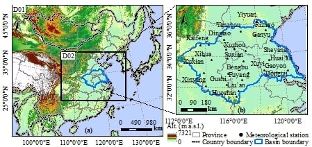
2.1. Study Area and Events

The HRB is one of seven major river basins in China; it is located between 110°–122 °E and 31°–37 °N (Figure 1b), and covers an area of 270,000 km². Most of the HRB region is vast plains, except for some mountains and foothills located at the western, southern, and northeastern HRB (as shown in Figure 1b). The mountain altitudes are normally 1000–2000 meters above the sea level (a.s.l.). The HRB is in the transitional zone between the abundant rainfall area of southern China and the arid area of northern China [46], belonging to the warm temperate and semi-humid monsoon region with an average temperature of 11–16 degrees centigrade and an average annual rainfall about 910 mm. The precipitation distribution within a year is very uneven. In the flood season (June–September), the total precipitation accounts for 50–80% of annual precipitation [47]. The heavy rainfall events that occur in the summer frequently cause disaster in this area. Across the basin, there is a gradual gradient in average annual precipitation from about 1000 mm in the southeast to less than 600 mm in the northwest, while the highest precipitation occurs in the inner mountain areas; this variation is a result of the topography [48]. A robust knowledge of the precipitation processes in the HRB is vital for local flood monitoring and water resource management.

To select the studied precipitation events, daily precipitation data from 30 meteorological stations in the HRB during 2015 were obtained from the China Meteorological Administration (CMA) and analyzed (Figure 2). Based on these CMA observations, the contributions of accumulated daily precipitation to the annual precipitation amounts at each meteorological station were calculated and sorted in decreasing order. As shown in Figure 2a, all 30 CMA stations received half of the total annual precipitation within seven days (Dingtao station) or 13 days (Huoshan station). This suggests that short-term heavy precipitation events are the main contributors to the total annual precipitation amount in the HRB. Therefore, we focused our studies on short-term heavy precipitation events. The mean monthly precipitation over the HRB in 2015 was also calculated, and is illustrated in Figure 2b. The results showed that the precipitation amount during the flood season of the HRB composed 58.23% of the annual amount at all of the stations. The mean monthly precipitation in June comprised the highest percentage (21.6%), and August had the second largest percentage (18.33%). However, because the WRF forcing data of the NCEP final analyses (FNL) ds083.3 was issued in July 2015, we selected one event from August. As shown in Figure 2c, a heavy rainfall event occurred on 9 August, when the daily precipitation at many CMA stations exceeded 50 mm, and the highest exceeded 160 mm; thus, we chose the rainfall event from 0000 UTC on 9 August to 1200 UTC on 11 August (hereafter referenced as event A) as our first case study. As shown in Figure 2b, the mean monthly precipitation in November was evidently the highest during the non-flood season. Therefore, we chose the rainfall event that occurred from 0000 UTC on 5 November to 1200 UTC on 7 November (hereafter referenced as event N) as our second case study. During event N, the average daily precipitation of the basin reached 22.1 mm, and that of a single CMA station (Rizhao) reached 66.6 mm. The two case studies (event A and event N; each spanned 60 h) represent the type of convection dominant precipitation events during a flood season, and extratropical cyclone-associated precipitation events during the non-flood season, respectively.

2.2. Study Data

2.2.1. Satellite Precipitation Products for Assimilation

In this study, two satellite-based precipitation data, including the TRMM 3B42 (version 7) and the GPM IMERG (final run), were applied as observation operators. Both were processed to collect six-hour accumulated precipitation data for assimilation into the WRF model.

TRMM was jointly launched by the National Aeronautics and Space Administration (NASA) and the Japan Aerospace Exploration Agency (JAXA) in 1997. TRMM 3B42 is one product of the TRMM Multi-satellite Precipitation Analysis (TMPA); it combines remote sensing data from various microwave and infrared sensors with the monthly gauge analysis from the Global Precipitation Climatology Centre (GPCC). TRMM 3B42 covers ±50 °N/S at spatiotemporal resolutions of 0.25° and 3 h [49]. After over 17 years of productive data acquisition, the observation instruments on TRMM were turned off on 8 April 2015. However, the actual termination of TRMM was not a substantive issue for its multi-satellite products in TMPA; therefore, the TRMM 3B42 data during our study periods are still available. Tang et al. [50] compared TRMM 3B42 with the gauge observations and found that the correlation coefficient (CC) over Mainland China reached 0.42 and 0.68 at its original three-hour and daily timescales, respectively; for the region encompassing the lower reaches of the Huaihe River, the CCs reached 0.43 and 0.71 at the three-hour and daily timescales, respectively.

As the replacement of TRMM, GPM has been providing next-generation global observations of rain and snow for more than three years. The observation system on the GPM comprises one core satellite and several constellation satellites, with a dual-frequency precipitation radar and a suite of microwave radiometers. The core observatory of the GPM was designed as an extension of TRMM’s highly successful rain-sensing package, which primarily focused on heavy to moderate rain over tropical and subtropical oceans [51]. A key advancement of the GPM over the TRMM is the extended capability to measure light rain (≤0.5 mm/hour) and falling snow, since the two types of precipitation account for significant proportions of precipitation at mid and high latitudes. GPM IMERG is the third-level precipitation product of GPM, which covers an area of ±60 °N/S with unprecedented resolutions of 0.1° and 30 min. Tang et al. [50] reported that when compared with the gauge observations, the CCs of GPM IMERG over Mainland China reached 0.53 and 0.71 at the hourly and daily timescales, respectively; for the region encompassing the lower reaches of the Huaihe River, the CCs reached 0.55 and 0.72 at the hourly and daily timescales, respectively.

2.2.2. Forcing Data for the WRF Model

To simulate the two heavy precipitation events over the HRB, the NCEP FNL datasets were applied to provide the WRF model with the initial states and lateral boundary conditions. Among the various NCEP FNL datasets, the commonly used 1.0° and six-hour FNL ds083.2 and the newly released 0.25° and six-hour FNL ds083.3 datasets were employed and compared. The one that performed better with the WRF model was used in the subsequent 4D-Var experiments. These two forcing data were composed of an underlying Global Forecast System (GFS) that was obtained from the Global Data Assimilation System (GDAS), which continuously collects observational data from the Global Telecommunications System (GTS) and other sources for many related analyses. The archived time series of the ds083.2 and ds083.3 datasets started on 30 July 1999 and 8 July 2015, respectively. Both of these datasets extended to a near-current date. They can be downloaded from the Research Data Archive at the National Center for Atmospheric Research (https://rda.ucar.edu/datasets/).

2.2.3. In Situ and Gauge-Corrected Data for Evaluation

To evaluate the precipitation results simulated by the WRF model and the WRF 4D-Var with TRMM 3B42 and GPM IMERG, two types of precipitation datasets were used as reference data. One was the in situ gauge observation dataset for daily precipitation; this data was obtained from the 30 meteorological stations in the HRB (Figure 1b) and provided by the CMA (hereafter referenced as CMA data). This dataset was collected as a benchmark for the point-scale evaluations. The accuracy of the CMA data was officially claimed to be approximately 100%, as before its release, it experienced a series of quality control assessments including a climate limit value check, station extreme value check, spatiotemporal consistency check, and other related checks (http://data.cma.cn/data/cdcdetail/dataCode/SURF_CLI_CHN_MUL_DAY_V3.0.html). When comparing with the CMA data, the simulated precipitation results from the WRF and the WRF 4D-Var models were changed to Beijing time, which is used in the CMA data. The other dataset was the gridded merged CMORPH data, which was used for the evaluation at the grid scale [52]. It is also released by the CMA, with spatiotemporal resolutions of 0.1° and hourly. The CMA generated the merged CMORPH data by applying the probability density function matching method and the optimal interpolation method. This dataset integrates with the following two data sources: (1) gauged hourly precipitation from more than 30,000–40,000 automatic weather stations in China after quality control; and (2) inverse precipitation products from the global CMORPH satellite, with resolutions of 30 min and 8 km provided by the Climate Prediction Center (USA). The merged CMORPH data have been opened to the public since 1 January 2008. This dataset covers mainland China, and its applied time zone was the same as that used in the WRF model, i.e., the UTC time zone. Its general error remains under 10%, and the errors in strong precipitation over sparsely-gauged areas are less than 20%. Its quality is better than that of other similar products in China (http://data.cma.cn/). When used for evaluation, the merged CMORPH data were resampled to the same spatial resolutions as those of the WRF domains (i.e., 27 km and 9 km) by the nearest neighborhood interpolation method. Moreover, to ensure evaluation quality, the coordinate system of the merged CMORPH data was transformed to be the same projected coordinate system as that used in the WRF model. It should be noted that for the grid-scale evaluation, assessments were only carried out over intersecting regions that encompassed the two WRF domains and the merged CMORPH data region since the latter only covered mainland China.

3. Methods

3.1. WRF Configuration, 4D-Var Methodology, and Experimental Design

3.1.1. WRF Configuration

To obtain precipitation at a finer resolution and reduce the computing quantity, a nested domain (Figure 1a) was applied in our WRF configuration. The outer domain (D01) was set around the HRB to be as large as possible to cover the important weather features of the HRB, which are probably caused by the Indian southwestern monsoon, the East Asian subtropical monsoon, and the Asian monsoon that originates from the Siberian high. However, D01 cannot be set to an unlimited large domain, as a large domain means more grids for calculation, which requires more computational resources. Therefore, we finally define D01 with grids of 180 * 155 and a 27-km resolution and set the inner domain (D02) to cover the whole HRB, with 226 * 175 grids and a 9-km resolution.

The physical configuration of the WRF model and its related dominant parameters were determined by obeying the rule that the configuration should incorporate the experiences obtained from comparable numerical modeling studies as much as possible, especially studies performed over the HRB. Moreover, a one-way nesting strategy was employed, since a nesting strategy was not decisive of the overall performance [53], and was not our research priority. The main configuration of the WRF model is listed in

Table 1. The main configuration of the Weather Research and Forecasting (WRF) model.

Map and Grids
Map projection	Lambert conformal
Center point of the domain	35.8 °N, 114 °E
Number of vertical layers	27
Horizontal grid resolution	27 km (D01), 9 km (D02)
Domain grid	180 * 155, 226 * 175
Static geographical fields time step	Standard dataset at a 30” resolution 150 s, 50 s from the United States Geological Survey (USGS)
Physical Parameterization Schemes
Cloud microphysics	WRF double-moment six scheme [54]
Long-wave radiation	Rapid Radiative Transfer Model (RRTM) [55]
Short-wave radiation	Dudhia scheme [56]
Land surface model	Noah land surface model (LSM) [57]
Planetary boundary layer	Yonsei University scheme [58]
Cumulus parameterization	New Grell–Devenyi 3 scheme [59] (except for the 9-km domain: no cumulus)

.

3.1.2. WRF Configuration

The incremental 4D-Var formulation, which is commonly used in operational systems [60,61,62,63], was utilized in the WRF 4D-Var data assimilation system. The incremental approach was designed to determine an analysis increment that minimized the cost function, which was defined as a function of the analysis increment instead of the analysis itself [64]. Mathematically, the WRF 4D-Var minimizes cost function J:

$$J=J_b+J_o+J_c$$

(1)

which includes quadratic measures of distance to the background, observation, and balanced solution. The background cost function term J_b is:

$$J_b=\frac{1}{2}{\left(x^n-x^b\right)}^T{B}^{-1}\left(x^n-x^b\right)$$

(2)

where the superscripts −1 and T denote the inverse and the adjoint of a matrix or a linear operator, respectively. The final analysis of WRF 4D-Var (i.e., after the last (n) outer loop occurs) is denoted as xⁿ. The background x^b has typically been a short-range forecast in previous analyses. B represents the background error covariance matrix.

The observation cost function term represents the quadratic measure of the distances between the analysis xⁿ and the forecast model M_k and the observation operator H_k and the observations y_k:

$$J_o=\frac{1}{2}{{\displaystyle \sum }}_{k=1}^K{\left\{H_k\left[M_k\left(x^n\right)\right]-y_k\right\}}^T{R}^{-1}\left\{H_k\left[M_k\left(x^n\right)\right]-y_k\right\}$$

(3)

When calculating the observation cost function J_o, a linear approximation is made, and the entire assimilation time window is split into K observation windows. The nonlinear observation operator H_k is approximately transformed into a tangent linear observation operator, and the nonlinear model M_k is also transformed into a tangent linear model. xⁿ denotes the guess vector, and xⁿ − xⁿ⁻¹ denotes the analysis increment. R represents the observation error covariance matrix.

The balancing cost function J_c measures the quadratic distance between the analysis and a balanced state, and it is expressed as follows:

$$J_c=\frac{1}{2}{\gamma }_{df}{\left[M_{\raisebox{1ex}{$N$}\!\left/ \!\raisebox{-1ex}{$2$}\right.}\left(x^n-x^{n-1}\right)-{{\displaystyle \sum }}_{i=0}^N{f}_i{M}_i\left(x^n-x^{n-1}\right)\right]}^T{C}^{-1}\left[M_{\raisebox{1ex}{$N$}\!\left/ \!\raisebox{-1ex}{$2$}\right.}\left(x^n-x^{n-1}\right)-{{\displaystyle \sum }}_{i=0}^N{f}_i{M}_i\left(x^n-x^{n-1}\right)\right]$$

(4)

where N represents the total number of integration steps over the assimilation window, and γ_df represents the weight assigned to the J_c term. f_i is the coefficient for the digital filter [65,66]. C is a diagonal matrix containing variances of wind, temperature, and dry surface pressure, with values of (3 m/s)², (1 K)², and (10 hPa)², respectively.

3.1.3. Experimental Design

In this study, two series of experiments were carried out over the HRB. The first series of experiments, which are labeled the CTL experiments in this manuscript, were performed with the WRF model. They were carried out to choose the most optimal forcing data for the WRF model and determine the control experiments for the subsequent 4D-Var assimilation study. According to the different applied forcing data and the different study events, the CTL experiments were labeled from CTL1 to CTL4 (

Table 2. Designs of the WRF control (CTL) experiments and the WRF data assimilation (DA) experiments.

No.	Studied Event	Forcing Data	No.	Studied Event	Assimilated Data
CTL1	Event A	FNL ds083.2	DA1	Event A	TRMM 3B42
CTL2		FNL ds083.3	DA2		GPM IMERG
CTL3	Event N	FNL ds083.2	DA3	Event N	TRMM 3B42
CTL4		FNL ds083.3	DA4		GPM IMERG

). The second series of experiments utilized the 4D-Var via direct assimilation of TRMM 3B42 and GPM IMERG. They were referred to as the DA experiments (Table 2). For the DA experiments, the background error covariance matrices, B, for August and November in 2015 were separately generated with one-month ensemble forecasts every 12 h using the NMC method [67]. Meanwhile, one variable, named “eps”, was set to 0.0001 to make the WRF DA convergence criterion more stringent. In addition, by considering the impacts of the WRF spin-up [61,68,69], we utilized the WRF forecast during the first 12-hour period of each CTL experiment as the first guess of the 4D-Var assimilation in each DA experiment. Thus, the simulation period for each DA experiment was reduced to 48 h. For each 24 h segment of the 48 h period, there was one WRF 4D-Var model that provided the initial and boundary conditions for the other WRF model with a forecast period of 24-hour cycles; this cycling mode was used to connect the simulations during the entire 48 h. With the application of 32 GB of memory on eight nodes and 16 CPU/nodes on the supercomputer used in our study, each WRF 4D-Var that ran over a six-hour time window took approximately 12 h. Limited by the available computational resources, 4D-Var was only employed in D01. Given the problem of the WRF spin-up, the first 12 h of the CTL experiments were not included in the following evaluations. Therefore, in this study, the evaluation periods for both the CTL experiments and DA experiments spanned from 1200 UTC on 9 August to 1200 UTC on 11 August in 2015 for event A, and from 1200 UTC on 5 November to 1200 UTC on 7 November in 2015 for event N.

3.2. Evaluation Metrics

To evaluate the simulated precipitation results of the CTL and DA experiments, we applied two categories of metrics, which are shown in

Table 3. Statistical metrics applied in the evaluations *.

Statistical Metrics	Equation	Perfect Value
Mean Error (ME; unit: mm)	$ME=\frac{1}{N}{\displaystyle {\displaystyle \sum }_{i=1}^N}\left(P_{P,i}-P_{O,i}\right)$	0
Relative Error (RE)	$RE=\frac{{{\displaystyle \sum }}_{i=1}^N\left(P_{P,i}-P_{O,i}\right)}{{{\displaystyle \sum }}_{i=1}^N{P}_{O,i}}$	0
Root Mean Square Error (RMSE; unit: mm)	$RMSE=\sqrt{\frac{1}{N}{\displaystyle \sum }_{i=1}^N{\left(P_{P,i}-P_{O,i}\right)}^2}$	0
Correlation Coefficient (CC)	$CC=\frac{{{\displaystyle \sum }}_{i=1}^N\left(P_{P,i}-\acute{P_{P,i}}\right)\left(P_{O,i}-\acute{P_{O,i}}\right)}{\sqrt{{{\displaystyle \sum }}_{i=1}^N{\left(P_{P,i}-\acute{P_{P,i}}\right)}^2{{\displaystyle \sum }}_{i=1}^n{\left(P_{O,i}-\acute{P_{O,i}}\right)}^2}}$	1
Bias Score (BIAS)	$BIAS=\frac{\left(A+B\right)}{\left(A+C\right)}$	1
False Alarm Ratio (FAR)	$FAR=\frac{B}{\left(A+B\right)}$	0
Probability of Detection (POD)	$POD=\frac{A}{\left(A+C\right)}$	1
Probability of False Detection (POFD)	$POFD=\frac{B}{\left(B+D\right)}$	0
Heidke Skill Score (HSS)	$HSS=\raisebox{1ex}{$\left(s-S_{Ref}\right)$}\!\left/ \!\raisebox{-1ex}{$\left(S_{Perf-S_{Ref}}\right)$}\right.$ $S=\frac{\left(A+D\right)}{N}$ $S_{Ref}=\frac{\left[\left(A+B\right)\left(A+C\right)+\left(B+D\right)\left(C+D\right)\right]}{N^2}$	1

* P_P,i and P_O,i denote the predicted and observed precipitation values of the i grid, where $\acute{P_{P,i}}$ and $\acute{P_{O,i}}$ are their means, respectively. A represents the precipitation predicted by the WRF model and observed by the reference data; B represents the precipitation predicted by the WRF model but not observed by the reference data; C represents the precipitation not predicted by the WRF model but observed by the reference data; and D represents the precipitation not predicted by the WRF model and not observed by the reference data.

. The first category of metrics contained the mean error (ME), the relative error (RE), the root mean square error (RMSE), and the CC, which were used to describe the errors, deviations, and correlations between the simulated precipitation and the reference precipitation at the point scale. The second category of metrics contained skill scores commonly used in meteorological studies, including the bias score (BIAS), the false alarm ratio (FAR), the probability of detection (POD), the probability of false detection (POFD), and the Heidke skill score (HSS). These skill scores were constructed based on a contingency table [70] and applied in the evaluation at the grid scale. BIAS is an indicator of how well the model predicts the number of occurrences of an event. FAR indicates the fraction of forecasts detected by the WRF model that turns out to be wrong. POD represents the ratio of correct forecasts to the number of events that occurred, which is commonly known as the hit rate. POFD represents the faction of false alarms to the total number of events that did not occur. HSS is one of the most frequently used and comprehensive skill scores for summarizing square contingency tables and combining the characteristics of hints and random detections. Considering that the detection accuracy of the CMA ground observation was 0.1 mm/day, the rain/no rain threshold was set to 0.1 mm in this study.

4. Results

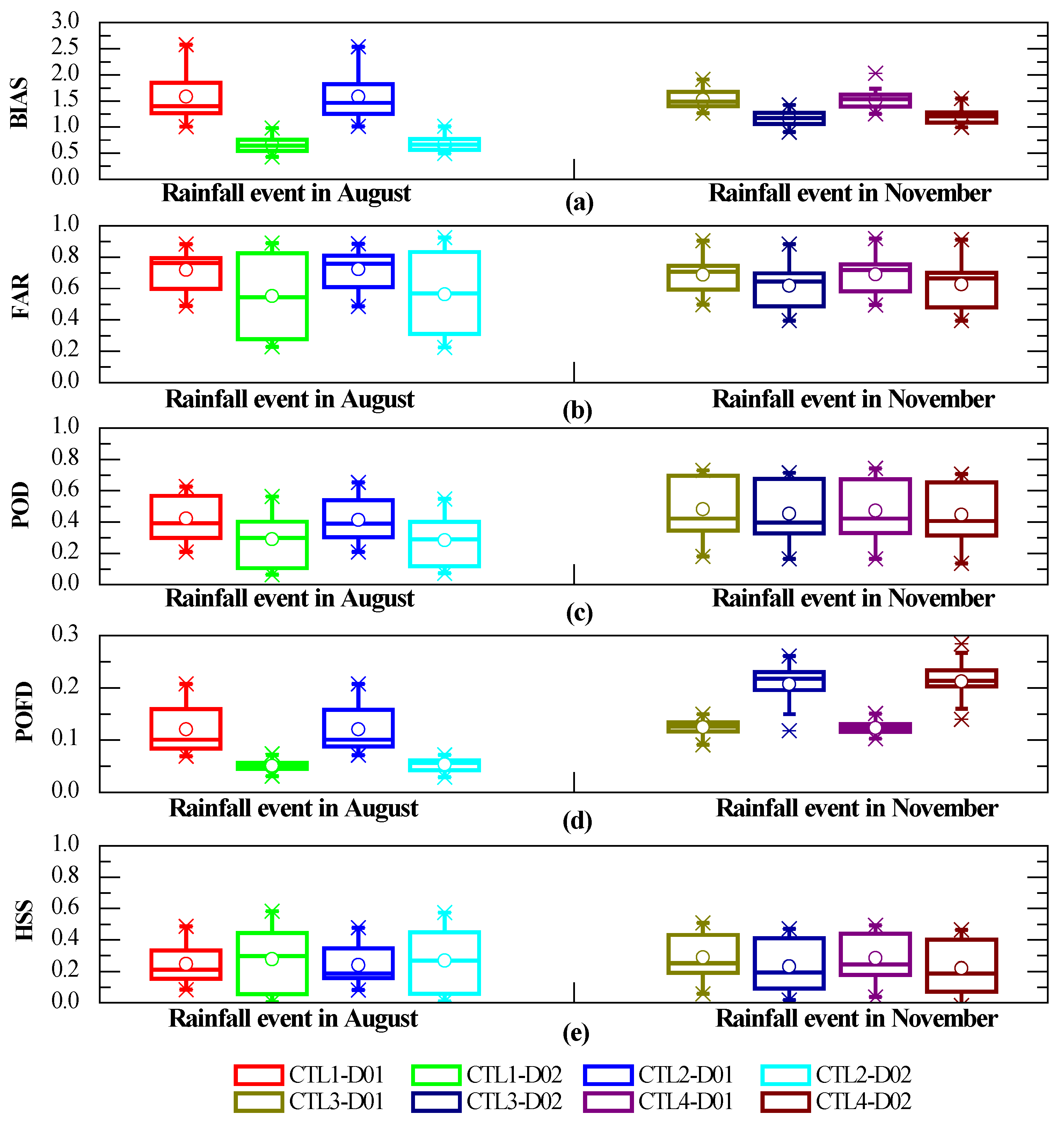
4.1. Evaluation of Simulated Precipitation in the CTL Experiments

4.1.1. Evaluation of Simulated Precipitation in the CTL Experiments at the Point Scale

To evaluate the precipitation simulated by the WRF model at the point scale, the error indices of ME, RE, CC, and RMSE were used. Precipitation values in D01 and D02 were both extracted from grids located closest to the CMA stations, then accumulated into daily values and compared against the daily in situ CMA data. As delineated in Figure 3, for both event A and event N, the values of ME and RE in D01 and D02 were positive, which indicated that the WRF-predicted precipitation results were generally overestimated. Although the CC values of event N were lower than those of event A, the points that represented the relationship between the station precipitation and the predicted precipitation was evidently much closer to the 1:1 line for event N (Figure 3b) than that for event A (Figure 3a). Moreover, the values of ME, RE, and RMSE for event N were also lower than those for event A. This means that the predicted precipitation results for event N showed better agreement with the CMA observations than those for event A. In addition, the error metrics for the simulated precipitation from D02 were generally comparable to those from D01, which indicated that the resolution increase for precipitation from 27 km (D01) to 9 km (D02) was realized through the nested domain at a very slight accuracy reduction cost at the point and daily scales. For the variations made by different forcing data, there appeared to be some slight negative changes in the ME, RE, CC, and RMSE values from CTL4 to CTL3, but the CCs of CTL 2 were only 0.01 lower than those of CTL1, and the ME, RE, and RMSE values of CTL2 were evidently much lower than those of CTL1. Therefore, we conclude that the WRF performance driven by the FNL ds083.3 dataset outperformed that driven by the ds083.2 dataset at the daily and point scales.

4.1.2. Evaluation of the Simulated Precipitation in the CTL experiments at the Grid Scale

To make the evaluations of the simulated precipitation more complete, we also compared the simulated precipitation from the CTL experiments with the hourly merged CMORPH data. The skill scores of BIAS, FAR, POD, POFD, and HSS were used to quantify the assessment. The evaluated results are displayed in Figure 4. It is observed that the box lengths of BIAS, FAR, and POFD for event N were much shorter than those for event A, which indicated lower deviations and better performances for the simulation of event N. This finding was consistent with the evaluated results at the daily and point scales. Thus, we conclude that the WRF performance for event N was better than that for event A. This was probably attributed to the over or underestimation of the WRF model for localized extreme precipitation intensities when simulating strong convective precipitation events.

By comparing the evaluation results between D01 and D02, it is found for event A that the values of BIAS over D02 were much closer to 1 than those for event N; the mean values of FAR and POFD over D02 were much lower, and the maximum and mean values of HSS over D02 were higher. For the rainfall in event N, although the comprehensive index values of HSS over D02 were slightly lower than those over D01, the BIAS values over D02 were much closer to 1 than those over D01, and the FAR values also decreased more over D02 than those over D01. Thus, advantages in the WRF improvement regarding spatial resolution were conveyed both in convective and non-convective rainfall events at the grid and hourly scales.

Based on the above evaluations, the forcing data of NCEP FNL ds083.3 dataset were selected to drive the following WRF 4D-Var experiments. The CTL2 experiment was utilized as the reference for DA1 and DA2 (event A), and the CTL4 experiment was determined as the reference for DA3 and DA4 (event N).

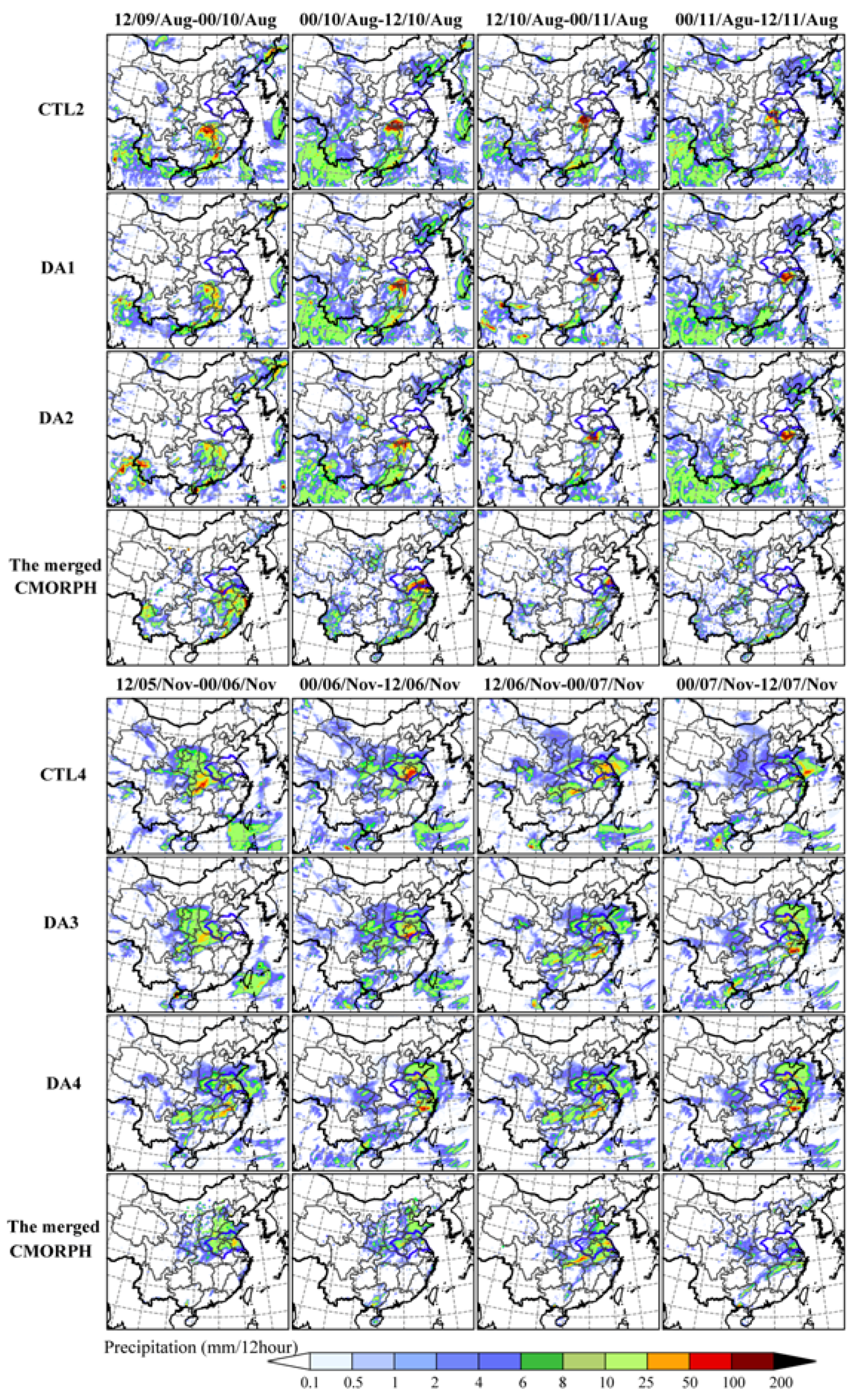
4.2. Evaluation of the Simulated Precipitation in the DA Experiments

The DA experiments output precipitation values with spatiotemporal resolutions of 27 km and 150 s in D01, and 9 km and 50 s in D02. Figure 5 shows the spatial patterns of the 12-hour accumulated precipitation extracted from the reference CTL experiments, the DA experiments and the merged CMORPH dataset over a subset of the D01 domain. It is clear in Figure 5 that the CTL2 experiment captures the shift in precipitation during event A over the HRB from the southwest to the northeast, and the CTL4 experiment also captures the shift in precipitation during event N over the HRB from the west to the east of the HRB. However, compared with the merged CMORPH data, which served as the true measurements at the grid scale, the spatial distributions and the amounts of simulated precipitation in CTL2 and CTL4 were much wider and larger than those reflected in the merged CMORPH dataset. For each 24-hour period, these discrepancies between the simulated precipitation and the merged CMROPH data became more evident in the second 12-hour period than those in the first 12-hour period, which may be related to the error accumulations when the WRF model was running. It can also be found in Figure 5 that the simulated precipitation after assimilation with TRMM 3B42 and GPM IMERG was more agreeable with the merged CMORPH dataset.

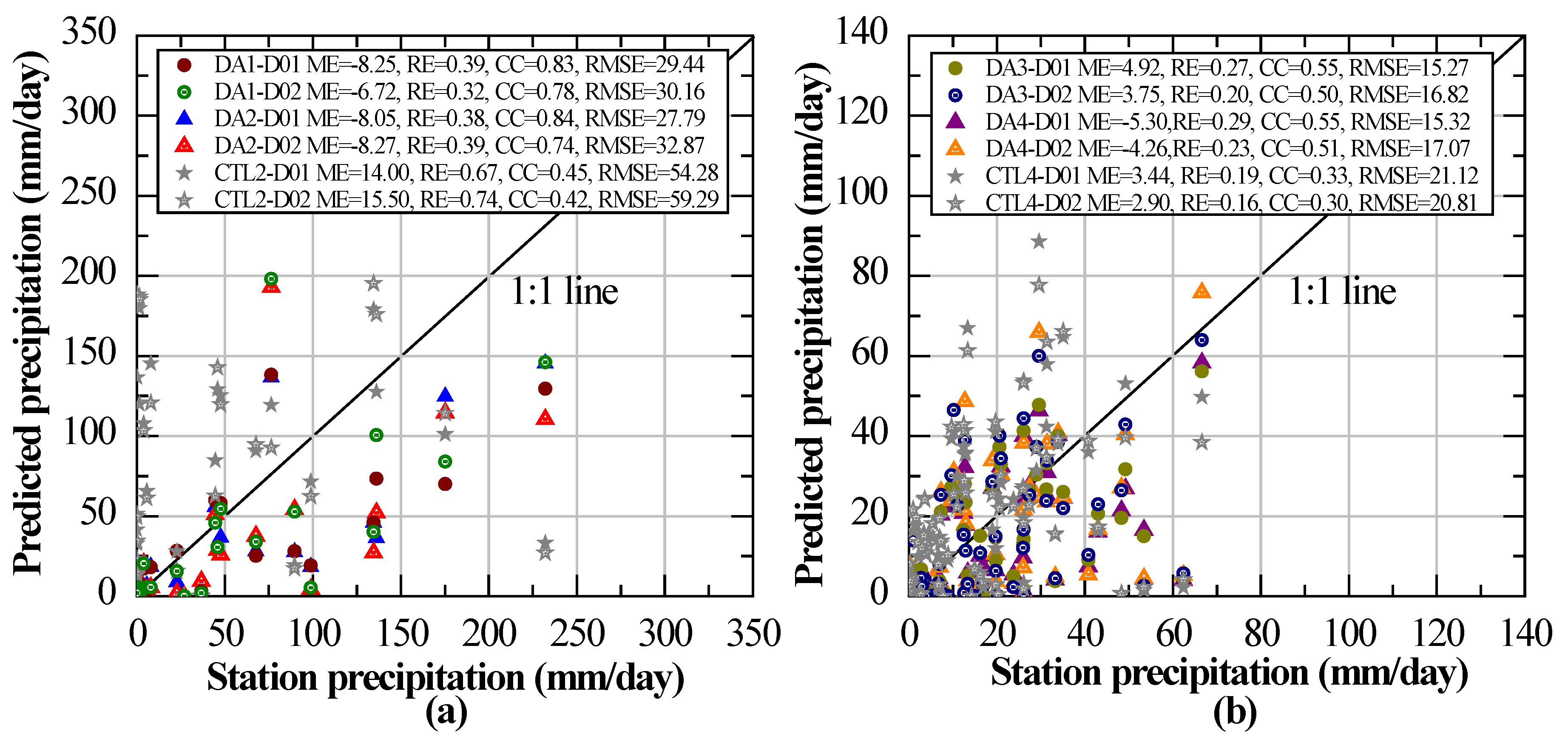
4.2.1. Evaluation of Simulated Precipitation in the DA Experiments at the Point Scale

To evaluate the simulated precipitation in the DA experiments at the point scale, precipitation values were extracted from the grids closest to the CMA stations from the DA simulations, which were accumulated into daily values and compared against the daily CMA data. The evaluated error indices of ME, RE, CC, and RMSE for the control experiments and the DA experiments are displayed in Figure 6. As shown in Figure 6a, the application of 4D-Var to event A had an obvious change in simulated precipitation via CLT2 from over-forecasting (above the 1:1 line) to under-forecasting (below the 1:1 line). This variation can also be found in the numerical changes in ME from positive values to negative values. For event N (Figure 6b), the MEs changed differently. The MEs for DA3 were still positive (indicating over-forecasting), and the MEs for DA4 were negative (indicating under-forecasting). This means that after assimilating GPM IMERG, WRF precipitation outputs tend to be lower than those from the corresponding CTL experiments for both event A and event N. By assimilating with the remotely sensed precipitation products, the RMSEs of all of the DA experiments all significantly decreased, which indicated reduced deviations in the precipitation outputs of the WRF 4D-Var. Moreover, the CCs of the DA experiments all significantly increased. The biggest CC increase for event A was 0.39 (from CTL2-D01 to DA2-D01) and 0.22 for event N (from CTL4-D01 to DA4-D01). These positive variations manifested improvements in the precipitation simulations due to the assimilation of TRMM 3B42 and GPM IMERG onto WRF at the daily and point scales.

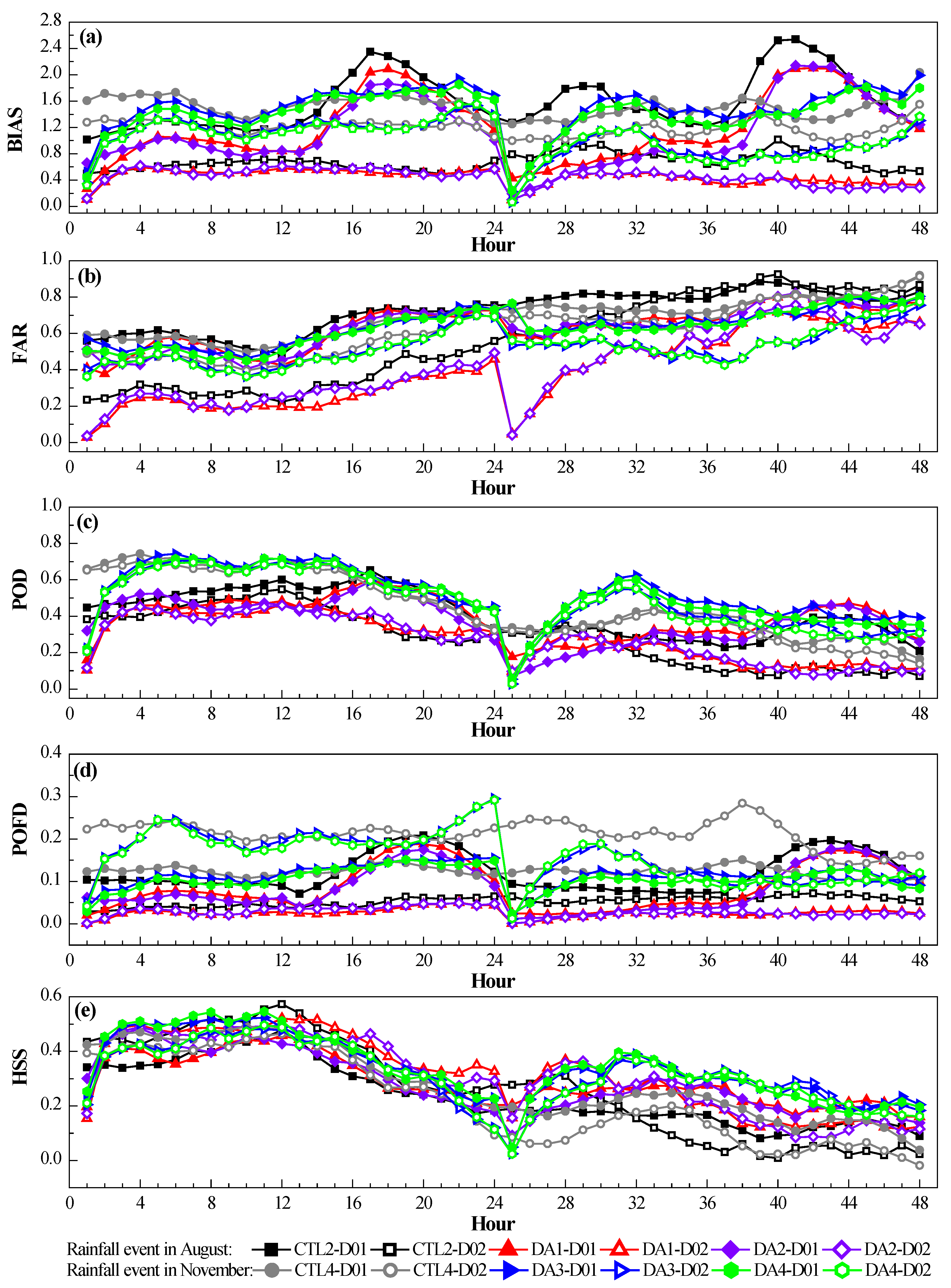
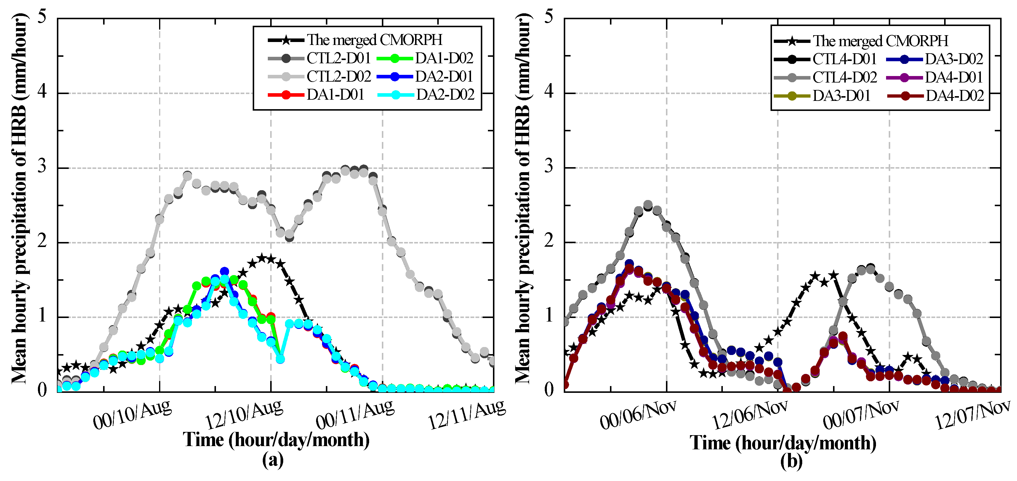
4.2.2. Evaluation of Simulated Precipitation in the DA experiments at the Grid Scale

The simulated precipitation results of the DA experiments in D01 and D02 were processed into hourly values and evaluated with the grid data (i.e., the hourly merged CMORPH data). The evaluations were quantified by the skill scores of BIAS, FAR, POD, POFD, and HSS. These skill scores for the hourly precipitation from the CTL2, CTL4, and DA experiments changed with time during the 48 h in each experiment (Figure 7). On the whole, for the reason of error accumulation during the simulations, the FAR values showed increasing tendency with time, the values of POD and HSS presented decreasing tendency with time, the values of BIAS and POFD fluctuated with time, and the amplitudes were weakened by the application of 4D-Var in DA experiments. Looking into the HSS variation, for the reason of 4D-Var data assimilation, the HSS values for the hourly precipitation predictions increased at first, but as time passed, they decreased because of the error accumulation during the simulations. Moreover, there appear abrupt changes between the 24th hour and the 25th hour in Figure 7a–e. These sudden variations were caused by the newly initial and boundary conditions accompany with the start of the second 24-hour forecast in each DA experiment.

Besides, it is also seen in Figure 7 that in the same domains, all of the values of BIAS, FAR, and POFD for the DA experiments are primarily lower than those in the CTL experiments. This suggests that the 4D-Var-assimilated TRMM 3B42 or GPM IMERG can effectively reduce several false alarms regarding rainfall occurrences. It is noteworthy that the variations in hit rates, which were indicated by the PODs, were different between event A and event N (Figure 7c). When comparing CTL2-D01 and CTL2-D02, the POD average values of DA1-D01, DA1-D02, DA2-D01, and DA2-D02 were reduced by 0.02, 0.01, 0.04, and 0.01, respectively. For event N, the PODs of DA3 and DA4 all remarkably improved compared with those of CTL4. These different variations in POD were probably attributed to the different precipitation mechanisms of event A and N and the imperfection of WRF in predicting extreme local precipitation. Regardless, the comprehensive scores of HSS for the DAs finally improved. In comparison with the mean hourly HSS values for the reference CTL experiments, the HSS mean values of DA1-D01, DA1-D02, DA2-D01, DA2-D02, DA3-D01, DA3-D02, DA4-D01, and DA4-D02 increased by 0.05 (0.28), 0.05 (0.32), 0.04 (0.28), 0.04 (0.31), 0.05 (0.34), 0.09 (0.31), 0.06 (0.34), and 0.09 (0.31), respectively (the HSS values are in parentheses). This definitely demonstrates the positive improvements in the precipitation simulations that were made by the 4D-Var assimilation with TRMM 3B42 and GPM IMERG via the WRF model at the grid and hourly scales. Moreover, it can be concluded that the improvements in WRF 4D-Var for event A mainly benefited from the corrections of the false alarms for non-occurrences, since the POD values for DA1 and DA2 decreased, but their BIASs, FARs, and POFDs also reduced, which finally improved their HSSs. For event N, the reductions in BIASs, FARs, and POFDs were minor, but the PODs experienced evident improvements, and the HSSs finally became better than those of CTL4.

Considering precipitation applications in a hydrological basin, the simulated precipitation results of the DA experiments in the HRB were specifically evaluated; they were extracted, accumulated and spatially averaged. Figure 8 shows the hourly mean precipitation values of the basin via the CTL2, CTL4, and DA experiments during the studied 48 h. As shown in Figure 8, the agreements between the DAs’ simulated precipitation and the merged CMORPH estimations were better than those between the CTL simulated results and the merged CMORPH estimations. Nevertheless, it should be noted that the impact of the WRF 4D-Var was not always consistent throughout the whole forecast period. For each 24-hour simulation, the mean precipitation of the basin via the DAs had the greatest agreement with the merged CMORPH estimations at the beginning (about the first 12 h). During the next 6 h, the mean precipitation values of the basin also maintained relatively good consistency with the merged CMORPH data. However, in the following hours, the predictions showed evident deviations from the merged CMORPH estimations. The reduction in the positive impact on the precipitation simulations suggested a time interval for the efficiency of the WRF 4D-Var. This may be related to the inevitable errors that accumulate while the WRF 4D-Var DA system is running [53]. Moreover, when we applied the cycling mode, the initial conditions of the subsequent 24-hour forecast were provided by the previous 24-hour forecast; this caused error accumulation from the first 24-hour simulation, and as a result, the WRF 4D-Var performance for the subsequent 24 h became generally worse than that for the first 24 h.

5. Discussions

5.1. WRF Sensitivity to Different Rainfall Events, Forcing Data, and Spatial Resolutions

To quantitatively assess the WRF sensitivity to different rainfall events, different forcing data and spatial resolutions, the error indices of ME, RE, CC, and RMSE and the skill scores of BIAS, FAR, POD, POFD, and HSS for the CTL experiments were inter-compared and are displayed in Figure 9a,b, respectively. Both the sharp decreases in ME, RE, and RMSE from CTL1-2 to CTL3-4 (Figure 9a) and the evident BIAS value much closer to 1 (Figure 9b) demonstrated a better WRF performance for event N than that for event A. This finding is consistent with that concluded by Lin et al., [42], where they found that the WRF model was relatively harder to use when forecasting convective and dominant precipitation events than precipitation events caused by extratropical cyclones.

The impacts of different forcing data on the WRF precipitation simulations were well reflected in the error indices at the daily and point scales. As shown in Figure 9a, the CCs of CTL2 over D01 and D02 were both 0.01 lower than the CCs of CTL1. However, the ME, RE, and RMSE values of CTL2 significantly decreased by 22.61%, 22.09%, and 12.63% compared with those of CTL1_D01, respectively, and decreased by 15.53%, 14.94% and 11.81% compared with those of CTL1_D02, respectively. This indicated that significant improvements were made by using forcing data ds083.3 for event A. For event N, contrasted with CTL3, the CCs of CTL4 decreased by 0.03 in D01 and 0.04 in D02. The ME, RE, and RMSE values of CTL4_D01 slightly increased by 1.03 mm, 0.06 mm, and 2.31 mm respectively, compared with those of CTL3_D01. The values of CTL4-D02 increased by −0.07 mm, 0.00 mm, and 0.83 mm, respectively, compared to those of CTL3_D02. These results indicated that slightly negative impacts of ds083.3 were found when predicting non-convective precipitation. These differences in the error indices caused by different forcing data suggested that the WRF model is very sensitive to its initial and lateral boundary conditions, especially for convective precipitation. Considering the notable positive improvements caused by ds083.3 for the simulation of convective precipitation, the slightly negative impacts of ds083.3 on the simulation of non-convective precipitation were omitted from this study. Therefore, we considered forcing data ds083.3 to be better than ds083.2 to drive the WRF model.

As shown in Figure 9b, the mean hourly BIASs and FARs of the CTLs over D02 showed more evident decreases than those over D01, and these reductions of CTL1 and CTL2 were especially remarkable. The POD values over D02 were slightly lower than those over D01 for event A, but the mean hourly PODs for event N over D01 and D02 were nearly the same. For event A, the POFDs in D02 were visually lower than those in D01, and the comprehensive HSSs in D02 were higher than those in D01. For event N, the HSSs in D02 were lower than those in D01, while clearly lower values of the BIASs and FARs over D02 indicated some improvements in the reduction of false predictions. Hence, we conclude that the improvement of spatial resolution (from 27 km to 9 km) in the WRF model has an evident positive impact on precipitation predictions for strong convection-dominated rainfall events, and slightly negative impacts on the predictions of rainfall events associated with extratropical cyclones. Considering the practical need for finer spatial resolutions and the overall better performances over the D02, we recognize that the WRF performance is better over D02 than that over D01.

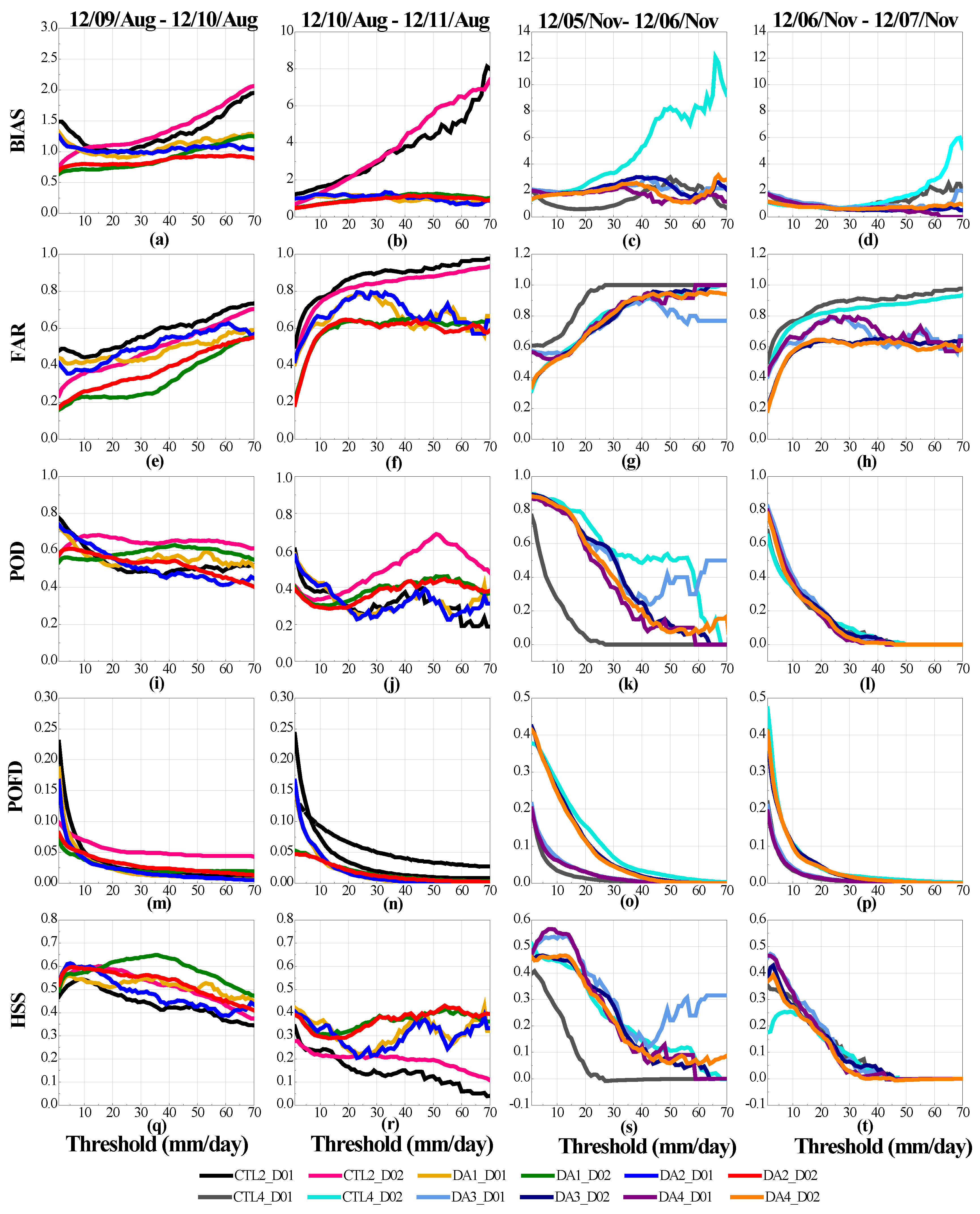
5.2. The Effectiveness of WRF 4D-Var at Different Thresholds and Time

To examine the WRF 4D-Var effectiveness in detail, the simulated daily precipitation from the CTL2, CLT4, and DA experiments at different thresholds ranging from 1 mm/day to 70 mm/day were evaluated with the daily merged CMORPH data. The assessments were quantified with the skill scores of BIAS, FAR, POD, POFD, and HSS. As shown in Figure 10, the performances of the WRF and WRF 4D-Var models decreased as the precipitation threshold increased. The predictions for strong precipitation events greater than 50 mm/day were severely over-forecasted in CTL2 and CTL4, as their BIASs mostly surpassed 2 and even reached 12 (Figure 10c). After assimilating the satellite precipitation products, over-forecasting was controlled, as the values of BIAS and FAR for the strong precipitation event obviously decreased (Figure 10a–d). As shown in Figure 10q,s, the HSSs of DA1-D02 and DA3-D01 for precipitation exceeding 40 mm/day were evidently much larger than those in other experiments, which suggested that the resultant heavy precipitation event assimilated with TRMM 3B42 was more accurate than that assimilated with GPM IMERG during the first day of each simulation. For the second day, these two simulated precipitation results tended to be over-forecasted. For light rain, the simulated precipitation results of DA2 and DA4 were better than those of DA1 and DA3. The BIASs for both DA2 and DA4 were generally much closer to 1, and they had lower values of FAR and POFD and higher values of POD and HSS. This was mainly attributed to the key advancement of the GPM over the TRMM, because the GPM has a better capability of measuring light rain; this is because its core observatory carried the first spaceborne Ku/Ka band dual-frequency precipitation radar, which is more sensitive to light rain rates [50].

Looking into the time interval issues regarding the effectiveness of the 4D-Var, which was mentioned in Section 4.2, the 12-hour accumulated precipitation of the DA experiments, the CTL2 and the CTL4 were evaluated with the skill scores. The increments of the skill scores between the DA experiments and its corresponding control experiment were analyzed. As portrayed in Figure 11, the increments of BIAS, FAR, and POFD at the first and third 12-hour periods exhibited more extensive decreases than those during the second and fourth 12-hour periods, especially for event A, which is represented with red lines. The PODs for event A reduced, but those for event N increased. In Figure 11e, most of the HSS increments in the first and third 12-hour periods were higher than those in the second and fourth 12-hour periods. Thus, we conclude that substantial improvements via the WRF 4D-Var with TRMM 3B42 and GPM IMERG can be sustained for approximately 12 h.

5.3. Comparison of the 4D-Var Performance Assimilated with TRMM 3B42 and GPM IMERG

To comprehensively compare the 4D-Var performance after assimilation with TRMM 3B42 and GPM IMERG, normalized Taylor diagrams [71] were used to compare the spatial patterns of daily and 48-hour (i.e., the whole study period) precipitation data between the simulations of the DA, CTL experiments, and the merged CMORPH data. The Taylor diagrams and are shown in Figure 12.

For the first day (Figure 12a), DA2 agrees the best with the merged CMORPH data, as the two points delegated DA2_D01 and DA2_D02 are the closest to the point labeled as REF in the figure, and the two points also show the highest correlation coefficients. Simultaneously, they almost have the same standard deviations as those of the merged CMORPH estimations, since they are located on the bold dashed line. For DA2-D01 and DA2-D02, their correlation coefficients are 0.692 and 0.663, respectively, and both their RMSEs occur at approximately 0.75 mm. DA3 and DA4 slightly differ in performance, as their representative points are very close to each other. For the performances on the second day (shown in Figure 12b), CTL2 exhibits a remarkable departure from the REF point, as simulation errors accumulated from the first day to the second day during the WRF was running. These performances rank from best to worst for event A as follows: DA2-D02, DA1-D02, DA1-D01, and DA2-D01. For event N, the results of DA3 and DA4 over D01 and D02 are almost the same. It is clear in Figure 12c that DA2 evidently outperforms DA1. Thus, we conclude that the WRF 4D-Var with GPM IMERG generally outperforms the WRF 4D-Var with TRMM 3B42.

6. Conclusions

To reduce data acquisition difficulty for precipitation in hydrological studies and obtain independent, consecutive, and high-resolution precipitation data, we used a 4D-Var data assimilation method to assimilate the remotely sensed precipitation products of the TRMM 3B42 and GPM IMERG into the atmospheric WRF model. By focusing on two heavy precipitation events that occurred during the flood and non-flood seasons over the HRB in 2015, CTL experiments were first carried out to choose the best forcing data for the WRF model and determine the control experiment for the subsequent DA experiments. Then, DA experiments were carried out to investigate the feasibility and efficiency of the GPM IMERG to be assimilated into the WRF model with the 4D-Var method, and the 4D-Var performances assimilating with the GPM IMERG and the TRMM 3B42 were compared as well. All of the simulated precipitation values from the CTL experiment and the DA experiment were evaluated with in situ CMA observations and hourly merged CMORPH data.

CTL experiments were performed based on the WRF model with different forcing data and for different events. The assessment of the simulated precipitation in the CTL experiments found that when predicting heavy rainfall events over the HRB, the WRF performance for event N, which represented non-convective precipitation, outperformed the performance for event A, which represented convective precipitation. Moreover, the simulated precipitation generated by forcing data ds083.3 and the output from nested domain D02, which had a higher spatial resolution (9 km), could generally yield better agreement with the in situ CMA data and the merged CMORPH data.

DA experiments were carried out with forcing data ds083.3. The 4D-Var performances that were assimilated with TRMM 3B42 and GPM IMERG based on the WRF model were evaluated in detail. The simulated precipitation results of the DA experiments were assessed at spatial scales of D01, D02, and the HRB, and at hourly, 12-hour, daily, and 48-hour timescales. The evaluation results showed that (1) the 4D-Var with both the TRMM 3B42 and GPM IMERG based on the WRF model could significantly improve the precipitation simulations. The improvements made by GPM IMERG generally outperformed those made by TRMM 3B42, as GPM IMERG was more sensitive to light rain (≤0.5 mm/hour), which accounted for significant portions of the precipitation occurrences at mid and high latitudes. (2) For event A, the enhancement of simulated precipitation was mainly attributed to the corrections of false alarms for non-occurrences. For event N, this improvement was primarily due to more accurate forecasting of these occurrences. The accuracy enhancement for event A was larger than that for event N. (3) The accuracy improvement in simulated precipitation over D01 (27 km) by 4D-Var could be effectively achieved over D02 (9 km); assimilation in D01 and downscaling to D02 with a nested domain based on the WRF model could provide an effective way to obtain finer-resolution precipitation forecasts. (4) Due to error accumulations in the WRF running, essential improvements made by the 4D-Var were maintained for approximately 12 h; it was also not recommended to use the cycling mode for error accumulations in the WRF model.

Further studies can be conducted to deepen the understanding of the 4D-Var algorithm from the following aspects: (1) investigating the performance of a longer duration precipitation simulation; (2) assimilating more remotely sensed precipitation products into other NWP models; and (3) analyzing the sensitivity of the WRF 4D-Var to background errors, which would be worthwhile for future studies.

References

1. Palmer, T.N.; Ralsanen, J. Quantifying the risk of extreme seasonal precipitation events in a changing climate. Nature 2002, 415, 512–514. [Google Scholar] [CrossRef] [PubMed]
2. Groisman, P.Y.; Karl, T.R.; Easterling, D.R.; Knight, R.W.; Jamason, P.F.; Hennessy, K.J.; Suppiah, R.; Page, C.M.; Wibig, J.; Fortuniak, K.; et al. Changes in the probability of heavy precipitation: Important indicators of climatic change. Clim. Chang. 1999, 42, 243–283. [Google Scholar] [CrossRef]
3. Groisman, P.Y.; Knight, R.W.; Karl, T.R. Heavy precipitation and high streamflow in the contiguous United States: Trends in the twentieth century. Bull. Am. Meteorol. Soc. 2001, 82, 219–246. [Google Scholar] [CrossRef]
4. Zhang, W.; Villarini, G. Heavy precipitation is highly sensitive to the magnitude of future warming. Clim. Chang. 2017, 145, 249–257. [Google Scholar] [CrossRef]
5. Zeng, J.Y.; Li, Z.; Chen, Q.; Bi, H.Y.; Qiu, J.X.; Zou, P.F. Evaluation of remotely sensed and reanalysis soil moisture products over the Tibetan Plateau using in-situ observations. Remote Sens. Environ. 2015, 163, 91–110. [Google Scholar] [CrossRef]
6. Zeng, J.Y.; Chen, K.S.; Bi, H.Y.; Chen, Q. A Preliminary Evaluation of the SMAP Radiometer Soil Moisture Product over United States and Europe Using Ground-Based Measurements. IEEE Trans. Geosci. Remote Sens. 2016, 54, 4929–4940. [Google Scholar] [CrossRef]
7. Pan, X.D.; Li, X.; Cheng, G.D.; Hong, Y. Effects of 4D-Var data assimilation using remote sensing precipitation products in a WRF Model over the complex terrain of an arid region river basin. Remote Sens. 2017, 9, 693. [Google Scholar] [CrossRef]
8. Alemohammad, S.H.; McLaughlin, D.B.; Entekhabi, D. Quantifying precipitation uncertainty for land data assimilation applications. Mon. Weather Rev. 2015, 143, 3276–3299. [Google Scholar] [CrossRef]
9. Ward, E.; Buytaert, W.; Peaver, L.; Wheater, H. Evaluation of precipitation products over complex mountainous terrain: A water resources perspective. Adv. Water Resour. 2011, 34, 1222–1231. [Google Scholar] [CrossRef]
10. Chen, Y.J.; Ebert, E.; Walsh, K.E.; Davidson, N. Evaluation of TRMM 3B42 precipitation estimates of tropical cyclone rainfall using PACRAIN data. J. Geophys. Res. Atmos. 2013, 118, 2184–2196. [Google Scholar] [CrossRef]
11. McCabe, M.F.; Rodell, M.; Alsdorf, D.E.; Miralles, D.G.; Uijlenhoet, R.; Wagner, W.; Lucieer, A.; Houborg, R.; Verhoest, N.E.C.; Franz, T.E.; et al. The future of earth observation in hydrology. Hydrol. Earth Syst. Sci. 2017, 21, 3879–3914. [Google Scholar] [CrossRef]
12. Steiner, M.; Smith, J.A.; Burges, S.J.; Alonso, C.V.; Darden, R.W. Effect of bias adjustment and rain gauge data quality control on radar rainfall estimation. Water Resour. Res. 1999, 35, 2487–2503. [Google Scholar] [CrossRef]
13. Lorenz, C.; Kunstmann, H. The hydrological cycle in three state-of-the-art reanalyses: Intercomparison and performance analysis. J. Hydrometeorol. 2012, 13, 1397–1420. [Google Scholar] [CrossRef]
14. Huffman, G.J.; Adler, R.F.; Arkin, P.; Chang, A.; Ferraro, R.; Gruber, A.; Janowiak, J.; McNab, A.; Rudolf, B.; Schneider, U. The Global Precipitation Climatology Project (GPCP) combined precipitation dataset. Bull. Am. Meteorol. Soc. 1997, 78, 5–20. [Google Scholar] [CrossRef]
15. Joyce, R.J.; Janowiak, J.E.; Arkin, P.A.; Xie, P.P. CMORPH: A method that produces global precipitation estimates from passive microwave and infrared data at high spatial and temporal resolution. J. Hydrometeorol. 2004, 5, 487–503. [Google Scholar] [CrossRef]
16. Garstang, M.; Kummerow, C.D. The joanne simpson special issue on the Tropical Rainfall Measuring Mission (TRMM). J. Appl. Meteorol. 2000, 39, 1961. [Google Scholar] [CrossRef]
17. Hou, A.Y.; Kakar, R.K.; Neeck, S.; Azarbarzin, A.A.; Kummerow, C.D.; Kojima, M.; Oki, R.; Nakamura, K.; Iguchi, T. The global precipitation measurement mission. Bull. Am. Meteorol. Soc. 2014, 95, 701. [Google Scholar] [CrossRef]
18. Gaona, M.F.R.; Overeem, A.; Leijnse, H.; Uijlenhoet, R. First-year evaluation of GPM rainfall over the Netherlands: IMERG Day 1 final run (VO3D). J. Hydrometeorol. 2016, 17, 2799–2814. [Google Scholar] [CrossRef]
19. Schmidli, J.; Goodess, C.M.; Frei, C.; Haylock, M.R.; Hundecha, Y.; Ribalaygua, J.; Schmith, T. Statistical and dynamical downscaling of precipitation: An evaluation and comparison of scenarios for the European Alps. J. Geophys. Res. Atmos. 2007, 112. [Google Scholar] [CrossRef]
20. Zhang, X.X.; Anagnostou, E.; Frediani, M.; Solomos, S.; Kallos, G. Using NWP simulations in satellite rainfall estimation of heavy precipitation events over mountainous areas. J. Hydrometeorol. 2013, 14, 1844–1858. [Google Scholar] [CrossRef]
21. Koizumi, K.; Ishikawa, Y.; Tsuyuki, T. Assimilation of precipitation data to the JMA mesoscale model with a four-dimensional variational method and its impact on precipitation forecasts. Sola 2005, 1, 45–48. [Google Scholar] [CrossRef]
22. Mazrooei, A.; Sinha, T.; Sankarasubramanian, A.; Kumar, S.; Peters-Lidard, C.D. Decomposition of sources of errors in seasonal streamflow forecasting over the US Sunbelt. J. Geophys. Res. Atmos. 2015, 120. [Google Scholar] [CrossRef]
23. Case, J.L.; Crosson, W.L.; Kumar, S.V.; Lapenta, W.M.; Peters-Lidard, C.D. Impacts of high-resolution land surface initialization on regional sensible weather forecasts from the WRF Model. J. Hydrometeorol. 2008, 9, 1249–1266. [Google Scholar] [CrossRef]
24. Flesch, T.K.; Reuter, G.W. WRF model simulation of two Alberta flooding events and the impact of topography. J. Hydrometeorol. 2012, 13, 695–708. [Google Scholar] [CrossRef]
25. Janjic, Z.I. The step-mountain coordinate -physical package. Mon. Weather Rev. 1990, 118, 1429–1443. [Google Scholar] [CrossRef]
26. Black, T.L. The new NMC mesoscale ETA model—Description and forecast examples. Weather Forecast. 1994, 9, 265–278. [Google Scholar] [CrossRef]
27. Mesinger, F.; Janjic, Z.I.; Nickovic, S.; Gavrilov, D.; Deaven, D.G. The step-mountain coordinate - model description and performance for cases of description and performance for cases of Alpine Lee Cyclongensis and for a case of an Appalachian redevelopment. Mon. Weather Rev. 1988, 116, 1493–1518. [Google Scholar] [CrossRef]
28. Dudhia, J.; Klemp, J.; Skamarock, W.; Dempsey, D.; Janjic, Z.; Benjamin, S.; Brown, J.; Ams, A.M.S. A collaborative effort towards a future community mesoscale model (WRF). In Proceedings of the 12th Conference on Numerical Weather Prediction, Phoenix, AZ, USA, 11–16 January 1998; pp. 242–243. [Google Scholar]
29. Saito, K.; Fujita, T.; Yamada, Y.; Ishida, J.I.; Kumagai, Y.; Aranami, K.; Ohmori, S.; Nagasawa, R.; Kumagai, S.; Muroi, C.; et al. The operational JMA nonhydrostatic mesoscale model. Mon. Weather Rev. 2006, 134, 1266–1298. [Google Scholar] [CrossRef]
30. Molteni, F.; Buizza, R.; Palmer, T.N.; Petroliagis, T. The ECMWF ensemble prediction system: Methodology and validation. Quart. J. R. Meteorol. Soc. 1996, 122, 73–119. [Google Scholar] [CrossRef]
31. Yang, B.; Qian, Y.; Lin, G.; Leung, R.; Zhang, Y. Some issues in uncertainty quantification and parameter tuning: A case study of convective parameterization scheme in the WRF regional climate model. Atmos. Chem. Phys. 2012, 12, 2409–2427. [Google Scholar] [CrossRef]
32. Angevine, W.M.; Brioude, J.; McKeen, S.; Holloway, J.S. Uncertainty in Lagrangian pollutant transport simulations due to meteorological uncertainty from a mesoscale WRF ensemble. Geosci. Model Dev. 2014, 7, 2817–2829. [Google Scholar] [CrossRef]
33. Panofsky, H.A. Objective Weather-manp analysis. J. Meteorol. 1949, 6, 386–392. [Google Scholar] [CrossRef]
34. Leneman, O.A.Z. Random sampling of random processes—Optimum linear interpolation. J. Frankl. Inst. Eng. Appl. Math. 1966, 281, 302. [Google Scholar] [CrossRef]
35. Sasaki, Y. An objective analysis based on the variational method. J. Meteorol. Soc. Jpn. 1958, 36, 77–88. [Google Scholar] [CrossRef]
36. Sasaki, Y. Some basic formalisms in numerical variational analysis. Mon. Weather Rev. 1970, 98, 875. [Google Scholar] [CrossRef]
37. Evensen, G. Sequential data assimilation with a nonlinear quasi-geostrophic model using monte-carlo methods to forecast error statistics. J. Geophys. Res. Oceans 1994, 99, 10143–10162. [Google Scholar] [CrossRef]
38. Evensen, G. Advanced data assimilation for strongly nonlinear dynamics. Mon. Weather Rev. 1997, 125, 1342–1354. [Google Scholar] [CrossRef]
39. Tsuyuki, T. Variational data assimilation in the tropics using precipitation data part I: Column model. Meteorol. Atmos. Phys. 1996, 60, 87–104. [Google Scholar] [CrossRef]
40. Zupanski, D.; Mesinger, F. 4-dimensional variational assimilation of precipitation data. Mon. Weather Rev. 1995, 123, 1112–1127. [Google Scholar] [CrossRef]
41. Lopez, P. Direct 4D-Var assimilation of NCEP stage IV radar and gauge precipitation data at ECMWF. Mon. Weather Rev. 2011, 139, 2098–2116. [Google Scholar] [CrossRef]
42. Lin, L.F.; Ebtehaj, A.M.; Bras, R.L.; Flores, A.N.; Wang, J.F. Dynamical precipitation downscaling for hydrologic applications using WRF 4D-Var data assimilation: Implications for GPM era. J. Hydrometeorol. 2015, 16, 811–829. [Google Scholar] [CrossRef]
43. Chambon, P.; Zhang, S.Q.; Hou, A.Y.; Zupanski, M.; Cheung, S. Assessing the impact of pre-GPM microwave precipitation observations in the Goddard WRF ensemble data assimilation system. Quart. J. R. Meteorol. Soc. 2014, 140, 1219–1235. [Google Scholar] [CrossRef]
44. Ballard, S.P.; Li, Z.H.; Simonin, D.; Caron, J.F. Performance of 4D-Var NWP-based nowcasting of precipitation at the Met Office for summer 2012. Quart. J. R. Meteorol. Soc. 2016, 142, 472–487. [Google Scholar] [CrossRef]
45. Verlinde, J.; Cotton, W.R. Fitting microphysical observations of nonsteady convective clouds to a numerical model: An application of the adjoint technique of data assimilation to a kinematic model. Mon. Weather Rev. 1993, 121, 2776–2793. [Google Scholar] [CrossRef]
46. Xia, J.; She, D.X.; Zhang, Y.Y.; Du, H. Spatio-temporal trend and statistical distribution of extreme precipitation events in Huaihe River Basin during 1960–2009. J. Geogr. Sci. 2012, 22, 195–208. [Google Scholar] [CrossRef]
47. Cao, Q.; Qi, Y.C. The variability of vertical structure of precipitation in Huaihe River Basin of China: Implications from long-term spaceborne observations with TRMM precipitation radar. Water Resour. Res. 2014, 50, 3690–3705. [Google Scholar] [CrossRef]
48. Zhou, Y.K.; Ma, Z.Y.; Wang, L.C. Chaotic dynamics of the flood series in the Huaihe River Basin for the last 500 years. J. Hydrol. 2002, 258, 100–110. [Google Scholar] [CrossRef]
49. Huffman, G.J.; Adler, R.F.; Bolvin, D.T.; Gu, G.J.; Nelkin, E.J.; Bowman, K.P.; Hong, Y.; Stocker, E.F.; Wolff, D.B. The TRMM Multisatellite Precipitation Analysis (TMPA): Quasi-global, multiyear, combined-sensor precipitation estimates at fine scales. J. Hydrometeorol. 2007, 8, 38–55. [Google Scholar] [CrossRef]
50. Tang, G.Q.; Ma, Y.Z.; Long, D.; Zhong, L.Z.; Hong, Y. Evaluation of GPM Day-1 IMERG and TMPA version-7 legacy products over Mainland China at multiple spatiotemporal scales. J. Hydrol. 2016, 533, 152–167. [Google Scholar] [CrossRef]
51. Skofronick-Jackson, G.; Huffman, G.; Stocker, E.; Petersen, W. Successes with the Global Precipitation Measurment (GPM) mission in 2016 Ieee International Geoscience and Remote Sensing Symposium. In Proceedings of the IEEE International Geoscience and Remote Sensing Symposium (IGARSS), Beijing, China, 10–15 July 2016; pp. 3910–3912. [Google Scholar]
52. 52. Xuan, Z.; Yali, L.; Xueliang, G. Application of a CMORPH-a WS merged hourly gridded precipitation product in analyzing charateristics of short-duration heavy rainfall over southern China. J. Trop. Meteorol. 2015, 31, 333–344. [Google Scholar]
53. Maussion, F.; Scherer, D.; Finkelnburg, R.; Richters, J.; Yang, W.; Yao, T. WRF simulation of a precipitation event over the Tibetan Plateau, China—An assessment using remote sensing and ground observations. Hydrol. Earth Syst. Sci. 2011, 15, 1795–1817. [Google Scholar] [CrossRef]
54. Lim, K.S.S.; Hong, S.Y. Development of an effective double-moment cloud microphysics scheme with prognostic Cloud Condensation Nuclei (CCN) for weather and climate models. Mon. Weather Rev. 2010, 138, 1587–1612. [Google Scholar] [CrossRef]
55. Mlawer, E.J.; Taubman, S.J.; Brown, P.D.; Iacono, M.J.; Clough, S.A. Radiative transfer for inhomogeneous atmospheres: RRTM, a validated correlated-k model for the longwave. J. Geophys. Res. Atmos. 1997, 102, 16663–16682. [Google Scholar] [CrossRef]
56. Dudhia, J. Numerical study of convection observed during the winter monsoon experiment using a mesoscale two-dimensional model. J. Atmos. Sci. 1989, 46, 3077–3107. [Google Scholar] [CrossRef]
57. Chen, F.; Dudhia, J. Coupling an advanced land surface-hydrology model with the Penn State-NCAR MM5 modeling system. Part I: Model implementation and sensitivity. Mon. Weather Rev. 2001, 129, 569–585. [Google Scholar] [CrossRef]
58. Hong, S.Y.; Noh, Y.; Dudhia, J. A new vertical diffusion package with an explicit treatment of entrainment processes. Mon. Weather Rev. 2006, 134, 2318–2341. [Google Scholar] [CrossRef]
59. Grell, G.A.; Devenyi, D. A generalized approach to parameterizing convection combining ensemble and data assimilation techniques. Geophys. Res. Lett. 2002, 29. [Google Scholar] [CrossRef]
60. Courtier, P.; Thepaut, J.N.; Hollingsworth, A. A strategy for operational implementation of 4D-Var, using an incremental approach. Quart. J. R. Meteorol. Soc. 1994, 120, 1367–1387. [Google Scholar] [CrossRef]
61. Veerse, F.; Thepaut, J.N. Multiple-truncation incremental approach for four-dimensional variational data assimilation. Quart. J. R. Meteorol. Soc. 1998, 124, 1889–1908. [Google Scholar] [CrossRef]
62. Lorenc, A.C. Modelling of error covariances by 4D-Var data assimilation. Quart. J. R. Meteorol. Soc. 2003, 129, 3167–3182. [Google Scholar] [CrossRef]
63. Barker, D.; Huang, X.Y.; Liu, Z.Q.; Auligne, T.; Zhang, X.; Rugg, S.; Ajjaji, R.; Bourgeois, A.; Bray, J.; Chen, Y.S.; et al. The weather research and forecasting model’s community variational/ensemble data assimilation system WRFDA. Bull. Am. Meteorol. Soc. 2012, 93, 831–843. [Google Scholar] [CrossRef]
64. Huang, X.Y.; Xiao, Q.N.; Barker, D.M.; Zhang, X.; Michalakes, J.; Huang, W.; Henderson, T.; Bray, J.; Chen, Y.S.; Ma, Z.Z.; et al. Four-dimensional variational data assimilation for WRF: Formulation and preliminary results. Mon. Weather Rev. 2009, 137, 299–314. [Google Scholar] [CrossRef]
65. Lynch, P.; Huang, X.Y. Initialization of the hirlam model using a digital-filter. Mon. Weather Rev. 1992, 120, 1019–1034. [Google Scholar] [CrossRef]
66. Gauthier, P.; Thepaut, J.N. Impact of the digital filter as a weak constraint in the preoperational 4DVAR assimilation system of Meteo-France. Mon. Weather Rev. 2001, 129, 2089–2102. [Google Scholar] [CrossRef]
67. Parrish, D.F.; Derber, J.C. The national-meteorological-centers spectral statistical-interpolation analysis system Mon. Weather Rev. 1992, 120, 1747–1763. [Google Scholar] [CrossRef]
68. Kleczek, M.A.; Steeneveld, G.J.; Holtslag, A.A.M. Evaluation of the Weather Research and Forecasting mesoscale model for GABLS3: Impact of boundary-layer schemes, boundary conditions and spin-up. Bound.-Layer Meteorol. 2014, 152, 213–243. [Google Scholar] [CrossRef]
69. Srinivas, D.; Rao, D.V.B. Implications of vortex initialization and model spin-up in tropical cyclone prediction using Advanced Research Weather Research and Forecasting Model. Nat. Hazards 2014, 73, 1043–1062. [Google Scholar] [CrossRef]
70. Wilks, D.S. Statistical Methods in the Atmospheric Sciences; Academic Press: Cambridge, MA, USA, 2006; Volume 91, p. 627. [Google Scholar]
71. Taylor, K.E. Summarizing multiple aspects of model performance in a single diagram. J. Geophys. Res. Atmos. 2001, 106, 7183–7192. [Google Scholar] [CrossRef]
Figure 1. (a) Outer domain (D01, 27-km resolution) and inner domain (D02, 9-km resolution) defined in the Weather Research and Forecasting (WRF) model; (b) location and meteorological stations of the Huaihe River basin.
Remotesensing 10 00646 g001
Figure 2. (a) Contribution (%) of accumulated daily precipitation to the total annual precipitation for 30 CMA stations across the HRB in 2015 (sorted in decreasing order); (b) mean monthly precipitation of the HRB in 2015; (c) daily precipitation at the 30 CMA stations and the mean daily precipitation of the basin (HRB).
Remotesensing 10 00646 g002
Figure 3. Scatter plots of daily precipitation (mm/day) observed by the China Meteorological Administration (CMA) meteorological stations and predicted by the WRF control experiments: CTL1 and CTL2 (a) and CTL3 and CTL4 (b).
Remotesensing 10 00646 g003
Figure 4. Box plots * of evaluation scores BIAS (a), FAR (b), POD (c), POFD (d), and HSS (e) for hourly precipitation (exceeding 0.1 mm/h) simulated by the WRF CTL experiments and estimated by the merged Climate Prediction Center Morphing technique (CMORPH) data. * The lower and upper edges of the central box represent the first and third quartiles (25% and 75%, respectively), and the band and the circle inside the box represent the 50th percentiles and the mean values, respectively. The ends of the outliers represent the minimum and maximum values of the score distributions. The asterisks represent several possible alternative values.
Remotesensing 10 00646 g004
Figure 5. Spatial patterns of 12-hour accumulated precipitation obtained from experiments CTL2, CTL4, DA1-4, and the merged CMORPH estimations over a subset of D01.
Remotesensing 10 00646 g005
Figure 6. Scatter plots of daily precipitation (mm/day) observed by CMA meteorological stations and simulated by the CTL and DA experiments for rainfall events in August (a) and November (b) of 2015.
Remotesensing 10 00646 g006
Figure 7. Skill scores of BIAS (a), FAR (b), POD (c), POFD (d), and HSS (e) for the hourly precipitation (48 h in all during the study period for each event) obtained from the CLT2, CTL4, and DA experiments.
Remotesensing 10 00646 g007
Figure 8. Mean hourly precipitation (mm/h) of the basin via the merged CMORPH estimates and the CTL2, CTL4, and DA experiments for rainfall events in August (a) and November (b).
Remotesensing 10 00646 g008
Figure 9. (a) Error indices for daily precipitation between the CTL experiment simulations and the CMA observations; (b) skill score averages of hourly precipitation between the CTL experiment simulations and the merged CMORPH estimations.
Remotesensing 10 00646 g009
Figure 10. Skill scores of daily precipitation (mm/day) obtained from the CTL2, CTL4, and DA experiments in comparison with the merged CMORPH estimations at different thresholds ranging from 1 mm/day to 70 mm/day. (a-d), (e-h), (i-l), (m-p) and (q-t) are the skill scores of BIAS, FAR, POD, POFD and HSS, respectively, for the daily precipitation in the first and second days of the event A and the event N.
Remotesensing 10 00646 g010
Figure 11. Increments of skill scores of BIAS (a), FAR (b), POD (c), POFD (d), and HSS (e) in the DA experiments compared to their corresponding CTL experiments. The table in each graph lists the evaluation scores of CTL2 and CTL4. The x-axis represents the first, second, third, and fourth 12-hour periods in the overall study period.
Remotesensing 10 00646 g011
Figure 12. Normalized Taylor diagrams of the precipitation simulated by the CTL2, CTL4, and DA1-4 experiments on the first day (a), second day (b), and over the whole 48 h (c).
Remotesensing 10 00646 g012