A Hybrid Approach for Fog Retrieval Based on a Combination of Satellite and Ground Truth Data


Faculty of Geography, Philipps-University of Marburg, 35032 Marburg, Germany
*
Author to whom correspondence should be addressed.
Remote Sens. 2018, 10(4), 628; https://doi.org/10.3390/rs10040628
Submission received: 9 February 2018
/
Revised: 26 March 2018
/
Accepted: 16 April 2018
/
Published: 18 April 2018
(This article belongs to the Special Issue Remote Sensing of Low-Level Liquid Water Clouds and Fog)
Abstract
:Fog has a substantial influence on various ecosystems and it impacts economy, traffic systems and human life in many ways. In order to be able to deal with the large number of influence factors, a spatially explicit high-resoluted data set of fog frequency distribution is needed. In this study, a hybrid approach for fog retrieval based on Meteosat Second Generation (MSG) data and ground truth data is presented. The method is based on a random forest (RF) machine learning model that is trained with cloud base altitude (CBA) observations from Meteorological Aviation Routine Weather Reports (METAR) as well as synoptic weather observations (SYNOP). Fog is assumed where the model predicts CBA values below a dynamically derived threshold above the terrain elevation. Cross validation results show good accordance with observation data with a mean absolute error of 298 m in CBA values and an average Heidke Skill Score of 0.58 for fog occurrence. Using this technique, a 10 year fog baseline climatology with a temporal resolution of 15 min was derived for Europe for the period from 2006 to 2015. Spatial and temporal variations in fog frequency are analyzed. Highest average fog occurrences are observed in mountainous regions with maxima in spring and summer. Plains and lowlands show less overall fog occurrence but strong positive anomalies in autumn and winter.
1. Introduction
Fog influences human life in various ways. Due to visibility reduction it can have a hindering and sometimes even lethal impact on air, sea and road traffic [1]. As fog also influences the radiation balance in the atmospheric boundary layer by reflecting the incoming solar radiation it often leads to persistent atmospheric inversions. This is especially true for the winter season in Europe when stable boundary layer conditions occur more frequently. As air pollutants can be trapped over long time periods below the inversion layer the persistence of these conditions can lead to severe air quality reductions that are sometimes even hazardous in industrial agglomerations [2]. Power grid stability can also be affected by fog and low stratus (LST) as photovoltaic power generation strongly depends on the cloudiness level. Fast changing fog and LST conditions are hardly predictable and frequently pose a challenge for maintaining grid stability [3]. All these factors lead to human casualties and financial losses that range on the same level as those linked to extreme weather conditions, such as tornadoes and hurricanes [4].
Besides these negative effects, fog plays a vital role in various ecological systems. In areas like the coast redwood region of California, along the coasts of the Atacama Desert in Northern Chile and in the Namib Desert, it supplies otherwise arid ecosystems with life sustaining moisture [5,6,7,8]. In the context of climate change, fog frequency variations could also affect the long term development of regional atmospheric conditions. For instance, Vatutard et al. [9] estimate that about 50% of the warming in Eastern Europe can be attributed to the reduction of low visibility conditions.
Due to the stated risks and potentials resulting from fog conditions there is a growing demand for an extensive dataset of fog frequency distributions. A long-term spatiotemporally high-resoluted and spatially explicit fog climatology could significantly improve global climate model simulations and regional fog risk estimations [10,11].
Unfortunately, no such dataset exists. The only long term fog climatologies that have been developed recently were simply derived using interpolation techniques on observational in situ measurements for single countries [12] or the climatology was limited to single locations [13,14]. Avotniece et al. [15] used a combination of in situ measurements and a geostationary satellite cloud product to derive fog frequencies. However, only seasonal average cloud products were used and the computed output was limited to Latvia. In general it can be stated that operational observation networks are too sparsely spread to be able to accurately cover the space between the ground truth stations with reliable fog frequency estimations alone.
Remote sensing data of the Moderate Resolution Imaging Spectroradiometer (MODIS) or of the Advanced Very High Resolution Radiometer (AVHRR) could help fill these gaps with a horizontal resolution of 1 km [10,16,17]. However, as these instruments are mounted on polar-orbiting satellite systems, the temporal resolution is severely limited. Geostationary satellite systems, albeit equipped with less spatial resolution, are more suitable to provide long term continuous data in short measurement intervals. Data records of the Spinning Enhanced Visible and Infrared Imager (SEVIRI) aboard the Meteosat Second Generation (MSG) satellites reach back to 29 January 2004 and thus offer the longest continuous high frequent spatially explicit meteorological satellite dataset for Europe.
Cermak and Bendix [18] developed a fog and low stratus (FLS) detection scheme on the basis of SEVIRI data that was mainly based on a sequence of threshold tests on different band combinations. They applied the scheme to the winter months (December–February) between 2004 and 2008 [19]. The original algorithms were later adapted by Egli et al. [20] to make them suitable for varying conditions in different domain regions and for seasonal changes. Unfortunately, all satellite-based approaches suffer from the same insufficiency as they can only provide information from the top perspective. The approach of Cermak and Bendix [18] and Egli et al. [20] thus did not provide data that distinguished between fog and elevated low stratus layers.
Fog, however, as internationally defined, is a ground touching cloud that reduces horizontal visibility (VIS) to less than 1 km [21]. In order to be able to derive fog information from satellite data Cermak and Bendix [22] developed a microphysics-based approach that was tuned for radiation fog conditions. Estimated cloud liquid water paths and cloud top altitudes are used as input to the procedure to iteratively calculate cloud base altitudes (CBA). These CBAs are then merged with a digital elevation model (DEM) to derive areas of ground touching clouds (=fog). Although this method showed satisfying validation results for a selected sample of MSG records in the autumn months of 2005, a general application on a multiannual data set was not performed. This was due to the fact that the method is only applicable to radiation fog conditions during daytime with sun elevations above 10°. The computed data set would thus be temporally and spatially discontinuous, especially in winter months when sun elevations are too low throughout the complete diurnal cycle in higher latitudes. Also, Egli et al. [23] showed that the microphysical assumptions of this approach are not always met during different life cycle stages of radiation fogs which causes large errors in the CBA retrieval. As the methods of Kawamoto and Nakajima [24] that are used for LWP derivation are computationally very expensive, the application on a large data set is additionally impeded.
Remote sensing fog detection algorithms that are based on physical assumptions alone thus have difficulties to adequately describe the dynamical interactions of all influence factors that cause fog formation and dissipation. Machine learning (ML) approaches are better suited to exploit the complete information content of the input variables provided. To circumvent the insufficiencies of previous fog detection attempts, a novel satellite and ground truth data hybrid approach for fog detection was developed and implemented in this study. In principle, for each MSG scene a machine learning model is trained using SEVIRI data and terrain information as independent inputs. CBA observations of Meteorological Aviation Routine Weather Reports (METAR) and synoptic weather observations (SYNOP) from the German Weather Service (DWD) were specified as target feature. The trained models were then used to predict CBA values for all cloud-covered regions in the complete domain. By applying appropriate thresholds to the derived CBA layers, regions with fog occurrence were identified.
The procedure was applied to MSG data covering Europe (WMO region VI) from 2006 to 2015 to generate a continuous baseline fog climatology with a high spatiotemporal resolution. Using the hybrid approach, significantly less computational power is needed in comparison to the microphysics based approaches which speeds up the processing time by a factor of about 100. Also, the procedure is not limited to radiation fogs but is generally applicable to all fog conditions, e.g. advection, orographic or coastal fogs. The main benefit, however, is the general applicability of the procedure to all sun elevations even below 10°. This becomes evident by looking at the diurnal and annual frequency changes in the fog station data (see Figure 1). Both, hourly and monthly fog frequency averages show a distinct pattern. Due to the usual temperature decrease after sunset and generally low temperatures during the winter months, condensation on average sets in at lower levels which in turn increases the probability of fog occurrence. As this leads to a strong fog increase during night times and in the winter months the usability of the approach at low sun elevations even beyond 0° improves the algorithm applicability significantly. The simultaneous integration of satellite data, terrain information and ground truth station data into the scheme thus makes it possible to capture the strong spatiotemporal dynamics of fog appropriately.
Please note that in this study, fog occurrence is given in raw frequencies (ratio between the number of reports with fog occurrence and the total number of reports at each station). The unit is thus given in percentage without the reference to hours or days. To convert the raw frequencies to fog hours per day, they have to be multiplied by a factor of 2.4.
2. Data and Methods
In this section, first the general fog retrieval method is described. Then we give an overview of the data sets that were used. After that, we describe the ML model generation and the final fog derivation in detail.
2.1. Fog Retrieval Scheme
The aim of this study was to derive area-wide fog information for Europe. To this end, a novel hybrid fog detection algorithm based on a combination of SEVIRI and METAR/SYNOP data was developed. The basic principle of this algorithm is to first derive spatially explicit CBA information in regions with cloud coverage. In a second step, this information is then used to identify potential areas of fog within cloudy regions by finding suitable thresholds for the retrieved CBA values. Here, we have to emphasize again that our definition of fog (VIS ≤ 1000 m) includes all conditions that lead to visibilities of less than 1 km at the ground (cf. Glickman [21]). This includes all types of fog: Advection, radiation, coastal, frontal and orographic fog as well as elevated low stratus being only immersed by higher terrain.
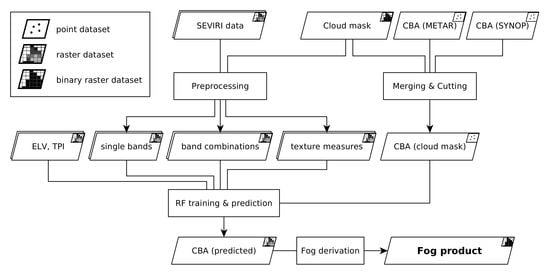
The CBA derivation consists of a hybrid approach (see Figure 2). For each MSG scene, a subset of the SEVIRI data, combinations and geostatistical texture features of the original satellite bands as well as static terrain information are used as input features to train a Random Forest (RF) model. The model is trained towards station report data of CBA values that were contemporaneously reported by METAR and SYNOP stations in Europe. It is then used to predict CBA values for all cloud-covered pixels in the domain. An RF model was chosen as ML approach because RFs are computationally cheap and they follow a relatively simple concept which allows for a straightforward interpretation of the generated model output. It was also shown that for comparable classification algorithms the ML model selection had less impact on the quality of the generated output than the selection of the input variables which is why we decided not to use more complex models cf. [25].
2.2. MSG SEVIRI Data
Meteosat Second Generation (MSG) data from the platforms of Meteosat-8, 9 and 10 were used in this study. These geostationary satellites were located over the South Atlantic at or close to 0.0° E/0.0° N during their operational usage. The on-board Spinning Enhanced Visible and Infrared Imager system (SEVIRI) system scans the full hemisphere every 15 min with a sub-satellite resolution of 3 km in 11 spectral bands and an additional high resolution visible (HRV) channel with a sub-satellite resolution of 1 km. The instrument covers wavelengths from the visible range (0.56 μm) to the thermal infrared (14.40 μm) which allows for a detailed examination of the atmospheric column at these wavelengths [26]. The complete dataset between 2006 and 2015 was acquired from the EUMETSAT in level 1.5 format. These data are geolocated and corrected for all radiometric and geometric effects, which makes them suitable for the derivation of meteorological products [27]. However, it has to be emphasized, that the spatial resolution of the satellite defines the size range of detectable fog patches which impedes the detection of small scale fog occurrences, mainly in complex terrain. Also, the recording frequency of 15 min can leave very short fog events undetected.
In addition to the MSG data, the CMA Cloud mask product (V003) provided by CM-SAF which is mainly based on the MSG SEVIRI data was used to filter the domain for cloud-covered pixels [28].
2.3. METAR Data
Meteorological Aviation Routine Weather Reports (METAR) are standardized weather reports that are reported by airport stations throughout the globe. Their primary use is for aviation safety but they also find application in meteorological tasks. With more than 1300 METAR-reporting stations in Europe, most areas are well covered. Typical report intervals range between 20 min and 60 min which comes close to the temporal resolution of the SEVIRI data. However, measurement instruments and techniques are not internationally standardized which causes variability in the data reliability between METAR stations. Most big airports detect VIS, cloud levels (CL) and CBA using ceilometer and visibility sensors whereas some smaller airfields rely on simple human observation only. As a consequence, from the original data set we filtered land stations with a temporal resolution of less than 30 min and a 24 h report cycle with a complete coverage of the period between 2006 and 2015. After the filtering, 273 stations were left (see Figure 3). It has to be emphasized, that due to the time resolution of 20 min to 30 min, it is possible that very short fog events are not recorded by the stations. However, there is currently no better station network available that provides data on CBA and VIS throughout Europe at comparable frequencies. To get equal temporal resolutions in both data sets, METAR reports of the remaining stations were linearly interpolated onto the 15 min intervals of the MSG data. From this data set, we derived the following information:
Cloud base altitude (CBA): When VIS was reported to be below 1 km, CBA was assumed to be 0 m. When VIS was above 1 km and one or more cloud levels were reported, the altitude of the lowermost level was accepted. In METAR reports, all cloud heights are given in feet above ground level (a.g.l.). In order to obtain CBA values in m a.g.l., CBA values were converted to meters.
Fog (binary): As, by definition, fog occurs when visibility decreases below 1 km, the fog flag was set to true when VIS was reported to be below 1 km at the METAR stations. Otherwise it was set to false. It has to be stated, that sometimes low visibilities can be a consequence of precipitation or high aerosol pollution although in most cases they are caused by fog occurrence in Europe.
2.4. SYNOP Data
One major disadvantage of METAR stations is that they are bound to airport locations. As airports are mostly situated in flat terrain, this means that areas with complex topography and higher elevations are underrepresented in the METAR station data. Although the selected METAR stations cover the spatial extent of the study domain sufficiently, they only reach from −5 m above sea level (a.s.l.) to 793 m a.s.l. elevation. To compensate for this disadvantage, additionally eleven SYNOP reporting stations of the DWD were included in this study that lie in higher terrain (see Figure 3). Their elevations reach from 705 m a.s.l. to 2964 m a.s.l. and thus take better account of the complete altitudinal gradient of Europe. SYNOP data is reported every full hour and the reports contain VIS and CBA observations. Like the METAR reports, this data was preprocessed by temporally interpolating them onto the SEVIRI scan times over Europe. CBA and binary fog information was also extracted in the same way as for the METAR data.
2.5. RF Model Generation
2.5.1. Basic Concept and Implementation
For the prediction of CBA values as part of the fog retrieval, a machine learning model is trained for each scene using pixels with known CBA values (station locations). The model is then used to predict CBA values for all cloud regions within the domain. Here, we use a random forest (RF) regressor, the concept of which was first introduced by Breiman [29]. An RF regressor is an ensemble learning method that is based on a large number of decision trees. Each tree is trained separately by taking a bootstrap sample from the training data set. It is built such that at each node of the tree, a random subset of the original input features is used to split the node. Each node is split by minimizing an error function for the subsets of the respective node. This procedure is recursively repeated until the complete training data set is covered. The RF regression method was chosen because it runs efficiently on large data sets and it can easily handle vast numbers of input features. As the procedure provides internal estimates of the different feature importances it is also well suited to help filtering for those features that are relevant for the prediction of the target feature. The RF model procedure was implemented in Python using the Scikit-learn package that is provided by Pedregosa et al. [30].
2.5.2. Preprocessing and Input Features
In previous studies, fog occurrence was mainly linked to atmospheric conditions that favored radiative fog formation which is why FLS is identified in a first step towards fog identification in these studies (see Cermak and Bendix [22]). However, a preliminary investigation of the ground truth and satellite data sets used in this study showed that only 33.2% of all fog occurrences reported by the ground truth stations could actually be identified as covered by FLS from the satellite’s perspective. There are three reasons for this: (1) Multiple cloud layers obscure the satellite’s view: 60.1% of all pixels for which FLS was reported by the respective ground truth station were covered by higher opaque clouds which prevents proper FLS detection from space; (2) Fog patches smaller than 9 km2 are too small for the MSG resolution and cannot be captured by the satellite accordingly: 23.2% of all pixels with fog occurrence reported by the respective ground truth stations could not be identified as cloudy by the satellite; (3) Orographic fogs and other fog types that are not dependent on local radiative cooling are not dependent on FLS occurrence and can form below other cloud types. Due to these reasons, a meaningful fog climatology can only be generated by considering all cloud-covered pixels. Contrary to previous approaches, a preliminary filtering of FLS pixels was thus not conducted in this study.
A tuning data set was extracted from the original data so that the RF models could be tweaked in order to deliver the best possible results: In a first step, reflectances as well as brightness temperatures of each single band were extracted from the raw data. After that the SEVIRI and METAR/SYNOP data sets were merged by assigning each CBA report from each METAR/SYNOP station to the corresponding pixel values of each band of the respective SEVIRI scene. This was done for all 342’328 available SEVIRI scenes between 2006 and 2015. As we were only interested in regions that are covered by clouds, the merged data set was reduced to samples where the CM-SAF cloud mask product [28] showed cloud-covered pixels. From this global data set a sample data set was extracted by selecting 100 random scenes from each single month which resulted in a data set of 11’993 valid MSG scenes with their corresponding METAR/SYNOP reports which again yielded in 395’560 samples in the final tuning data set.
As the combination of different bands proved to be helpful to detect FLS e.g., [16], it seemed reasonable to also provide the models with band combinations. Although this leads to partial redundancy in the input features, it helps to highlight otherwise unapparent patterns in the data. Cloud top height (CTH), liquid water path (LWP) and cloud phase (CP) can be used as proxies towards CBA estimation. As these microphysical properties can be derived from band combinations between the water vapour bands and the middle and thermal infrared bands, the five most important combinations between these bands were included in the model data (cf. Kühnlein et al. [31], Thies et al. [32]).
Still, spatial information, such as the heterogeneity within cloud patches, is not covered by only looking at single pixel values. Information about spatial variance within a given raster data set, however, can improve the output of ML approaches. This is exploited in many ecological studies, e.g., Wijaya et al. [33] or Schulz et al. [34]. As spatial information in the form of standard deviations within cloud patches is also included in the FLS detection algorithms of Cermak and Bendix [18] and Egli et al. [20], it seemed promising to also provide this information to an ML model to improve the prediction of CBA values. Thus, several geostatistical texture features of the 5 × 5 pixel surroundings of each METAR station were provided for the model training. These measures include standard deviations (STD), variograms (VAR), madograms (MAD) and rodograms (ROD) of each band and cross variograms (CV) as well as pseudo cross variograms (PCV) of each band combination. Please refer to Equations (A1)–(A5) in the Appendix A for a detailed mathematical description of the listed features.
Although MSG SEVIRI level 1.5 data includes basic corrections, two effects caused by the satellite’s geostationary orbit have to be considered: Variations in the solar position and in the satellite viewing angle (SVA).
Seasonal and diurnal variations in the solar cycle influence the responses of the MSG bands, especially those in the visible and near infrared range between 0.6 μm and 3.9 μm. However, these variations have to be considered in the model training only if the model should be able to predict CBA values for multiple time steps with changing solar positions. In our approach, however, an independent RF model is trained separately for each scene. As intra-scene solar angle variations are relatively small due to the small domain size, the sun’s position was not considered as an input feature to the model training.
SVA reflects the distance between the earth’s surface and the satellite sensor. This also means that the atmospheric column and therefore the amount of absorbing gases increase with growing SVA. This causes distortions in the value distributions of the channels within the domain. Unfortunately, SVA cannot be used as an input feature for the RF training in order to correct this effect, because its high spatial autocorrelation would lead to artifacts in the model prediction results around the station pixels. Instead, the scenes were cleared from the influence of the SVA before handing them over to the RF training. An empirical approach was chosen: First, average reflectance and brightness temperature values were calculated from all 11’993 scenes of the tuning data set separately for each band. Then, regressions were calculated between the averaged bands and the corresponding SVA values. This was done separately for each band. The regression coefficients determined in this way were then applied to each scene using Equation (A7) to remove the SVA influence from the data before handing them over to the RF training. An example of the SVA correction is depicted in Figure 4.
As CBA is substantially defined by the condensation level which is closely linked to the planetary boundary layer along warm fronts which again is closely linked to the underlying topography, terrain elevation (ELV) as well as the Topographic Position Index (TPI) were also added to the training data. TPI values are highly dependent on the window size used for their calculation. Thus, the correlation coefficients of a linear correlation between CBA and TPI were calculated for different window sizes using the tuning data set (see Figure 5). A window size of 25 pixels edge length was used for the final RF models since window sizes with an edge length of 25 pixels resulted in a maximum value of 0.22.
ELV was extracted from the WorldClim DEM generated by Hijmans et al. [35]. Please find a detailed description of the calculation of the TPI in Equation (A6) in the Appendix A. All input features that were used during the RF model generation are listed in Table 1.
2.5.3. Feature Selection
In order to reduce the “curse of dimensionality” [36] and to obtain the largest possible information content from the original data while reducing noise artifacts due to irrelevant information, the features that are most relevant for CBA derivation were extracted from the original data set. To this end, a recursive feature elimination (RFE) was conducted for each scene of the tuning data set starting from randomly varying 20 feature subsets. In each step of this iterative procedure the original number of input features was reduced by one element and the model quality was calculated using an out-of-bag (OOB) score. The OOB score is calculated on the basis of the left-out data during model fitting and is similar to the outcome of a cross-validation [37]. This iterative procedure was repeated for each scene until only one feature remained. The results are depicted in Figure 6.
Average RF model performances were almost constant with scores around 0.10 for feature counts from 74 down to 14. On average, the best model performance with an of 0.11 was reached at 14 remaining features in the tuning data set. Removing further features from the set resulted in worse scores. Thus, for the final RF model fitting procedures, the 14 features with the highest average rankings were filtered from the original set of 74 features and used as training input for the final RF models (see Figure 7).
The plot shows that the terrain features were identified as having the highest explanatory power in terms of CBA derivation. This shows that the models identified the close link between condensation level—which defines the lower cloud boundary—and terrain elevation. The high ranking of TPI can probably be attributed to the fact that TPI can help identifying situations where the condensation level does not closely follow the terrain elevation but is shifted towards or away from the surface due to local ridges and troughs. However, the standard deviations of these two features are relatively high compared to the other features. This is probably due to the fact that TPI and ELV only provide explanations for the cloud height in LS situations where only the higher elevations reach into the cloud layer. This distinction is not necessary for plane-filling fog fields and the two terrain features cannot contribute to the CBA retrieval in these cases.
The bands in the thermal infrared, especially at 3.9 μm and 10.8 μm make up the biggest part of the remaining features. This is not surprising as the thermal radiance emitted by the surface and by clouds which is recorded by these bands can be used as a proxy for cloud top altitudes. This is also the reason why these bands are vastly used in many cloud altitude derivation algorithms [38]. Additionally, due to the different emissive behaviors of small cloud droplets in the 3.9 μm and 10.8 μm bands, the differentiation between high and low lying stratus layers is possible which can be used as a first proxy towards the final CBA estimation. As the T 3.9–10.8 combination is placed on rank 4 it seems that the models were indeed able to use this information for the CBA prediction.
The water vapour bands at 6.2 μm and 7.3 μm do also make a major contribution to the CBA estimation. This is surprising in that both bands are insensitive to the lower atmosphere due to the strong water vapor absorption in the upper layers. The bands are thus not able to capture ground-level atmospheric conditions which are expected to be most relevant for the derivation of low cloud base altitudes. As the bands are, however, able to detect upper atmospheric circulation patterns, they can bring information about the large-scale synoptic situation into the model which could indeed help to deduce low cloud altitudes. Due to their ability to derive humidity information from the middle and high troposphere, both bands can also be used in combination with the IR window bands to differentiate between convective and stratiform clouds [39]. This information is crucial for the final fog retrieval as low visibility due to fog is more likely to happen below a stratiform cloud layer than below convective systems (e.g., as a result of ground touching LS in anticyclonic conditions or as frontal fog along warm fronts in winter) .
On the other hand, the visible bands at 0.6 μm and at 0.8 μm ranked lowest on the feature list and were not included in the final model training. This was expected as they only capture the reflectance of sunlight and no thermal radiance emittance. Though this helps to delineate cloud entities during daytime, it does not provide information about their altitude via brightness temperature estimations.
In general, the models chose to use band combinations and texture measures over the use of single bands. It is also obvious that the models preferred to use two bands in combination as the only texture measure that was used is the pseudo cross variogram. All this suggests that the prior processing of the raw data was indeed helpful in uncovering otherwise obfuscated patterns.
2.5.4. Parameter Tuning
Following the approach of Kuhn and Johnson [40], the total number of decision trees () and the number of input features used at each node () were tuned to get optimal settings for the RF model. This was done in an iterative procedure with ranging from 50 to 300 and ranging from 1 to 5. For each parameter set RF models were fitted to the tuning data set and the OOB score was calculated. The parameter tuning procedure was run on an Intel Core i7-5600U CPU @ . The results are shown in Figure 8.
The model performance strongly increased in the beginning and then slowly approached an upper limit of about 0.11 after . With the score values were significantly lower than when more features were considered at the nodes. On the other hand, values larger than 3 didn’t increase the prediction performance. With values growing above 250 the performance increase began to stagnate whereas processing times linearly grew further (see Figure 8b). As a compromise between prediction accuracy and processing time, a cut has been made at and was set to 3 in the final RF models that were used for the fog retrieval scheme.
2.5.5. Application of the RF Models and Fog Derivation
Feature elimination and parameter tuning procedures were carried out using the tuning data set to determine both the final input feature set and the best model parameters. These settings were than applied to the processing scheme of each single MSG scene. Ground truth station observations of CBA that were temporally interpolated onto the MSG scan times were merged with the satellite information and used as model input (see Figure 9a for an example). Within the scope of this study, only the SYNOP stations in Germany were available as representatives for higher terrain and exposed locations. As these locations showed significantly lower CBA values than the remaining stations and due to the spatial autocorrelation in the input features, a simple application of the RF models including all input features would have led to an adequate prediction of CBA values within Germany but a strong overestimation of CBA values in the rest of the domain. Therefore, the RF application had to be divided into two steps for each scene. First, a model was trained using all available METAR stations within the respective scene that were covered by clouds. As input feature set only the satellite bands and their derivations (geostatistical texture features as well as band differences) were used. The CBA values predicted with this model are therefore based only on the information content of the satellite bands. A second model was then trained using the output of the first model and TPI as well as ELV as input features. Using this two-step approach, the influence of the terrain could be incorporated into the model predictions without spatially over-fitting CBA values to Germany.
Because of their structure, RF models are able to predict almost perfectly the target variables of samples that appear in both, the training data set as well as in the prediction data set. The resulting overfit of the model to the station locations can be prevented by a slight change in one of the independent variables of the sample which is why for each model training procedure, instead of taking the actual pixel values of the station locations, the average of their direct pixel neighbours were used. Although the data accuracy is artificially impaired by this step, it is necessary to prevent the algorithm from overfitting to the station pixels. Figure 9b shows an example output of the RF model predictions for 15 November 2011 00:00 UTC. The model was clearly able to distinguish high clouds over southwest France, Spain and the Balkans from fog and LST patches in England, Germany, northern Italy and the Benelux countries.
As, by definition, fog occurs where a cloud touches the ground, pixels with values equal to or below zero could theoretically be classified as pixels with fog occurrence. However, reported CBA values are never negative and thus the RF model predictions are never smaller than zero although the theoretical condensation level could actually be considerably lower than the terrain elevation. As only the pixels of fog reporting stations can have CBA values of zero, this would lead to a strong underestimation of fog occurrence for non-station pixels without an application of a threshold to the CBA predictions. The threshold values were derived by gradually lowering the layer of predicted CBA values and calculating Heidke Skill Scores (HSS, see Equation (A12)) of derived fog occurrences (CBA ≤ 0 m) and observed fog occurrences (VIS ≤ 1000 m) for each step. The shift resulting in the highest HSS was accepted as threshold for the final fog derivation. The thresholds fluctuated around a median of 70 m and remained below 247 m in 90 percent of the cases. The resulting output of this step is shown in Figure 9c together with fog observations of the ground truth stations. By applying the threshold value to the CBA predictions, the fog retrieval scheme provides a reasonable fog distribution for the study domain. The Po valley and large parts of southern Germany and northeastern France were marked as fog-covered. In particular, small-scale areas such as the Upper Rhine Valley were recognized as fog-free (elevated LST), while the slopes of the nearby Black Forest are suspected to be covered in fog. However, large-scale structures that can be anticipated from the station data are also visible in the product: While the southern edge of the FLS patch, which stretches from the Netherlands through northern Germany to Poland, was identified as ground-touching, the northern areas within this patch are marked as fog-free. This is consistent with the station reports which indicate that the condensation level only reaches the surface at the southern end of the patch.
3. Validation
To get an overview of the reliability of the fog retrieval scheme and the validity of the produced data set, an extensive validation procedure was conducted. Here we chose to validate the derived CBA data and the final fog product using the METAR/SYNOP stations that were also taken for the RF training in a cross validation approach.
At this point it has to be stated, that satellite products are not directly comparable to ground truth data for a number of reasons: Instabilities in the satellite’s orbit cause parallax shifts which lead to ambiguities in the assignment of ground-truth data locations to pixel coordinates. Also, different temporal resolutions in both datasets result in timing uncertainties and multiple cloud layers as well as subpixel effects resulting from the satellite resolution at margins of fog patches additionally impede the comparison between satellite and ground truth data. All these insufficiencies cause ambiguities in the comparison process. However, there are no other reliable data sources for fog occurrence that provide better information on fog distribution on a continental scale.
The validation was conducted using a leave-location-out (LLO) cross validation procedure. By using an LLO approach, it is guaranteed that the validation results are not corrupted by a possible overfit of the model outputs to the station pixels and that the validation results are generally applicable to the complete study domain. The LLO procedure was carried out in such a way that the RF models were trained for each scene of the tuning data set using the input data of all but one station. The CBA prediction results were then compared to the observations of the left-out station. Fog was derived from CBA values by application of the threshold technique explained in Section 2.5.5. As the LLO cross validation procedure is very time-consuming and computationally expensive, only 10 randomly drawn stations per scene were used for the fog derivation. Observed and predicted CBA and GF values were then compared between these stations. This procedure was repeated for all scenes in the tuning data set. As the models were only trained for cloud covered regions in the CM-SAF cloud mask, only these pixels were included in the validation procedure. This resulted in a total of 118’145 samples, which were included in the validation procedure. Based on the generated data set, the following validation measures were calculated to get an overview of the quality of the product.
Average absolute differences between predicted and observed CBA values were calculated for each sample and MAE (Mean Absolute Error) values were computed for each station. PC (Percentage Correct), POD (Probability Of Detection), FAR (False Alarm Ratio) and HSS (Heidke Skill Score) were calculated for the fog predictions accordingly. Please refer to Equations (A8)–(A12) in the Appendix A for a detailed description of these validation measures. While PC, POD and FAR address very specific features of the fog data set only, the HSS compares the forecast accuracy of the product to the forecast accuracy of a random guess procedure. This gives an overall indication of the validity of the algorithm output, independent of the fog frequency. The HSS ranges between −1 and 1. Negative values indicate that the model output is worse than a random guess, a value of zero means no skill increase compared to a random guess while a perfect prediction obtains a HSS of 1. All verification measures were calculated for all cloud covered samples in the tuning data set. Diurnal and annual variations in the verification measures are plotted in Figure 10 and Figure 11.
MAE values fluctuate around an average of 298 m with minima of 251 m at 08:00 UTC and 267 m in February and maxima of 340 m at 23:00 UTC and 325 m in July (see Figure 10 and Figure 11a). The probable explanation for the better performance in winter is that LST layers are more dominant in winter than in summer. Therefore, the heterogeneity within the clouds is smaller in winter which in turn simplifies the derivation of cloud base altitudes.
As already mentioned in the introduction, the validation data set also shows that fog frequency is considerably higher at night and in winter due to the general decrease of the condensation level than during the day and in the summer months. Daily and annual frequency variations are stronger in the predicted values than in the observation data. Higher amplitudes in winter and at night in the predictions most likely are a consequence of fog occurrences in the lowlands are more dominant in these times. It is more difficult for the retrieval scheme to correctly derive the spatial extent of these fogs, since they occur in flat terrain and vertical shifts of the thresholds used for fog derivation have a stronger effect here. This leads to a slight overestimation in the generated product during these times. The daily maximum is reached around 04:00 UTC with 8.3% in the observations and 9.5% in the predictions. Fog frequency then decreases steadily as the day progresses and reaches its minimum of 2.4% in the observations and 2.1% in the predictions at 15:00 UTC. Afterwards it starts to rise again steadily. The annual curve behaves similarly with a maximum of 8.5% in December (observations) and 11.1% in January (predictions). Minima occur in June with 2.8% (observations) and 2.1% (predictions). With an average value of 95.6%, PC is always on a high level. However, with maxima of 98.1% at 15:00 UTC and 97.5% in June as well as minima of 93.2% at 03:00 UTC and 92.7% in January, the PC curve is almost an inversion of the fog frequency curve in both, diurnal and annual averages. This is due to the fact that significantly fewer fog events have to be "hit" during the day and in the summer months which drives up the PC due to the large number of true negatives (see Figure 10 and Figure 11b).
The shape of the POD curve shows that the probability of correctly predicting a fog event is higher in winter with a maximum of 0.74 in December, despite the high PC values in summer. Contrary, in summer POD generally decreases down to a minimum of 0.44 in June. The poor performance of the POD in summer is mainly due to the fact that the absolute number of fog events is very low in the warm months which makes a “hit” more difficult. The FAR values behave similarly to the POD values at a lower average level of around 0.41. They also show a less pronounced daily and annual amplitude with maxima of 0.48 at 11:00 UTC and 0.49 in June as well as minima of 0.34 at 20:00 UTC and 0.35 in August. This means that the relative rate of false positive predictions stays on a moderate level for each period. Both, diurnal and annual HSS curves show very little variation. With an average of 0.58 the scores consistently remain on a high level and thus indicate the good performance of the scheme throughout the complete time period (see Figure 10 and Figure 11c).
In addition to the direct validation procedure on a 15 min level we compared average fog frequencies of the product to average station observations of the complete time period from 2006 to 2015 (see Figure 12). We can see that the product matches the observations with a bias of −0.2% and an absolute average error of 0.7% very well at the METAR stations. At the SYNOP station pixels, however, the bias is much stronger with −10.4% which leads to an underestimation of fog frequencies in mountainous regions. This is mainly due to the fact that the scheme can only flag a pixel as covered by fog if the satellite was able to identify it as cloudy beforehand. All fog patches with sizes in the subpixel range thus cannot be detected by the approach and are therefore not included in the statistics. This effect is stronger at SYNOP stations because the probability of subpixel fog patches is higher in the heterogeneous terrain of the SYNOP stations due to the large differences in terrain height within small distances. Nevertheless, with an average absolute error of 1.1% over all stations, we can assume that Figure 13 gives a reasonable overview of the general distribution of the fog frequency in Europe.
To compare the performance of our approach with the performance of existing physics-based methods, the same verification measures were calculated from the confusion matrix of SOFOS (Satellite-based Operational Fog Observation Scheme) presented in Cermak and Bendix [22]. The results are listed in Table 2 together with the verification measures of this study. While SOFOS was able to reach a higher PC value (0.99 vs. 0.95), the hybrid scheme performed better in the other verification measures. The high PC score in SOFOS results from a large number of correctly predicted non-fog situations which is associated with generally low fog frequencies in the investigated time period. With POD values of 0.61, however, the hybrid scheme was able to correctly detect fog occurrences with a higher precision than SOFOS (0.52) while fog-free situations were less often misclassified as foggy with FAR values of 0.41 for the hybrid scheme and 0.66 for SOFOS. Overall, this results in a better performance of the hybrid approach with an HSS of 0.58 compared to 0.41 for SOFOS. It has to be emphasized, however, that the results of both schemes cannot be directly compared to each other as both were evaluated for different time periods. Also, SOFOS is designed for radiation fog conditions at sun elevations above 10° whereas the hybrid approach is generally applicable for all sun elevations and fog types.
In summary, it can be said that the scheme was able to detect fog with higher precision than previous physics-based approaches despite the problems that the satellite-based hybrid approach has to deal with and although RF model scores of 0.11 were relatively low. With slight variations in the daily and yearly cycle, the validation measures consistently indicate satisfactory data quality in the final fog product.
4. Fog Climatology
The fog retrieval scheme was applied to each of the 342’328 available SEVIRI scenes from the period between 2006 and 2015. The resulting fog product was averaged over all scenes (see Figure 13). It is clearly visible that the fog frequency distribution is highly dependent on the terrain and that there can be strong changes in the fog frequency within a few kilometers, especially in and around mountain ranges. Lowlands and coastal regions show low fog frequencies between 0% and 5%, while mountainous regions with a maximum of 39% in the Central Alps are dominated by much higher fog frequencies.
At this point it has to be emphasized that any kind of ground touching cloud is interpreted as a fog event by the algorithm. The map thus does not only indicate radiation fog frequencies that are associated to FLS patches but all kinds of fog types. Also, since fog only prevails where an FLS patch actually touches the ground and since CBAs are relatively homogeneous within an FLS patch, fog usually only occurs at the margins of FLS patches where the terrain height increases. The fog map is therefore almost an inverted version of the FLS map that was presented in Egli et al. [20] where lowlands and river valleys are prone to higher FLS frequencies than their neighbouring mountain ranges.
Another peculiarity is that the fog map reveals the main flow direction of low and humid/saturated air masses in mountain ranges. Orographic fog forms as a result of condensation due to uplift of humid air at windward mountain slopes. Cloud fog results from stratiform clouds that are formed and transported along warm fronts towards the mountain range. Both fog types form at the windward side of the mountain ranges whereas the leeward side is fog free. This causes higher fog frequencies at the side of the main wind direction. In the Cantabrian Mountains, the Pyrenees, the Alps and the Scandinavian mountains this results in higher fog frequencies on the north and west slopes of the mountain ranges.
In order to investigate the spatial differences in the diurnal and annual variations in fog frequency, anomalies were computed for individual hours and seasons (see Figure 14 and Figure 15). The anomaly values were calculated as the differences between each hourly and each seasonal 10-year average and the global mean from Figure 13. Values are given in percentage points (pp)—the arithmetic difference of two percentages.
Figure 14a–d give a good overview of the daily fluctuations in fog frequency. During the first half of the night there is a slightly higher fog frequency than on average in lower altitudes but a strong negative anomaly above 900 m. The distribution pattern changes during the night so that in the morning hours around 06:00 UTC high fog frequencies are visible at all elevation levels. This is due to the fact that the conditions for radiation fog, which forms in lowlands and valleys during anti-cyclonic weather situations, generally improve over night. Additionally, the condensation level decreases as a result of the general drop in temperature until sunrise, which means that the mountain slopes and higher mountainous regions are also covered in fog more frequently as a result of cloud base lowering fog.
After sunrise the situation changes drastically. Lowlands below 1000 m show a negative anomaly at 12:00 UTC whereas the higher regions, especially the Alps and the Pyrenees are covered in fog far more frequently now. However, low visibility situations are not a result of radiative cooling in these cases, but more likely due to orographic fog formation. This happens when humid air is lifted upwards at the windward side of the mountain ranges during cyclonic weather conditions which leads to condensation due to adiabatic cooling. At 18:00 UTC the fog frequency is at a low in both the higher regions and the lowlands. Frequencies increase only slowly as the night progresses, starting in the lowland.
As expected, the maps of the seasonal anomalies (Figure 15a–d) show that fog frequencies increase in autumn and especially in winter. On the other hand, in spring and even more so in summer, there is a substantial decrease in the general fog frequency. Terrain elevations around 1500 m show strongest variations whereas the lowlands below 500 m and mountainous regions above 2500 m are characterized by much less seasonal variation (Figure 15e–h).
In winter, the strongest positive anomalies occur in the uplands and at the slopes of high mountain ranges. This applies to the Cantabrian mountains, the Pyrenees and the Sierra Nevada in Spain, the Cévennes, the Vosges and the Jura in France, the Scandinavian mountains, the Highlands in Scotland, the Black Forest, the Swabian Alb, the Harz Mountains, the Rhön, the Ore Mountains and the Bavarian Forest in Germany, the High Tatras, the Carpathians, the Dinaric mountains in Eastern Europe, the Apennines in Italy and the Alps. The reason for this is the general presence of more FLS and the lowering of the condensation level during winter. As a result, mountain slopes and areas of relative elevation often protrude into the extensive stratus fields in the lowlands. Fog frequencies in the lowlands are also increasing in winter. Since the condensation level does not reach the ground level of the lowlands in most of the cases, the difference to the long-term mean is, however, smaller here. Then again, some lowland regions show vastly more fog occurrence in winter. The northern and southern flanks of the Po valley are such an exception. With positive anomalies of up to 9.1 pp fog is much more prominent in these regions. The Po valley has long been known for the frequent occurrence of fog and has therefore already been the subject of several fog research projects (see Bendix [41], Fuzzi et al. [42], Mariani et al. [43], Wendisch et al. [44]). Due to the orography of the valley, which is enclosed by the Alps and the Apennines on three sides, strong temperature inversions can develop here during anticyclonic conditions. These temperature inversions promote the development of large fog patches within the whole valley. Another peculiarity of winter fog distribution is that the only negative anomaly can be found in the very high-altitude areas above 2200 m a.s.l. in the Alps and in the Pyrenees. This is probably due to the fact that these regions often rise above the FLS layers that are capped by the temperature inversion.
In spring, the fog anomaly in the lowlands shifts into the negative and in the higher regions above 900 m a.s.l. into the positive. This trend can be observed more strongly in the North than in the South, where also in spring higher values are reached than in the long-term average. The reason for this is the increasing condensation level while LST is still abundant. As a result, lowlands and lower mountain ranges are often below the condensation level, while the high mountain regions are covered in ground touching clouds more often.
This trend comes to an extreme during summer. Now, there is a strong overall negative fog anomaly and the areas that showed significantly more fog in winter show much less fog than in the long-term average. Even the high mountainous regions above 2000 m show a slight negative anomaly. High summer temperatures prevent the formation of deep lying stratus fields during anticyclonic conditions. As a result, neither the lowlands nor the slopes of the mountain ranges are covered in fog during these conditions. Even the highest regions are more frequently fog-free as only the fast moving clouds during cyclonic conditions are causing temporal low visibility situations here.
This trend is reversed again during autumn due to the general decrease of the condensation level. The lowlands start to be covered with fog more often again, while areas above 1300 m show a negative anomaly.
In summary, it can be concluded that the hourly and seasonal fluctuations in the spatial distribution of fog frequencies are adequately reflected by the product.
5. Conclusions
The hybrid fog retrieval approach presented in this paper is able to derive spatially explicit and temporally highly resoluted fog distribution data for Europe. Due to the incorporation of satellite and ground truth station data as well as additional terrain information it is able to capture the strong spatiotemporal dynamics of fog formation and dissipation sufficiently. The results of an extensive cross-validation procedure show that the generated fog product is capable of reflecting the diurnal and annual fluctuations in fog frequency very well.
The generated 10 year baseline fog climatology is the first of its kind. It provides valuable information on the fog frequency distribution over land on a 15 min interval and it reveals even small scale spatial patterns. The product shows that fog occurrence is highly dependent on the topography. High mountain ranges and uplands with a distinct relative elevation in comparison to their surroundings are characterized by high fog frequencies whereas lowlands and coast regions have much lower fog frequencies. During winter and night the strongest positive anomalies occur while in summer and during daytime the fog frequencies are much lower on average.
The product also shows, that amplitude and temporal lag of the fog frequency variation change with terrain elevation which can be attributed to the formation of different fog types. Similar results are found in recent studies in which radiation fog is associated with cold anticyclonic conditions in the lowlands and advection or cloud base lowering fog is linked with warm cyclonic conditions in elevated terrain [45,46,47].
In order to develop a deeper understanding of the processes of fog dynamics, it is planned to investigate the fog product for different synoptic large-scale weather conditions and to determine allochthonous and autochthonous influence factors of fog formation and dissipation. Since both, METAR and SYNOP measurements, are available in quasi real-time, the developed algorithm can be used operationally in the future to continuously advance the product.
The product quality will be further improved by including additional station observations in different terrain types as well as more elevation levels and by using pan-sharpening methods based on the HRV band in upcoming scheme adaptations. The algorithm can also be transferred without any major adjustments to the upcoming third generation of the Meteosat satellite series which will provide higher spatial, temporal and spectral resolutions. This should result in further improvements of the product accuracy.
Monthly averages of the complete fog product data set are freely available for download at dx.doi.org/10.5678/LCRS/DAT.311.
Acknowledgments
This study was performed within the project “Ground fog detection and analysis with Machine Learning” (GFog-ML), generously funded by the German Research Foundation (DFG projects: BE1780/40-1 and TH1531/4-1). It is also part of the Satellite-based evaluation of weather conditioned LiDAR measurement downtimes project (LiMeS), generously funded by the Bundesministerium für Wirtschaft und Energie (BMWI project: 0324159D). The authors also thank EUMETSAT for providing the MSG satellite data used in this study and the DWD for providing the SYNOP station data.
Author Contributions
S.E., B.T. and J.B. conceived and designed the experiments; S.E. performed the experiments; S.E. and B.T. analyzed the data; B.T. and J.B. contributed materials/analysis tools; S.E. wrote the paper.
Conflicts of Interest
The authors declare no conflict of interest. The founding sponsors had no role in the design of the study; in the collection, analyses, or interpretation of data; in the writing of the manuscript, and in the decision to publish the results.
Abbreviations
The following abbreviations are used in this manuscript:
| CBA | Cloud Base Altitude |
| CL | Cloud Levels |
| CM-SAF | Satellite Application Facility on Climate Monitoring |
| CP | Cloud Phase |
| CTH | Cloud Top Height |
| CV | Cross Variogram |
| DEM | Digital Elevation Model |
| DWD | German Weather Service |
| ELV | Terrain Elevation |
| FAR | False Alarm Rate |
| FLS | Fog and Low Stratus |
| HRV | High Resolution Visible band |
| HSS | Heidke Skill Score |
| LLO | Leave Location Out |
| LST | Low Stratus |
| LWP | Liquid Water Path |
| MAD | Madogram |
| MAE | Mean Absolute Error |
| METAR | Meteorological Aviation Routine Weather Reports |
| ML | Machine Learning |
| MSG | Meteosat Second Generation |
| OOB | Out Of Bag |
| PC | Percentage Correct |
| PCV | Pseudo Cross Variogram |
| POD | Probability Of Detection |
| RF | Random Forest |
| ROD | Rodogram |
| SEVIRI | Spinning Enhanced Visible and Infrared Imager |
| STD | Standard Deviation |
| SVA | Satellite Viewing Angle |
| SYNOP | Synoptic Weather Observations |
| TPI | Topographic Position Index |
| VAR | Variogram |
| VIS | Horizontal Visibility |
| WMO | World Meteorological Organization |
Appendix A
The following geostatistical texture features were used in this study. All features were calculated for 5×5 pixel surroundings with a lag distance of 1. The Variogram provides information about the correlation of the data with distance. It is defined as
A slight variation to the Variogram is the Madogram which takes the absolute values of the differences:
The Rodogram takes the square root of all differences:
The Cross Variogram takes information from two different data inputs to account for cross correlation between two bands:
The Pseudo Cross Variogram calculates the differences of cross pairs between two data inputs directly:
For all geostatistical texture features is the number of pairs for lag distance h. and are the coordinates of pixel pairs that are separated by lag distance h for each pair i. v and w are the values of the pixels of different raster inputs at locations and [33].
The Topographic Position Index gives information about the relative elevation of a pixel in comparison to its neighbouring pixels. Positive values indicate a peak or a ridge, negative values indicate a valley. It is calculated with the following formula:
where is the index of the center pixel and is the index of a neighbour pixel. v is the value of a pixel at a given index and n is the number of neighbouring pixels that are included in the calculation [48].
Distortions in the MSG bands due to the Satellite Viewing Angle were corrected for using the following formula:
where is the value of pixel i of the corrected band, is the value of the corresponding pixel of the original band, is the average of all pixel values of the original band, is the SVA value of the corresponding pixel, s is the slope and t is the intercept of the linear regression that was determined before.
CBA prediction accuracy was evaluated using the Mean Absolute Error:
where n is the number of predictions, is the predicted and is the observed value.
For the assessment of the confusion matrices that were produced in the comparison procedure of predicted and observed fog occurrences, the following verification measures were calculated:
where a is the sum of all correctly predicted fog occurrences (True Positives) and b is the sum of all incorrectly predicted fog occurrences (False Positives). c is the sum of all False Negatives and d is the sum of all True Negatives accordingly.
References
- Bendix, J.; Eugster, W.; Klemm, O. Fog—Boon or bane? Erdkunde 2011, 65, 229–232. [Google Scholar] [CrossRef]
- Nemery, B.; Hoet, P.H.M.; Nemmar, A. The Meuse Valley fog of 1930: An air pollution disaster. Lancet 2001, 357, 704–708. [Google Scholar] [CrossRef]
- Köhler, C.; Steiner, A.; Saint-Drenan, Y.M.; Ernst, D.; Bergmann-Dick, A.; Zirkelbach, M.; Ben Bouallègue, Z.; Metzinger, I.; Ritter, B. Critical weather situations for renewable energies—Part B: Low stratus risk for solar power. Renew. Energy 2017, 101, 794–803. [Google Scholar] [CrossRef]
- Gultepe, I.; Tardif, R.; Michaelides, S.C.; Cermak, J.; Bott, A.; Bendix, J.; Müller, M.D.; Pagowski, M.; Hansen, B.; Ellrod, G.; et al. Fog Research: A Review of Past Achievements and Future Perspectives. Pure Appl. Geophys. 2007, 164, 1121–1159. [Google Scholar] [CrossRef]
- Henschel, J.R.; Seely, M.K. Ecophysiology of atmospheric moisture in the Namib Desert. Atmos. Res. 2008, 87, 362–368. [Google Scholar] [CrossRef]
- Johnstone, J.A.; Dawson, T.E. Climatic context and ecological implications of summer fog decline in the coast redwood region. Proc. Natl. Acad. Sci. USA 2010, 107, 4533–4538. [Google Scholar] [CrossRef] [PubMed]
- Lehnert, L.W.; Thies, B.; Trachte, K.; Achilles, S.; Osses, P.; Baumann, K.; Schmidt, J.; Samolov, E.; Jung, P.; Leinweber, P.; et al. A Case Study on Fog/Low Stratus Occurrence at Las Lomitas, Atacama Desert (Chile) as a Water Source for Biological Soil Crusts. Aerosol Air Qual. Res. 2018, 18, 254–269. [Google Scholar] [CrossRef]
- Pinto, R.; Larrain, H.; Cereceda, P.; Lázaro, P.; Osses, P.; Schemenauer, R. Monitoring fog-vegetation communities at a fog-site in Alto Patache, South of Iquique, Northern Chile, during “El Niño” and “La Niña” events (1997–2000). In Proceedings of the Second International Conference on Fog and Fog Collection, St John’s, NL, Canada, 15–20 July 2001; International Development Research Center: Ottawa, ON, Canada, 2001; pp. 293–296. [Google Scholar]
- Vautard, R.; Yiou, P.; van Oldenborgh, G.J. Decline of fog, mist and haze in Europe over the past 30 years. Nat. Geosci. 2009, 2, 115–119. [Google Scholar] [CrossRef]
- Bendix, J. A satellite-based climatology of fog and low-level stratus in Germany and adjacent areas. Atmos. Res. 2002, 64, 3–18. [Google Scholar] [CrossRef]
- Duda, D.P.; Stephens, G.L.; Stevens, B.; Cotton, W.R. Effects of Aerosol and Horizontal Inhomogeneity on the Broadband Albedo of Marine Stratus: Numerical Simulations. J. Atmos. Sci. 1996, 53, 3757–3769. [Google Scholar] [CrossRef]
- García-García, F.; Zarraluqui, V. A fog climatology for Mexico. Erde 2008, 139, 45–60. [Google Scholar]
- Scherrer, S.C.; Appenzeller, C. Fog and low stratus over the Swiss Plateau—A climatological study. Int. J. Climatol. 2014, 34, 678–686. [Google Scholar] [CrossRef]
- Tardif, R.; Rasmussen, R.M. Event-Based Climatology and Typology of Fog in the New York City Region. J. Appl. Meteorol. Climatol. 2007, 46, 1141–1168. [Google Scholar] [CrossRef]
- Avotniece, Z.; Klavins, M.; Lizuma, L. Fog climatology in Latvia. Theor. Appl. Climatol. 2015, 122, 97–109. [Google Scholar] [CrossRef]
- Bendix, J.; Bachmann, M. Ein operationell einsetzbares Verfahren zur Nebelerkennung auf der Basis von AVHRR-Daten der NOAA-Satelliten. Meteorol. Rundsch. 1991, 43, 169–178. [Google Scholar]
- Musial, J.; Hüsler, F.; Sütterlin, M.; Neuhaus, C.; Wunderle, S. Daytime Low Stratiform Cloud Detection on AVHRR Imagery. Remote Sens. 2014, 6, 5124–5150. [Google Scholar] [CrossRef] [Green Version]
- Cermak, J.; Bendix, J. A novel approach to fog/low stratus detection using Meteosat 8 data. Atmos. Res. 2008, 87, 279–292. [Google Scholar] [CrossRef]
- Cermak, J.; Eastman, R.M.; Bendix, J.; Warren, S.G. European climatology of fog and low stratus based on geostationary satellite observations. Q. J. R. Meteorol. Soc. 2009, 135, 2125–2130. [Google Scholar] [CrossRef]
- Egli, S.; Thies, B.; Drönner, J.; Cermak, J.; Bendix, J. A 10 year fog and low stratus climatology for Europe based on Meteosat Second Generation data. Q. J. R. Meteorol. Soc. 2017, 143, 530–541. [Google Scholar] [CrossRef]
- Glickman, T.S. Glossary of Meteorology, 2nd ed.; American Meteorological Society: Boston, MA, USA, 2000; p. 850. [Google Scholar]
- Cermak, J.; Bendix, J. Detecting ground fog from space—A microphysics-based approach. Int. J. Remote Sens. 2011, 32, 3345–3371. [Google Scholar] [CrossRef]
- Egli, S.; Maier, F.; Bendix, J.; Thies, B. Vertical distribution of microphysical properties in radiation fogs—A case study. Atmos. Res. 2015, 151, 130–145. [Google Scholar] [CrossRef]
- Kawamoto, K.; Nakajima, T. A global determination of cloud microphysics with AVHRR remote sensing. J. Clim. 2001, 14, 2054–2068. [Google Scholar] [CrossRef]
- Meyer, H.; Kühnlein, M.; Appelhans, T.; Nauss, T. Comparison of four machine learning algorithms for their applicability in satellite-based optical rainfall retrievals. Atmos. Res. 2015, 169, 424–433. [Google Scholar] [CrossRef]
- Schmetz, J.; Pili, P.; Tjemkes, S.; Just, D.; Kerkmann, J.; Rota, S.; Ratier, A. An Introduction to Meteosat Second Generation (MSG). Bull. Am. Meteorol. Soc. 2002, 83, 977–992. [Google Scholar] [CrossRef]
- European Organisation for the Exploitation of Meteorological Satellites (EUMETSAT). MSG Level 1.5 Image Data Format Description; Technical Report; EUMETSAT: Darmstadt, Germany, 2013. [Google Scholar]
- Finkensieper, S.; van Meirink, J.F.; Zadelhoff, G.-J.; Hanschmann, T.; Benas, N.; Stengel, M.; Fuchs, P.; Hollmann, R.; Werscheck, M. CLAAS-2: CM SAF CLoud Property dAtAset Using SEVIRI— Edition 2; Satellite Application Facility on Climate Monitoring (CM SAF): Darmstadt, Germany, 2016. [Google Scholar] [CrossRef]
- Breiman, L. Random Forests. Mach. Learn. 2001, 45, 5–32. [Google Scholar] [CrossRef]
- Pedregosa, F.; Gael, V.; Alexandre, G.; Michel, V.; Thirion, B.; Grisel, O.; Blondel, M.; Prettenhofer, P.; Weiss, R.; Dubourg, V.; et al. Context-Dependent Pre-Trained Deep Neural Networks for Large-Vocabulary Speech Recognition. J. Mach. Learn. Res. 2011, 12, 2825–2830. [Google Scholar]
- Kühnlein, M.; Appelhans, T.; Thies, B.; Nauß, T. Precipitation Estimates from MSG SEVIRI Daytime, Nighttime, and Twilight Data with Random Forests. J. Appl. Meteorol. Climatol. 2014, 53, 2457–2480. [Google Scholar] [CrossRef]
- Thies, B.; Nauss, T.; Bendix, J. First results on a process-oriented rain area classification technique using Meteosat Second Generation SEVIRI nighttime data. Adv. Geosci. 2008, 16, 63–72. [Google Scholar] [CrossRef]
- Wijaya, A.; Marpu, P.; Gloaguen, R. Geostatistical Texture Classification of Tropical Rainforest in Indonesia. In Quality Aspects in Spatial Data Mining; Number 1; CRC Press: Freiberg, Germany, 2008; pp. 199–210. [Google Scholar] [CrossRef]
- Schulz, H.M.; Li, C.F.; Thies, B.; Chang, S.C.; Bendix, J. Mapping the montane cloud forest of Taiwan using 12 year MODIS-derived ground fog frequency data. PLoS ONE 2017, 12, e0172663. [Google Scholar] [CrossRef] [PubMed]
- Hijmans, R.J.; Cameron, S.E.; Parra, J.L.; Jones, P.G.; Jarvis, A. Very high resolution interpolated climate surfaces for global land areas. Int. J. Climatol. 2005, 25, 1965–1978. [Google Scholar] [CrossRef]
- Bellman, R.E. Adaptive Control Processes: A Guided Tour; Princeton University Press: Princeton, NJ, USA, 1961; p. 276. [Google Scholar]
- Breiman, L. Out-Of-Bag Estimation. Ph.D. Thesis, University of California, Berkeley, CA, USA, 1996. [Google Scholar]
- Hamann, U.; Walther, A.; Baum, B.; Bennartz, R.; Bugliaro, L.; Derrien, M.; Francis, P.N.; Heidinger, A.; Joro, S.; Kniffka, A.; et al. Remote sensing of cloud top pressure/height from SEVIRI: Analysis of ten current retrieval algorithms. Atmos. Measur. Tech. 2014, 7, 2839–2867. [Google Scholar] [CrossRef]
- Tjemkes, S.A.; Van de Berg, L.; Schmetz, J. Warm Water Vapour Pixels over High Clouds as Observed by METEOSAT. Contrib. Atmos. Phys. 1997, 70, 15–22. [Google Scholar]
- Kuhn, M.; Johnson, K. Applied Predictive Modeling; Springer: New York, NY, USA, 2013; 595p. [Google Scholar] [CrossRef]
- Bendix, J. Fog climatology of the Po Valley. Riv. Meteorol. Aeronaut. 1994, 54, 25–36. [Google Scholar]
- Fuzzi, S.; Facchini, M.C.; Orsi, G.; Lind, J.A.; Wobrock, W.; Kessel, M.; Maser, R.; Jaeschke, W.; Enderle, K.H.; Arends, B.G.; et al. The Po Valley Fog Experiment 1989. Tellus B 1992, 44, 448–468. [Google Scholar] [CrossRef]
- Mariani, L. Fog in the Po Valley: Some Meteo-Climatic Aspects. Ital. J. Agrometeorol. 2009, 3, 35–44. [Google Scholar]
- Wendisch, M.; Mertes, S.; Heintzenberg, J.; Wiedensohler, A.; Schell, D.; Wobrock, W.; Frank, G.; Martinsson, B.G.; Fuzzi, S.; Orsi, G.; et al. Drop size distribution and LWC in Po Valley fog. Contrib. Atmos. Phys. 1998, 71, 87–100. [Google Scholar]
- Akimoto, Y.; Kusaka, H. A climatological study of fog in Japan based on event data. Atmos. Res. 2015, 151, 200–211. [Google Scholar] [CrossRef]
- Belorid, M.; Lee, C.B.; Kim, J.C.; Cheon, T.H. Distribution and long-term trends in various fog types over South Korea. Theor. Appl. Climatol. 2014, 122, 699–710. [Google Scholar] [CrossRef]
- Chen, H.; Wang, H. Haze Days in North China and the associated atmospheric circulations based on daily visibility data from 1960 to 2012. J. Geophys. Res. Atmos. 2015, 120, 5895–5909. [Google Scholar] [CrossRef]
- Wilson, J.P.; Gallant, J.C. Terrain Analysis: Principles and Applications; John Wiley & Sons, Ltd.: New York, NY, USA, 2000; p. 520. [Google Scholar]
Figure 1.
Diurnal (a) and annual (b) fog frequency variations measured by all METAR and SYNOP stations used in this study over the complete period from 2006 to 2015. Whiskers mark 5% and 95% percentiles, boxes extend from the lower to the upper quartile of the fog frequency data with a line at the median.

Figure 2.
Schematic view of the fog retrieval scheme. See Section 2.1 for a detailed description.
Figure 2.
Schematic view of the fog retrieval scheme. See Section 2.1 for a detailed description.

Figure 3.
All 273 METAR (black) and 11 SYNOP (white) stations that were considered in this study after the filtering procedure.
Figure 3.
All 273 METAR (black) and 11 SYNOP (white) stations that were considered in this study after the filtering procedure.

Figure 4.
SVA correction at the example of the 7.3 μm water vapor band on September 5, 2012 05:00 UTC. (a) shows the original band values, (b) shows the corrected band values plotted against SVA. The black line marks the linear regression for each case.
Figure 4.
SVA correction at the example of the 7.3 μm water vapor band on September 5, 2012 05:00 UTC. (a) shows the original band values, (b) shows the corrected band values plotted against SVA. The black line marks the linear regression for each case.

Figure 5.
Correlation coefficients between TPI and CBA for different window sizes.
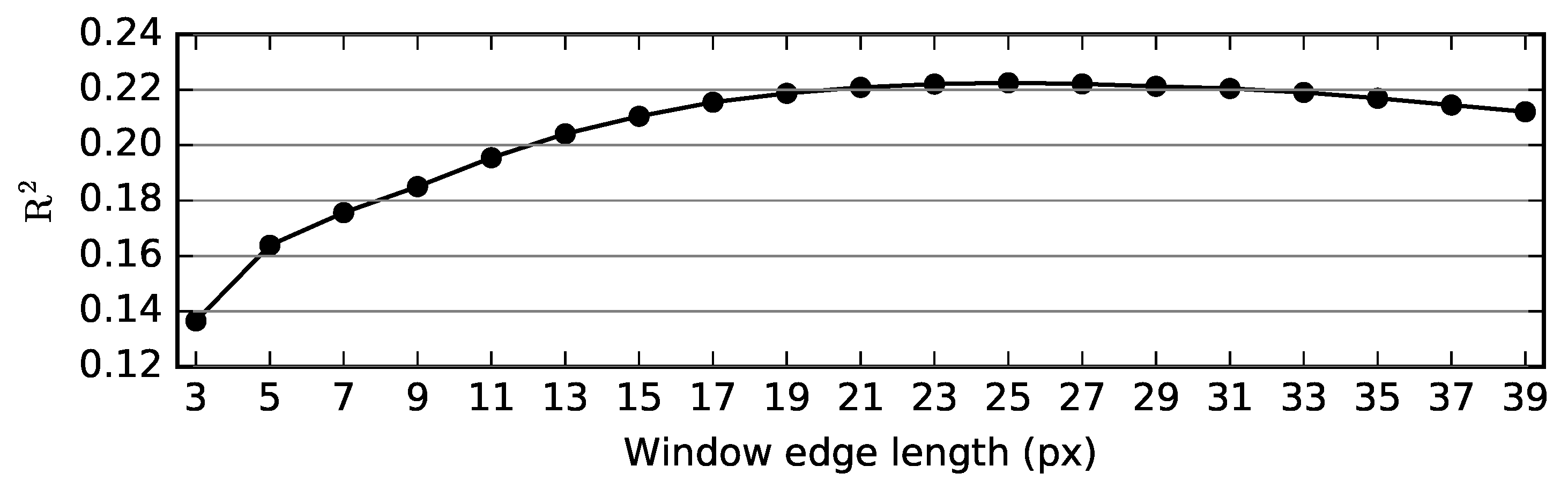
Figure 6.
Results of the feature elimination. Bars denote averages, error bars denote standard deviations of the scores reached during all runs for each scene in the tuning dataset.
Figure 6.
Results of the feature elimination. Bars denote averages, error bars denote standard deviations of the scores reached during all runs for each scene in the tuning dataset.
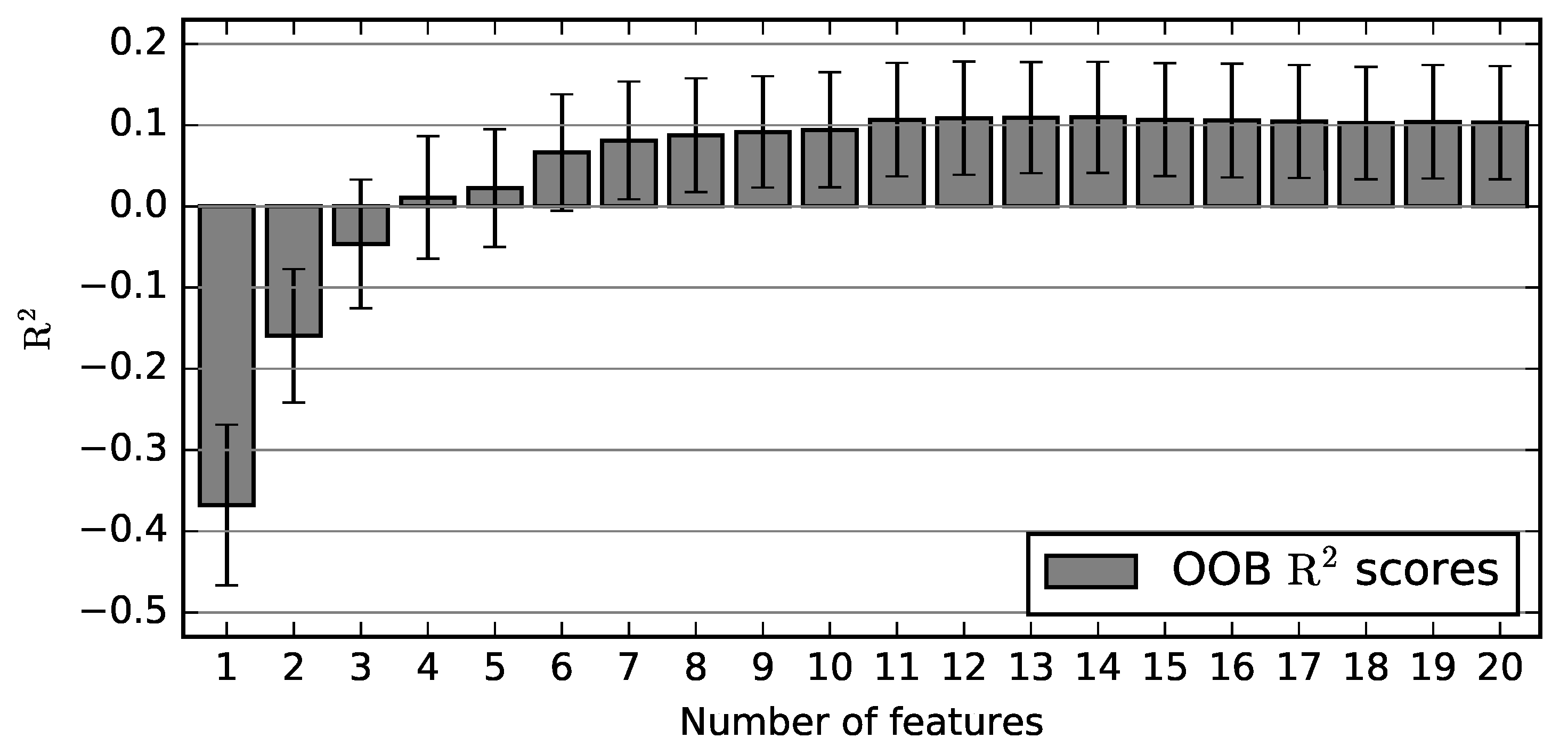
Figure 7.
Average feature importances and standard deviations relative to ELV (100) of the 14 input features used for the final RF model generations. Feature importances were calculated for all 11’993 sample MSG scenes from the tuning data set using all input features.
Figure 7.
Average feature importances and standard deviations relative to ELV (100) of the 14 input features used for the final RF model generations. Feature importances were calculated for all 11’993 sample MSG scenes from the tuning data set using all input features.

Figure 8.
RF parameter tuning results for between 1 and 5 and between 50 and 300. (a) shows scores and (b) shows processing times per MSG scene for the different RF parameter settings.
Figure 8.
RF parameter tuning results for between 1 and 5 and between 50 and 300. (a) shows scores and (b) shows processing times per MSG scene for the different RF parameter settings.
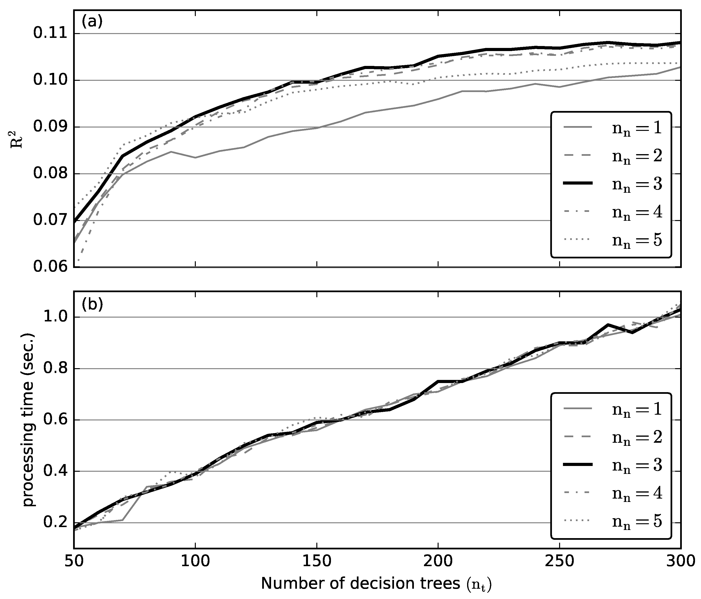
Figure 9.
The basic steps of the fog retrieval scheme at the example of 15 November 2011 00:00 UTC. The background of each subplot is an IR composite of the 3.9 μm, 10.8 μm and 12.0 μm band. The domain is cropped to Central Europe in order to make small scale patterns visible. (a) shows a combination of ground truth and satellite data. Circles mark positions of CBA reporting stations. Colors denote observed CBAs. Black dots indicate that no CBA was measured at the given time. (b) displays RF predictions for all cloud-covered regions above land. (c) presents the final fog derivation (blue areas) and station observations (colored circles). Blue circles mark stations with fog occurrence, yellow circles mark stations where fog formed or dissipated during the recording of the satellite scene and red circles mark stations where no fog was observed.


Figure 10.
Hourly variations in LLO cross validation measures averaged over all years and all ground truth stations: (a) MAE of CBA predictions, (b) observed and predicted fog frequencies as well as PC, (c) POD, FAR and HSS.
Figure 10.
Hourly variations in LLO cross validation measures averaged over all years and all ground truth stations: (a) MAE of CBA predictions, (b) observed and predicted fog frequencies as well as PC, (c) POD, FAR and HSS.

Figure 11.
Monthly variations in LLO cross validation measures averaged over all years and all ground truth stations: (a) MAE of CBA predictions, (b) observed and predicted fog frequencies as well as PC, (c) POD, FAR and HSS.
Figure 11.
Monthly variations in LLO cross validation measures averaged over all years and all ground truth stations: (a) MAE of CBA predictions, (b) observed and predicted fog frequencies as well as PC, (c) POD, FAR and HSS.

Figure 12.
Predicted vs. observed fog frequencies for all (a) METAR and (b) SYNOP stations. Values are averaged over the complete period from 2006 to 2015.
Figure 12.
Predicted vs. observed fog frequencies for all (a) METAR and (b) SYNOP stations. Values are averaged over the complete period from 2006 to 2015.

Figure 13.
Fog frequency averaged over the complete period from 2006 to 2015.

Figure 14.
Fog frequency anomalies of (a) 00:00 UTC, (b) 06:00 UTC, (c) 12:00 UTC and (d) 18:00 UTC averaged over the complete period from 2006 to 2015. Anomaly values are given in in percentage points. Blue colors indicate positive values, red colors indicate negative values. Panels (e–h) give the corresponding averaged fog frequency anomalies for the different elevation levels.

Figure 15.
Fog frequency anomalies of the four seasons averaged over the complete period from 2006 to 2015. Anomaly values are given in in percentage points. Blue colors indicate positive values, red colors indicate negative values. (a) Winter: December, January, February; (b) Spring: March, April, May; (c) Summer: June, July, August; and (d) Autumn: September, October, November. Panels (e–h) give the corresponding averaged fog anomalies for the different elevation levels.


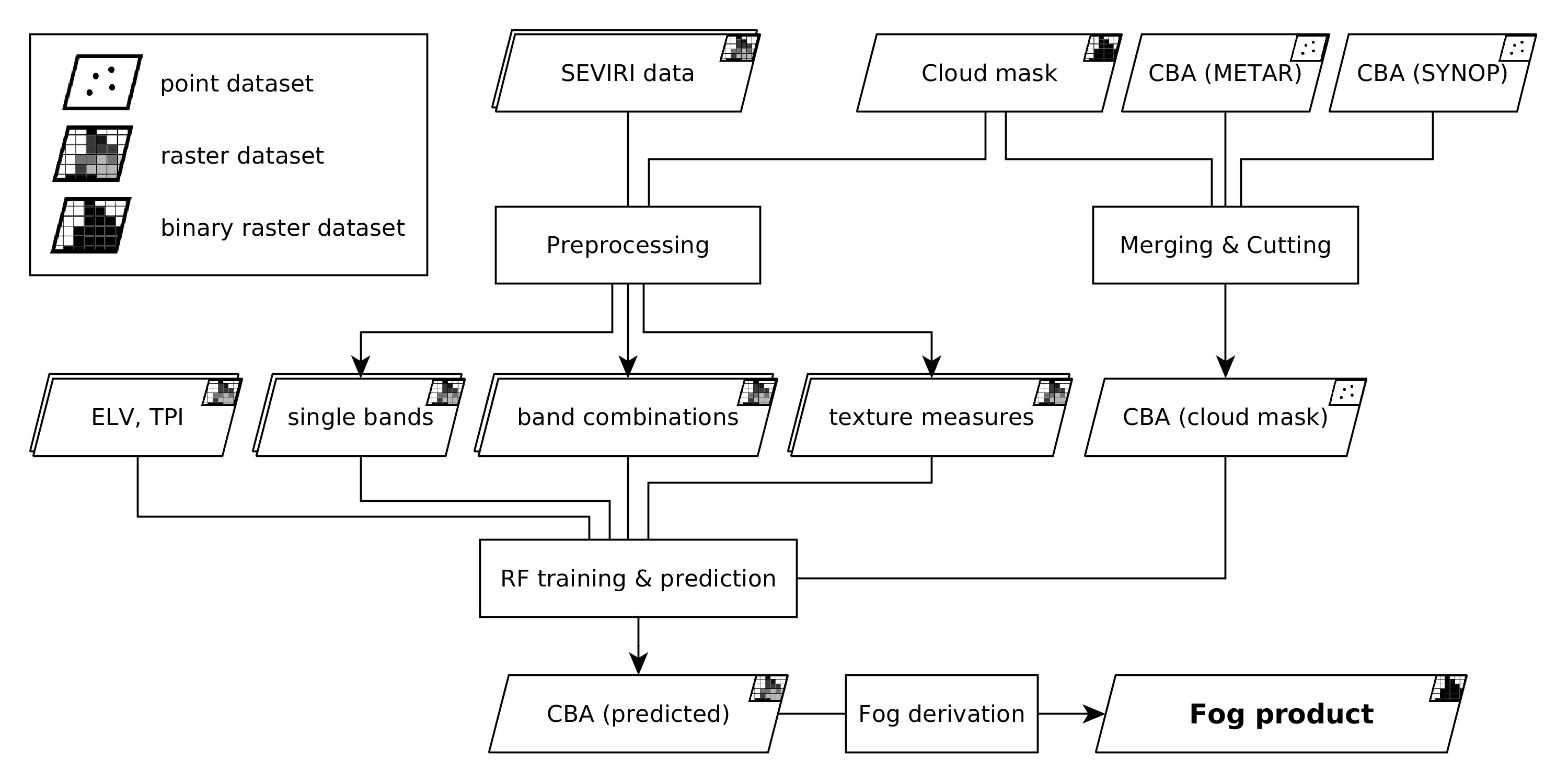
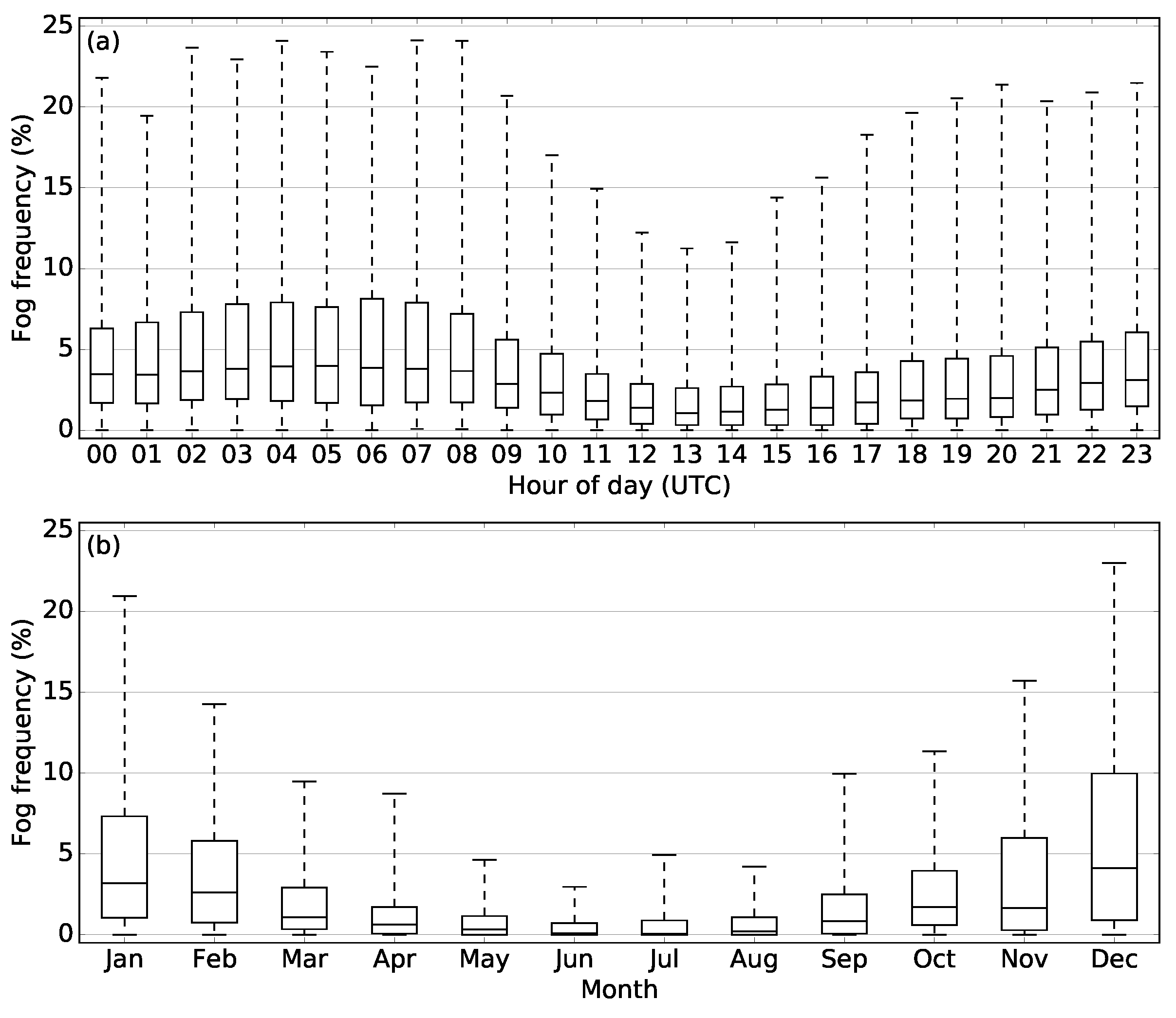
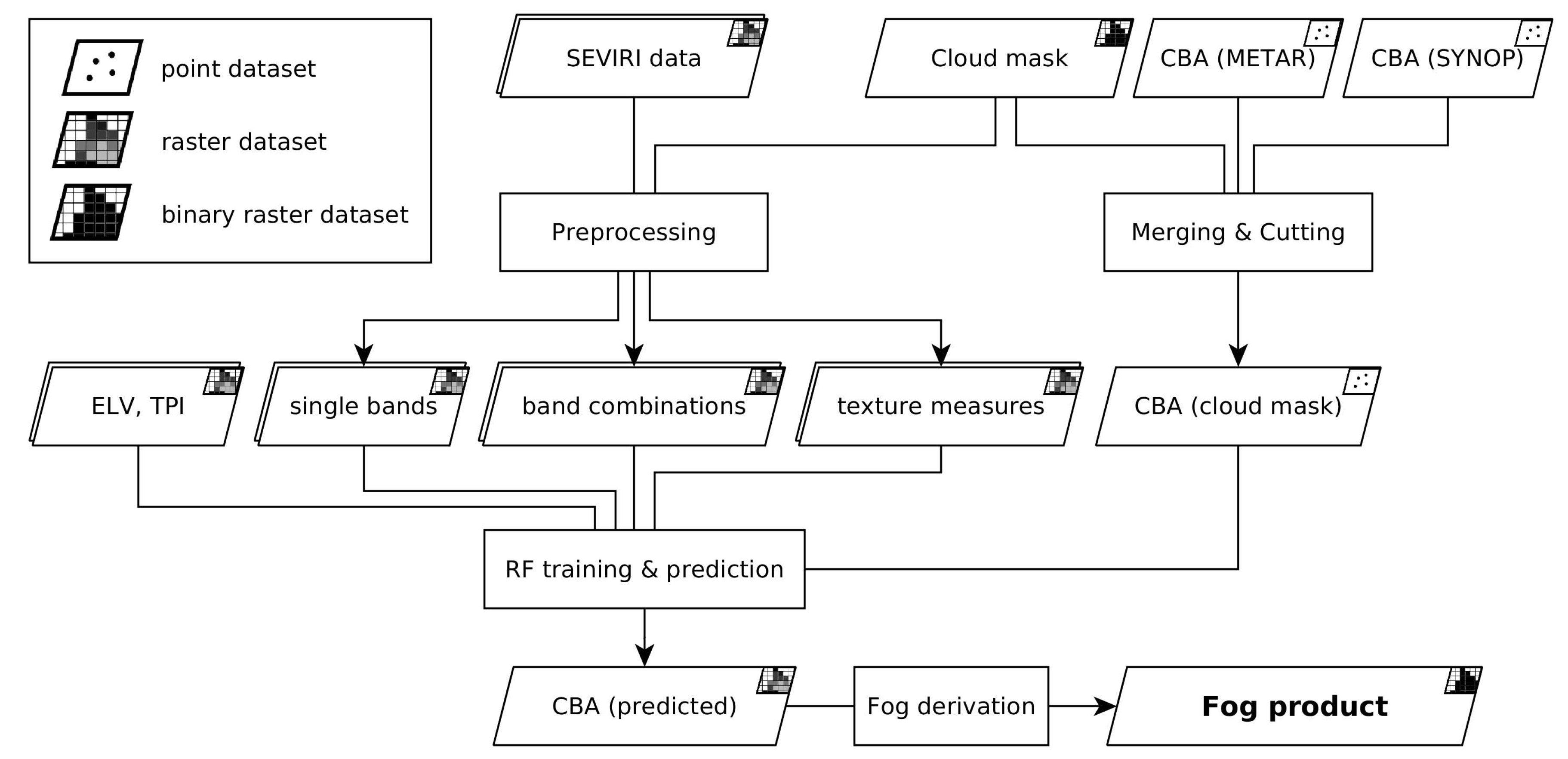
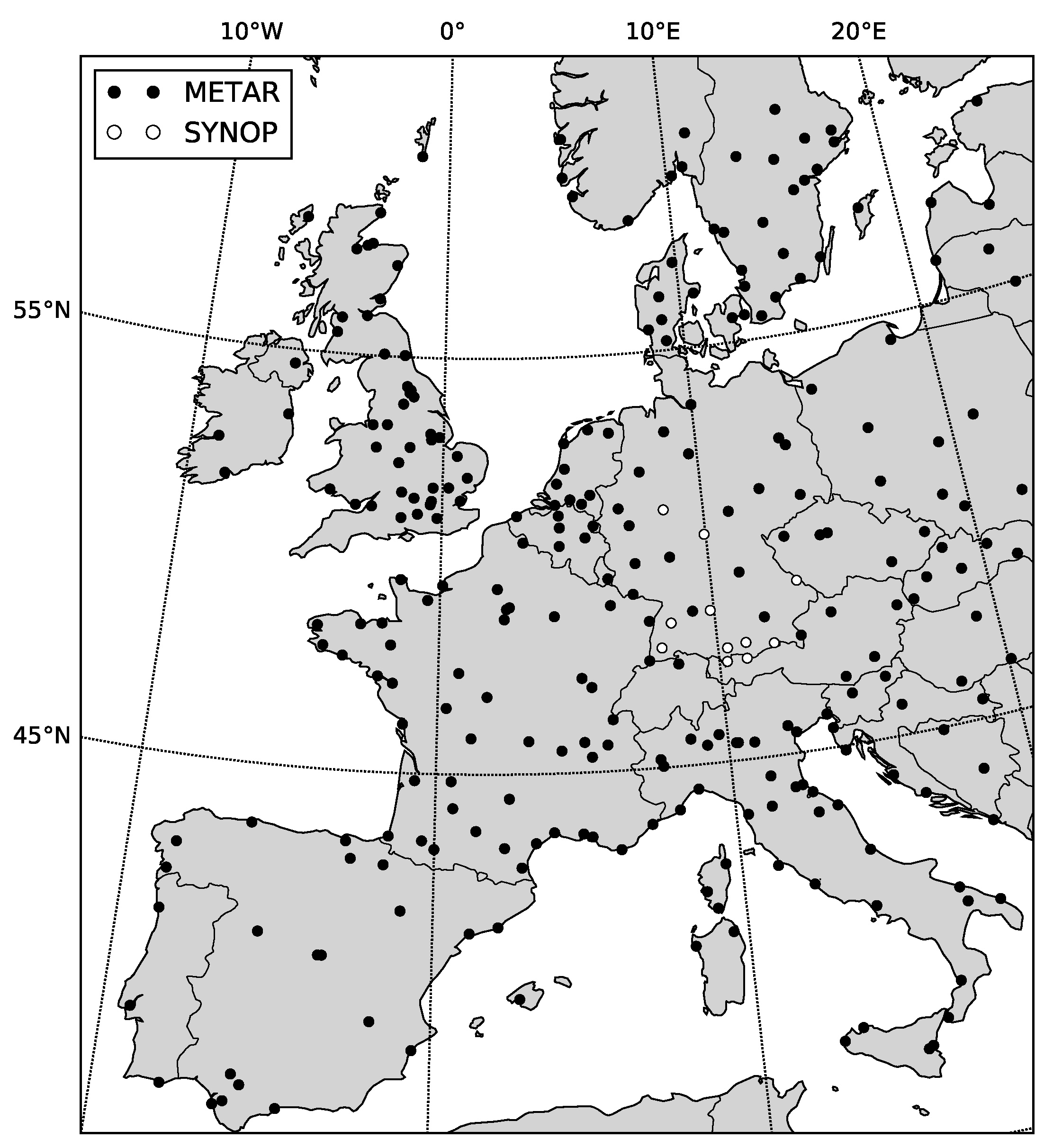
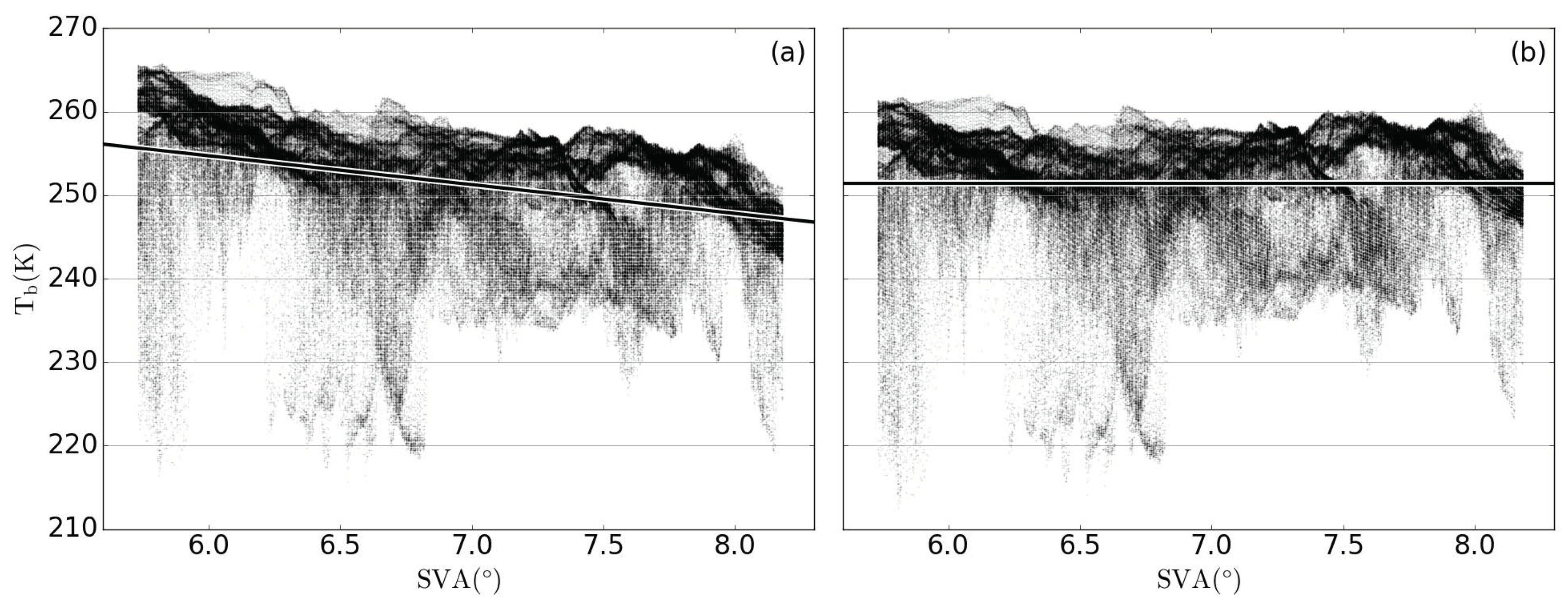
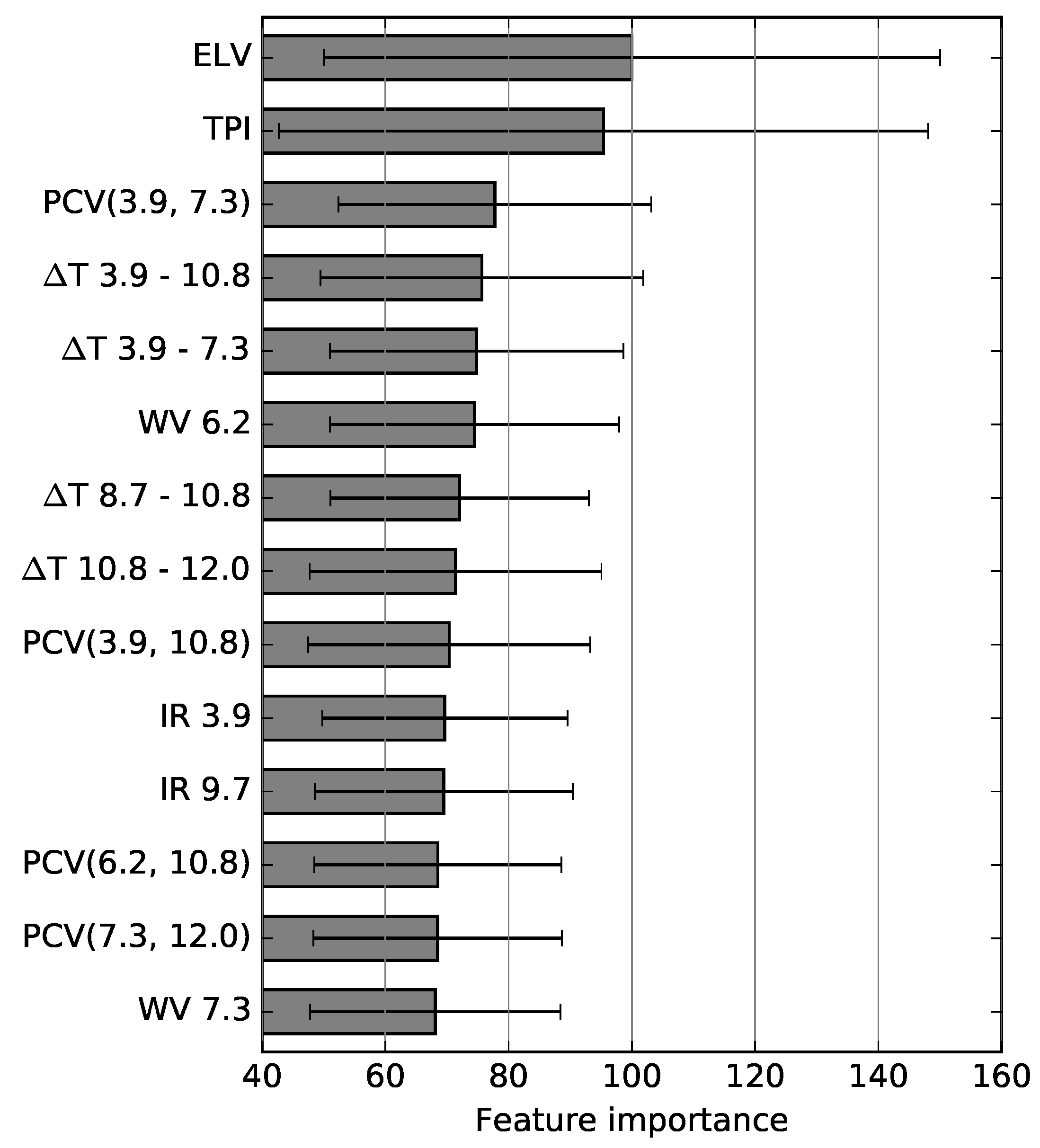
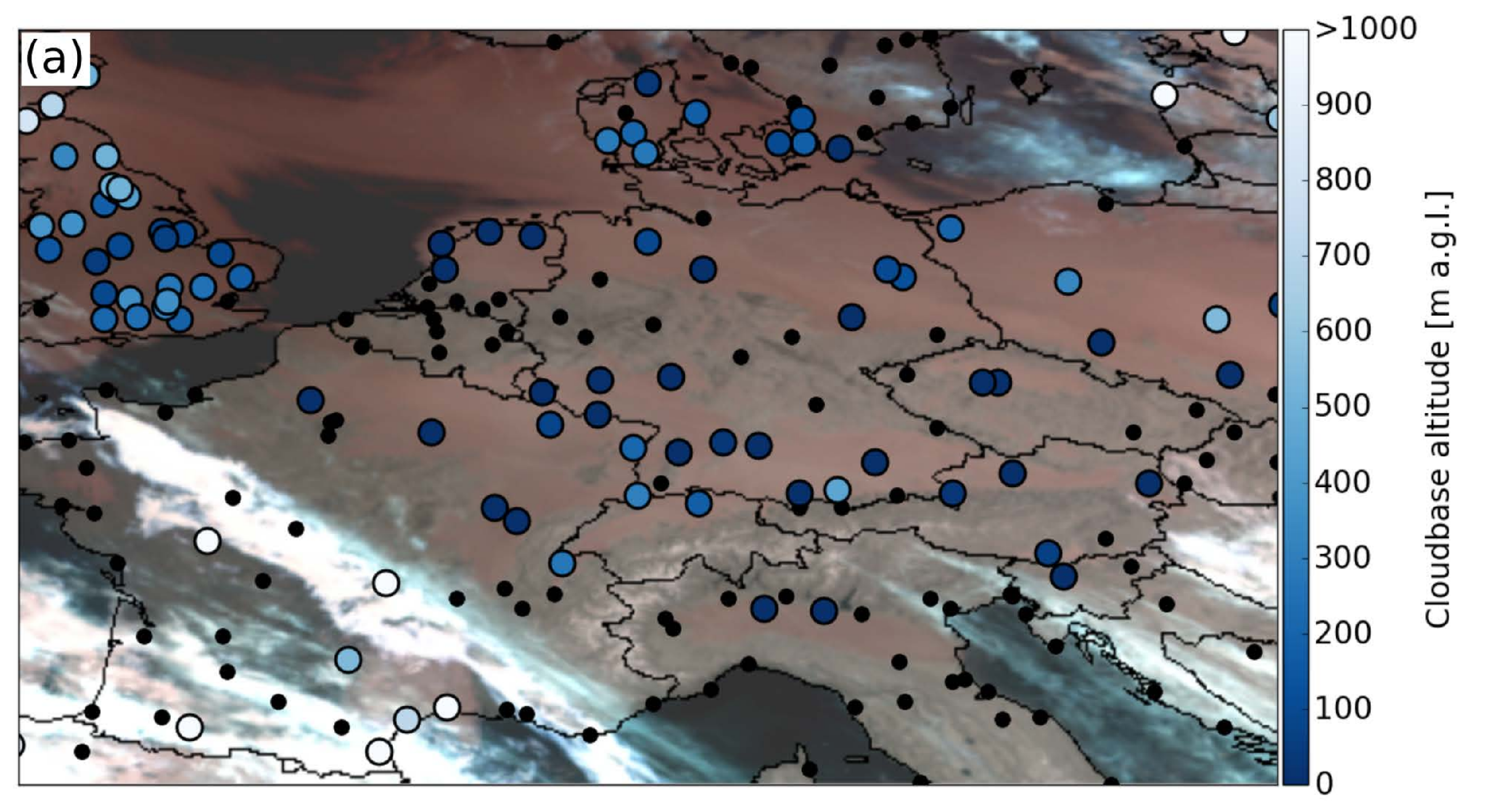
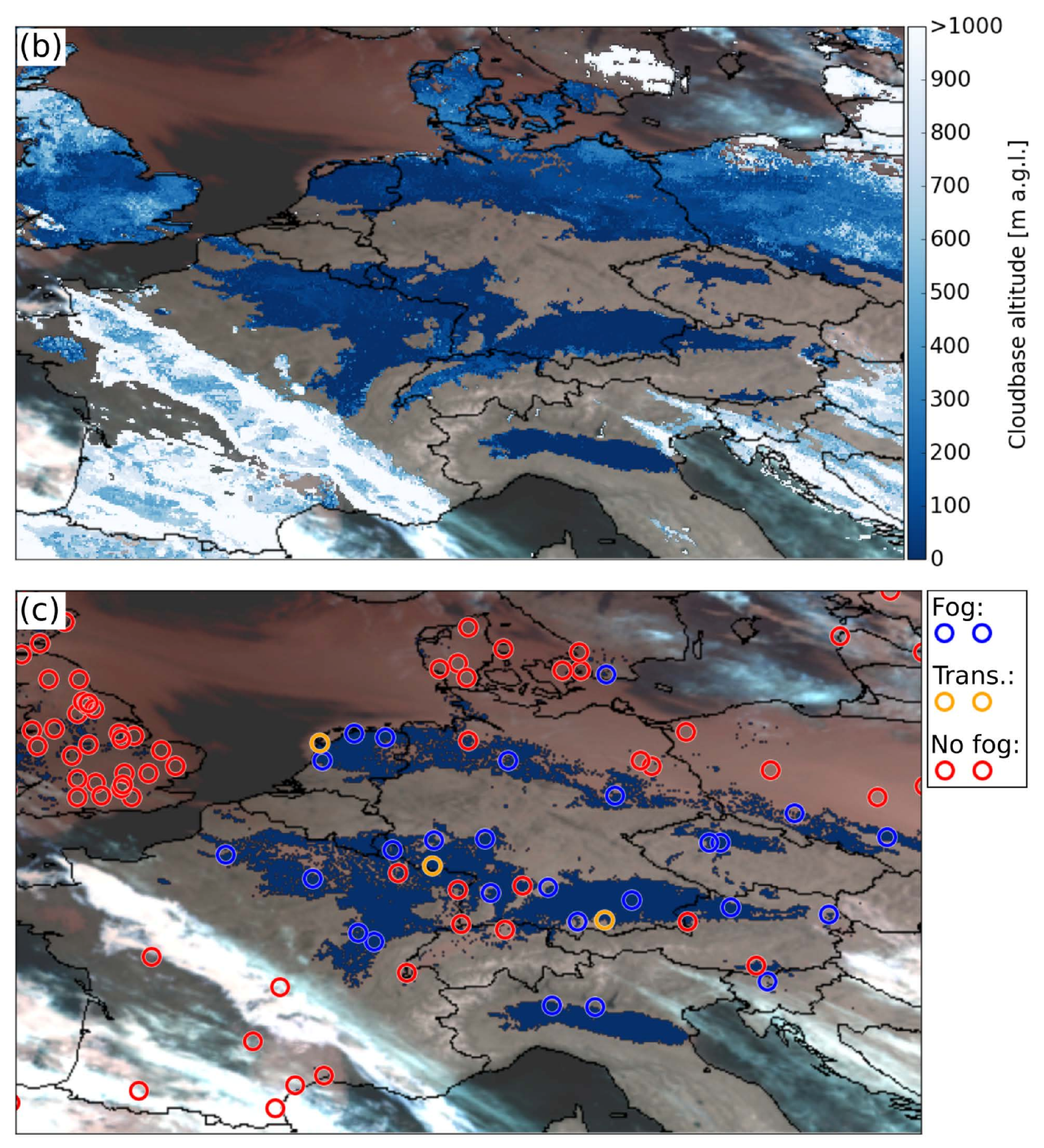
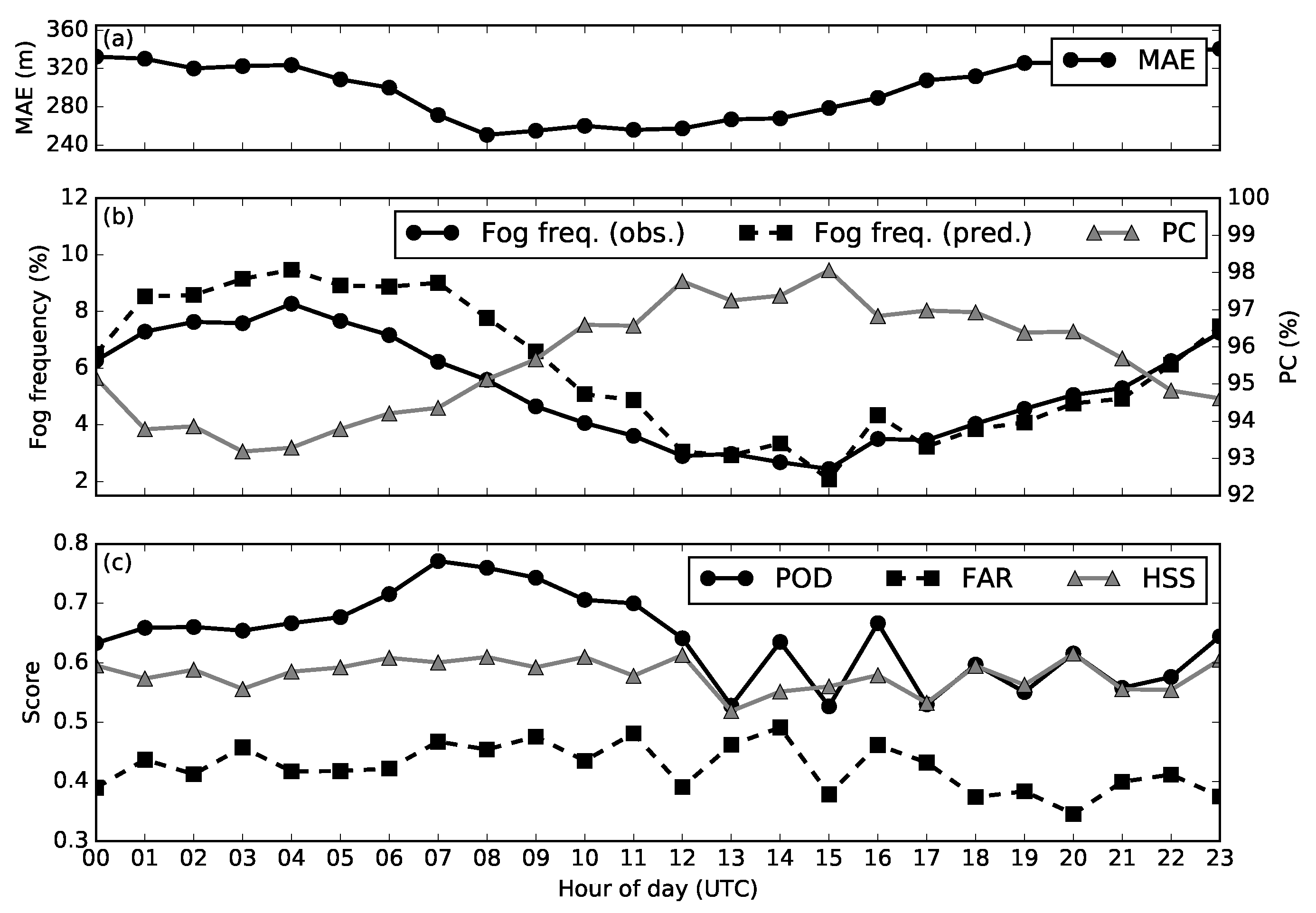
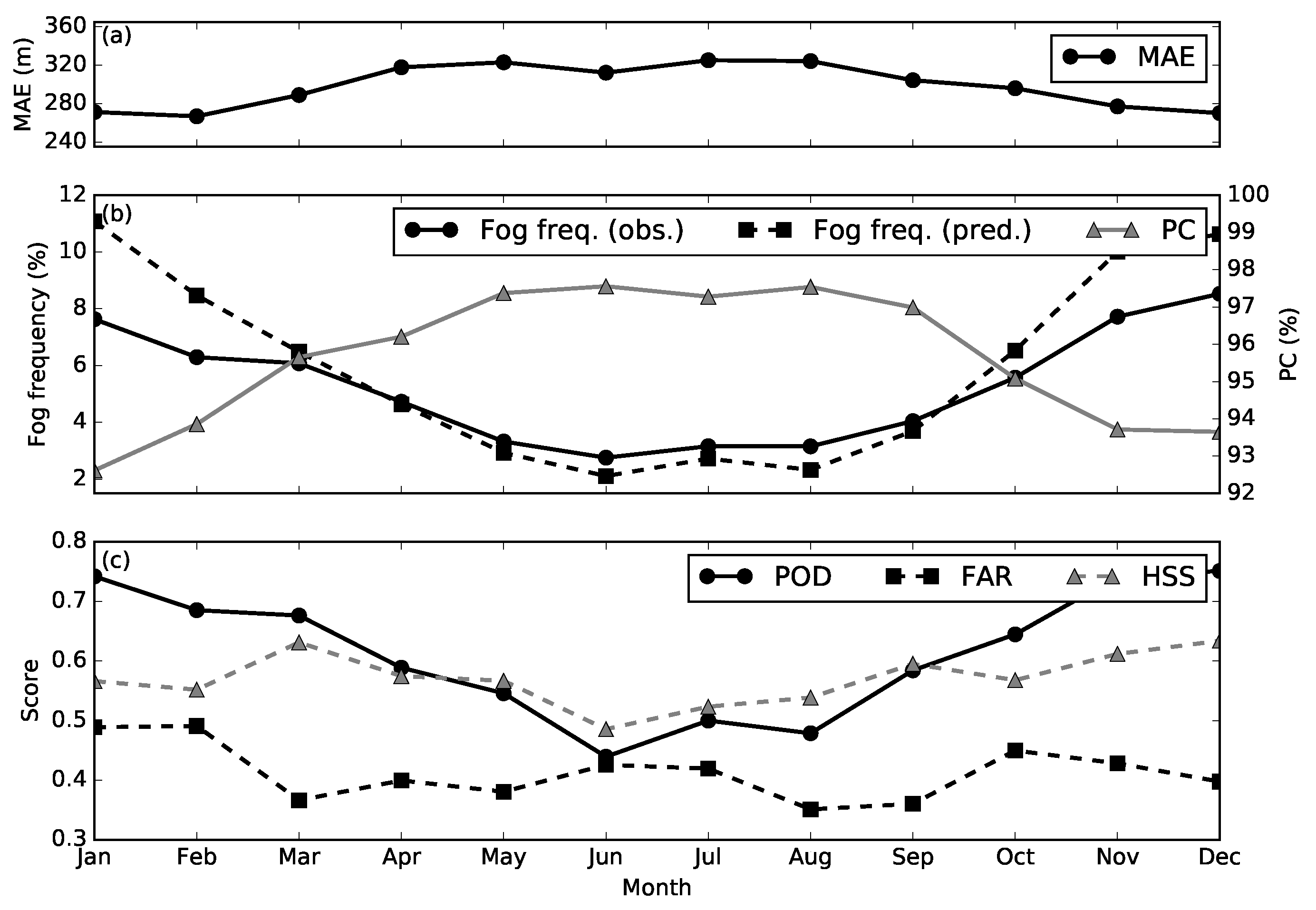
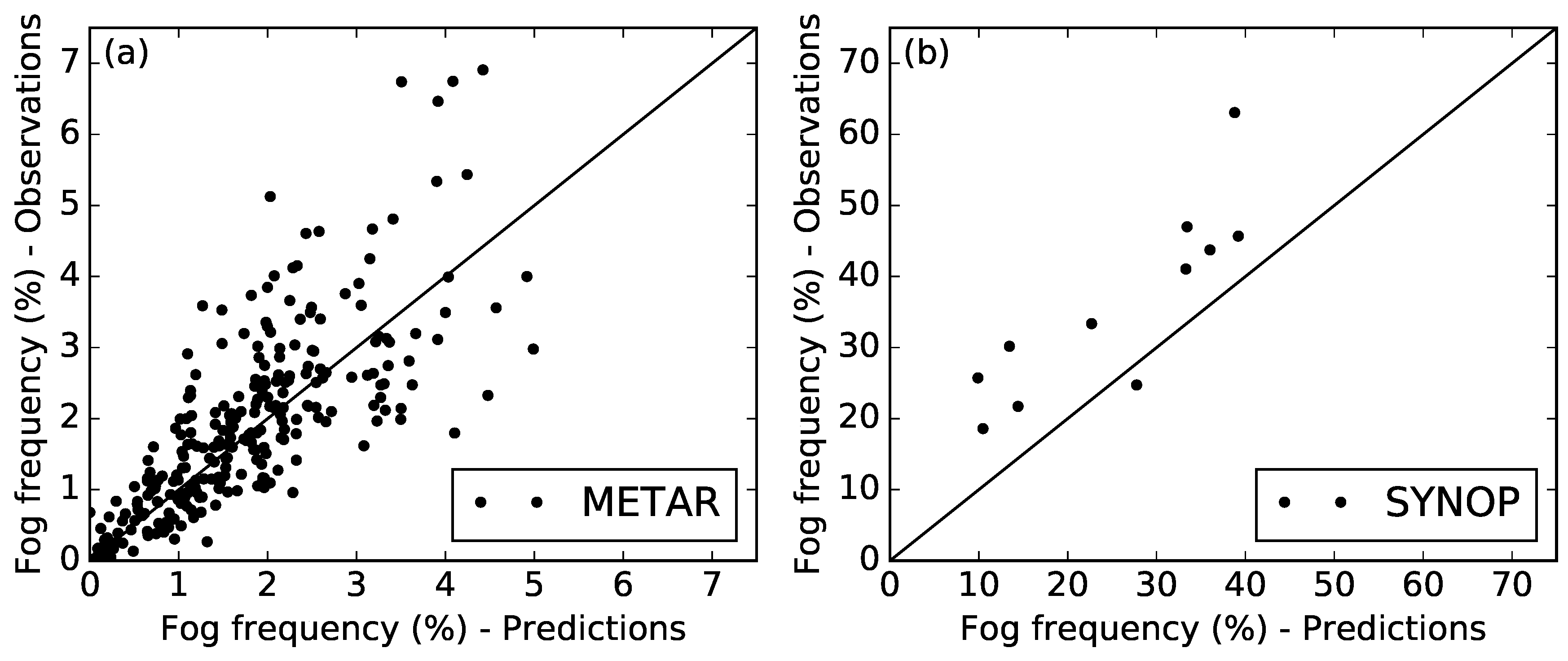
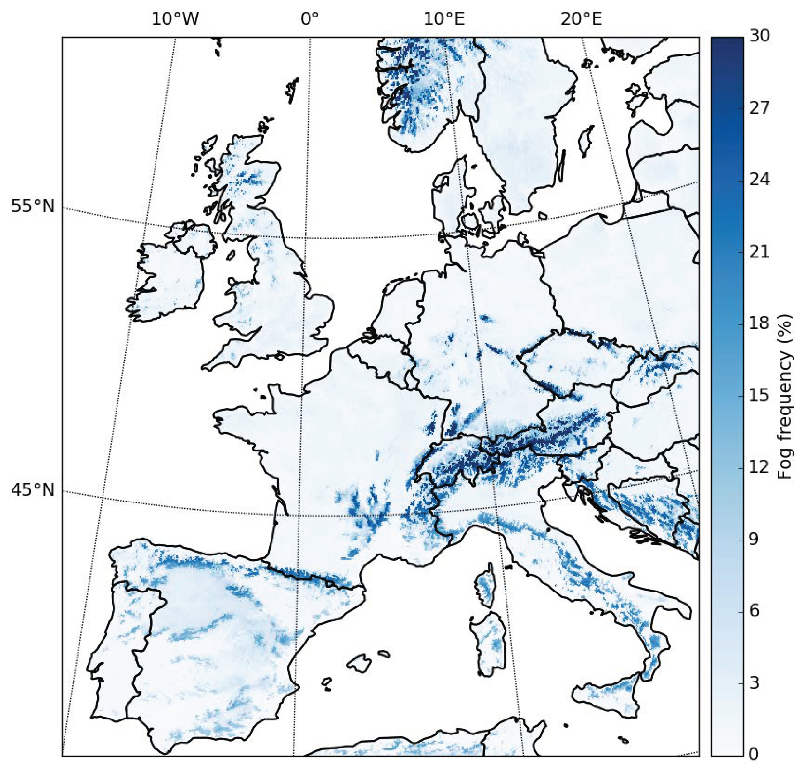
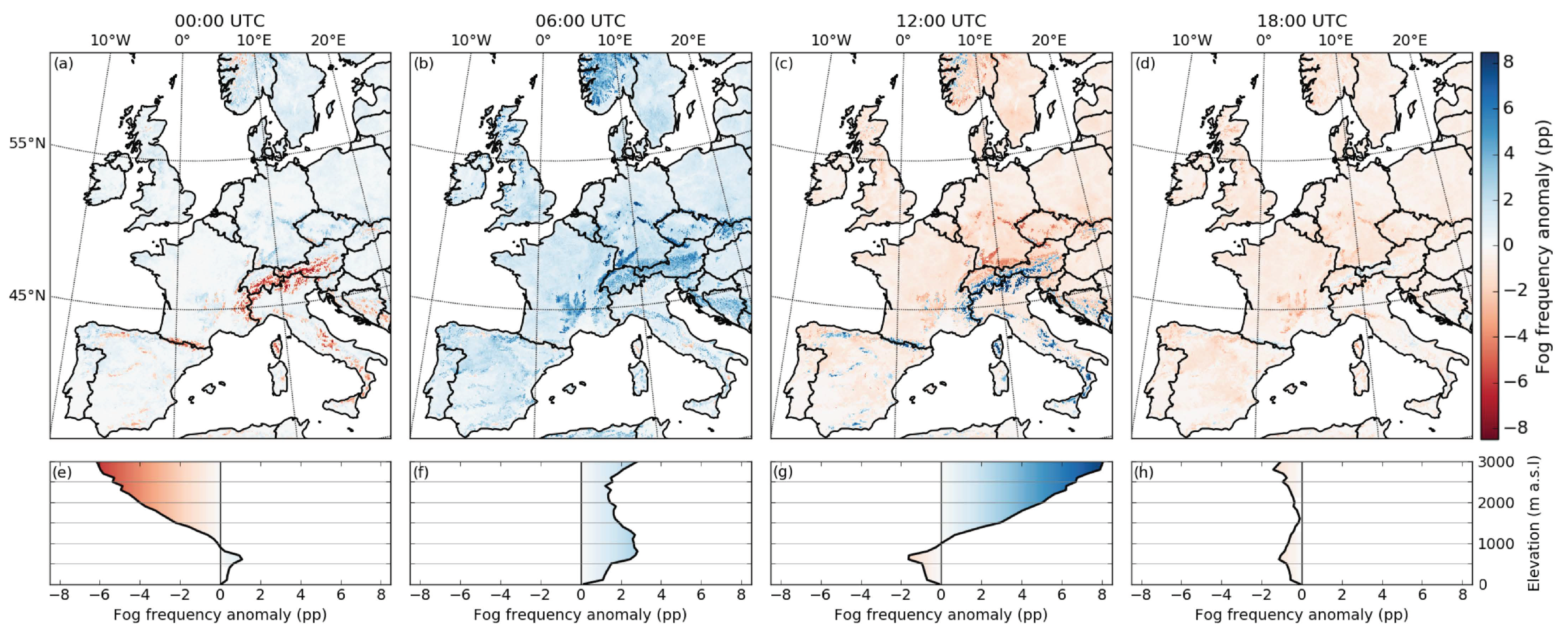
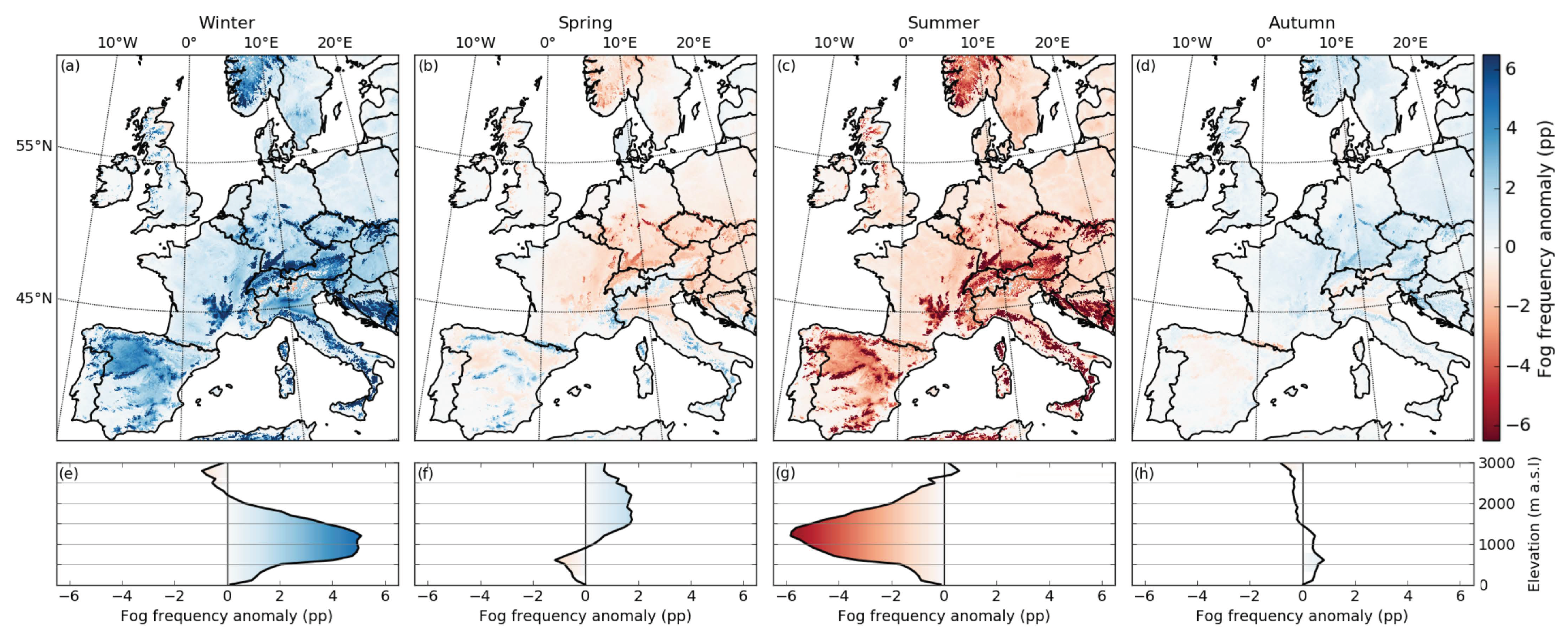
Table 1.
All input features used for RF tuning. MSG bands are denoted with their central wave length in μm.
Table 1.
All input features used for RF tuning. MSG bands are denoted with their central wave length in μm.
| MSG Bands | Derived Data | Static Data |
|---|---|---|
| VIS 0.6 | T 7.3–12.0 | ELV |
| VIS 0.8 | T 8.7–10.8 | TPI |
| IR 1.6 | T 10.8–12.0 | |
| IR 3.9 | T 3.9–7.3 | |
| WV 6.2 | T 3.9–10.8 | |
| WV 7.3 | STD (all bands) | |
| IR 8.7 | VAR (all bands) | |
| IR 9.7 | MAD (all bands) | |
| IR 10.8 | ROD (all bands) | |
| IR 12.0 | CV (all band comb.) | |
| IR 13.4 | PCV (all band comb.) |
Table 2.
Verification measures of SOFOS and the hybrid scheme applied in this study.
| Measure | SOFOS | Hybrid |
|---|---|---|
| PC | 0.99 | 0.95 |
| POD | 0.52 | 0.61 |
| FAR | 0.66 | 0.41 |
| HSS | 0.41 | 0.58 |
© 2018 by the authors. Licensee MDPI, Basel, Switzerland. This article is an open access article distributed under the terms and conditions of the Creative Commons Attribution (CC BY) license (http://creativecommons.org/licenses/by/4.0/).
Share and Cite
MDPI and ACS Style
Egli, S.; Thies, B.; Bendix, J. A Hybrid Approach for Fog Retrieval Based on a Combination of Satellite and Ground Truth Data. Remote Sens. 2018, 10, 628. https://doi.org/10.3390/rs10040628
AMA Style
Egli S, Thies B, Bendix J. A Hybrid Approach for Fog Retrieval Based on a Combination of Satellite and Ground Truth Data. Remote Sensing. 2018; 10(4):628. https://doi.org/10.3390/rs10040628
Chicago/Turabian StyleEgli, Sebastian, Boris Thies, and Jörg Bendix. 2018. "A Hybrid Approach for Fog Retrieval Based on a Combination of Satellite and Ground Truth Data" Remote Sensing 10, no. 4: 628. https://doi.org/10.3390/rs10040628
Note that from the first issue of 2016, this journal uses article numbers instead of page numbers. See further details here.