Large-Area Gap Filling of Landsat Reflectance Time Series by Spectral-Angle-Mapper Based Spatio-Temporal Similarity (SAMSTS)


Geospatial Sciences Center of Excellence, South Dakota State University, Brookings, SD 57007, USA
*
Author to whom correspondence should be addressed.
Remote Sens. 2018, 10(4), 609; https://doi.org/10.3390/rs10040609
Submission received: 9 March 2018
/
Revised: 7 April 2018
/
Accepted: 12 April 2018
/
Published: 14 April 2018
(This article belongs to the Special Issue Science of Landsat Analysis Ready Data)
Abstract
:Landsat time series commonly contain missing observations, i.e., gaps, due to the orbit and sensing geometry, data acquisition strategy, and cloud contamination. A spectral-angle-mapper (SAM) based spatio-temporal similarity (SAMSTS) gap-filling algorithm is presented that is designed to fill small and large area gaps in Landsat data, using one year or less of data and without using other satellite data. Each gap pixel is filled by an alternative similar pixel that is located in a non-missing region of the image. The alternative similar pixel locations are identified by comparison of reflectance time series using a SAM metric revised to be adaptive to missing observations. A time series segmentation-and-clustering approach is used to increase the search efficiency. The SAMSTS algorithm is demonstrated using six months of Landsat 8 Operational Land Imager (OLI) reflectance time series over three 150 × 150 km (5000 × 5000 30 m pixels) areas in California, Minnesota and Kansas. The three areas contain different land cover types, especially crops that have different phenology and abrupt changes due to agricultural harvesting, which make gap filling challenging. Fillings on simulated gaps, which are equivalent to 36% of 5000 × 5000 images in each test area, are presented. The gap filling accuracy is assessed quantitatively, and the SAMSTS algorithm is shown to perform better than the simple closest temporal pixel substitution gap filling approach and the sinusoidal harmonic model-based gap filling approach. The SAMSTS algorithm provides gap-filled data with five-band reflective-wavelength root-mean-square differences less the 0.02, which is comparable to the OLI reflectance calibration accuracy.

1. Introduction
Since the free availability of Landsat data, there has been a rapid increase in the use of Landsat data for time series analyses, typically for change detection, but also for classification and biophysical parameter retrieval [1,2]. The Landsat satellites provide the longest, 45+ years, moderate spatial resolution record of the terrestrial surface. Since the 1982 launch of Landsat 4, each Landsat mission has acquired 30 m data with a 16-day repeat cycle and, for extended periods, there have been two Landsat satellites in orbit nominally providing an eight-day repeat cycle [3]. Landsat data are provided in a global path/row World Reference System (WRS-2), and each approximately 180 × 180 km WRS-2 path/row location is overpassed by a Landsat sensor 22 or 23 times per year [4]. However, a number of sensor, ground station and data communication issues, and variable mission acquisition strategies, reduce the acquisition frequency [3,5,6,7]. These effects, combined with cloud obscuration at the time of Landsat overpass [8,9], result in Landsat reflectance time series that have missing observations at various aperiodic times of any year.
Gap filling of reflectance satellite time series is complex because of a number of factors, including surface cover and condition changes, residual clouds, shadows, atmospheric contamination, and temporal reflectance variations caused by surface reflectance anisotropy and directional illumination and viewing variations [10,11,12]. Landsat-specific methods that fill gaps at individual acquisition dates have been developed. For convenience, they are categorized as temporal interpolation (TI) and alternative similar pixel (ASP) gap filling approaches and are reviewed in Section 2.
In this paper, a new ASP gap filling algorithm, which is designed specifically to fill large gaps in Landsat data and work reliably over complex (spatially- heterogeneous and temporally dynamic) surfaces and using one year or less of Landsat data, is described and demonstrated. It uses a similarity metric based on a form of the spectral-angle-mapper (SAM) metric that is adaptive to missing observations in time series and has been demonstrated over temporally-dynamic agricultural areas [13]. It searches for alternative similar segments using a time-series-based segmentation-and-clustering method, and the ASP search window size is not spatially constrained, which makes it suitable for large-area gap filling. The proposed SAM based spatio-temporal similarity (SAMSTS) gap-filling algorithm is demonstrated using 26 weeks (i.e., six months) of Landsat 8 time series data projected into a tiled georeferenced coordinate system. Three 150 × 150 km (5000 × 5000 30 m pixels) test areas over agricultural regions in Minnesota, Kansas and California are considered, which include various crops and other land cover types, including grassland, shrub, forest and urban areas. Simulations removing different pixel areas followed by gap-filling are undertaken to provide insights into the gap-filling algorithm performance. The results are compared qualitatively and quantitatively with the more-straightforward closest temporal pixel substitution gap filling approach and the sinusoidal harmonic model temporal interpolation gap filling approach.
2. Satellite Gap-Filling Literature Review
Methodologies to “fill” gaps in satellite-retrieved reflectance time series were developed initially for systematically-acquired coarse-resolution satellite data acquired by the Advanced Very High Resolution Radiometer (AVHRR) and the Moderate Resolution Imaging Spectroradiometer (MODIS) that provide near-daily global coverage due to their polar low earth orbit and wide (110°) field of view. Compositing procedures were developed to provide reflectance and vegetation index datasets that represent the surface over consecutive n-day time periods [14,15,16]. Compositing approaches have also been developed for Landsat data, but are typically less reliable because the cloud-free observation frequency is lower than provided by near-daily coarse resolution polar orbiting satellite data [17,18,19]. Compositing approaches that invert a bi-directional reflectance distribution function (BRDF) model against n-days of reflectance observations to estimate the reflectance at nadir view and for a consistent solar zenith have been developed as well [20,21]. However, these more physically-based compositing approaches do not work reliably with Landsat data because of the narrow (15°) Landsat field of view that precludes representative sampling of the surface BRDF [22,23].
Coarse-resolution satellite data have been used to help fill gaps in Landsat time series. For example, Roy, D.P. et al. [24] developed a semi-physical fusion approach that used the MODIS BRDF 500 m product to predict 30 m Landsat spectral reflectance for a desired date. Other empirical approaches have been developed based on the spatial and temporal adaptive reflectance fusion model (STARFM) that blends 16-day 30 m Landsat with near-daily or daily 500 m MODIS data to generate synthetic daily Landsat-like 30 m reflectance data [25]. These include methods that are somewhat adaptive to land surface change such as the spatial temporal adaptive algorithm for mapping reflectance change [26], and the spatial and temporal data fusion approach (STDFA) [27]. The enhanced STARFM [28] was developed to handle complex and heterogeneous landscapes by incorporating spectral unmixing and has been demonstrated over agricultural areas [29,30,31]. However, coarse-resolution satellite data that may not always be available or cloud-free, for example, prior to the launch of MODIS in 1999, global coverage near-daily coarse-resolution data suitable for gap-filling Landsat are not available.
Temporal interpolation (TI) gap-filling approaches have been developed that fit time series statistical models to predict reflectance or vegetation index values on a given day. Linear, logistic, or sum of sinusoidal models have been used [32,33,34,35,36,37,38,39]. The model fits are conducted on individual pixel time series. Model fitting is sensitive to the quality, number of available observations, and the seasonality of missing observations. TI methods are typically less reliable for surfaces that have abrupt changes, for example, due to land cover change, flooding, fire, or for surfaces with complex phenology, such as double or triple agricultural cropping [35,40,41]. Time series change detection methods that account for both abrupt and gradual trends in coarse spatial resolution data have been developed [41], but are less well suited for Landsat application as they require a higher observation frequency than provided by Landsat.
The ASP gap-filling approach fills a gap pixel with the values of one or more alternative pixels selected from non-missing pixels found usually in the same image. Alternative similar pixel locations are identified from a reference image that may be the same, a previous, or a subsequent image that has no gap at the location to be filled [42,43,44,45,46,47,48,49,50]. The ASP method was first developed to fill gaps in Landsat 7 Enhanced Thematic Mapper Plus (ETM+) images introduced by the Scan Line Corrector (SLC) failure that occurred in 2003. Landsat 7 ETM+ images with the SLC failure, usually referred to SLC-off images, have 22% less ETM+ image pixels with missing wedge-shaped gaps [5]. The earliest ASP approach used a segmentation map generated from a pre-2003 Landsat 7 ETM+ image without gaps that was overlain on the spatially-coincident SLC-off image [42]. For each band, the missing pixel values were replaced by the majority non-missing pixel values falling in the segment from the same SLC-off image. This was later improved by using a multi-scale segmentation [43]. The strength of this approach is that the gaps are filled with coincident spectral values from the same Landsat image. However, it requires a segmentation that should reflect the surface conditions of the image to be gap filled, which is difficult to obtain everywhere and for all times, and so this is not usually a reliable method. Other ASP methods find alternative similar pixels in local search windows centered on the gap pixel location. For example, Pringle et al. [44] derived the gap pixel value by kriging alternative similar pixel values and locations in the gap image, and also by co-kriging the alternative similar pixel values in both the gap image and previous and/or subsequent reference image(s) when insufficient alternative similar pixels were available. Similarly, Chen et al. [45] derived the gap pixel value as the weighted average of the alternative similar pixels on the gap image. The weight was determined by the spatial distances of each alternative similar pixel to the gap pixel location and the root-mean-square difference of the alternative similar pixel values in the gap image and the reference image. More recent approaches have used Landsat time series. Malambo and Heatwole [49] described a pixel-time-series-comparison-based ASP method to estimate missing spectral-index data and provide gap filling under both gradual and abrupt surface change conditions. They used Landsat time series of a spectral index suitable for burned area discrimination, and alternative similar pixels were identified using a similarity metric that measured the maximum difference between two pixels’ index time series after removing their mean index difference. The filling was conducted iteratively within a search window no more than 41 pixels around the gap pixel location, with gaps progressively “eroded” until they were completely filled. Other researchers have noted that progressive filling in this manner may propagate filling errors and so is less suitable for filling spatially-extensive gaps with heterogeneous land covers [50,51,52].
Large gaps frequently occur in Landsat time series due to extensive regions of cloud obscuration [8,9] and swaths of missing observations caused by the Landsat sensing and orbit geometry [53]. Development of gap-filling methods that can fill large gaps is expected to be particularly difficult over heterogeneous and rapidly-changing areas. Heterogeneous areas have a greater likelihood of containing pixels with fewer available alternative similar pixels [43,47]. For example, adjacent agricultural fields may contain the same crop, but may have a variety of spatial surface variations associated with soils, drainage, irrigation, topography, sowing, harvest date, and growth stage differences that are evident at moderate resolution [54,55]. Similarly, if time series reference data are used, then the reference images are less likely to be similar to the image to be gap filled if the surface land cover and/or condition changes [26,28]. Despite these issues, the ASP approach does not require contemporaneous coarser resolution satellite data that may not be available or cloud-free. Further, unlike TI approaches, the ASP approach makes no assumptions concerning the surface temporal variation and does not require long-term (i.e., annual or multiple year) time series. These observations motivate the SAMSTS algorithm that uses an ASP approach and is described below.
3. Data
3.1. Landsat 8 Data
Landsat 8 Operational Land Imager (OLI) data, which were processed in a similar manner to the recently-available Landsat Analysis Ready Data (ARD) data [56], were used in this study. Images for 26 weeks (six months) sensed from 28 April to 26 October 2013 were used. The reflectance band data were converted to surface reflectance using the established Landsat Ecosystem Disturbance Adaptive Processing System (LEDAPS) code that uses aerosol characterizations derived independently from each Landsat acquisition and assumes a fixed continental aerosol type and uses ancillary water vapor data [57]. The Landsat 8 quality assessment band was used to liberally remove cloud-contaminated pixels, defined in this study as medium and high confidence cloud pixels and high confidence cirrus pixels. The Landsat 8 OLI data are acquired over a 15° field of view and so small bi-directional reflectance effects (due to viewing and solar geometry variations and surface reflectance anisotropy) are present [23,58], but they were not corrected for in this study. Only the OLI surface reflectance for the green (0.56 μm), red (0.66 μm), near-infrared (NIR) (0.87 μm), and two shortwave infrared (SWIR) (1.61 μm and 2.20 μm) bands were used; the shorter wavelength Landsat 8 OLI blue bands were not used because atmospheric correction is considerably less reliable at shorter blue wavelengths [59,60].
Gridded atmospherically-corrected weekly Landsat 8 OLI data were generated using the Web-Enabled Landsat Data (WELD) processing system [17]. The WELD data are defined in the Albers Equal Area projection in 5000 × 5000 30 m pixel tiles, which was adopted to generate the ARD [56,61]. These data have been used previously for large-area time series land cover and surface change mapping applications [62,63,64,65,66]. At CONUS latitudes, the sensed Landsat 8 image swaths do not spatially overlap in any calendar week [53]. In the weekly CONUS WELD time series, like the ARD, a fixed pixel location may be sensed seven or nine days apart due to the orbit and sensing geometry.
3.2. Cropland Data Layer
The United States Department of Agriculture (USDA) National Agricultural Statistics Service (NASS) Cropland Data Layer (CDL) product was used to provide insights into the results and to understand the land surface dynamics in terms of the dominant land cover classes. The CDL is generated annually using moderate-resolution satellite imagery and extensive agricultural ground truth via a supervised non-parametric classification approach. It defines about 110 land cover and crop type classes at 30 m for all the CONUS in the same Albers Equal Area conic projection as the WELD data and the ARD [67,68]. The CDL for 2013 was used as it is the same year as the Landsat 8 OLI data used in this study and was obtained from [69].
4. Test Areas
Three WELD/ARD 150 × 150 km (5000 × 5000 30 m pixel) tiles located in California, Minnesota and Kansas were selected as test areas. The tiles are representative of different land cover types (Figure 1) with seasonally dynamic and different land covers (Figure 2), and have representative amounts of missing data including large spatial gaps (Table 1). The California tile (Figure 1a) is in Northern California, encompassing Colusa and San Joaquin counties, and has the greatest number of land cover classes, but relatively less pronounced phenological variations due to its more temperate climate. The Minnesota tile (Figure 1b) encompasses the southwest corner of Minnesota and parts of Northern Iowa. The Kansas tile (Figure 1c) is in the southwest of Kansas and encompasses parts of Northern Oklahoma. The Minnesota and Kansas tiles are predominantly agricultural and are located in the U.S. corn belt [70,71] and wheat belt [72], respectively.
Figure 2 illustrates the mean weekly Normalized Difference Vegetation Index (NDVI) for the major CDL classes in each test area. Phenological variations among the CDL classes occur due to a number of factors, including geographic location, weather and site conditions, crop planting and harvesting dates, and land cover differences. The NDVI profiles typically have unimodal distributions with pronounced spring and summer NDVI peaks. In the California tile, except for the CDL corn and rice classes, there is relatively less pronounced phenological variation. The summary values illustrated in Figure 2 do not clearly reflect gaps, except for weeks 18, 20, 23, and 39 (California), weeks 21, 22, 24, and 34 (Minnesota), and weeks 19, 21, 25, 32, 37, and 42 (Kansas), when there were no Landsat acquisitions due to the location of the tiles relative to the Landsat 8 ground track.
Table 1 summarizes the number of missing pixel observations (i.e., cloudy or not sensed) over the three tiles for the 26 weeks of 2013. The left column summarizes the number of weeks with at least one valid 30 m pixel in the tile, denoted by n. The percentage of missing weekly 30 m pixels is summarized in two ways: as the sum of the number of missing 30 m pixels observations in each weekly tile divided by the product of 26 and the tile spatial dimensions (Table 1, middle column); and as the sum of the number of missing 30 m pixels observations in each weekly tile divided by the product of n and the tile spatial dimensions (Table 1, right column). Over the 26 weeks, about 50% of the study area data were missing but, when considering only those weeks with at least one valid pixel, the percentage is 41% (California), 46% (Minnesota), and 30% (Kansas).
5. Gap-Filling Methodology
5.1. Overview
Figure 3 illustrates the workflow of the SAMSTS algorithm. It can be summarized by several steps. First, the input Landsat multispectral time series images are considered together and segmented (across time and space) into a single segmentation image. The resulting segments are divided into two groups (≥3 pixels and <3 pixels) for the subsequent processing. The segments (in either group) are clustered, and each segment is associated to M clusters. Then, the gap filling is undertaken for a specified target image in the time series that has missing pixels. For each segment (Sgap) with one or more missing pixels in the target image, an alternative similar segment (), which has valid non-missing pixel values in the target image, is identified using the cluster information. Then, for each missing pixel in segment Sgap, its alternative similar pixel is identified within and is used to fill the gap pixel’s values.
A refined spectral angle mapper similarity metric (SAMr) is incorporated in the steps of the time series segmentation, segment clustering, and identification of alternative similar segments and pixels in the target image. This measure is based on the spectral angle mapper (SAM) that is used conventionally to determine the spectral similarity between two pixels by calculating the cosine of the angle subtended between their points in feature space and the feature space origin [73,74,75]. Previously, we refined SAM to allow the comparison of two single-pixel Landsat multispectral time series with missing temporal observations [13] as:
where and are two vectors whose feature space values are defined by xz∈[1…n], and n (≥2) is the number of feature space dimensions, i.e., the product of the number of spectral bands and the number of images in the time series; is a step-function returning 1 if both and are non-missing observations and returning 0 otherwise. Thus, SAMr0 measures the similarity between two pixels’ time series considering only their temporally-corresponding non-missing observations. SAMr0 is bounded in the range [0,1], tends to 1 as the time series values of the two pixels become similar, and is 1 when the time series values are identical. However, where there is a high proportion of missing observations, then only a small number of temporally-corresponding observations will be available, which will reduce the reliability of SAMr0. To minimize the impact of this issue, the SAMr is used:
where SAMr0 is defined by Equation (1), n′ is the number of temporally-corresponding observations between and , n is the number of feature space dimensions, i.e., the product of the number of spectral bands and the number of images in the time series (5 × 26), and the term is the mean difference between the two time series’ temporally-corresponding observations. Like SAMr0, the SAMr is bounded in the range [0,1] and equals 1 when the time series are identical.
In this study, obs50% in Equation (2) is set as the percentage of non-missing tile 30 m pixel observations over the 26 weeks multiplied by the product of the number of weeks (26) and the number of bands (five Landsat bands, Section 3.1) times 0.5. For example, for the California study area, 47.5% of the tile 30 m pixel observations over the 26 weeks are missing (Table 1, middle column) and so obs50% is 34 (derived as ((100 − 47.5)/100) × 26 × 5 × 0.5). Thus, the misalign penalty term occurs for the California gap-filling when the five-band 26-week vectors and have less than 34 temporally-corresponding values. If there are more temporally-corresponding values, i.e., n′ is high, then the penalty term is not invoked.
The SAMr is used to compare not only single-pixel time series, but also to compare the mean time series values of pixels that are associated together after the application of a segmentation algorithm. For brevity, we define the term “segment signature” as the mean reflectance values for each of the five Landsat bands over the 26 weeks (i.e., a vector of 130 × 1 mean values). The mean values are derived considering all the non-missing pixels in the segment. The SAMr is then calculated as Equation (2) with and defined by segment signatures or single pixel time series. We also define the term “cluster signature” as the mean of the segment signatures in a cluster. The cluster signature is a vector of 130 × 1 reflectance values.
5.2. The Spectral-Angle-Mapper-Based Spatio-Temporal Similarity (SAMSTS) Gap-Filling Algorithm
The SAMSTS gap filling algorithm utilizes a segment-and-clustering approach that is illustrated in Figure 4. The approach is undertaken as follows: (1) the input time series images are considered together and segmented (across time and space) into a single segmentation (e.g., six segments, Figure 4a); (2) the segments are clustered in an unsupervised manner (e.g., into two clusters denoted by hatched lines in Figure 4b); (3) the SAMr time series calculations are undertaken comparing the segment containing the gap pixel (cross, falling in the red segment with diagonal hatching) with alternative similar segments that belong to the same cluster (diagonal hatching), and the most similar alternative segment that maximizes SAMr is selected; and (4) for each gap pixel in the gap segment, its corresponding alternative pixel is individually searched only among the candidate pixels in the corresponding most similar alternative segment. These four steps are described below in detail through Section 5.2.1, Section 5.2.2 and Section 5.2.3
5.2.1. Time Series Image Segmentation
The input time series images, i.e., 26 weeks of five bands, each 5000 × 5000 pixels, are segmented into a single segmentation map composed of 5000 × 5000 pixels. Conventionally, segmentation algorithms cannot work if there are missing data, or the missing data are not segmented. As Landsat time series contain arbitrarily-distributed gaps across space and time, the segmentation should be adaptive to them. The SAMr is used with a simple region-growing image segmentation method [76]. Each pixel is associated with a spatially-adjacent pixel (considering an 8-connected pixel neighborhood) if the SAMr value of the two pixels’ time series is >0.9995. The 0.9995 threshold is purposefully set high to ensure that pixels belonging to the same segment are highly similar, i.e., have a nearly identical 26 week temporal evolution in the five-band reflectance. This threshold was empirically determined through tests on the input data for the three test areas. Since the agricultural study areas typically have a higher degree of spatio-temporal complexity than most other landscapes [31,51], we anticipate that this threshold will be suitable for general cases when six months of Landsat data are used.
Over-segmentation may occur that reduces the computational efficiency of the algorithm. Consequently, spatially-adjacent similar segments are merged to reduce the number of segments. For each segment, the segment signature is derived as the mean non-missing reflectance for each band over the 26 weeks where the mean is derived considering all the pixels in the segment. Then, for each pixel in the segment, the SAMr between the pixel time series and the segment signature is derived, and for segments composed of more than one pixel, the standard deviation of these SAMr values is derived. Two neighboring segments are considered sufficiently similar to be merged if either segment’s SAMr standard deviation value is less than twice the value of 1 – SAMr derived between their segment signatures (as 1 – SAMr quantifies the degree of disimilarity of two signatures). The merging is undertaken in an iterative manner. In each iteration, only unmerged segments are eligible to be merged, and the merged segments are taken as a new segment in the next iteration. A maximum of three iterations was found to be sufficient to avoid over-merging. Large numbers of small-sized segments may exist in the merged segmentation results, primarily due to mixed pixel effects occurring along object edges in the Landsat 30 m data. The segment signatures of small segments are more likely to be affected by mixed pixel effects than large ones. In particular, segments composed of one, two, or three pixels have long perimeters relative to their areas, and so are usually mixed. Therefore, as illustrated in Figure 3, the merged segments are divided into two size groups (>3 pixels and ≤3 pixels) and the groups are treated separately in the following clustering and gap-filling steps to speed up the processing.
5.2.2. Segment Clustering
The segments are clustered, i.e., each segment is associated to a unique cluster, using the unsupervised K-means clustering approach that has, for example, been used previously to cluster satellite time series [77]. There are many clustering algorithms [78] and other algorithms developed for high-dimensional data; for example, mean shift [79], expectation maximization [80], or fuzzy clustering [81] could also potentially be used. However, we use the K-means approach as it is straightforward to incorporate the SAMr measure that can handle time series with missing observations. The K-means approach requires initialization with K observations, i.e., K observations that can be treated as candidate clusters. In this study, the candidate clusters are selected in an iterative manner starting with one randomly-selected segment. Then in each iteration, every unselected segment’s signature is compared with the signature(s) of the currently selected segment(s), and if the SAMr values are smaller than 0.96, the segment is selected as a new candidate cluster. In this way, the number of candidate clusters typically increases with each iteration. If no new candidate clusters are found and there are fewer than 300 candidate clusters, the process is stopped. If there are more than 300, the process is restarted, but the SAMr 0.96 threshold is decreased by 0.01 so that fewer candidate clusters will be selected. We note that 300 is considerably larger than the number of CDL classes in the 5000 × 5000 30 m pixel test areas (Figure 1), but this is needed to account for subtle land cover and surface differences, and the thresholds set ensure that close to (but less than) 300 clusters can be obtained. All the segments are then clustered using the K-means clustering approach initialized with the K candidate clusters. The SAMr metric is used as the K-means distance measure as it can handle missing Landsat time series observations [13].
After the K-means clustering, an additional merging step is implemented to reduce the number of clusters. Specifically, the SAMr standard deviation of each cluster is derived based on the SAMr value between a cluster signature and the signature of each segment in the cluster; the SAMr between each pair of clusters is also calculated. Two clusters are merged conservatively if they are mutually the most similar cluster to each other and their cluster SAMr standard deviations are relatively small. Here, small is defined as less than 1/2 of the 1 – SAMr value derived between their cluster signatures (note that 1 – SAMr reflects the dissimilarity between two cluster signatures). The merging is repeated up to five times until no merging takes place. After this step, the number of clusters are typically reduced by more than 50%, i.e., to fewer than 150 clusters.
Finally, each segment in the segmentation map is associated to the M most similar clusters with ranked similarities, defined by SAMr. For Landsat time series, M should be sufficiently large to capture perturbations in the time series due to non-surface variations imposed by the remote sensing process (e.g., differences in illumination and observation angles, atmospheric contamination, sensor calibration/degradation changes, sensor noise) while being small enough to be computationally efficient. In this study, M was set as 10 as we found M higher than this did the not provide improved results and reduced the computational efficiency.
5.2.3. Identification of Alternative Segments and/or Pixels to Fill Gaps
As illustrated in Figure 3, after the segmentation and segment clustering steps, the gaps are filled individually for each image in the time series that has missing pixels. For each target image with missing pixels, the gap filling is conducted considering the large-size-segment group (≥3 pixels) and the small-size-segment group (<3 pixels) independently, and the final gap-filling results are obtained by combining the gap-filling results from the two groups together. The detailed algorithms for alternative similar segment identification and alternative pixel identification are provided in Appendix A and Appendix B, respectively.
6. Analysis Methodology
6.1. Gap-Filling Assessment Metrics
Gap filling performance was assessed using simulated gaps generated by artificially removing pixels from a single target image in the time series. The spectral root-mean-square difference (RMSD) between the filled and the original non-missing pixel values was calculated with respect to the five Landsat 8 OLI bands as:
where RMSDfill(i, j) is the spectral root-mean-square difference at pixel location (i, j) between the original pixel reflectance and the gap-filled reflectance values considering five Landsat bands, i.e. the green (0.56 μm), red (0.66 μm), near-infrared (NIR) (0.87 μm), and the two shortwave infrared (SWIR) (1.61 μm and 2.20 μm) bands.
In order demonstrate the algorithm performance with respect to surface changes (similar to the gap-filling assessment approach described in [24]), the spectral root-mean-square difference (RMSD) between the reflectance observed on the preceding temporally-closest non-missing pixel observation, and the subsequent temporally-closest non-missing pixel observation was also assessed as:
where RMSDpreceding(i, j) and RMSDsubsequent(i, j) are the spectral root-mean-square differences at pixel location (i, j) between the original pixel reflectance value and the preceding temporally-closest observation reflectance value , and the subsequent temporally-closest observation reflectance value , respectively. As some gap-filling methods may simply take the temporally-closest non-missing pixel observations, regardless of whether the closet observation occurred before or after the gap, the closest RMSD was also derived as:
where the equation terms are defined as for Equations (4) and (5) and ) is the temporally-closest observation reflectance value that occurred either before or after the target gap week pixel to be filled. If the preceding and subsequent pixel non-missing observations are equally temporally close, then the preceding observation was selected.
6.2. Gap-Filling Experiments
6.2.1. SAMSTS Gap Filling
First, to demonstrate the SAMSTS gap-filling algorithm performance in detail, a 500 × 500 30 m pixel (15 × 15 km) cloud-free area was removed from the target week of the Kansas tile, which was selected because it had pronounced agricultural harvesting. Next, to examine the algorithm performance when large and different portions of the data are missing across the tile, 25 simulated gaps, each 600 × 600 30 m pixels (18 × 18 km), were removed from across the target week of the California, Minnesota and Kansas tiles. This is equivalent to removing 36% of the 5000 × 5000 tile pixels, an so is comparable to the average annual Landsat CONUS cloud cover observed by Landsat 8 [9] or Landsat 7 [4]. In each experiment, the SAMSTS algorithm was applied to fill the gaps in the target week considering the surrounding tile pixels and all of the 26 weeks of data, except for the pixels removed from the target week. Target weeks 29 (California), 34 (Minnesota), and 38 (Kansas) were selected as the greater majority (>98%) of their tile data were not missing or cloudy. In addition, they were acquired in different periods of surface changes. The Minnesota week 34 and the Kansas week 38 data were acquired near the peak and in the senescence/harvest seasons, respectively, whereas the California week 29 data were acquired in approximately the middle of the growing season (Figure 2).
6.2.2. Comparison with Sinusoidal Harmonic Model-Based Gap-Filling
The SAMSTS gap-filling algorithm performance was compared with the established sinusoidal harmonic model TI gap-filling approach that has been demonstrated with Landsat time series [34,37]. The sinusoidal harmonic model was defined as:
where f(t) is the modelled satellite reflectance for a single-pixel location; a0 is a coefficient describing the mean of f(t) over the time series; am and bm are coefficients for harmonic component m with M ≥ 1 components; L is the length of the time period; and t is time. The model can reproduce periodic time series, but higher model orders (larger M) are required to fit more complex time series and may result in spurious oscillations, particularly with noisy data and/or if there are gaps in the time series where change occurred [35,82,83]. Zhu et al. [38] applied the sinusoudal model as shown in Equation (7) to several years of Landsat data, but used an additional coefficient to model inter-annual changes. In this study, as only six months of Landsat data were used, the inter-annual change coefficient was not used. The six-months of Landsat data were sensed from 28 April 2013 (DOY = 118) to 26 October 2013 (DOY = 299) and so L was set to 182 (299 – 118 + 1). Zhu et al. [38] recommended that there should be at least three times more valid surface observations than the number of model coefficients, and did not run the model but output the median observation value if there were fewer than six observations. Therefore, in this study, the sinusoidal model shown in Equation (7) was implemented with M = 2 (i.e., five Fourier coefficients) when the number of valid observations was ≥15 and with M = 1 when there were 5 to 14 observations, and the median observation value was output if there were fewer than five observations. The sinusoidal harmonic model was applied independently at each pixel location in the 25 600 × 600 30 m pixel simulated gaps over the California, Minnesota and Kansas tiles, and was applied to the Landsat time series independently for each of the five Landsat bands and used to predict the reflectance on the dates of the simulated gaps.
7. Results
7.1. Detailed Gap-Filling Example Demonstration
Figure 5 illustrates the gap-filling results for the 500 × 500 30 m pixel subset removed from the 5000 × 5000 30 m pixel Kansas tile. The original 500 × 500 30 m pixels that were removed from the target week 38 are illustrated (b) to enable detailed comparison with the SAMSTS gap-filling results (e). The temporally-closest preceding (d) and subsequent (f) weeks of Landsat data are also shown with the same contrast stretches as the gap-filling results (e). The 2013 CDL image is illustrated (a) to provide the land cover context. The comparison of the original data (b) with the gap-filled results (e) illustrates that the methodology works well, especially considering that such a relatively large agricultural area (15 km × 15 km) in the harvest season is gap filled. The five-band spectral root-mean-square difference (RMSD) histograms are illustrated in (c) and are colored as blue (RMSDfill), red (RMSDpreceding) and green (RMSDsubsequent). The SAMSTS RMSDfill histogram has a greater frequency of smaller RMSD values than the RMSDpreceding and RMSDsubsequent histograms. Thus the SAMSTS performs better than simple closest temporal pixel substitution.
The bottom row of Figure 5 shows maps of RMSDpreceding (g), RMSDfill (h) and RMSDsubsequent (i), and their comparisons illustrate gap-filling errors and sensitivities. This subset is dominated by circular center-pivot irrigation agricultural fields and within some of the circular fields, “pie slice” circular sectors are evident that are associated with harvesting [84]. The majority the RMSDpreceding pixel values (78.1%) and the RMSDsubsequent pixel values (65.3%) are greater than the corresponding RMSDfill values. The mean RMSDfill value is 0.022 (median is 0.016), and 7.2% of the pixels have RMSDfill values > 0.05, and 0.7% have RMSDfill values > 0.1. The largest SAMSTS gap-filling errors occur where there were abrupt surface changes due to agricultural harvesting that is evident when the preceding (d) and subsequent (f) weeks are compared. The mean RMSDsubsequent value (0.045) is slightly greater than the mean RMSDpreceding value (0.042) due to the greater amount of harvesting that occurred between weeks 38 and 40, compared to the harvesting between weeks 36 and 38. However, despite the rapid surface changes, much of the Kansas SAMSTS gap-filled image (e) is consistent with the original image (b).
The locations in Figure 5, which changed between weeks 36 and 38 and that also changed between weeks 38 and 40, typically have the greatest gap-filling errors. For example, two of the largest gap-filling errors occurred in circular center-pivot irrigation fields (denoted by red circles) where partial harvesting occurred between weeks 36 and 38 and then complete harvesting occurred between weeks 38 and 40. Since the week 38 observations were removed by the gap simulation, information on when the abrupt harvest change occurred was not present in the time series. When short-term abrupt changes occur, gap-filling errors may be introduced if the obtained similar alternative segments do not also contain the abrupt changes. This is not always the case. For example, a flooded pixel example (denoted by the yellow arrow) exhibited flooding effects that lasted from weeks 34 to 40, but was gap filled coherently. Figure 6 illustrates the NDVI time series of the flooded pixel and its corresponding alternative similar pixel from which the gap-filling pixel value was selected. The alternative similar pixel was located 17.5 km (583 30 m pixels) away, which is relatively far from the flooded gap pixel, but quite closely resembles both the NDVI (Figure 6) and the reflectance (Figure 5) of the gap pixel.
7.2. Large Area Gap-Filling Results
Figure 7, Figure 8 and Figure 9 illustrate the results of the gap-filling where 25 large 600 × 600 30 m pixel simulated gaps distributed across each 5000 × 5000 30 m pixel tile, denoted by the white square outlines in (b), were removed from week 29 (California), week 34 (Minnesota), and week 38 (Kansas). The gap-filled pixels are shown in (e). The gaps were also independently filled by simple temporal pixel substitution from the temporally-closest preceding (d) and subsequent (f) available pixels. The temporally-closest available non-missing preceding and subsequent observations were acquired from one to five weeks before (a) and after (c) the target week. The bottom rows show RMSDpreceding (g), RMSDfill (h), and RMSDsubsequent (i) maps.
These results illustrate that the gap-filling using the temporally-closest preceding or subsequent available pixel can be relatively inaccurate. The gaps that were independently filled by simple temporal pixel substitution (Figure 7d,f, Figure 8d,f and Figure 9d,f) are sometimes spatially quite incoherent with obvious gap-filling errors observed as squares in the gap-filled images and high RMSDpreceding (g) and RMSDsubsequent (i) values. As discussed above, these errors are primarily due to surface changes before or after the target image acquisition. In addition, residual atmospheric contamination and bi-directional effects due to differences in illumination and observation angles [23,57] may also cause temporal differences.
In contrast to the temporally-closest gap-filling results, the gap-filled images provided by the SAMSTS method (Figure 7e, Figure 8e and Figure 9e) have more natural looking because the filled pixels were selected from elsewhere in the target week. Interestingly, despite the quite variable availability of pixel observations in the time series, the RMSDfill values do not obviously increase further from the spatially-closest valid observations, as observed in other ASP gap filling methods [50]. The majority of the RMSDfill values are smaller than the corresponding RMSDpreceding tile pixels values (62.5%, 69.6%, 72.3% for California, Minnesota and Kansas, respectively), RMSDsubsequent tile pixel values (68.8%, 75.6%, 55.2% for California, Minnesota and Kansas, respectively), and RMSDtemporally_closest pixel values (61.4%, 69.1%, 71.6% for California, Minnesota and Kansas, respectively).
Figure 10 illustrates histograms of the RMSD values, including the RMSDtemporally_closest, for each study site. The SAMSTS gap filling method (blue line) has generally smaller errors than the closest temporal pixel substitution approaches. As with the detailed gap-filling results, the gap-filling errors are greatest for the Kansas, then Minnesota, then California tile data. The majority of the RMSDfill errors are less than 0.05 with mean values less than 0.02, i.e., less than the 3% OLI reflectance calibration accuracy [85]. The mean tile RMSD values provide a straightforward way to assess the gap filling. The smallest mean RMSD values are consistently observed for the SAMSTS gap-filling method with mean RMSDfill values of 0.014 (California), 0.016 (Minnesota) and 0.018 (Kansas). The mean RMSDpreceding, RMSDsubsequent, and RMSDtemporally_closest values vary considerably, but are greater than the mean RMSDfill values by at least 61% (California), 69% (Minnesota), and 55% (Kansas). For the California and Minnesota tiles, the mean RMSDtemporally_closest value is smaller than the mean RMSDpreceding and RMSDsubsequent values, which is expected as the closest observation is selected from either the subsequent or preceding observation. The Kansas tile has a higher mean RMSDtemporally_closest value (0.031) than the mean RMSDsubsequent value (0.027), but is only marginally higher than the RMSDpreceding value (0.030). This is because the Kansas target week (Figure 9b) is in the harvesting season with considerable preceding and subsequent surface reflectance changes (Figure 2).
Figure 11 illustrates the results of the sinusoidal harmonic model gap-filling for the three tiles. Figure 11a–c show the false color gap-filling results. The California gap-filled image appears natural, like the SAMSTS results (Figure 7e), but the Minnesota and particularly the Kansas gap-filled results have obvious gap-filling errors observed as squares in the gap-filled images. Figure 11d–f show the RMSD values between the gap-filled data and the corresponding original data. The majority of the sinusoidal harmonic model RMSD values are larger than the corresponding SAMSTS gap-filled values (Figure 7h, Figure 8h, and Figure 9h), specifically 65.1%, 72.9%, and 57.9% of the gap-filled pixels for the California, Minnesota and Kansas tiles, respectively.
Table 2 summarizes the RMSD values of the SAMSTS and the sinusoidal harmonic model gap-filling methods for the three tiles with respect to all gap-filled pixels, and with respect to only the crop and only the non-crop gap-filled pixels defined by the 2013 CDL. For both gap-filling methods, larger RMSD errors were observed for the crop than non-crops pixels over the California and Kansas tiles. This is expected because the Landsat reflectance was observed to change more rapidly over crops than non-crops in these tiles (Figure 2). Over the Minnesota tile, there was less difference between the crop and non-crop RMSD values for either gap-filling method. The SAMSTS method had slightly smaller RMSD values for the crop than non-crop pixels over the Minnesota tile. This is because the non-crop pixels were primarily grassland/pasture, developed and herbaceous wetlands (defined by the CDL classes) that were small and sparsely distributed (Figure 1b), which reduced the availability of similar alternative non-crop segments/pixels in the SAMSTS algorithm. Despite this, for all three tiles, considering crop, non-crop, and both crop and non-crop pixels, the SAMSTS method had smaller RMSD gap-filling values than the sinusoidal harmonic model method.
8. Discussion
To date, no ASP approaches have been demonstrated to be capable of filling large-area Landsat gaps over agricultural areas that are spatially heterogeneous and temporally dynamic. Current approaches (reviewed in Section 2) are limited by the requirement for cloud-free reference image(s) and/or the need to search for alternative similar pixels in a relatively small spatial window. These constraints are reduced in the SAMSTS gap-filling algorithm. The factors affecting the SAMSTS gap-filling performance are complicated, and they include the spatio-temporal distribution of gaps relative to surface changes and the reflectance magnitude of the missing and non-missing pixels through time. It is difficult to unambiguously identify and quantify these individual factors because they function in a combined manner. The gap filling experiments described in this paper suggest larger gap-filling errors over surfaces with rapid change, e.g., due to agricultural harvesting or flooding. In addition, errors occur when the gap pixels have few similar pixels in the tile, i.e., in this study, for certain crop classes that occupy a minority of the tile. Similarly, urban pixels in the California tile were less accurately gap filled because they encompassed a variety of land cover types and land uses that were spatially mixed within a pixel. Despite these issues, the SAMSTS gap-filling algorithm demonstrably has the potential to generate gap-free Landsat 8 OLI time series when only six months of Landsat 8 reflectance data are used.
The SAMSTS algorithm was demonstrated for large-area gap filling using six months of Landsat 8 OLI reflectance time series over three 150 × 150 km (5000 × 5000 30 m pixels) tiles. Using larger tiles (or groups of adjacent tiles) could provide more opportunities for finding alternative similar pixels but at a cost of increased computation. The actual location of the alternative similar pixels is not relevant if the tile is sufficiently large to contain alternative similar pixels with non-missing reflectance time series, and so the issues of sensitivity to tile location [86] are expected to be unimportant. Arguably, given a suitable data structure, there is no reason why a gap pixel should not be filled with a value that is very far distant. Conceptually this is similar to supervised land cover classification where a sample of training data are used to classify very large area Landsat time series [32,87,88]. Using larger tiles (or groups of tiles) may help overcome the main limitation of the SAMSTS algorithm: if there are no existing alternative similar pixels, then a gap cannot be filled reliably.
The SAMSTS algorithm was compared to the sinusoidal harmonic model per-pixel temporal interpolation approach [35,38]. For all three tiles, considering crop, non-crop, and both crop and non-crop pixels, the SAMSTS method had smaller mean five-band reflective wavelength RMSD values than the sinusoidal harmonic model method. The majority of the sinusoidal harmonic model RMSD values were larger than the corresponding SAMSTS gap-filled values (65.1%, 72.9%, and 57.9% of the gap-filled pixels for the California, Minnesota and Kansas tiles, respectively). We note that the sinusoidal harmonic model may perform more reliably at locations with smoother temporal changes. In addition, the sinusoidal harmonic model may perform more reliably when multiple years of Landsat data are used [38], although the likelihood of land surface condition changes that reduce sinusoidal harmonic model gap-filling reliability will increase, for example, due to crop rotation over agricultural areas between years.
In this study, the SAMSTS algorithm was implemented in the C language in Visual Studio 2013 (from Microsoft Corporation located at Redmond, Washington, USA) run on a Windows-7 64-bit operating system with 3.6 GHz CPU and 16 GB memory. The large-area gap-filling experiments over the California, Minnesota and Kansas tiles took 4–5 hours to run per tile. The majority (>90%) of the computation was on the alternative similar segment identification (Section 5.2.3) that was CPU, rather than memory, limited. The search for alternative pixels is initially conducted on a segment basis, and then on a pixel-basis within the identified segments to improve computational efficiency. The time series segmentation-and-clustering step may not be needed if the data had only a small proportion of gaps to be filled (e.g., Landsat SLC-off gaps only). The algorithm computational efficiency could be improved further by parallel processing the similar segment identification across different processors.
The SAMSTS algorithm uses a number of parameters that were set to provide reliable gap-filling over the agricultural study areas. As agriculture typically has a higher degree of spatio-temporal complexity than many other landscapes [30], we expect the algorithm to perform similarly elsewhere. However, in the cases where phenology is more complex or where cloud contamination is very persistent at the time of satellite overpass, the algorithm may perform less well. Further research to analyze the sensitivity of the gap-filling to the algorithm parameterization for other locations may be necessary. Inclusion of other Landsat-like data, such as from the Sentinel-2 Multi Spectral Instrument (MSI), should enable improved SAMSTS gap-filling; this is subject to further research to accommodate sensor spectral resolution differences, provided that the MSI data can be well registered with Landsat which is currently an issue [89,90].
As an ASP (alternative similar pixel) gap-filling method, the SAMSTS algorithm is based on the selection of a similar pixel observation and does not use temporal interpolation or reflectance prediction approaches. Consequently, there is no reason why the two Landsat 8 Thermal Infrared Sensor (TIRS) bands [91] could not be gap filled by copying the TIRS band pixels from the alternative similar pixel found by the current algorithm. However, this would need to be subject to further research and is likely to be challenging due to the greater surface temporal variation at thermal wavelengths compared to reflectance wavelengths [16,92].
9. Conclusions
This paper presented and assessed a new algorithm for Landsat reflectance time series gap filling that is designed to fill both small and large-area gaps in Landsat data, using one year or less of Landsat data and without using other satellite data. This spectral-angle-mapper (SAM) based spatio-temporal similarity (SAMSTS) gap-filling algorithm follows the approach of alternative similar pixel (ASP) gap filling, whereby a gap pixel value is filled by an alternative similar pixel that is located in a non-missing region of the image. The search is based on comparison of reflectance time series using a revised SAM metric adapted to accommodate missing time series observations.
Three 150 × 150 km (5000 × 5000 30 m pixels) test tiles in California, Minnesota and Kansas were considered, which contained heterogeneous land cover types, including those with different phenology and abrupt changes due to agricultural harvesting that make gap-filling challenging. The tests involved the simulation of 36% missing data that are comparable to the average annual CONUS cloud cover in Landsat data. The SAMSTS algorithm performed better than the closest temporal pixel substitution and the sinusoidal harmonic model temporal interpolation gap-filling methods. The SAMSTS algorithm was demonstrated to be capable of filling large gaps in heterogeneous areas in Landsat time series and provided mean five-band reflective wavelength RMSD values less than 0.02, i.e., less than the 3% Landsat 8 OLI reflectance calibration accuracy.
Acknowledgments
This research was funded by the U.S. Department of Interior, U.S. Geological Survey (USGS), under grants G12PC00069 and G17PS00256, and also by the NASA Making Earth System Data Records for Use in Research Environments (MEaSUREs) program under Cooperative Agreement NNX13AJ24A.
Author Contributions
L.Y. developed the algorithm and undertook the data analysis, processed the data, and developed the graphics; and D.P.R. helped with the data analysis and structured and drafted the manuscript with assistance from L.Y.
Conflicts of Interest
The authors declare no conflict of interest.
Appendix A. Alternative Similar Segment Identification Algorithm
Given a segment with a gap pixel to be filled on the t-th image in the time series, termed Sgap, the best alternative similar segment, termed is selected. The segment signature, i.e., the vector of 130 × 1 (five bands by 26 weeks) mean reflectance values, is denoted . The algorithm to identify is as follows, where k is initially set as 2, and the number of M most similar clusters is set as 10:
- (i)
- Start a spatial search from Sgap examining the spatially nearest segments.
- (ii)
- For each candidate segment , check whether it has any valid non-missing observations on the t-th temporal image. If not, skip it and flag it as processed to be excluded in further searches; if yes, and if its first k nearest clusters (k ≤ M, M = 10) overlap with Sgap’s first k nearest clusters, then SAMr(, ) is calculated, and is flagged as processed. The largest SAMr value is recorded as with respect to Sgap, and the corresponding is recorded as with respect to Sgap.
- (iii)
- Stop the search and go to step (vii) if one of the following conditions are met; otherwise continue to step (iv).
- ①
- If > 0.990 and at least 100 candidate segments are processed, i.e., 100 candidate segments have been inspected based on SAMr(, );
- ②
- If > 0.980 and more than 5000 candidate segments have been processed;
- ③
- If > 0.970 and the whole image space has been searched with k = M, i.e., available segments in all the M nearest clusters have been inspected.
- (iv)
- If the whole image space is searched and k < M, increment k by 1 and go to step (i) to restart the search with the new k and only considering the unprocessed segments.
- (v)
- If the whole image space is searched and k = M, go to step (i) to restart the search considering all unprocessed segments, and still increment k by 1.
- (vi)
- If the whole image space is searched and k = M + 1, which means all available segments have been considered, stop the search.
- (vii)
- Record as Sgap’s alternative similar segment .
The purpose of the three SAMr thresholds (0.990, 0.980 and 0.970) in (iii) is to speed up the search computation only. If no thresholds are used, then an exhaustive search through all the available candidate segments would occur. The search is stopped when an alternative similar segment with high SAMr is found, given that a certain number of candidate segments have been considered. Three corresponding candidate segment number thresholds (100, 5000, and all segments in ’s M clusters) are used in step (iii). They ensure that a relatively large number of candidate segments are considered and so maintain the robustness of the search-stopping criteria.
Appendix B. Alternative Similar Pixel Identification Algorithm
The alternative similar segment identification provides the one-to-one-corresponding alternative similar segments for all gap segments Sgap with respect to the t-th temporal image that contains gaps. By definition, Sgap has gaps on the t-th temporal image and has valid observations on the t-th temporal image. For a gap pixel pgap in segment Sgap, its alternative similar pixel is searched in among the candidate pixels with valid observations on the t-th temporal image. The algorithm to identify the of a gap pixel pgap in Sgap is as follows:
- (i)
- From , extract all the pixels with valid observation on the t-th temporal image. Randomly sample a maximum of 100 pixels from the extracted pixels.
- (ii)
- For each pgap in Sgap, calculate SAMr(, ) where is from the up-to-100 sampled pixels obtained in steps i). The with respect to pgap is identified as the one with the maximum SAMr.
References
- Roy, D.P.; Wulder, M.A.; Loveland, T.R.; Woodcock, C.E.; Allen, R.G.; Anderson, M.C.; Helder, D.; Irons, J.R.; Johnson, D.M.; Kennedy, R.; et al. Landsat-8: Science and product vision for terrestrial global change research. Remote Sens. Environ. 2014, 145, 154–172. [Google Scholar] [CrossRef]
- Zhu, Z. Change detection using Landsat time series: A review of frequencies, preprocessing, algorithms, and applications. ISPRS J. Photogramm. Remote Sens. 2017, 130, 370–384. [Google Scholar] [CrossRef]
- Loveland, T.R.; Dwyer, J.L. Landsat: Building a strong future. Remote Sens. Environ. 2012, 122, 22–29. [Google Scholar] [CrossRef]
- Ju, J.; Roy, D.P. The Availability of Cloud-free Landsat ETM+ data over the Conterminous United States and Globally. Remote Sens. Environ. 2008, 112, 1196–1211. [Google Scholar] [CrossRef]
- Markham, B.L.; Storey, J.C.; Williams, D.L.; Irons, J.R. Landsat sensor performance: History and current status. IEEE Trans. Geosci. Remote Sens. 2004, 42, 2691–2694. [Google Scholar] [CrossRef]
- Goward, S.; Arvidson, T.; Williams, D.; Faundeen, J.; Irons, J.; Franks, S. Historical record of Landsat global coverage: Mission operations, NSLRSDA, and international cooperator stations. Photogramm. Eng. Remote Sens. 2006, 72, 1155–1169. [Google Scholar] [CrossRef]
- Wulder, M.A.; White, J.C.; Loveland, T.R.; Woodcock, C.E.; Belward, A.S.; Cohen, W.B.; Fosnight, G.; Shaw, J.; Masek, J.G.; Roy, D.P. The global Landsat archive: Status, consolidation, and direction. Remote Sens. Environ. 2016, 185, 271–283. [Google Scholar] [CrossRef]
- Kovalskyy, V.; Roy, D.P. The global availability of Landsat 5 TM and Landsat 7 ETM+ land surface observations and implications for global 30 m Landsat data product generation. Remote Sens. Environ. 2013, 130, 280–293. [Google Scholar] [CrossRef]
- Kovalskyy, V.; Roy, D.P. A one year Landsat 8 conterminous United States study of cirrus and non-cirrus clouds. Remote Sens. 2015, 7, 564–578. [Google Scholar] [CrossRef]
- Jönsson, P.; Eklundh, L. TIMESAT—A program for analyzing time-series of satellite sensor data. Comput. Geosci. 2004, 30, 833–845. [Google Scholar] [CrossRef]
- Ju, J.; Roy, D.P.; Shuai, Y.; Schaaf, C. Development of an approach for generation of temporally complete daily nadir MODIS reflectance time series. Remote Sens. Environ. 2010, 114, 1–20. [Google Scholar] [CrossRef]
- Zhang, H.K.; Roy, D.P. Landsat 5 Thematic Mapper reflectance and NDVI time series inconsistencies due to satellite orbit change. Remote Sens. Environ. 2016, 186, 217–233. [Google Scholar] [CrossRef]
- Yan, L.; Roy, D.P. Improved time series land cover classification by missing-observation-adaptive nonlinear dimensionality reduction. Remote Sens. Environ. 2015, 158, 478–491. [Google Scholar] [CrossRef]
- Holben, B.N. Characteristics of maximum-value composite images from temporal AVHRR data. Int. J. Remote Sens. 1986, 7, 1417–1434. [Google Scholar] [CrossRef]
- Cihlar, J.; Manak, D.; Iorio, M.D. Evaluation of compositing algorithms for AVHRR data over land. IEEE Trans. Geosci. Remote Sens. 1994, 32, 427–437. [Google Scholar] [CrossRef]
- Roy, D.P. Investigation of the maximum normalized difference vegetation index (NDVI) and the maximum surface temperature (Ts) AVHRR compositing procedures for the extraction of NDVI and Ts over forest. Int. J. Remote Sens. 1997, 18, 2383–2401. [Google Scholar] [CrossRef]
- Roy, D.P.; Ju, J.; Kline, K.; Scaramuzza, P.L.; Kovalskyy, V.; Hansen, M.; Zhang, C. Web-enabled Landsat Data (WELD): Landsat ETM+ composited mosaics of the conterminous United States. Remote Sens. Environ. 2010, 114, 35–49. [Google Scholar] [CrossRef]
- Griffiths, P.; van der Linden, S.; Kuemmerle, T.; Hostert, P. A pixel-based Landsat compositing algorithm for large area land cover mapping. IEEE J. Sel. Top. Appl. Earth Obs. Remote Sens. 2013, 6, 2088–2101. [Google Scholar] [CrossRef]
- White, J.C.; Wulder, M.A.; Hobart, G.W.; Luther, J.E.; Hermosilla, T.; Griffiths, P.; Guindon, L. Pixel-based image compositing for large-area dense time series applications and science. Can. J. Remote Remote Sens. 2014, 40, 192–212. [Google Scholar] [CrossRef]
- Schaaf, C.B.; Gao, F.; Strahler, A.H.; Lucht, W.; Li, X.; Tsang, T.; Strugnell, N.C.; Zhang, X.; Jin, Y.; Muller, J.-P.; et al. First operational BRDF, albedo nadir reflectance products from MODIS. Remote Sens. Environ. 2002, 83, 135–148. [Google Scholar] [CrossRef]
- Roujean, J.L.; Leroy, M.; Deschamps, P.Y. A bidirectional reflectance model of the Earth’s surface for the correction of remote sensing data. J. Geophys. Res. Atmos. 1992, 97, 20455–20468. [Google Scholar] [CrossRef]
- Shuai, Y.; Masek, J.G.; Gao, F.; Schaaf, C.B.; He, T. An approach for the long-term 30-m land surface snow-free albedo retrieval from historic Landsat surface reflectance and MODIS-based a priori anisotropy knowledge. Remote Sens. Environ. 2014, 152, 467–479. [Google Scholar] [CrossRef]
- Roy, D.P.; Zhang, H.K.; Ju, J.; Gomez-Dans, J.L.; Lewis, P.E.; Schaaf, C.B.; Sun, Q.; Li, J.; Huang, H.; Kovalskyy, V. A general method to normalize Landsat reflectance data to nadir BRDF adjusted reflectance. Remote Sens. Environ. 2016, 176, 255–271. [Google Scholar] [CrossRef]
- Roy, D.P.; Ju, J.; Lewis, P.; Schaaf, C.; Gao, F.; Hansen, M.; Lindquist, E. Multi-temporal MODIS-Landsat data fusion for relative radiometric normalization, gap filling, and prediction of Landsat data. Remote Sens. Environ. 2008, 112, 3112–3130. [Google Scholar] [CrossRef]
- Gao, F.; Masek, J.; Schwaller, M.; Hall, F. On the blending of the Landsat and MODIS surface reflectance: Predicting daily Landsat surface reflectance. IEEE Trans. Geosci. Remote Sens. 2006, 44, 2207–2218. [Google Scholar]
- Hilker, T.; Wulder, M.A.; Coops, N.C.; Linke, J.; McDermid, G.; Masek, J.G.; Gao, F.; White, J.C. A new data fusion model for high spatial- and temporal-resolution mapping of forest disturbance based on Landsat and MODIS. Remote Sens. Environ. 2009, 113, 1613–1627. [Google Scholar] [CrossRef]
- Wu, M.; Niu, Z.; Wang, C.; Wu, C.; Wang, L. Use of MODIS and Landsat time series data to generate high-resolution temporal synthetic Landsat data using a spatial and temporal reflectance fusion model. J. Appl. Remote Sens. 2012, 6. [Google Scholar] [CrossRef]
- Zhu, X.L.; Chen, J.; Gao, F.; Chen, X.H.; Masek, J.G. An enhanced spatial and temporal adaptive reflectance fusion model for complex heterogeneous regions. Remote Sens. Environ. 2010, 114, 2610–2623. [Google Scholar] [CrossRef]
- Emelyanova, I.V.; McVicar, T.R.; Van Niel, T.G.; Li, L.T.; van Dijk, A.I. Assessing the accuracy of blending Landsat–MODIS surface reflectances in two landscapes with contrasting spatial and temporal dynamics: A framework for algorithm selection. Remote Sens. Environ. 2013, 133, 193–209. [Google Scholar] [CrossRef]
- Gao, F.; Anderson, M.C.; Zhang, X.; Yang, Z.; Alfieri, J.G.; Kustas, W.P.; Mueller, R.; Johnson, D.M.; Prueger, J.H. Toward mapping crop progress at field scales through fusion of Landsat and MODIS imagery. Remote Sens. Environ. 2017, 188, 9–25. [Google Scholar] [CrossRef]
- Zhang, X.; Wang, J.; Gao, F.; Liu, Y.; Schaaf, C.; Friedl, M.; Yu, Y.; Jayavelu, S.; Gray, J.; Liu, L.; et al. Exploration of scaling effects on coarse resolution land surface phenology. Remote Sens. Environ. 2017, 190, 318–330. [Google Scholar] [CrossRef]
- Schmidt, M.; Pringle, M.; Devadas, R.; Denham, R.; Tindall, D. A framework for large-area mapping of past and present cropping activity using seasonal landsat images and time series metrics. Remote Sens. 2016, 8, 312. [Google Scholar] [CrossRef]
- Melgani, F. Contextual reconstruction of cloud-contaminated multitemporal multispectral images. IEEE Trans. Geosci. Remote Sens. 2006, 44, 442–455. [Google Scholar] [CrossRef]
- Kovalskyy, V.; Roy, D.P.; Zhang, X.; Ju, J. The suitability of multi-temporal Web-Enabled Landsat Data (WELD) NDVI for phenological monitoring—A comparison with flux tower and MODIS NDVI. Remote Sens. Lett. 2012, 3, 325–334. [Google Scholar] [CrossRef]
- Brooks, E.B.; Thomas, V.A.; Wynne, R.H.; Coulston, J.W. Fitting the multitemporal curve: A Fourier series approach to the missing data problem in remote sensing analysis. IEEE Trans. Geosci. Remote Sens. 2012, 50, 3340–3353. [Google Scholar] [CrossRef]
- Lin, C.H.; Tsai, P.H.; Lai, K.H.; Chen, J.Y. Cloud removal from multitemporal satellite images using information cloning. IEEE Trans. Geosci. Remote Sens. 2013, 51, 232–241. [Google Scholar] [CrossRef]
- Zeng, C.; Shen, H.; Zhang, L. Recovering missing pixels for Landsat ETM+ SLC-off imagery using multi-temporal regression analysis and a regularization method. Remote Sens. Environ. 2013, 131, 182–194. [Google Scholar] [CrossRef]
- Zhu, Z.; Woodcock, C.E.; Holden, C.; Yang, Z. Generating synthetic Landsat images based on all available Landsat data: Predicting Landsat surface reflectance at any given time. Remote Sens. Environ. 2015, 162, 67–83. [Google Scholar] [CrossRef]
- Chen, B.; Huang, B.; Chen, L.; Xu, B. Spatially and temporally weighted regression: A novel method to produce continuous cloud-free Landsat imagery. IEEE Trans. Geosci. Remote Sens. 2017, 55, 27–37. [Google Scholar] [CrossRef]
- Carrão, H.; Gonçalves, P.; Caetano, M. A nonlinear harmonic model for fitting satellite image time series: Analysis and prediction of land cover dynamics. IEEE Trans. Geosci. Remote Sens. 2010, 48, 1919–1930. [Google Scholar] [CrossRef]
- Verbesselt, J.; Hyndman, R.; Zeileis, A.; Culvenor, D. Phenological change detection while accounting for abrupt and gradual trends in satellite image time series. Remote Sens. Environ. 2010, 114, 2970–2980. [Google Scholar] [CrossRef]
- Maxwell, S. Filling Landsat ETM+ SLC-off gaps using a segmentation model approach. Photogramm. Eng. Remote Sens. 2004, 70, 1109–1112. [Google Scholar]
- Maxwell, S.K.; Schmidt, G.L.; Storey, J.C. A multi-scale segmentation approach to filling gaps in Landsat ETM+ SLC-off images. Int. J. Remote Sens. 2007, 28, 5339–5356. [Google Scholar] [CrossRef]
- Pringle, M.J.; Schmidt, M.; Muir, J.S. Geostatistical interpolation of SLC-off Landsat ETM+ images. ISPRS J. Photogramm. Remote Sens. 2009, 64, 654–664. [Google Scholar] [CrossRef]
- Chen, J.; Zhu, X.; Vogelmann, J.E.; Gao, F.; Jin, S. A simple and effective method for filling gaps in Landsat ETM+ SLC-off images. Remote Sens. Environ. 2011, 115, 1053–1064. [Google Scholar] [CrossRef]
- Zhu, X.; Gao, F.; Liu, D.; Chen, J. A modified neighborhood similar pixel interpolator approach for removing thick clouds in Landsat images. IEEE Geosci. Remote Sens. Lett. 2012, 9, 521–525. [Google Scholar] [CrossRef]
- Zhu, X.; Liu, D.; Chen, J. A new geostatistical approach for filling gaps in Landsat ETM+ SLC-off images. Remote Sens. Environ. 2012, 124, 49–60. [Google Scholar] [CrossRef]
- Cheng, Q.; Shen, H.; Zhang, L.; Yuan, Q.; Zeng, C. Cloud removal for remotely sensed images by similar pixel replacement guided with a spatio-temporal MRF model. ISPRS J. Photogramm. Remote Sens. 2014, 92, 54–68. [Google Scholar] [CrossRef]
- Malambo, L.; Heatwole, C.D. A multitemporal profile-based interpolation method for gap filling nonstationary data. IEEE Trans. Geosci. Remote Sens. 2016, 54, 252–261. [Google Scholar] [CrossRef]
- Weiss, D.J.; Atkinson, P.M.; Bhatt, S.; Mappin, B.; Hay, S.I.; Gething, P.W. An effective approach for gap-filling continental scale remotely sensed time-series. ISPRS J. Photogramm. Remote Sens. 2014, 98, 106–118. [Google Scholar] [CrossRef] [PubMed]
- Lark, T.J.; Mueller, R.M.; Johnson, D.M.; Gibbs, H.K. Measuring land-use and land-cover change using the US department of agriculture’s cropland data layer: Cautions and recommendations. Int. J. Appl. Earth Obs. Geoinf. 2017, 62, 224–235. [Google Scholar] [CrossRef]
- Song, X.P.; Potapov, P.V.; Krylov, A.; King, L.; Di Bella, C.M.; Hudson, A.; Khan, A.; Adusei, B.; Stehman, S.V.; Hansen, M.C. National-scale soybean mapping and area estimation in the United States using medium resolution satellite imagery and field survey. Remote Sens. Environ. 2017, 190, 383–395. [Google Scholar] [CrossRef]
- Roy, D.P.; Kovalskyy, V.; Zhang, H.K.; Vermote, E.F.; Yan, L.; Kumar, S.S.; Egorov, A. Characterization of Landsat-7 to Landsat-8 reflective wavelength and normalized difference vegetation index continuity. Remote Sens. Environ. 2016, 185, 57–70. [Google Scholar] [CrossRef]
- Rydberg, A.; Borgefors, G. Integrated method for boundary delineation of agricultural fields in multispectral satellite images. IEEE Trans. Geosci. Remote Sens. 2001, 39, 2514–2519. [Google Scholar] [CrossRef]
- White, E.; Roy, D.P. A contemporary decennial examination of changing agricultural field sizes using Landsat time series data. Geo Geogr. Environ. 2015, 2, 35–54. [Google Scholar] [CrossRef] [PubMed]
- U.S. Landsat Analysis Ready Data (ARD). Available online: https://landsat.usgs.gov/ard (accessed on 3 March 2018).
- Masek, J.G.; Vermote, E.F.; Saleous, N.E.; Wolfe, R.; Hall, F.G.; Huemmrich, K.F.; Lim, T.K. A Landsat surface reflectance dataset for North America, 1990–2000. IEEE Geosci. Remote Sens. Lett. 2006, 3, 68–72. [Google Scholar] [CrossRef]
- Gao, F.; He, T.; Masek, J.G.; Shuai, Y.; Schaaf, C.B.; Wang, Z. Angular effects and correction for medium resolution sensors to support crop monitoring. IEEE J. Sel. Top. Appl. Earth Obs. Remote Sens. 2014, 7, 4480–4489. [Google Scholar] [CrossRef]
- Ju, J.; Roy, D.P.; Vermote, E.; Masek, J.; Kovalskyy, V. Continental-scale validation of MODIS-based and LEDAPS Landsat ETM+ atmospheric correction methods. Remote Sens. Environ. 2012, 122, 175–184. [Google Scholar] [CrossRef]
- Vermote, E.F.; Justice, C.O.; Claverie, M.; Franch, B. Preliminary analysis of the performance of the Landsat 8/OLI land surface reflectance product. Remote Sens. Environ. 2016, 185, 46–56. [Google Scholar] [CrossRef]
- Egorov, A.V.; Roy, D.P.; Zhang, H.K.; Hansen, M.C.; Kommareddy, A. Demonstration of percent tree cover classification using Landsat analysis ready data (ARD) and sensitivity analysis with respect to Landsat ARD processing level. Remote Sens. 2018, 10, 209. [Google Scholar] [CrossRef]
- Hansen, M.C.; Egorov, A.; Roy, D.P.; Potapov, P.; Ju, J.; Turubanova, S.; Kommareddy, I.; Loveland, T.R. Continuous fields of land cover for the conterminous United States using Landsat data: First results from the Web-Enabled Landsat Data (WELD) project. Remote Sens. Lett. 2011, 2, 279–288. [Google Scholar] [CrossRef]
- Hansen, M.C.; Egorov, A.; Potapov, P.V.; Stehman, S.V.; Tyukavina, A.; Turubanova, S.A.; Roy, D.P.; Goetz, S.J.; Loveland, T.R.; Ju, J.; et al. Monitoring conterminous United States (CONUS) land cover change with web-enabled landsat data (WELD). Remote Sens. Environ. 2014, 140, 466–484. [Google Scholar] [CrossRef]
- Boschetti, L.; Roy, D.P.; Justice, C.O.; Humber, M. MODIS-Landsat fusion for large area 30 m burned area mapping. Remote Sens. Environ. 2015, 161, 27–42. [Google Scholar] [CrossRef]
- Egorov, A.V.; Hansen, M.C.; Roy, D.P.; Kommareddy, A.; Potapov, P.V. Image interpretation-guided supervised classification using nested segmentation. Remote Sens. Environ. 2015, 165, 135–147. [Google Scholar] [CrossRef]
- Yan, L.; Roy, D.P. Conterminous United States crop field size quantification from multi-temporal Landsat data. Remote Sens. Environ. 2016, 172, 67–86. [Google Scholar] [CrossRef]
- Johnson, D.M.; Mueller, R. The 2009 cropland data layer. Photogramm. Eng. Remote Sens. 2010, 76, 1201–1205. [Google Scholar]
- Boryan, C.; Yang, Z.; Mueller, R.; Craig, M. Monitoring US agriculture: The US department of agriculture, national agricultural statistics service, cropland data layer program. Geocarto Int. 2011, 26, 341–358. [Google Scholar] [CrossRef]
- United States Department of Agriculture National Agricultural Statistics Service Cropland Data Layer (CDL). Available online: http://nassgeodata.gmu.edu/CropScape/ (accessed on 3 March 2018).
- Chang, J.; Hansen, M.C.; Pittman, K.; Carroll, M.; DiMiceli, C. Corn and soybean mapping in the United States using MODIS time-series data sets. Agron. J. 2007, 99, 1654–1664. [Google Scholar] [CrossRef]
- Auch, R.F.; Laingen, C. Having it both ways? Land use change in a U.S. Midwestern agricultural ecoregion. Prof. Geogr. 2014, 67, 84–97. [Google Scholar] [CrossRef]
- Hansen, N.C.; Allen, B.L.; Baumhardt, R.L.; Lyon, D.J. Research achievements and adoption of no-till, dryland cropping in the semi-arid U.S. Great Plains. Field Crop. Res. 2012, 132, 196–203. [Google Scholar] [CrossRef]
- Kruse, F.A.; Lefkoff, A.B.; Boardman, J.W.; Heidebrecht, K.B.; Shapiro, A.T.; Barloon, J.P.; Goetz, A.F.H. The spectral image processing system (SIPS)—Interactive visualization and analysis of imaging spectrometer data. Remote Sens. Environ. 1993, 44, 145–163. [Google Scholar] [CrossRef]
- Keshava, N. Distance metrics and band selection in hyperspectral processing with applications to material identification and spectral libraries. IEEE Trans. Geosci. Remote Sens. 2004, 42, 1552–1565. [Google Scholar] [CrossRef]
- Yan, L.; Niu, X. Spectral-angle-based Laplacian Eigenmaps for nonlinear dmensionality reduction of hyperspectral imagery. Photogramm. Eng. Remote Sens. 2014, 80, 849–861. [Google Scholar] [CrossRef]
- Chen, K.; Wang, D. A dynamically coupled neural oscillator network for image segmentation. Neural Netw. 2002, 15, 423–439. [Google Scholar] [CrossRef]
- Petitjean, F.; Inglada, J.; Gançarski, P. Satellite image time series analysis under time warping. IEEE Trans. Geosci. Remote Sens. 2012, 50, 3081–3095. [Google Scholar] [CrossRef]
- Jain, A.K.; Murty, M.N.; Flynn, P.J. Data clustering: A review. ACM Comput. Surv. 1999, 31, 264–323. [Google Scholar] [CrossRef]
- Georgescu, B.; Shimshoni, I.; Meer, P. Mean shift based clustering in high dimensions: A texture classification example. In Proceedings of the 9th IEEE International Conference on Computer Vision, Nice, France, 13–16 October 2003; pp. 456–463. [Google Scholar]
- Bruzzone, L.; Prieto, D.F.; Serpico, S.B. A neural-statistical approach to multitemporal and multisource remote-sensing image classification. IEEE Trans. Geosci. Remote Sens. 1999, 37, 1350–1359. [Google Scholar] [CrossRef]
- Iounousse, J.; Er-Raki, S.; El Motassadeq, A.; Chehouani, H. Using an unsupervised approach of Probabilistic Neural Network (PNN) for land use classification from multitemporal satellite images. Appl. Soft Comput. 2015, 30, 1–13. [Google Scholar] [CrossRef]
- Jakubauskas, M.E.; Legates, D.R.; Kastens, J.H. Harmonic analysis of time-series AVHRR NDVI data. Photogramm. Eng. Remote Sens. 2001, 67, 461–470. [Google Scholar]
- Hermance, J.F. Stabilizing high-order, non-classical harmonic analysis of NDVI data for average annual models by damping model roughness. Int. J. Remote Sens. 2007, 28, 2801–2819. [Google Scholar] [CrossRef]
- Yan, L.; Roy, D.P. Automated crop field extraction from multi-temporal Web Enabled Landsat Data. Remote Sens. Environ. 2014, 144, 42–64. [Google Scholar] [CrossRef]
- Markham, B.L.; Irons, J.R.; Storey, J.C. Landsat data continuity mission (LDCM)—Now Landsat-8: Six months on-orbit. In Proceedings of the SPIE Optical Engineering + Applications, San Diego, CA, USA, 25–29 August 2013. [Google Scholar]
- Lassalle, P.; Inglada, J.; Michel, J.; Grizonnet, M.; Malik, J. A Scalable Tile-Based Framework for Region-Merging Segmentation. IEEE Trans. Geosci. Remote Sens. 2015, 53, 5473–5485. [Google Scholar] [CrossRef]
- Gebhardt, S.; Wehrmann, T.; Ruiz, M.A.M.; Maeda, P.; Bishop, J.; Schramm, M.; Santos, L.A. MAD-MEX: Automatic wall-to-wall land cover monitoring for the Mexican REDD-MRV program using all Landsat data. Remote Sens. 2014, 6, 3923–3943. [Google Scholar] [CrossRef]
- Zhang, H.K.; Roy, D.P. Using the 500 m MODIS land cover product to derive a consistent continental scale 30 m Landsat land cover classification. Remote Sens. Environ. 2017, 197, 15–34. [Google Scholar] [CrossRef]
- Yan, L.; Roy, D.P.; Zhang, H.K.; Li, J.; Huang, H. An automated approach for sub-pixel registration of Landsat-8 Operational Land Imager (OLI) and Sentinel-2 Multi Spectral Instrument (MSI) imagery. Remote Sens. 2016, 8, 520. [Google Scholar] [CrossRef]
- Storey, J.; Roy, D.P.; Masek, J.; Gascon, F.; Dwyer, J.; Choate, M. A note on the temporary mis-registration of Landsat-8 Operational Land Imager (OLI) and Sentinel-2 Multi Spectral Instrument (MSI) imagery. Remote Sens. Environ. 2016, 186, 121–122. [Google Scholar] [CrossRef]
- Reuter, D.C.; Richardson, C.M.; Pellerano, F.A.; Irons, J.R.; Allen, R.G.; Anderson, M.; Tesfaye, Z. The Thermal Infrared Sensor (TIRS) on Landsat 8: Design overview and pre-launch characterization. Remote Sens. 2015, 7, 1135–1153. [Google Scholar] [CrossRef]
- Goward, S.N.; Cruickshanks, G.D.; Hope, A.S. Observed relation between thermal emission and reflected spectral radiance of a complex vegetated landscape. Remote Sens. Environ. 1985, 18, 137–146. [Google Scholar] [CrossRef]
Figure 1.
The locations of the three WELD/ARD 150 × 150 km (5000 × 5000 30 m pixel) test tiles and the corresponding 2013 CDL data. (a) California (38.22991560° to 39.16110308°N, 120.67484015° to 122.81778573°W, WELD tile h02v08/ARD tile 002008) main CDL classes are grassland/pasture (24.2%), forest (13.5%), shrub/scrub (11.9%), developed (11.3%), rice (6.4%), fallow/idle cropland (5.8%), water (3.0%), grapes (2.9%), herbaceous wetlands (2.5%), alfalfa (2.4%), and corn (2.0%); (b) Minnesota (43.36640358° to 44.72180606°N, 94.33364760° to 96.19691668°W, WELD tile h17v06) main CDL classes are corn (44.7%), soybean (31.9%), grassland/pasture (6.6%), developed (5.9%), and herbaceous wetlands (5.0%); (c) Kansas tile (36.62626467° to 37.90044279°N, 99.56286386° to 101.34813598°W; WELD tile h13v12) main CDL classes are grassland/pasture (49.1%), winter wheat (18.7%), fallow/idle cropland (8.5%), corn (8.4%), sorghum (7.3%), and developed (4.0%). The red square in (c) shows the location of a 15 × 15 km (500 × 500 30 m pixel) area subset for detailed gap filling demonstration described in Section 7.1. Please refer to Figure 2 for the CDL color legend.

Figure 2.
Mean CDL class-specific weekly (weeks 18–43, 2013) NDVI values derived from the three WELD/ARD test tiles (Figure 1) California (top), Minnesota (middle), and Kansas (bottom). Only values for the CDL classes that cover more than 2% of the tile are shown. Weeks with no data are not illustrated, but the plotted lines are shown dashed.


Figure 3.
Workflow of the SAMSTS algorithm.
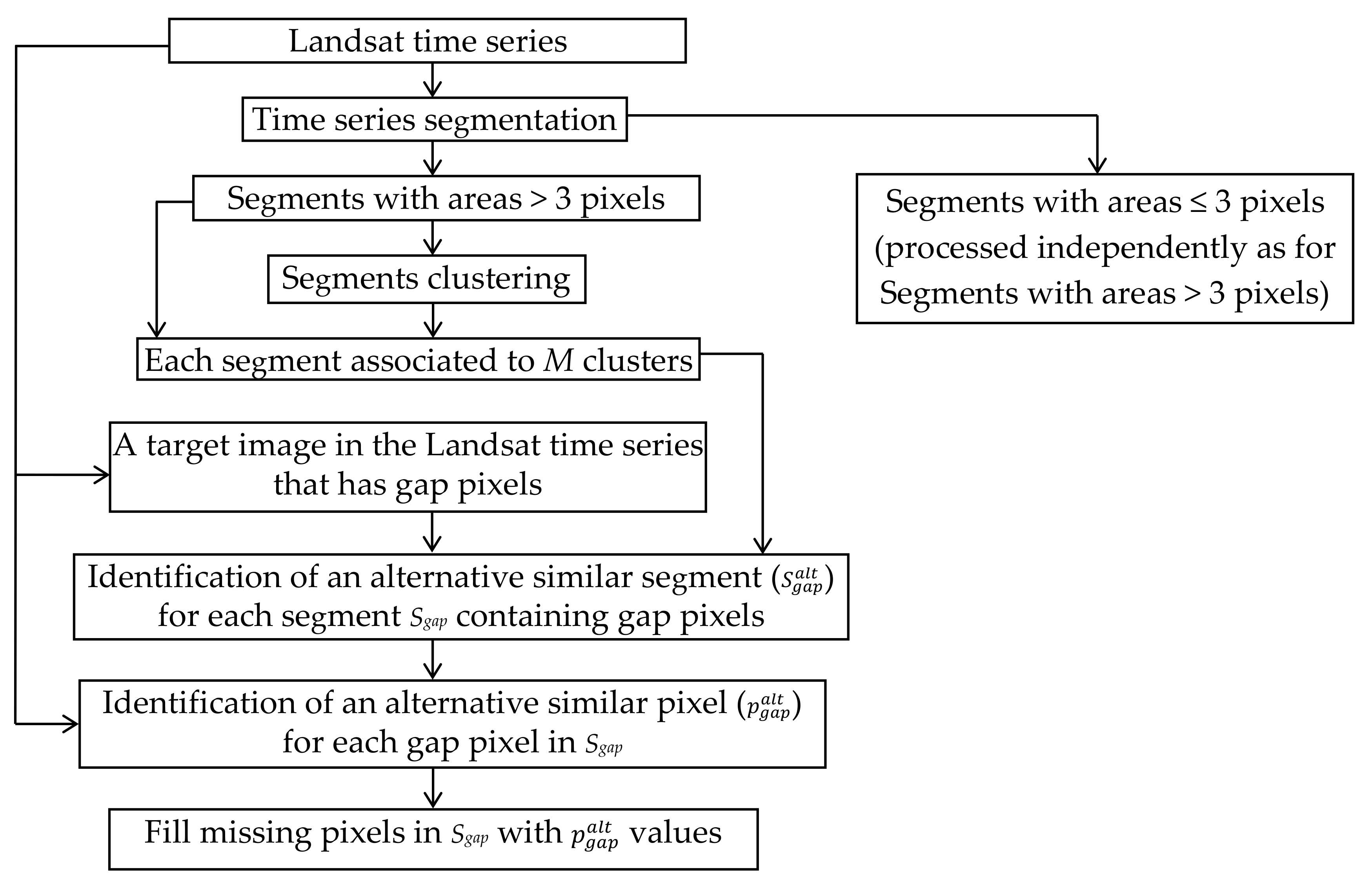
Figure 4.
Overview of the SAMSTS gap filling algorithm. (a) The segmentation map obtained from the time series; (b) The clustered segment (denoted by different hatching); (c) Given a segment with gaps (e.g., the red segment), its alternative segment is searched for considering only the segments in the same cluster (i.e., the purple, cyan and blue segments). The missing-observation-adaptive similarity metric SAMr is used in the segmentation, clustering, and alternative similar segment search.
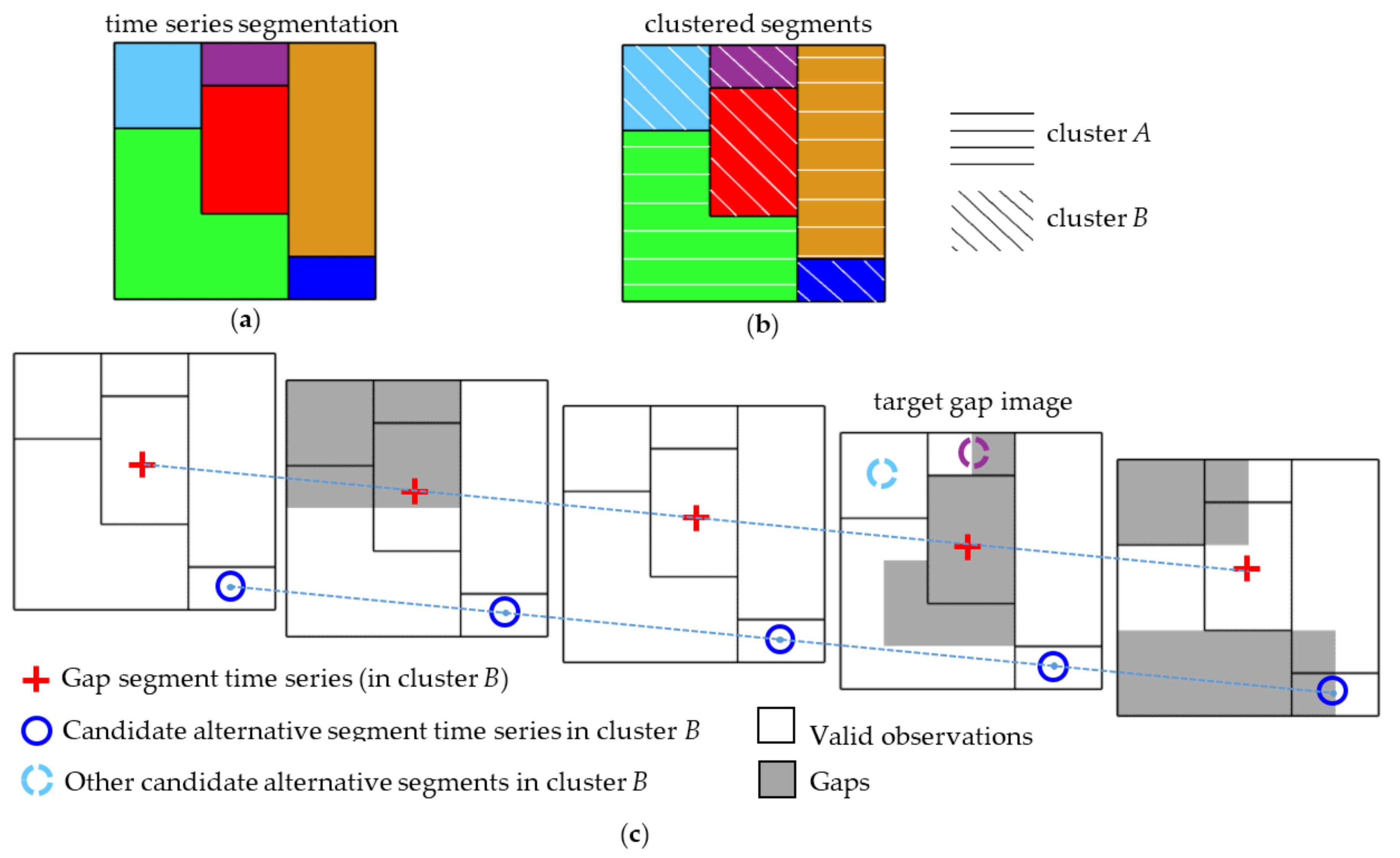
Figure 5.
Kansas 500 × 500 30 m pixel subset (centered at 37.75755020°N, 100.78698061°W, Figure 1c red square shows the subset tile location) results. 2010 CDL subset (a), Landsat 8 false-color (1.61 μm, 0.87 μm, 0.66 μm) images of the original (b), the preceding (d), and subsequent (f) weeks and the gap-filled version of the original data (e) and associated RMSD images (g–i) (colored: 0 ≤ dark blue ≤ 0.05; 0.05 < light blue ≤ 0.08; 0.08 < green ≤ 0.11; 0.11 < yellow ≤ 0.13; 0.13 < orange ≤ 0.15; 0.15 < red < 0.2; brown ≥ 0.2). The two red circles denote two circular center-pivot irrigation fields where partial harvesting occurred between weeks 36 and 38 and then complete harvesting occurred between weeks 38 and 40. The yellow arrow denotes a small area that was flooded between weeks 36 and 38.


Figure 6.
Example NDVI time series for the flooded pixel (denoted by the yellow arrows in Figure 5, located at 37.70121869°N, 100.82220237°W), and the corresponding NDVI time series for the selected alternative similar pixel. For clarity, the NDVI, rather than five-band reflectance time series, is shown.

Figure 7.
California tile (5000 × 5000 30 m pixels) gap filling experiments, 25 600 × 600 30 m pixel areas, shown by white squares in the target week (b), were removed to simulate gaps and then filled by the SAMSTS method (e), and by closest preceding (d) and subsequent (f) pixel substitution. Associated RMSD images are shown (g–i) colored as for Figure 5. The temporally-closest non-missing preceding and subsequent observations did not always belong to the same image and were acquired from one to five weeks before (a) and after (c) the target week, colored as black (1), dark gray (2), light gray (3), and white (4 or 5).
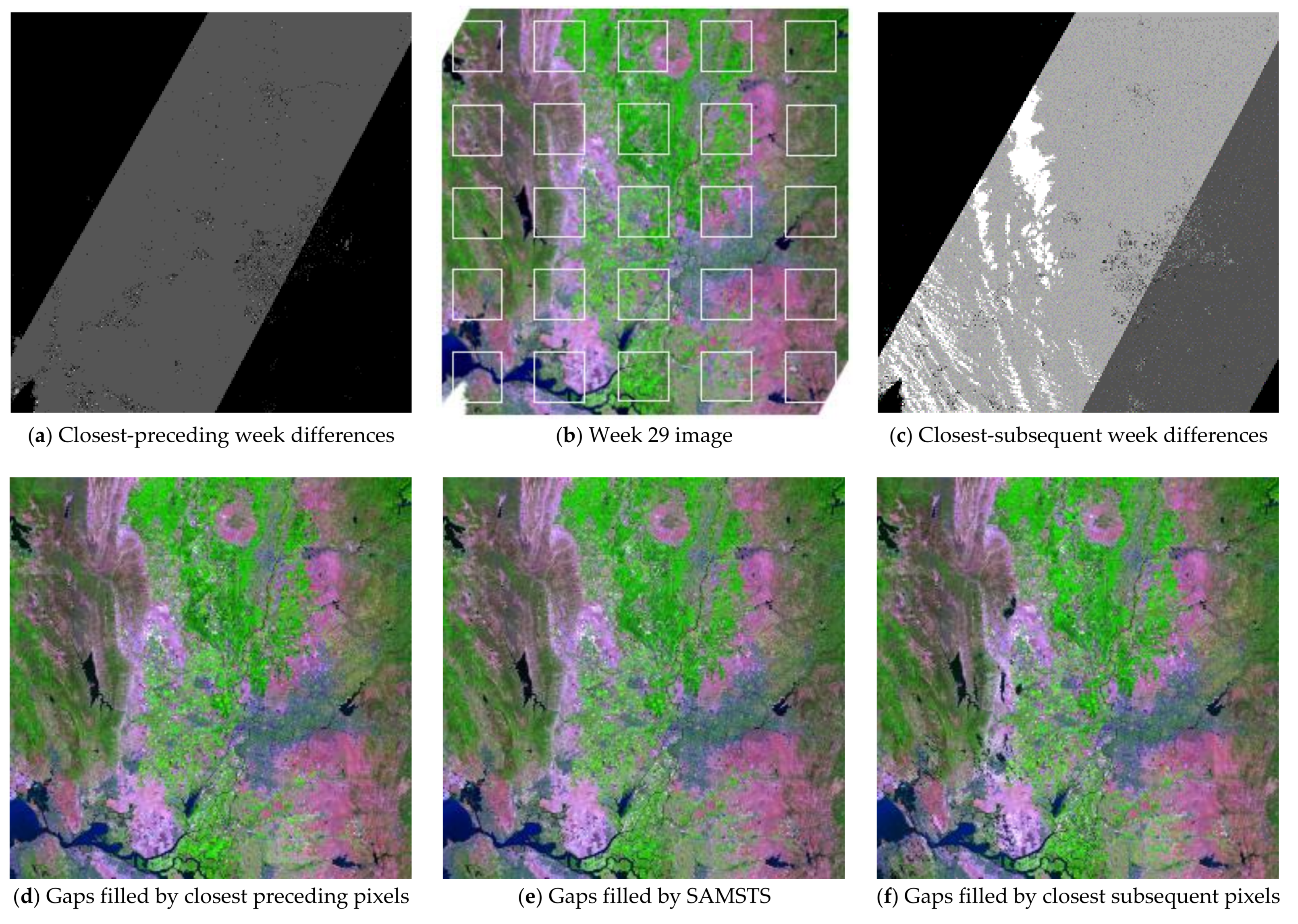

Figure 8.
Minnesota tile (5000 × 5000 30 m pixels) gap filling experiments, 25 600 × 600 30 m pixel areas, shown by white squares in the target week (b), were removed to simulate gaps and then filled by the SAMSTS method (e), and by closest preceding (d) and subsequent (f) pixel substitution. Associated RMSD images are shown (g–i) colored as for Figure 5. The temporally-closest non-missing preceding and subsequent observations did not always belong to the same image and were acquired from one to five weeks before (a) and after (c) the target week, colored as black (1), dark gray (2), light gray (3), and white (4 or 5).
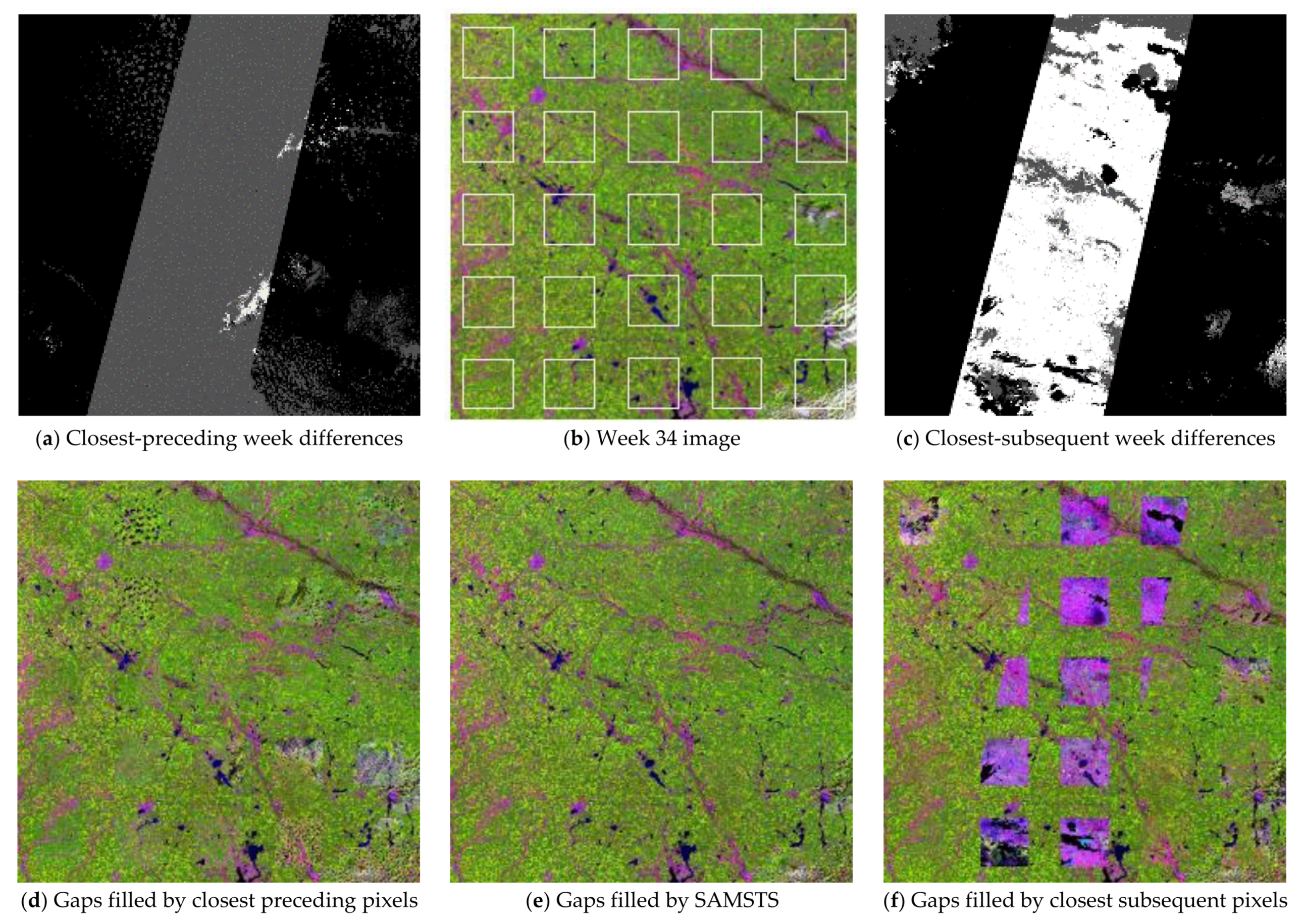

Figure 9.
Kansas tile (5000 × 5000 30 m pixels) gap filling experiments, 25 600 × 600 30 m pixel areas, shown by white squares in the target week (b), were removed to simulate gaps and then filled by the SAMSTS method (e), and by closest preceding (d) and subsequent (f) pixel substitution. Associated RMSD images are shown (g–i) colored as for Figure 5. The temporally-closest non-missing preceding and subsequent observations did not always belong to the same image and were acquired from one to five weeks before (a) and after (c) the target week, colored as black (1), dark gray (2), light gray (3), and white (4 or 5).
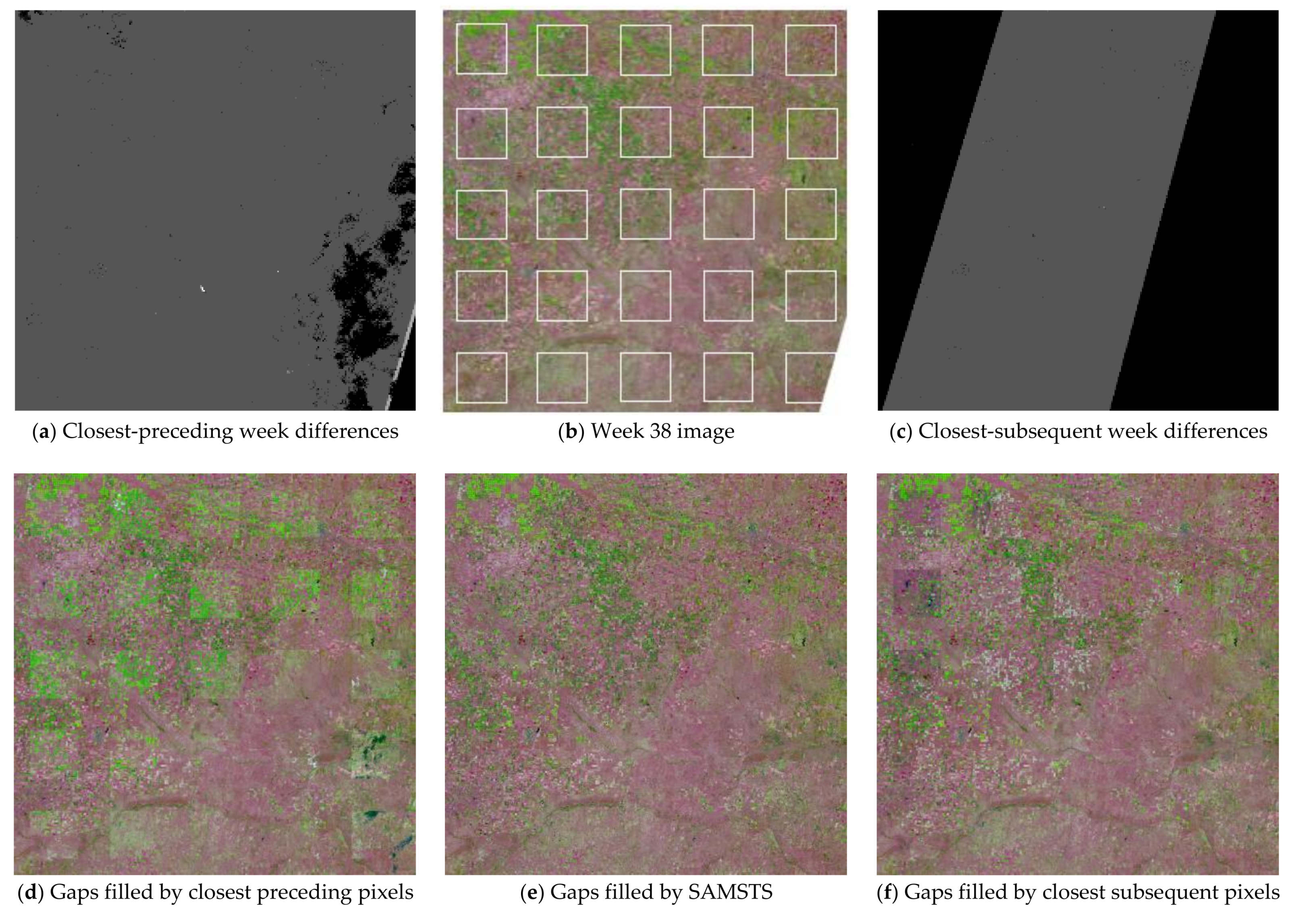

Figure 10.
Histograms of RMSDpreceding (red), RMSDsubsequent (green), RMSDtemporally_closest (black), and RMSDfill (blue) for the (a) California (Figure 7), (b) Minnesota (Figure 8) and (c) Kansas (Figure 9) tile results.

Figure 11.
Sinusoidal harmonic model gap-filling results for the 25 600 × 600 30 m pixel simulated gap areas for the California (a), Minnesota, (b) and Kansas (c) tiles. The original images before gap removal are illustrated in Figure 7b, Figure 8b, and Figure 9b. The associated RMSD gap-filling values are shown in (d–f) colored as for Figure 7, Figure 8 and Figure 9.


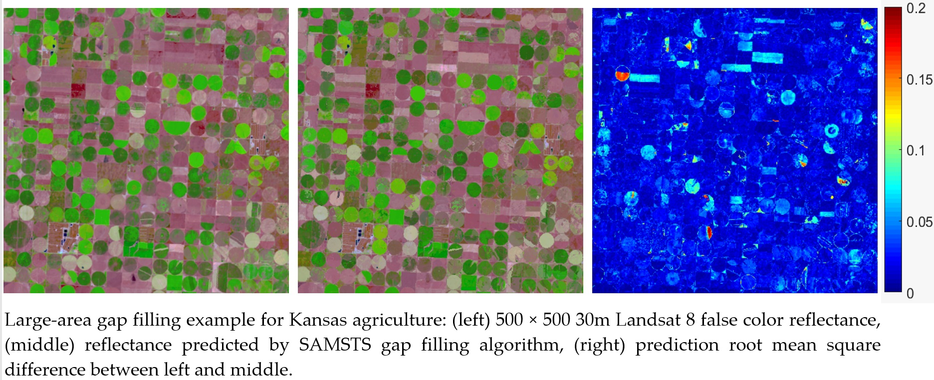
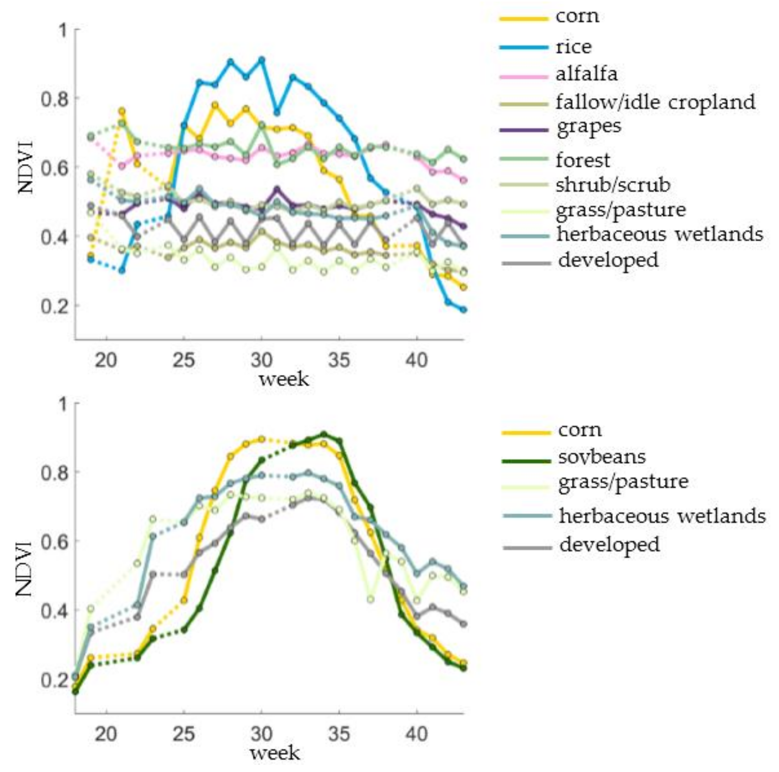
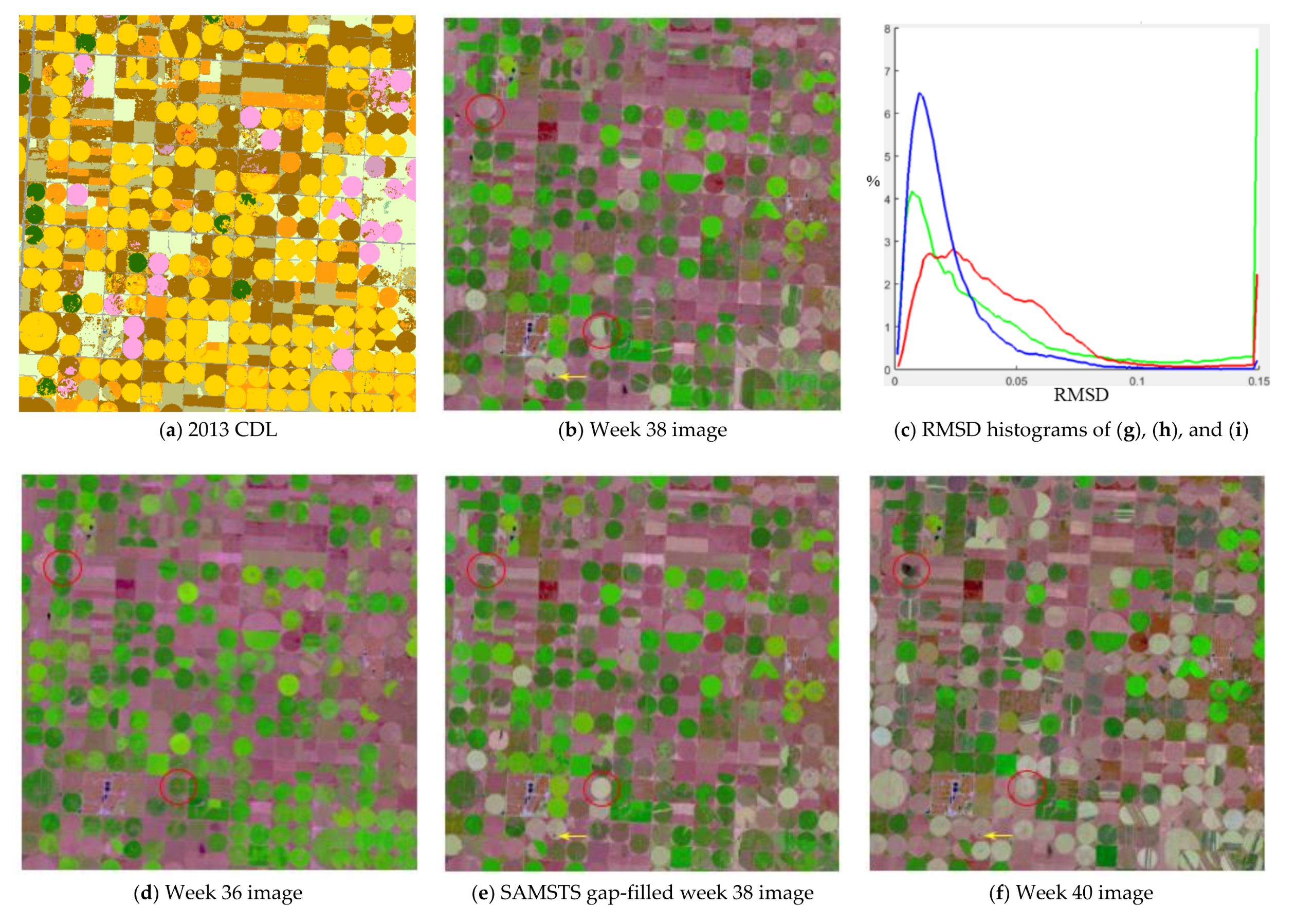
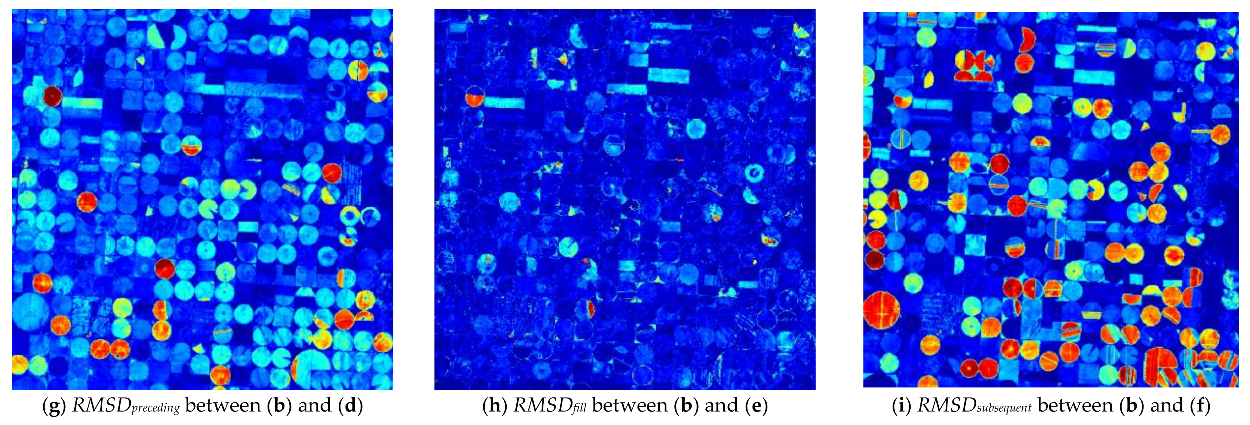
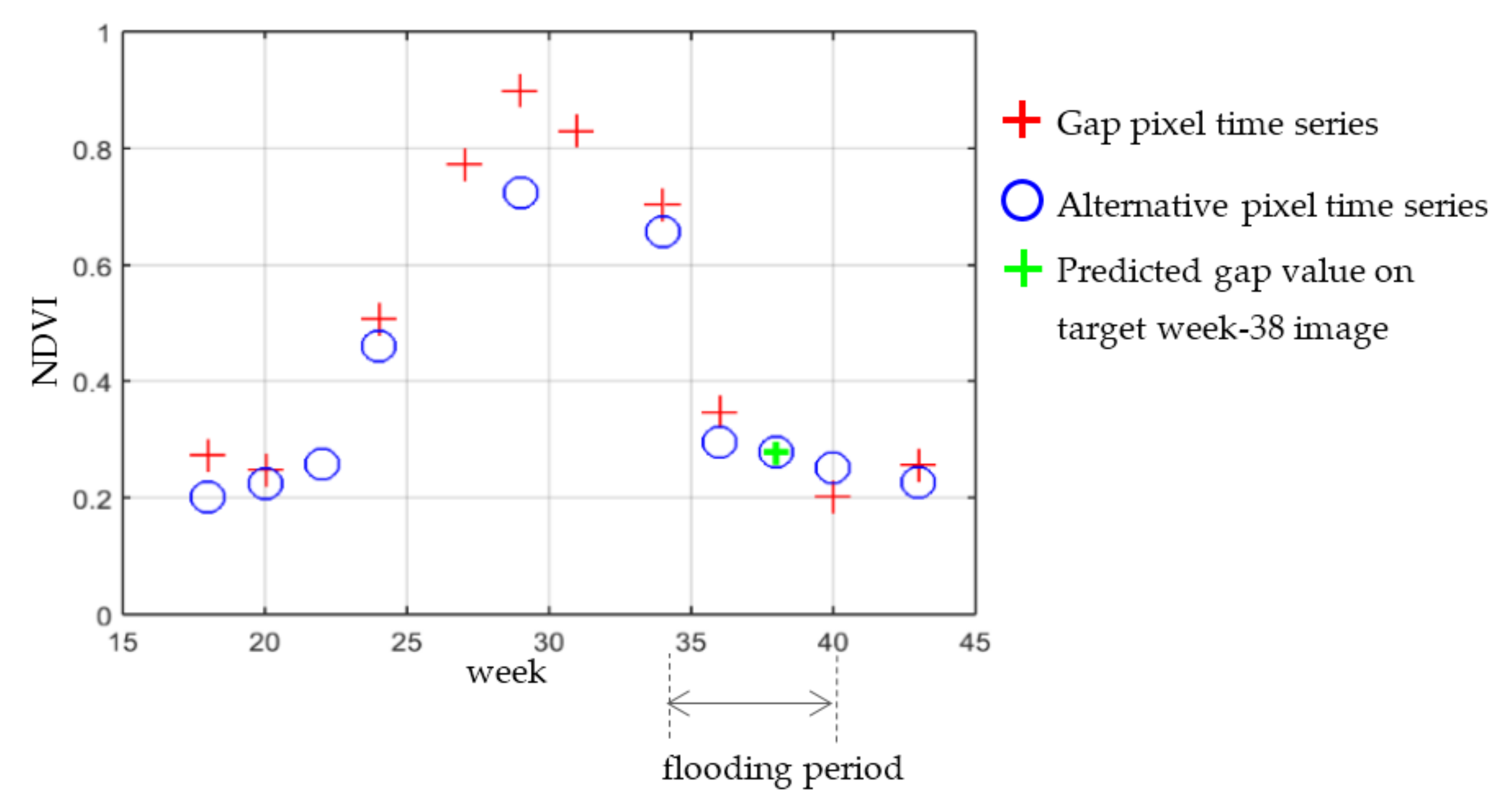
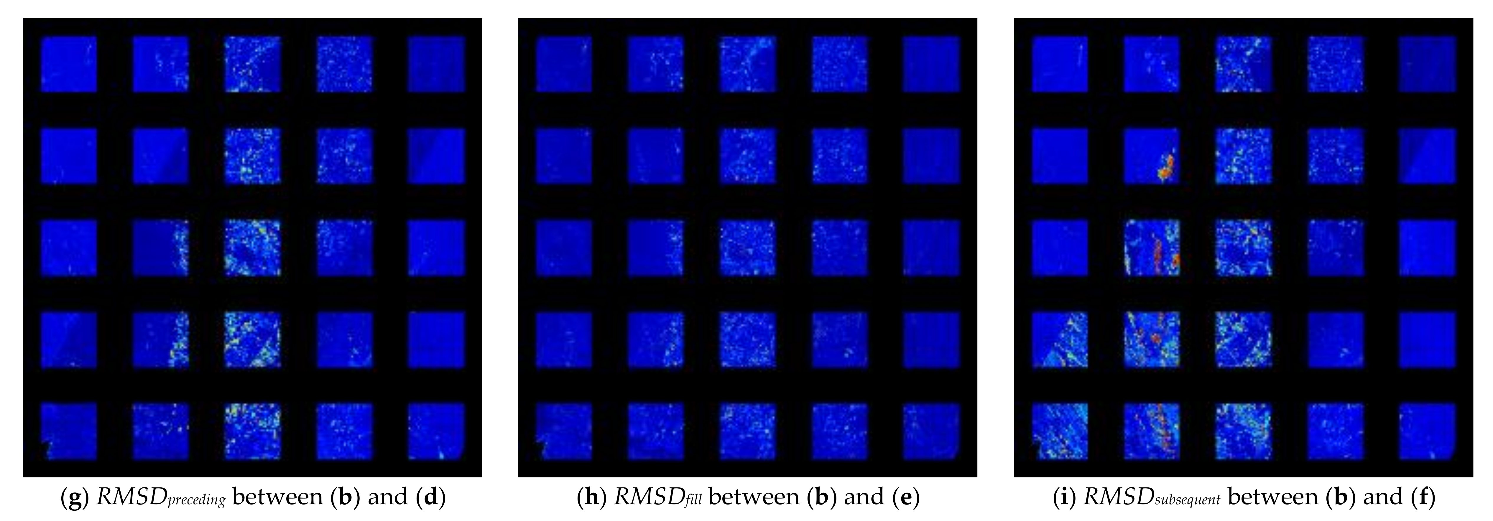
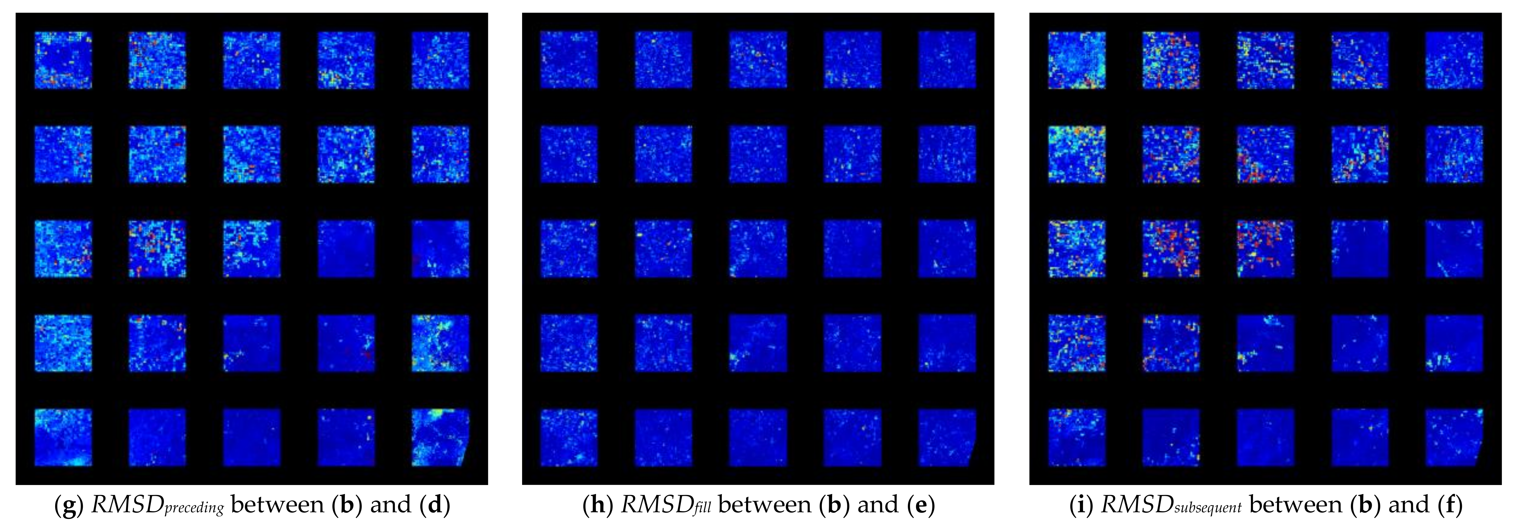
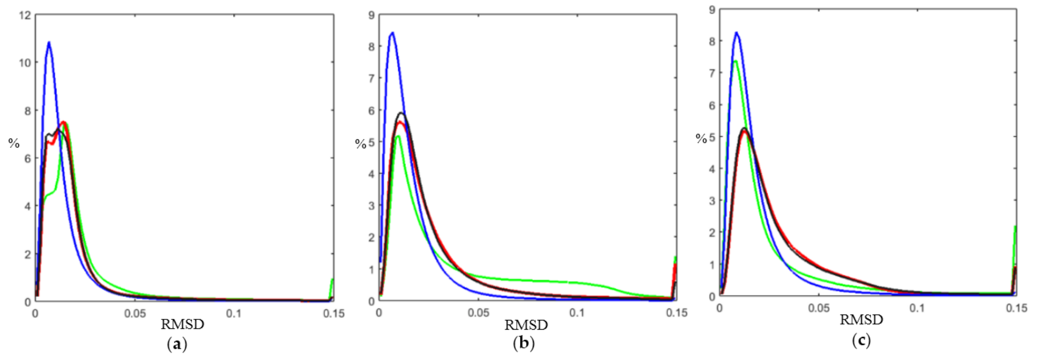
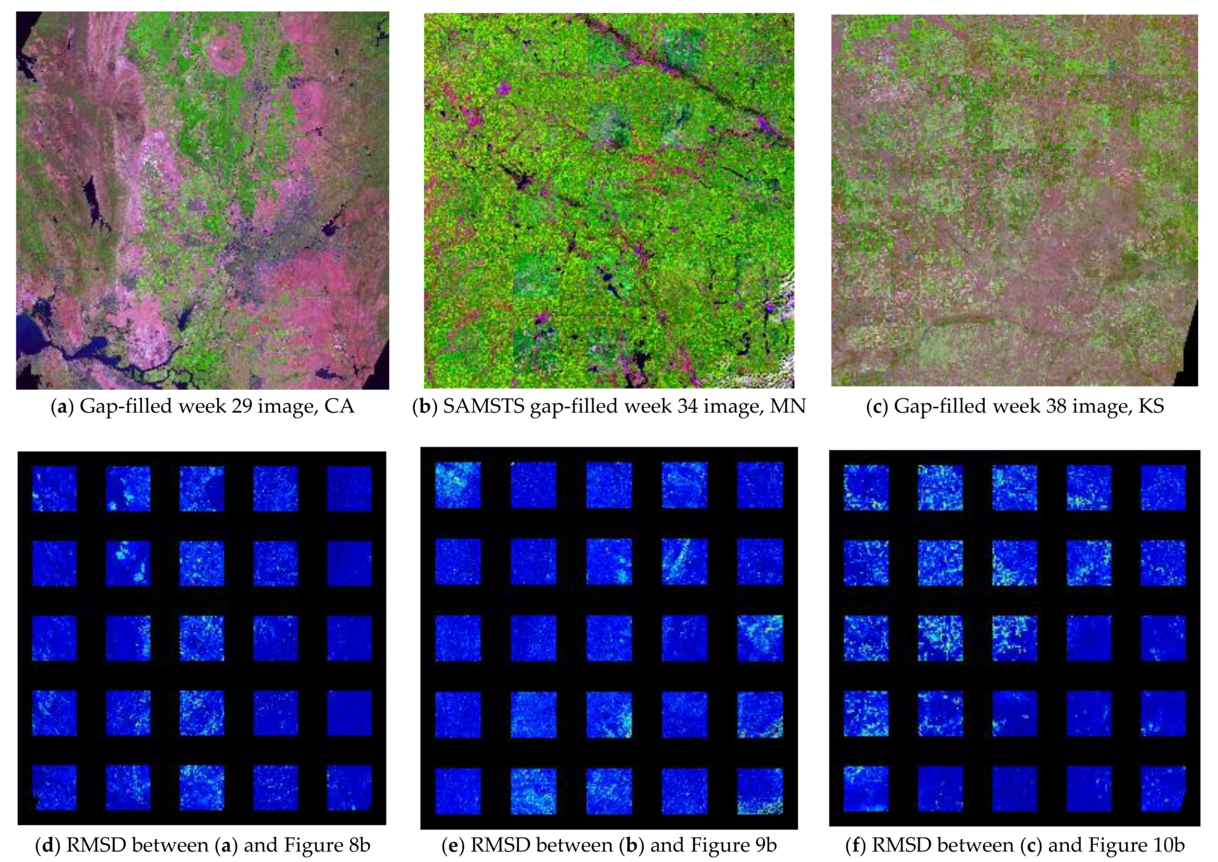
Table 1.
Summary of missing weekly pixel observations (26 weeks from 28 April to 26 October 2013) in the three test tiles. Note that in the same week different Landsat-8 orbits can overpass the eastern and western sides of a 5000 × 5000 30 m tile.
Table 1.
Summary of missing weekly pixel observations (26 weeks from 28 April to 26 October 2013) in the three test tiles. Note that in the same week different Landsat-8 orbits can overpass the eastern and western sides of a 5000 × 5000 30 m tile.
| Test Sites | Number of weeks (Out of 26) with at Least One Valid 30 m Pixel (n) in the Study Area | Percentage of Missing WELD Tile 30 m Pixel Observations over the 26 Weeks | Percentage of Missing Weekly WELD Tile 30 m Pixel Observations Computed over the n Weeks |
|---|---|---|---|
| California | 22 | 47.5% | 40.6% |
| Minnesota | 22 | 54.2% | 45.9% |
| Kansas | 20 | 46.2% | 30.1% |
Table 2.
Mean five-band RMSD values of the SAMSTS (Figure 7h, Figure 8h and Figure 9h) and the sinusoidal harmonic model gap-filling results (Figure 11d–f), with respect to all the pixels, the crop pixels, and the non-crop pixels as defined by the 2013 CDL (Figure 1).
| Test Sites | All (Crop and Non-Corp) | Crop | Non-Crop | |||
|---|---|---|---|---|---|---|
| SAMSTS | Harmonic | SAMSTS | Harmonic | SAMSTS | Harmonic | |
| California | 0.014 | 0.019 | 0.020 | 0.0300 | 0.012 | 0.016 |
| Minnesota | 0.016 | 0.025 | 0.015 | 0.026 | 0.018 | 0.021 |
| Kansas | 0.018 | 0.023 | 0.023 | 0.036 | 0.015 | 0.016 |
© 2018 by the authors. Licensee MDPI, Basel, Switzerland. This article is an open access article distributed under the terms and conditions of the Creative Commons Attribution (CC BY) license (http://creativecommons.org/licenses/by/4.0/).
Share and Cite
MDPI and ACS Style
Yan, L.; Roy, D.P. Large-Area Gap Filling of Landsat Reflectance Time Series by Spectral-Angle-Mapper Based Spatio-Temporal Similarity (SAMSTS). Remote Sens. 2018, 10, 609. https://doi.org/10.3390/rs10040609
AMA Style
Yan L, Roy DP. Large-Area Gap Filling of Landsat Reflectance Time Series by Spectral-Angle-Mapper Based Spatio-Temporal Similarity (SAMSTS). Remote Sensing. 2018; 10(4):609. https://doi.org/10.3390/rs10040609
Chicago/Turabian StyleYan, Lin, and David P. Roy. 2018. "Large-Area Gap Filling of Landsat Reflectance Time Series by Spectral-Angle-Mapper Based Spatio-Temporal Similarity (SAMSTS)" Remote Sensing 10, no. 4: 609. https://doi.org/10.3390/rs10040609
Note that from the first issue of 2016, this journal uses article numbers instead of page numbers. See further details here.