Diurnal Variation of Light Absorption in the Yellow River Estuary


1
School of Ecology and Environment, Inner Mongolia University, Hohhot 010021, China
2
First Institute of Oceanography, State Oceanic Administration, Qingdao 266061, China
3
Department of Biological and Agricultural Engineering, Texas A&M University, College Station, TX 77843, USA
4
Department of Civil and Environmental Engineering, Texas A&M University, College Station, TX 77843, USA
5
South China Institute of Environmental Sciences, the Ministry of Environmental Protection of RPC, Guangzhou 510301, China
*
Author to whom correspondence should be addressed.
Remote Sens. 2018, 10(4), 542; https://doi.org/10.3390/rs10040542
Submission received: 31 January 2018
/
Revised: 29 March 2018
/
Accepted: 29 March 2018
/
Published: 2 April 2018
(This article belongs to the Special Issue Remote Sensing of Short-Term Coastal Ocean Processes Enabled from Geostationary Vantage Point)
Abstract
:Considering the influence of river discharge and strong winds, the diurnal variability of ocean optical absorption properties in the Yellow River Estuary (YRE) is quantified, using in-situ measurements. The study finds that terrestrial sources due to the Yellow River discharge can cause high diurnal variation of water absorption because of the movement of river plume in the YRE, but such an influence diminishes far away from the Yellow River plume. The diurnal variability of water absorption, affected by strong winds, is found to be strengthened with a rapid increase of particles and colored dissolved organic matter (CDOM) arising from re-suspended sediment induced by wave forcing. The diurnal variability of particle absorption is controlled by non-algal particle absorption in the YRE, and the ratio of non-algal particle absorption (aNAP) and total particle absorption for most wavelengths is more than 0.56. The diurnal variation of spectral slope of non-algal particle absorption (SNAP) is found to vary within a narrow range, although large variability in the aNAP spectrum is observed. The CDOM is correlated negatively with salinity, and such negative correlation becomes weaker with the decreasing influence of riverine input. The spectral slope of CDOM absorption (Sg) may reflect the formation and constituents of CDOM with weak relationship to its concentration, and its relationship with the absorption of CDOM at 440 nm may be associated with the source of CDOM. The value of Sg, which is affected by re-suspended bottom sediment, is much lower than that derived from CDOM affected by Yellow River runoff. Disregarding the absorption of pure water, the diurnal variability of total water absorption stems principally from changes in non-algal particle matter rather than CDOM and Chl-a. By the observations of hourly GOCI (Geostationary Ocean Color Imager) data, the major diurnal variations of remote sensing reflectance at 680 nm are observed in near-coastal waters and the estuary of the Yellow River, which are mainly influenced by the flow discharge of Yellow River and strong winds. Finally, the seasonal differences of diurnal variations of water absorption caused by strong winds and river discharge are determined.
1. Introduction
Colored dissolved organic matter (CDOM), phytoplankton, and non-algal particles (NAP) are major light absorbing constituents in the ocean. These constituents determine the optical properties of natural waters and directly affect both the availability and spectral quality of light in the water column [1,2]. Through their effect on the submarine light field, these optically active constituents have a close relationship with biological activity. The changes in these constituents complicate remote sensing of Chl-a (chlorophyll-a concentration) and hence the estimation of primary product from ocean color imagery [3,4,5]. Therefore, a quantitative description of the dynamics and variability of water optical properties is especially important for better interpretation of satellite ocean color data and characterization of biogeochemical processes [6].
The optical properties for Case 1 waters, such as open oceanic waters, are relatively stable over large spatial and temporal scales due to the limited terrestrial and human influence. As opposed to Case 1 waters, the CDOM, phytoplankton, and non-algal particles for Case 2 waters are more abundant and variable due to the intricate hydrodynamic and ecological environment. Especially in the estuary waters, in addition to autogenic constituents which are composed of phytoplankton and its degradation products, large amounts of allogenic substances are transported from land by rivers or by wind, and substances are re-suspended from the sea bottom and are eroded from shorelines [7]. Moreover, non-algal particles and CDOM in the coastal regions and estuaries contribute significantly to the optical properties compared to phytoplankton, and the constituent concentrations may be uncorrelated with one another.
Although the optical properties of ocean color constituents have been studied in some coastal regions and estuaries, the diurnal variability of the optical properties of the natural waters is less well documented. Some studies have reported diurnal variability of particle backscattering, phytoplankton absorption [8,9], and ocean optical properties during a coastal algal bloom [6], based on in-situ observations.
The YRE receives a large influx of river runoff, mainly coming from the Yellow River which is the largest river that discharges into the Bohai Sea. The discharge of the Yellow River is a major source of freshwaters and supplies a dominant amount of terrestrial matters to the YRE. Therefore, the optical properties of the water body are complex and variable due to the mix of freshwater from the Yellow River discharge and saline sea water. Moreover, the YRE area is characterized by high suspended particle matter (SPM) concentration and complicated hydrodynamics, which poses a challenge for ocean color remote sensing [10,11,12,13,14]. However, the water optical properties in the YRE and its adjacent areas have been rarely reported [15], and the diurnal absorption variations of constituents and their mechanisms of influence on the environment have not been studied.
The objective of the present study therefore was to investigate the diurnal variations of light absorption by ocean constituents in the YRE, using in-situ continuous observation data. To understand the diurnal dynamics of CDOM and particle absorption, the influence of Yellow River discharge and strong winds on the diurnal absorption variability of these constituents was analyzed. Results of this study would improve our understanding of the YRE’s constituent abundance, spatial and temporal variability, and optical characteristics, and could provide some reference values for other large estuaries as well.
2. Data and Methods
2.1. Study Area
The YRE is located in the southwestern Bohai Sea, which is a semi-enclosed body of large, turbid and shallow water with an average depth of ~18 m in China [16]. Some regions of the YRE are very shallow, especially the coastal regions, but in general the turbidity of the waters limits the bottom effect in many instances and therefore does not contaminate ocean color imagery [17]. The Yellow River has an annual discharge of 420 × 108 m3 and an annual sediment load estimated at 109 tons, nearly accounting for more than half of the total river discharge to Bohai Sea [18]. The discharge of the Yellow River changes with season, and reaches a maximum in August and a minimum in April [19]. The tides are mainly semi-diurnal in the YRE, and the spatial variability of tidal amplitudes has been given by Hu et al. and Hainbucher et al. [20,21]. The basic hydrological features of the YRE, influenced by river inputs and dominated by runoff, can be summarized as low volume, heavy sands and weak tide [22]. This region is also characterized by complex and capricious optical properties due to the transport of huge amounts of inorganic sediments and organic matters by the Yellow River carrying to the sea.
2.2. Data Collection
Three continuous observations were conducted at 3 fixed stations in the YRE on 4 December 2011 (Station P1), 25 November 2011 (Station P2), and 11 December 2011 (Station P3), and the locations are shown in Figure 1. The average water depths at Stations P1, P2 and P3 are about 9.9 m, 16.5 m and 16.9 m, respectively. During the experiments, water samples were collected at the sea surface every hour from 8 a.m. to 9 a.m. the next day. Then, water samples were filtered and preserved immediately, and taken to the laboratory on shore to measure spectral absorption and biogeochemical properties. Salinity and temperature were measured with a CTD (Seabird, Seacat) during sampling.
2.2.1. Measurement of Suspended Particle Matter Concentration
The suspended particle matter concentration (SPM; units: mg/L) of the surface water was measured by a standard gravimetric method [23,24,25]. Water samples were collected from the top several centimeters of water surface using sampling bottles. The water samples were filtered through Whatman GF/F filters (Diameter 47 mm, pore size 0.45 mm). The filter was rinsed with 25–50 mL of pure water to remove as much salts as possible [26]. The weight of the filter paper had been measured in the laboratory before the cruise, and the filter paper was dried under infrared light and stored for on-shore analysis [17]. After taking to the laboratory, the filter was dried at 40 °C for 48 h and re-weighted at room temperature [27].
2.2.2. Measurement of Chlorophyll-a Concentration
For the estimation of total chlorophyll-a concentration (chl-a; units: μg/L), seawater samples (500 mL) were filtered through Whatman GF/F filter of 0.7 μm pore size under low vacuum pressure, and the filters were immediately preserved in liquid nitrogen before being processed. The filters were soaked in 90% acetone for 24 h and refrigerated in darkness at 4 °C in the laboratory. Then, Chlorophyll-a concentration (Chl-a) was determined for each sample using Turner-Design 10 fluorometer which was calibrated using Chl-a standards (Sigma, Sigma-Aldrich, St. Louis, MO, USA) [28].
2.2.3. Measurement of Light Absorption of Seawater
For the estimation of absorption coefficient of CDOM (ag(λ), units: m−1), seawater was filtered through polycarbonate filters of 0.22 μm pore size under low vacuum pressure. Absorbance spectra of CDOM were measured using a dual-beam Shimadzu spectrophotometer (UV-1800, Shimadzu, Japan) over the spectral range of 280 to 900 nm with an interval of 2 nm. Baseline data were obtained by filling Milli-Q water both in the sample and reference cells, and a baseline correction was applied by subtracting the offset from each sample spectrum [29].
For the estimation of absorption coefficient of particles (ap(λ), units: m−1) and non-algal particles (aNAP(λ), units: m−1), an adequate amount of seawater (depending on the particle load) was filtered through glass fiber filters of 0.7 μm pore size (Whatman GF/F) under low vacuum pressure. The absorption spectrum of the particles retained on the filter was measured for wavelengths between 280 and 900 nm with 2 nm increments using a dual-beam Shimadzu spectrophotometer (UV-1800) according to the filter-pad technique [30]. Non-algal spectral absorption was measured from the sample filter after bleaching of pigmented particles [31]. The background signals were subtracted, and correction of path-length described in Tassan et al. (2000) [32] was applied. The absorption coefficient for phytoplankton pigments (aph(λ), units: m−1) was then derived by subtracting aNAP(λ) from ap(λ).
2.2.4. Remote Sensing Reflectance
Inherent optical properties (IOPs) such as the absorption coefficient (a) and scattering coefficient (b), together with the directional structure of the ambient light field, determine the apparent optical properties (AOPs). As one of the important AOPs, the surface spectral reflectance derived from satellite sensors can be used to reflect the variation of absorption coefficient. To investigate the diurnal variability of water absorption in the larger area, the diurnal variation of remote sensing reflectance (Rrs) derived from GOCI (Geostationary Ocean Color Imager) images was analyzed.
The acquisition dates of the GOCI images with cloud-free or low cloud coverage were 22 September 2011, 16 October 2011, 25 October 2011 and 13 November 2011. The corresponding flow discharges of these days were 2670, 1150, 836 and 876 m3/s, respectively. According to the data of the National Center for Environmental Prediction (NCEP), strong winds began on 23 October, reached the highest speed of approximately 14.5 m/s at 6 p.m., and then gradually declined to 7.5 m/s on 25 October. The wind speed on 13 November was 9.81 m/s. Therefore, GOCI images (25 October and 13 November) can be used to map the spatio-temporal distributions of Rrs after strong winds, which could reveal the effect of strong winds on the diurnal variation of Rrs. Rrs(680) was selected as an indicator of SPM in the analysis below, due to its significant sensitivity to SPM variation in the turbid waters [22].
2.3. Data Analysis
The absorption by CDOM can be generally expressed by the following exponential equation [33]:
where ag(λ) and ag(λ0) represent the absorption of CDOM at any wavelength λ and a reference wavelength λ0, respectively. In general, the choice of a reference absorption wavelength is arbitrary, and several values of λ0 can be found in the literature [34]. However, 440 nm is generally chosen to be a reference wavelength because it corresponds, approximately, to the peak absorption by phytoplankton and represents the CDOM concentration, since CDOM is often measured optically at that wavelength [29,34]. Sg is the spectral slope coefficient obtained using a non-linear fit within a certain wavelength range, which means how rapidly the absorption decreases with increasing wavelength. In this paper, we chose the wavelength range from 380 to 690 nm. It must to be noted that the choice of representative wavelength range is different in most previous studies, which make the inter-comparison between various studies difficult [29,35,36,37].
Non-algal particles and CDOM often have similar spectral behavior, and have usually been modeled using the same exponential function as follows [38]:
where λ0 is the reference wavelength, aNAP(λ0) is the measured absorption value at the reference wavelength, and exponent SNAP represents the spectral slope of the absorption spectrum. In this study, the non-algal particle absorption spectrum fitted by the least square technique ranged from 380 to 700 nm, and 440 nm was chosen as the reference wavelength.
The descriptive statistics for the diurnal variations of water absorption was applied, that included the mean, maximum, and minimum values with standard deviations (SDs). The relationship of the parameters was indicated by means of the correlation coefficient (R). Based on the assumptions about independence, normal distribution and homogeneity of variances, one-way ANOVA (analysis of variance) was used to determine the difference or correlation, which defined statistically significant at p < 0.05. The ANOVA F test compares the variability between stations to the variability within stations. The number of degrees of freedom (DF) was the number of values in the calculation of a statistic.
3. Results
3.1. SPM and Chl-a Concentrations
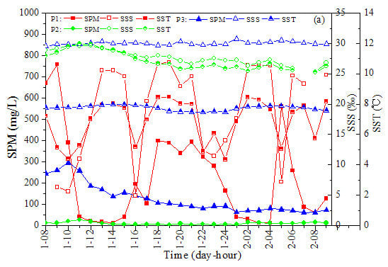
The hourly variation of SPM and Chl-a concentration for three fixed stations is shown in Figure 2. It is noted that patterns of variations of SPM and Chl-a concentration at the P1, P2 and P3 stations were different. For Station P1, the SPM concentration was found to vary significantly with fluctuations within 26 h. According to the statistics shown in Table 1, a maximum value of 758.69 mg/L was observed at 9 a.m. on day one and a much lower minimum value of 11.92 mg/L was observed at 4 a.m. the next day with the difference between them of 1 order of magnitude. At Station P2, with low SPM concentration less than 30 mg/L, the SPM diurnal variation of SPM was much smaller compared to Station P1, and the SD value of SPM was only 5.68 mg/L. At Station P3, the SPM concentration was always high during observation and decreased continuously from 10 a.m. on day one. However, the variations of Chl-a were not large for three stations with the measurement range from 0.24 to 1.34 μg/L, and the variation patterns of Chl-a and SPM were not alike.
Figure 2 also shows the variation of sea surface salinity (SSS) during observation at Stations P1, P2 and P3. The SSS of the P1 station was less than 27 psu with the lowest salinity of 4.92 psu, which was affected by the water from the Yellow River with low salinity and low temperature. Moreover, just as the variation of SPM, the SSS varied significantly with obvious fluctuation within 26 h, but the trend of change of SSS was opposite to that of SPM except for the time from 16 to 21 with relatively high SSS which could be caused by strong vertical mixing of the low and high salinity water. The dramatic variation of SSS at Station P1 indicates the influence of the Yellow River freshwater by river plume as time goes by. The SSS at Station P2 varied between 25.25 psu and 29.65 psu, which was higher compared to the Station P1. It is indicated that the influence of the Yellow River decreased for Station P2. For Station P3, the variation of SSS was small with the maximum and minimum values of 29.58 psu and 30.75 psu, respectively, which were close to the normal values of sea water. Furthermore, the correlation coefficient of SPM and SSS at Station P1 (R = −0.46; ANOVA: DF = 23, F = 5.92, p = 0.024) was larger than that at Stations P2 (R = 0.30, ANOVA: DF = 24, F = 2.28, p = 0.145) and P3 (R = −0.40, ANOVA: DF = 25, F = 4.69, p = 0.040). It is worth mentioning that the correlation coefficient of SPM and SSS for Station P1 reached −0.75 (DF = 23, F = 19.05, p < 0.001) if the data from local time 16 to 21 were removed.
Figure 3 shows the wind speed at YRE coming from NCEP in November and December 2011 and in-situ wind speed observed at Stations P1, P2 and P3 during the observation period. The wind speed at Station P3 was higher than that at Stations P1 and P2, the maximum wind speed was up to 10.4 m/s during the observation period. In addition, strong winds occurred on 7 and 10 December 2011 before observation, with the highest wind speed of approximately 14.2 m/s and 12.0 m/s, respectively.
In summary, we can conclude that Station P1 represents a typical estuarine environment which is affected by the Yellow River discharge, Station P2 is likely to have intermediate properties of both the marine and freshwater end members which are affected weakly by the Yellow River discharge, and Station P3 represents the marine environment which is affected by re-suspended sediment mainly induced by the earlier strong wind.
3.2. CDOM Absorption
3.2.1. Diurnal Variation of CDOM Absorption
Figure 4a shows the hourly spectral changes of CDOM absorption at Stations P1, P2 and P3. The diurnal variation of CDOM absorption was observed to have significant differences at Stations P1, P2 and P3. The hourly variations of absorption by CDOM at Station P1 and P3 were greater than that at Station P2. Figure 4b shows hourly variations of the CDOM absorption coefficient at 440 nm, large fluctuations of ag(440) were observed at the P1 and P3 stations. The statistics shown in Table 2 indicate that the difference of diurnal variation of ag(440) between Station P1 and Station P2 was significant (DF = 47, F = 16.29, p < 0.001) probably due to the different influence of terrigenous matter input from the Yellow River. The difference of diurnal variation of ag(440) between Station P3 and Station P2 was observed (DF = 48, F = 12.33, p < 0.001), which was attributed to the large variability of CDOM at Station P3 caused by re-suspended sediment induced by strong winds. It has been shown that strong winds can mix the shallow water column and release the CDOM trapped in sediments [39].
3.2.2. Relationship between CDOM Absorption and Salinity or Temperature
The sources of CDOM could be deduced with absorption coefficients and their correlation with environmental factors [40]. The relationship of ag(440) vs. SSS and SST (Sea Surface Temperature) for Stations P1, P2 and P3 is illustrated in Figure 5. A general trend of decreasing CDOM with increasing SSS and SST was observed at Station P1 with the correlation coefficient (R) of −0.49 (DF = 20, F = 5.91, p = 0.025) and −0.56 (DF = 21, F = 9.19, p = 0.007), and at Station P2 with the R of −0.52 (DF = 23, F = 8.13, p = 0.009) and −0.52 (DF = 23, F = 8.18, p = 0.009), but not observed at Station P3 with the R of 0.12 (DF = 24, F = 0.31, p = 0.583) and 0.01 (DF = 24, F = 0.002, p = 0.969). During observations at Stations P1 and P2, an overall larger range in salinity in comparison to Station P3 indicated a freshwater influence linked to the Yellow River discharge, which indicates that the Yellow River discharge is a significant factor controlling the variation of CDOM absorption, especially for Station P1 with the SSS range of 4.9 to 26.9 psu. The terrestrial input is the primary source of natural CDOM to the ocean in the YRE area, where the Yellow River runoff mixes with seawater. However, the weak correlation between ag(440) and SSS at P3 station suggests that it is not the Yellow River discharge but the bottom material re-suspension caused by strong winds that plays an important role in the variability of CDOM optical properties, just like causing the variation of SPM.
3.2.3. Spectral Slope of CDOM Absorption
In this paper, the CDOM absorption in the range of 380 to 690 nm was used to calculate Sg by exponential fitting with the correlation coefficient of more than 0.9, as the reference wavelength was set at 440 nm. The statistics of Sg are provided in Table 3. The Sg values at Station P1 and P2 have clear differences with the Sg values at Station P3. ANOVA tests indicated significant differences in Sg (DF = 46, F = 25.16, p < 0.001) between Stations P1 and P3, whereas no significant variability was observed in Sg (DF = 47, F = 2.73, p = 0.11) between Stations P1 and P2. Although the diurnal variation of Sg for each fixed station was found to be not as obvious as expected, it is apparent that the Sg value of CDOM at Station P3 showed a distinguishable pattern by contrast to Station P1 and P2. We can see that Sg which was affected by the re-suspended sediment was more variable and exhibited lower values than those derived from the CDOM affected by the Yellow River runoff. The variation of Sg was not greatly different between Stations P1 and P2 as the absorption of CDOM was. This showed that the variation of Sg could result from the change of composition, but not the concentration of CDOM [40]. The spectral slopes were not significantly different at Stations P1 and P2, likely indicating that similar CDOM sources were influenced by the Yellow River discharge in spite of the difference in the CDOM concentration, by contrast there was a bigger difference of Sg at Station P3 where the influence of wind was strong, which suggests a high degree of variability in the composition of CDOM in these waters. Therefore, even in the YRE, it is difficult to choose one Sg to represent the Sg of the whole study area because there are large differences in Sg which could be due to different sources of CDOM. This result demonstrates the potential for using Sg to characterize the composition of CDOM [41,42].
Some researchers found an inverse linear relationship between the logarithm of ag(440) and Sg [41]. In addition, according to [15], the absorption of CDOM at 440 nm and Sg can be parameterized using a power law, i.e.,
where Y0 and Y1 are undetermined coefficients. Figure 6 shows both kinds of relationship between Sg and ag(440) mentioned above. It can be seen that there is a strong negative relationship between ag(440) and Sg at Station P3 with the correlation coefficient greater than 0.92, and a weak negative relationship at Station P2 with the correlation coefficient higher than 0.24. However, the data from Station P1 do not exhibit the same behavior.
In Figure 6a,b, we can clearly identify two different CDOM sources which are from the terrestrial input and re-suspended sediments corresponding to Stations P1 and P3. These findings suggest that CDOM at Station P1 has different optical properties from those at Station P3, and this relationship between the spectral slope coefficient and absorption coefficient has potential to differentiate between terrestrially derived CDOM from marine source derived CDOM [34,43].
3.3. Particles Absorption
3.3.1. Total Particle Absorption
Figure 7 shows the spectral absorption coefficients for total particles (ap(λ)) and non-algal particles (aNAP(λ)) at Stations P1, P2 and P3. It can be seen that ap(λ) at Stations P1 and P3 were much higher than that at Station P2, which was accompanied by a greater diurnal variation. It is noted that the spectral absorption coefficient for total particles was nearly similar to that for non-algal particles, implying that the non-algal particles absorption could be the main contributor of ap(λ), which is different from that of open ocean water [44,45,46] and some eutrophic water [27], where the contribution of absorption by phytoplankton to the total particulate absorption is dominant.
Figure 8 shows the variation of non-algal particles to total particle absorption ratio aNAP(λ)/ap(λ) at different wavelengths as a function of the SPM concentration for Stations P1, P2 and P3. It shows that the contributions of aNAP(λ) to ap(λ) were more than 56.4% and 60.7% at all main wavelengths (these wavelengths corresponded to channels of the GOCI instrument) for Stations P1 and P3, respectively, while such contribution was relatively low at Station P2 with more than 56.3% for 412 nm, 443 nm, 490 nm and 555 nm, and more than 38.8% for 660 nm and 680 nm which was caused by the peak in phytoplankton absorption around 676 nm. It is noted that the aNAP(λ)/ap(λ) values are approximately the same as were observed in the Yangtze Estuary (especially inside the river’s mouth) [47], but significantly different from other areas. They were on average larger than those measured in the Mediterranean, Atlantic and subequatorial Pacific waters [46]. This suggests that, in the YRE waters, not only the amplitude of aNAP but also its relative contribution to total particle absorption was significantly different from that in other areas.
3.3.2. Non-Algal Particle Absorption
Figure 9 shows hourly variation of non-algal particle absorption coefficient at 440 nm; large fluctuations of aNAP(440) were observed at Station P1, relatively lower values of aNAP(440) were observed at Station P2, and a gradual decline of aNAP(440) was observed at Station P3. The statistics of non-algal particle absorption coefficients at 440 nm at different stations are shown in Table 4.
Figure 10 shows a relationship between aNAP(440) and SPM for Stations P1, P2 and P3. There was a positive relationship between aNAP(440) and SPM for Stations P1, P2 and P3 with a correlation coefficient R2 greater than 0.75, and this relationship can be described using a linear equation, as shown in Figure 10. It has been reported that organic particles may have a higher aNAP(443):SPM ratio than inorganic particles [38]. We can note that the slope at station 2 (0.045 m2g−1) was higher than that at Stations P1 and P3 (0.031 m2g−1 and 0.032 m2g−1) which also supported this interpretation. Figure 10 shows that the variation of aNAP(440) was actually in accordance with the variation of SPM with high values at Stations P1 and P3, low values at Station P2, which indicated that SPM was composed mainly of non-algal particles in the YRE.
The statistics of SNAP are shown in Table 5. The highest value and diurnal variation of SNAP were observed at Station P1, compared with the lowest value and diurnal variation of SNAP at Station P3. ANOVA tests indicated that some differences of SNAP seemed to occur between different stations (P1–P2: DF = 37, F = 17.29, p < 0.001; P1–P3: DF = 33, F = 63.66, p < 0.001; P2–P3: DF = 39, F = 18.83, p < 0.001), but the resulting SNAP values were within the range of values found in other regions given by Babin et al. [38].
3.4. Total Water Absorption
Defining the total absorption in a water column as the sum of absorption by pure water (aw), phytoplankton (aph), non-algal particles (aNAP), and CDOM (ag), the total absorption coefficient (at) at wavelength λ, can be expressed as [38,48,49,50]:
The relative contribution of a given component was calculated as the ratio of the absorption coefficient of that component to the total absorption coefficient of non-water constituents. Figure 11 illustrates the relative contribution of absorption by non-algal particles, phytoplankton pigments and CDOM derived from our data as triangular diagrams at six different wavelengths. As can be seen, the total absorption of non-water constituents in all our samples was almost dominated by non-algal particles at all wavelengths, except for only a few samples at Station P2 at longer wavelengths (660 nm and 680 nm) due to the absorption of phytoplankton. At all main wavelengths, the average contributions of non-algal particles (aNAP) to the total non-water absorption (aph + aNAP + ag) were 75.3 ± 11.5%, 63.2 ± 11.6% and 76.5 ± 10.3% for Stations P1, P2 and P3, respectively. Only a small percentage of light in the estuary was absorbed by phytoplankton and CDOM, the spectrally averaged percentages for each material were: phytoplankton, 17.7 ± 9.7% (P1), 19.5 ± 8.3% (P2) and 18.0 ± 7.3% (P3), CDOM, 7.0 ± 6.2% (P1), 17.3 ± 9.0% (P2) and 5.5 ± 5.0% (P3). It is noted that the contributions of CDOM to the total absorption were less than 29.0% for P1, 46.7% for P2 and 21.9% P3. This result is different from the previous reports which indicated CDOM can contribute more than 50% to the light absorption budget at short wavelengths (e.g., 440 nm) at the surface of the ocean [14,38,46]. It is also noted that the variations of the contributions of different components to the total absorption were related to the wavelength; with decreasing wavelength, the contributions of non-algal particles and CDOM increased. On the contrary, the contribution of phytoplankton was becoming the important absorber at the red end of the spectrum (660 nm and 680 nm), especially for Station P2.
Disregarding the absorption due to pure water, we found that the total non-water absorption was dominated by the particle absorption at almost all wavelengths, especially at Stations P1 and P3. Therefore, these results suggested that the water in the YRE was a typical Case 2 water, where non-algal particles were the dominant component affecting optical properties, and that the diurnal variability of absorption by water was principally due to non-algal particle matter rather than CDOM and Chl-a [11,42].
3.5. Diurnal Variation of Remote Sensing Reflectance
Figure 12 shows the diurnal variation of Rrs at different GOCI bands at Stations P1, P2 and P3 in four different days. It shows that the magnitude of diurnal variation of Rrs at Station P1 was larger than that at Stations P2 and P3 for all four days. According to the statistics shown in Table 6, the SDs in different days at Station P1 were the largest compared to those at Stations P2 and P3, and the values of SD were consistent with the flow discharges of Yellow River, with the maximum and minimum SDs occurring on 22 September and 13 November. The SDs at Station P2 were larger than the SDs at Station P3 due to the different distances to the Yellow River mouth. In addition, it was found that the SDs at Stations P1 and P2 on 25 October and 13 November were larger than they were on 22 September and 16 October, which could be related with the re-suspension of SPM caused by strong winds.
As shown in Figure 13, using the GOCI 500-m data, we obtained hourly maps of Rrs(680) in the YRE and its adjacent areas (including Bohai Bay and Laizhou Bay) on four different days. By the observations of hourly GOCI, the Rrs(680) diurnal variations can be seen in the study area on these days. The SD images show that different regions exhibited different magnitudes of diurnal variations. The major regions of Rrs(680) diurnal variation were generally located in near-coastal waters and in the estuary of the Yellow River. The diurnal variations of Rrs(680) in the Bohai Bay and Laizhou Bay were higher than those in the center of Bohai Sea. With the effect of previous strong winds, the SDs of Rrs(680) on 25 October and 13 November increased over a broad region, especially in the Bohai Bay and Laizhou Bay.
Therefore, we can conclude that the flow discharge of Yellow River and strong winds have a significant impact on the diurnal variation of Rrs in the YRE and its adjacent areas, which is consistent with the results of the light absorption study based on in-situ experimental investigation.
4. Discussion
4.1. Diurnal Variation of Light Absorption
4.1.1. CDOM Absorption
Based on the observations at the P1 and P2 stations, it can be concluded that the diurnal variation of CDOM absorption decreased from the river estuary toward the offshore area. Meanwhile, observations at Station P3 show that the diurnal variation of CDOM absorption has a significant increase resulting from the re-suspended sediment. Considering the effect of river runoff and strong wind, the values of ag(440) found for Yellow River Estuary in this study were basically in the range observed for Bohai Sea by Zhou et al. [15], who reported that the range of ag(440) in the Bohai Sea was from 0.0958 to 0.7795 m−1, and average value of ag(440) was 0.2311 m−1.
CDOM usually has a much higher concentration in estuaries than in other marine systems [51], and most of it is introduced into the estuary by the way of river discharge. Generally, the component of CDOM is influenced by terrigenous sediment for the estuarine and coastal waters, and by marine sediment for the offshore waters. The high diurnal variation of CODM absorption at Station P1 was caused by terrigenous sediment that came with the Yellow River discharge, while this influence was reduced far away from the Yellow River plume at Station P2, where the variation of absorption of CODM was influenced by terrigenous sediment together with marine sediment.
In fact, the CDOM absorption shows a linear inverse correlation with salinity in many estuarine and coastal waters [5,52,53,54,55,56,57], and based on this finding salinity fields are tracked through remote sensing-based observation of CDOM [10,57,58]. Previous observations discovered that the negative relationship between SSS and ag(440) would begin to loosen as the SSS reached a certain extent, indicating a decreased influence of riverine input of CDOM [5,37,59]. The present study demonstrates that this type of slope discontinuity breaks down at Station P3 with salinity more than 29.6 psu.
Previous studies in the Bohai Sea showed that the average value of Sg derived for the wavelength range of 380–550 nm was 0.015 nm−1 and its standard deviation was 0.0039 nm−1 [15], which was similar to the average value of Sg at all the three stations, but with a greater SD value due to the large study area. It also can be found that the Sg values at Stations P1 and P2 except for Station P3 were nearly similar to the range of (0.013–0.018 nm−1) reported by Blough and Del Vecchio (2002) [53] for coastal waters influenced by river input and were close to the commonly assumed value of (0.015 nm−1) for CDOM in coastal waters [38].
Zhou et al. (2015) [15] reported that weak negative correlations between Sg and ag(440) were observed in the Bohai Sea and Northern Yellow Sea based on 895 stations surveyed during China’s offshore marine optical investigation, but there was no clear relationship between Sg and ag(440) in most of the Chinese offshore waters [15]. In addition, this inverse relationship between the CDOM absorption at a certain wavelength and Sg has been reported before in the literature [34,41,43,60,61,62,63], whereas such a relationship was not found by other research reports [15,38,41,56]. It is indicated that this negative relationship between Sg and ag(440) can be associated with the source of CDOM, which was discussed by Xing et al. (2008) [64].
4.1.2. Particles Absorption
Although a large variability in the aNAP spectrum was observed in this study, the spectral slope SNAP varied within a narrow range which meant that the overall spectral shape was rather conservative for three stations. The low SNAP approaching 0.011 nm−1 was found for mineral particles in the North Sea [38] and Irish Sea [65], meanwhile the high SNAP approaching 0.013 nm−1 was observed in the Baltic Sea which is known for its high organic matter content [38]. The range of SNAP values derived at all three stations was relatively narrow, with the mean SNAP less than 0.0113 nm−1 close to that found for mineral particles. Moreover, no obvious difference was observed for SNAP when comparing Station P1 and Station P3, and its average (0.0113 nm−1 and 0.0103 nm−1) was similar to the average found for mineral particles by Bowers et al. (1996) [65] and Ferreira et al. (2014) [56]. In addition, the generally narrow range of variation in SNAP restricts this parameter used for purposes of monitoring [56], but allows a reliable modeling of aNAP due to the lack of dependence on the variables.
4.1.3. Total Water Absorption
The high variation of total absorption coefficient in a water column was caused by the variable contributions of the components other than pure water [11,38,45,66]. The variability of absorption coefficient in open-ocean waters (Case 1 waters) has been well studied, and it has been reported that open ocean samples were dominated by phytoplankton absorption and all components except pure water are often assumed to covary with Chl-a concentration [11,44,45,46,48,67]. In contrast, the variability of absorption coefficient in coastal, estuarine and inland waters (Case 2 waters) were relatively poorly documented, and the components were considered to vary widely and independently (IOCCG, 2000). Moreover, the non-algal particles and CDOM make significant contributions to the total absorption in coastal and estuarine waters in addition to phytoplankton [38,56].
4.2. Factors Affecting Light Absorption Diurnal Variation
The YRE, well-known for its high SPM concentration in the world, is one of the most significant eco-regions that can be easily affected by its complicated hydrodynamic environment. In general, hydrological factors, which can cause a complicated water environment in and outside the estuary, mainly include river discharge, tidal currents, and wave forcing induced by wind [22,68,69,70,71,72,73].
4.2.1. Strong Winds
As already analyzed for Station P3, under the strong wind influence, the water absorption experienced large variations within 26 h, especially with a rapid increase of particles and CDOM coming from re-suspended sediments, which cause the bio-optical properties much more complex. However, it has been reported that such a sharp increase, induced by re-suspended sediments at the sea surface, was episodic, had a short duration, and returned to normal quickly after the passage of a strong wind, which was also evidenced by satellite-retrieved data [22,72,74] and in-situ buoy data [74], respectively. However, the wind speed varies strongly with season, associated closely with monsoon activity in the study area. East Asian Monsoon has been considered to be a significant driving force for spatial and temporal sediment distribution in coastal waters [73,75,76,77,78]. The northerly winds in the winter are stronger than the dominant southerly winds in the summer, as is characteristic for the Bohai Sea. The events of maximum wind speed greater than 11 m/s from the northwest and northeast often occurred in the winter season [79]. The submarine sediments are frequently re-suspended and transported by storm waves which are closely associated with the prevailing winds in the winter season [73,80,81,82,83,84,85,86]. Therefore, considering the shallow nature, climate and adequate terrestrial sediment supply from major rivers in the study area, winds in the winter season must play a major role in the diurnal variation of absorption by waters, resulting in significant seasonal differences of diurnal variations in water absorption.
4.2.2. Yellow River Discharge
The diurnal variation of water absorption in the YRE was affected by terrigenous matter that came with the Yellow River discharge, although this influence declined with the increase of distance from Yellow River plume. The degree of influence of terrigenous matter could be related with the river flow. In general, the water and sediment discharges of the Yellow River into the sea have a significant seasonal variability. Figure 14 shows the daily average discharge and sediment concentration of the Yellow River which were observed at the Lijin hydrological gauging station (obtained from the website http://www.mwr.gov.cn/) in 2011. In natural conditions, the flow discharge was larger in the wet season with high sediment concentration than in the dry season. However, apart from natural causes, the water and sediment discharges of Yellow River have been regulated since 2000 by the operation of the Xiaolangdi Reservoir, the largest reservoir in the mainstream, through the Project of “Artificial Regulation of the Yellow River Water and Sediment” [87]. Thus, the flow discharge distribution had two high peaks from late June to early July and from late September to early October, respectively, which was due to reservoir’s flood relief in the Yellow River upstream. Hence, the diurnal variation of water absorption in different seasons will definitely vary with the change of flow discharge and sediment concentration. Furthermore, considering the seasonal variation of monsoon, the strong wind could expand the influence of river discharge on the diurnal variation of water absorption at temporal and spatial scales.
4.2.3. Tidal Cycle
Aside from the strong wind-induced re-suspended sediment which caused the diurnal variation of water absorption, the tidal cycle may enhance vertical mixing and bottom sediment re-suspension, and thus can systematically and sustainably increase the variation of water absorption and change an area optically [56,72,74,88,89,90]. Cheng et al. (2016) [72] reported that macro-tidal currents play a significant role in the diurnal variation of suspended particle matter in the Yalu River Estuary of China, and there were usually two peaks of suspended particle matter in a tidal cycle corresponding to the maximum flood and ebb current. In addition, in Hangzhou Bay, He et al. (2013) [74] revealed that tide was the main driver of the diurnal spatial and temporal variability using in-situ data and GOCI-derived suspended particle matter concentration. Ferreira et al. (2014) [56] reported that strong tidal variations played a role in the distribution of suspended material and the relative contribution of organic and inorganic components in Santos Bay.
It is important to note that the various regions and tidal phases have different magnitudes of diurnal variations, which, to a great extent, could be dependent on water depth and tidal range. In general, the tidal cycle variations of re-suspended sediment often occur in the coastal region due to shallow water, while the tidal effect on the diurnal variation of re-suspended sediment is insignificant and even negligible in the open ocean [89]. It has been demonstrated that the re-suspended sediment in the water column is correlated with the integration of tidal currents as well as the water depth in some studies [88,89,91,92]. In addition, the magnitude of tide current was strongly correlated with the temporal and spatial variation of tidal range. A large magnitude of tidal current can induce a strong bottom shear stress and enhance stronger re-suspension of sediment, which could cause a high variation of water constituents in the coastal water [74]. In contrast, a small tidal current with weak bottom shear stress and sediment re-suspension had limited influence on the variation of water constituents. With regard to the YRE area, the tide regime is complex and dominated by irregular semi-diurnal tides with an average tidal range of 0.6–0.8 m, and that increases both southward and northward reaching 1.5–2.0 m at Bohai Bay and Laizhou Bay [85,86,93]. Therefore, we can conclude that tidal cycle is one of the hydrodynamic factors that can drive the diurnal variation of water absorption in the coastal region with shallow water of the YRE. However, this effect of tidal cycle on the diurnal variation of water absorption could be weak in the study area by comparison with macro-tidal estuary and coasts. In addition to tidal cycle, the current circulation was considered as the key hydrodynamic factor controlling the sediment distribution and transport in the region [85], so it may be a reasonable reason for elevated SPM and the factor affecting the light absorption diurnal variation to consider.
4.3. Implications of Diurnal Variation for Remote Sensing Products
The complex optical properties of Case 2 waters present distinct challenges to bio-optical modeling and remote sensing retrieval algorithms. In general, local empirical inversion algorithms were developed for the Case 2 water to solve its applicability problem caused by the temporal and spatial variation of optical properties. Our results indicate that bio-optical parameters could have significant diurnal variability caused by the hydrological and climatic factors. These short-term changes of optical properties challenge the applicability of local empirical inversion algorithms. To further improve the performance of ocean color inversion algorithms, the effect of temporal IOP variability needs to be fully considered [6,94,95].
The validation of remote sensing products relies on a high-quality match-up dataset between satellite and in-situ data. It is difficult to perform measurements that are ideally synchronous with satellite overpass at specific sites for the majority of in-situ–satellite match-ups, so time differences are unavoidable in most cases. It was reported that a time window (e.g., 1–3 h) is usually accepted as a compromise [17,96,97,98]. According to our result, the errors induced by a 3 h time difference between in-situ measurements and satellite overpass could be great in certain areas or under certain climate conditions. Therefore, significant uncertainties introduced by time window due to the temporal variability and the effect of the relaxed match-up criterion on the assessment result should be considered in the validation activities, especially for the regions or conditions with significant diurnal variations.
In addition, our results indicated that short-term processes, such as the diurnal variation of IOPs caused by flow discharge of the River and strong winds, often occurred in the estuarine and coastal waters. Since the traditional polar-orbiting ocean color satellites may be insufficient to detect/monitor short-term processes for areas of significant temporal variability, the geostationary ocean color satellite with high-spatial and high-spectral resolution measurements would play a significant role in helping monitor short term and regional oceanic phenomena.
5. Conclusions
The diurnal variability of ocean optical absorption properties in the YRE is quantified, using in-situ measurements. The diurnal variation of absorption by water constituents, including CDOM and particles, can be affected by river discharge and wave forcing induced by strong winds. Terrestrial sources through the Yellow River discharge can cause a high diurnal variation of water absorption by the movement of river plume in the YRE. However, such an influence declines far away from the Yellow River plume. The diurnal variability of water absorption during a strong wind is found to be strengthened with a rapid increase of CDOM and particles coming from the re-suspended sediment induced by wave forcing.
We observe a general trend of decreasing ag(440) with increasing SSS in the YRE. However, such a negative relationship between CDOM and salinity begins to weaken as the SSS reaches a certain extent, which indicates a decreasing influence of riverine input of CDOM. It is demonstrated that Sg could reflect the formation and component of CDOM, with weak relationship with the CDOM concentration. The diurnal variation of Sg at one fixed station is found to be as not obvious as expected. However, considering the different sources of CDOM, Sg which is affected by re-suspended sediment, is more variable and exhibits much lower values than those derived from CDOM affected by the Yellow River runoff. Consistent with previous studies, there exist an unstable negative relationship between Sg and ag(440), which could be associated with the source of CDOM.
Different from the situation of open ocean waters and some eutrophic waters, the variability in particle absorption s controlled by non-algal particle absorption in the YRE, and the ratio of aNAP(λ)/ap(λ) at most wavelengths, except for 660 nm and 680 nm, is more than 56.4%. There was a positive relationship between aNAP(440) and SPM in the study area, which indicates that SPM was composed mainly of non-algal particles in the YRE. The diurnal variation of SNAP at all three stations is found to vary within a narrow range, although large variability in the aNAP spectrum is observed.
Disregarding the absorption of pure water, the total non-water absorption is dominated by the non-algal particle absorption at almost all wavelengths in the YRE, which suggests that the diurnal variability of water absorption is principally due to non-algal particle matter rather than CDOM and Chl-a.
By the observations of hourly GOCI, it is seen that the major regions of Rrs(680) diurnal variation are generally located in near-coastal waters and in the estuary of the Yellow River. The flow discharge of the Yellow River and strong winds have a significant impact on the diurnal variation of Rrs in the YRE and its adjacent areas, which is consistent with the results of the light absorption study based on in-situ experimental investigation.
Finally, we discuss the seasonal differences of diurnal variations in water absorption caused by strong wind and river discharge in the study area. Considering the characteristics of monsoon activities, frequent winds in the winter season must play a major role in the diurnal variation of water absorption. The diurnal variation of water absorption in different seasons varies with the change of flow discharge and sediment concentration in the area close to the river plume. In addition, the tidal cycle can increase the diurnal variation of water absorption by enhancing vertical mixing and bottom sediment re-suspension in the shallow coastal water.
Acknowledgments
This work was funded by the National Key Research and Development Program of China (2016YFA0600102), the National Natural Science Foundation of China (61461034, 51469018, 61265008, 41506202, and 41476159), Inner Mongolian Natural Science Foundation of China (2014BS0605), Public Science and Technology Research Funds Projects of Ocean of China (2013418025-2), and the China–Korea Joint Ocean Research Center (PI-2017-3).
Author Contributions
Yanling Hao prepared data, analyzed and interpreted the data and results, and wrote the manuscript; Tingwei Cui collected in-situ data, analyzed data and contributed to the discussions; Vijay P. Singh and Jie Zhang contributed to the discussions and suggestions to improve the quality of manuscript; Ruihong Yu reviewed the manuscript, and added some interpretations of results; and Wenjing Zhao contributed to the collection and processing of in-situ data.
Conflicts of Interest
The authors declare no conflict of interest.
References
- Vecchio, R.D.; Blough, N.V. Influence of ultraviolet radiation on the chromophoric dissolved organic matter in natural waters. In Environmental UV Radiation: Impact on Ecosystems and Human Health and Predictive Models, Proceedings of the NATO Advanced Study Institute, Pisa, Italy, 30 April–10 May 2001; Ghetti, F., Checcucci, G., Bornman, J.F., Eds.; NATO Science Series: IV; Earth and Environmental Sciences; Springer: Berlin, Germany, 2006; Volume 57. [Google Scholar]
- Hargreaves, B.R. Water column optics and penetration of UVR. In UV Effects in Aquatic Organisms and Ecosystems; Helbling, E.W., Zagarese, H., Eds.; The Royal Society of Chemistry: Cambridge, UK, 2003; Volume 1, pp. 59–108. [Google Scholar]
- Antoine, D.; André, J.M.; Morel, A. Oceanic primary production: II. Estimation at global scale from satellite (Coastal Zone Color Scanner) chlorophyll. Glob. Biogeochem. Cycles 1996, 10, 57–69. [Google Scholar] [CrossRef]
- Behrenfeld, M.J.; Falkowski, P.G. Photosynthetic rates derived from satellite based chlorophyll concentrations. Limnol. Oceanogr. 1997, 42, 1–20. [Google Scholar] [CrossRef]
- Xie, H.; Aubry, C.; Bélanger, S.; Song, G. The dynamics of absorption coefficients of CDOM and particles in the St. Lawrence estuarine system: Biogeochemical and physical implications. Mar. Chem. 2012, 128, 44–56. [Google Scholar] [CrossRef]
- Cui, T.W.; Cao, W.X.; Zhang, J.; Hao, Y.; Yu, Y.; Zu, T.T.; Wang, D.X. Diurnal variability of ocean optical properties during a coastal algal bloom: Implications for ocean colour remote sensing. Int. J. Remote Sens. 2013, 34, 8301–8318. [Google Scholar] [CrossRef]
- Woźniak, S.B.; Meler, J.; Lednicka, B.; Zdun, A.; Stoń-Egiert, J. Inherent optical properties of suspended particulate matter in the southern Baltic Sea. Oceanologia 2011, 53, 691–729. [Google Scholar]
- Mercado, J.M.; Ramírez, T.; Cortés, D.; Sebastián, M. Diurnal changes in the bio-optical properties of the phytoplankton in the Alborán Sea (Mediterranean Sea). Estuar. Coast. Shelf Sci. 2006, 69, 459–470. [Google Scholar] [CrossRef]
- Ohi, N.; Saito, H.; Taguchi, S. Diel patterns in chlorophyll a specific absorption coefficient and absorption efficiency factor of picoplankton. J. Oceanogr. 2005, 61, 379–388. [Google Scholar] [CrossRef]
- Bowers, D.; Evans, D.; Thomas, D.; Ellis, K.; Williams, P.J.L.B. Interpreting the colour of an estuary. Estuar. Coast. Shelf Sci. 2004, 59, 13–20. [Google Scholar] [CrossRef]
- Morel, A.; Prieur, L. Analysis of variations in ocean color. Limnol. Oceanogr. 1977, 22, 709–722. [Google Scholar] [CrossRef]
- D’Sa, E.J.; Ko, D.S. Short-term influences on suspended particulate matter distribution in the northern Gulf of Mexico: Satellite and model observations. Sensors 2008, 8, 4249–4264. [Google Scholar] [CrossRef] [PubMed]
- D’Sa, E.J.; Miller, R.L.; Del Castillo, C. Bio-optical properties and ocean color algorithms for coastal waters influenced by the Mississippi River during a cold front. Appl. Opt. 2006, 45, 7410–7428. [Google Scholar] [CrossRef] [PubMed]
- Siegel, D.A.; Maritorena, S.; Nelson, N.B.; Hansell, D.A.; Lorenzi-Kayser, M. Global distribution and dynamics of colored dissolved and detrital organic materials. J. Geophys. Res. Ocean. 2002, 107. [Google Scholar] [CrossRef]
- Zhou, H.L.; Zhu, J.H.; Li, T.J. Spectral properties of colored dissolved organic matter in Chinese offshore waters. J. Trop. Oceanogr. 2015, 34, 23–29, (In Chinese with English Abstract). [Google Scholar]
- Ruddick, K.; Vanhellemont, Q.; Yan, J.; Neukermans, G.; Wei, G. Variability of suspended particulate matter in the Bohai Sea from the geostationary Ocean Color Imager (GOCI). Ocean Sci. J. 2012, 47, 331–345. [Google Scholar] [CrossRef]
- Cui, T.; Zhang, J.; Groom, S.; Sun, L.; Smyth, T.; Sathyendranath, S. Validation of MERIS ocean-color products in the Bohai Sea: A case study for turbid coastal waters. Remote Sens. Environ. 2010, 114, 2326–2336. [Google Scholar] [CrossRef]
- Wei, H.; Sun, J.; Moll, A.; Zhao, L. Phytoplankton dynamics in the Bohai Sea-observations and modelling. J. Mar. Syst. 2004, 44, 233–251. [Google Scholar] [CrossRef]
- Wang, Q.; Guo, X.; Takeoka, H. Seasonal variations of the Yellow River plume in the Bohai Sea: A model study. J. Geophys. Res. 2008, 113, C08046. [Google Scholar] [CrossRef]
- Hu, F.; Gu, G. Seasonal changes of the mean tidal range along the Chinese coasts. Oceanol. Limnol. Sin. 1989, 20, 401–411. [Google Scholar]
- Hainbucher, D.; Hao, W.; Pohlmann, T.; Feng, S.; Suendermann, J. Variability of the Bohai Sea circulation based on model calculations. J. Mar. Syst. 2004, 44, 153–174. [Google Scholar] [CrossRef]
- Zhao, W.; Sun, L.; Cui, T.; Cao, W.; Ma, Y.; Hao, Y. Mapping the distribution of suspended particulate matter concentrations influenced by storm surge in the Yellow River Estuary using FY-3A MERSI 250-m data. Aquat. Ecosyst. Health 2014, 17, 290–298. [Google Scholar] [CrossRef]
- Zhang, M.; Tang, J.; Dong, Q.; Song, Q.; Ding, J. Retrieval of total suspended matter concentration in the Yellow and East China Seas from MODIS imagery. Remote Sens. Environ. 2010, 114, 392–403. [Google Scholar] [CrossRef]
- Choi, J.K.; Park, Y.J.; Ahn, J.H.; Lim, H.S.; Eom, J.; Ryu, J.H. GOCI, the world’s first geostationary ocean color observation satellite, for the monitoring of temporal variability in coastal water turbidity. J. Geophys. Res. 2012, 117, C09004. [Google Scholar] [CrossRef]
- Min, J.E.; Ryu, J.H.; Lee, S.; Son, S. Monitoring of suspended sediment variation using Landsat and MODIS in the Saemangeum coastal area of Korea. Mar. Pollut. Bull. 2012, 64, 382–390. [Google Scholar] [CrossRef] [PubMed]
- Van der Linde, D.W. Protocol for Determination of Total Suspended Matter in Oceans and Coastal Zones; Technical Note I.98.182; Joint Research Centre: Brussels, Belgium, 1998. [Google Scholar]
- Wang, G.; Cao, W.; Yang, Y.; Zhou, W.; Liu, S.; Yang, D. Variations in light absorption properties during a phytoplankton bloom in the Pearl River estuary. Cont. Shelf Res. 2010, 30, 1085–1094. [Google Scholar] [CrossRef]
- Parsons, T.R.; Maita, Y.; Lalli, C.M. A Manual of Chemical and Biological Methods for Seawater Analysis; Pergamon Press: Oxford, UK, 1984. [Google Scholar]
- Nima, C.; Frette, Ø.; Hamre, B.; Erga, S.R.; Chen, Y. Absorption properties of high-latitude Norwegian coastal water: The impact of CDOM and particulate matter. Estuar. Coast. Shelf Sci. 2016, 178, 158–167. [Google Scholar] [CrossRef]
- Mitchell, B.G.; Kahru, M.; Wieland, J.; Stramska, S. Determination of spectral absorption coefficients of particles, dissolved material and phytoplankton for discrete water samples. In Ocean Optics Protocols for Satellite Ocean Colour Sensor Validation; Mueller, J.L., Fargoin, G.S., McClain, C.R., Eds.; Revision 4, NASA/TM-2003-211621/Rev4-vol.4; NASA Goddard Space Flight Center: Greenbelt, MD, USA, 2003; Volume IV (Chapter 4), pp. 39–64. [Google Scholar]
- Tilstone, G.H.; Moore, G.F.; Sørensen, K.; Doerfeer, R.; Røttgers, R.; Ruddick, K.D.; Pasterkamp, R.; Jørgensen, P.V. Regional Validation of MERIS Chlorophyll Products in North Sea Coastal Waters; REVAMP Methodologies EVGI-CT-2001-00049; VRIJE Universiteit Amsterdam: Amsterdam, The Netherlands, 2001. [Google Scholar]
- Tassan, S.; Ferrari, G.M.; Bricaud, A.; Babin, M. Variability of the amplification factor of light absorption by filter-retained aquatic particles in the coastal environment. J. Plankton Res. 2000, 22, 659–668. [Google Scholar] [CrossRef]
- Bricaud, A.; Morel, A.; Prieur, L. Absorption by dissolved organic matter of the sea (yellow substance) in the UV and visible domains. Limnol. Oceanogr. 1981, 26, 43–53. [Google Scholar] [CrossRef]
- Stedmon, C.A.; Markager, S.; Kaas, H. Optical properties and signatures of chrompophoric dissolved organic matter (CDOM) in Danish waters. Estuar. Coast. Shelf Sci. 2000, 51, 267–278. [Google Scholar] [CrossRef]
- Blough, N.V.; Del Vecchio, R. Chromophoric DOM in the coastal environment. In Biogeochemistry of Marine Dissolved Organic Matter; Hansell, D.A., Carlson, C.A., Eds.; Academic Press: San Diego, CA, USA, 2002; pp. 509–578. [Google Scholar]
- Twardowski, M.S.; Boss, E.; Sullivan, J.M.; Donaghay, P.L. Modeling the spectral shape of absorption by chromophoric dissolved organic matter. Mar. Chem. 2004, 89, 69–88. [Google Scholar] [CrossRef]
- Granskog, M.A.; Macdonald, R.W.; Mundy, C.-J.; Barber, D.G. Distribution, characteristics and potential impacts of chromophoric dissolved organic matter (CDOM) in Hudson Strait and Hudson Bay, Canada. Cont. Shelf Res. 2007, 27, 2032–2050. [Google Scholar] [CrossRef]
- Babin, M.; Stramski, D.; Ferrari, G.M.; Claustre, H.; Bricaud, A.; Obolenski, G.; Hoepffner, N. Variations in the light absorption coefficients of phytoplankton, nonalgal particles, and dissolved organic matter in coastal waters around Europe. J. Geophys. Res. 2003, 108. [Google Scholar] [CrossRef]
- Joshi, I.; D’Sa, E.J. Seasonal Variation of Colored Dissolved Organic Matter in Barataria Bay, Louisiana, Using Combined Landsat and Field Data. Remote Sens. 2015, 7, 12478–12502. [Google Scholar] [CrossRef]
- Zhang, X.Y.; Chen, X.; Deng, H.; Du, Y.; Jin, H.Y. Absorption features of chromophoric dissolved organic matter (CDOM) and tracing implication for dissolved organic carbon (DOC) in Changjiang Estuary, China. Biogeosci. Discuss. 2013, 10, 12217–12250. [Google Scholar] [CrossRef]
- Matsuoka, A.; Bricaud, A.; Benner, R.; Para, J.; Sempéré, R. Tracing the transport of colored dissolved organic matter in water masses of the Southern Beaufort Sea: Relationship with hydrographic characteristics. Biogeosci. Discusss. 2012, 9, 925–940. [Google Scholar] [CrossRef]
- Hong, H.; Wu, J.; Shang, S.; Hu, C. Absorption and fluorescence of chromophoric dissolved organic matter in the Pearl River Estuary, South China. Mar. Chem. 2005, 97, 78–89. [Google Scholar] [CrossRef]
- Kowalczuk, P.; Stoń-Egiert, J.; Cooper, W.J.; Whitehead, R.F.; Durako, M.J. Characterization of chromophoric dissolved organic matter (CDOM) in the Baltic Sea by excitation emission matrix fluorescence spectroscopy. Mar. Chem. 2005, 96, 273–292. [Google Scholar] [CrossRef]
- Cleveland, J.S. Regional models for phytoplankton absorption as a function of chlorophyll a concentration. J. Geophys. Res. 1995, 100, 13333–13344. [Google Scholar] [CrossRef]
- Bricaud, A.; Morel, A.; Babin, M.; Allali, K.; Claustre, H. Variations of light absorption by suspended particles with chlorophyll a concentration in oceanic (case 1) waters: Analysis and implications for bio-optical models. J. Geophys. Res. 1998, 103, 31033–31044. [Google Scholar] [CrossRef]
- Bricaud, A.; Babin, M.; Claustre, H.; Ras, J.; Tièche, F. Light absorption properties and absorption budget of Southeast Pacific waters. J. Geophys. Res. 2010, 115, C08009. [Google Scholar] [CrossRef]
- Shen, F.; Zhou, Y.; Hong, G. Absorption property of non-algal particles and contribution to total light absorption in optically complex waters, a case study in Yangtze Estuary and adjacent coast. Adv. Comput. Environ. Sci. 2012, 142, 61–66. [Google Scholar]
- Prieur, L.; Sathyendranath, S. An optical classification of coastal and oceanic waters based on the specific spectral absorption curves of phytoplankton pigments, dissolved organic matter, and other particulate materials. Limnol. Oceanogr. 1981, 26, 671–689. [Google Scholar] [CrossRef]
- Roesler, C.S.; Perry, M.J.; Carder, K.L. Modeling in situ phytoplankton absorption from total absorption spectra in productive inland marine waters. Limnol. Oceanogr. 1989, 34, 1510–1523. [Google Scholar] [CrossRef]
- Carder, K.L.; Hawes, S.K.; Baker, K.A.; Smith, R.C.; Steward, R.G.; Mitchell, B.G. Reflectance model for quantifying chlorohyll a in the presence of productivity degradation products. J. Geophys. Res. 1991, 96, 20599–20611. [Google Scholar] [CrossRef]
- Kirk, J.T.O. Light and Photosynthesis in Aquatic Ecosystems, 2nd ed.; Cambridge University Press: Cambridge, MD, USA, 1994. [Google Scholar]
- Monahan, E.C.; Pybus, M.J. Colour, ultraviolet absorbance and salinity of the surface waters off the west coast of Ireland. Nature 1978, 274, 782–784. [Google Scholar] [CrossRef]
- McKee, D.; Cunningham, A.; Jones, K. Simultaneous measurements of fluorescence and beam attenuation: Instrument characterisation and interpretation of signals from strati-fied coastal waters. Estuar. Coast. Shelf Sci. 1999, 48, 51–58. [Google Scholar] [CrossRef]
- Bowers, D.G.; Harker, G.E.L.; Smith, P.S.D.; Tett, P. Optical properties of a region of freshwater influence (the Clyde Sea). Estuar. Coast. Shelf Sci. 1999, 50, 717–726. [Google Scholar] [CrossRef]
- Bélanger, S.; Xie, H.; Krotkov, N.; Larouche, P.L.; Vincent, W.F.; Babin, M. Photomineralization of terrigenous dissolved organic matter in Arctic coastal waters from 1979 to 2003, Interannual variability and implications of climate change. Glob. Biogeochem. Cycles 2006, 20, GB4005. [Google Scholar] [CrossRef]
- Ferreira, A.; Ciotti, Á.M.; Coló Giannini, M.F. Variability in the light absorption coefficients of phytoplankton, nonalgal particles, and colored dissolved organic matter in a subtropical bay (Brazil). Estuar. Coast. Shelf Sci. 2014, 139, 127–136. [Google Scholar] [CrossRef] [Green Version]
- Bowers, D.G.; Brett, H.L. The relationship between CDOM and salinity in estuaries: An analytical and graphical solution. J. Mar. Syst. 2008, 73, 1–7. [Google Scholar] [CrossRef]
- Sasaki, H.; Siswanto, E.; Nishiuchi, K.; Tanaka, K.; Hasegawa, T.; Ishizaka, J. Mapping the low salinity Changjiang diluted water using satellite-retrieved colored dissolved organic matter (CDOM) in the East China Sea during high river flow season. Geophys. Res. Lett. 2008, 35, L04604. [Google Scholar] [CrossRef]
- Nieke, B.; Reuter, R.; Heuermann, R.; Wang, H.; Babin, M.; Therriault, J. Light absorption and fluorescence properties of chromophoric dissolved organic matter (CDOM) in the St. Lawrence estuary (Case 2 waters). Cont. Shelf Res. 1997, 17, 235–252. [Google Scholar] [CrossRef]
- Carder, K.L.; Steward, R.G.; Harvey, G.R.; Ortner, P.B. Marine humic and fulvic acids: Their effects on remote sensing of ocean chlorophyll. Limnol. Oceanogr. 1989, 34, 68–81. [Google Scholar] [CrossRef]
- Del Castillo, C.E.; Coble, P.G. Seasonal variability of the colored dissolved organic matter during the 1994–95 NE and SW monsoons in the Arabian Sea. Deep-Sea Res. 2000, 47, 1563–1579. [Google Scholar] [CrossRef]
- Schwarz, J.N.; Kowalczuk, P.; Kaczmarek, S. Two models for absorption by colored dissolved organic matter (CDOM). Oceanologia 2002, 44, 209–241. [Google Scholar]
- Duan, H.; Ma, R.H.; Kong, W.; Hao, J.Y.; Zhang, S. Optical properties of chromophoric dissolved organic matter in Lake Taihu. J. Lake Sci. 2009, 21, 242–247, (In Chinese with English Abstract). [Google Scholar]
- Xing, X.G.; Zhao, D.Z.; Liu, Y.G.; Yang, J.H.; Wang, L. Absorption characteristics of de-pigmented particle and yellow substance in Bohai Sea. Mar. Environ. Sci. 2008, 27, 595–598, (In Chinese with English Abstract). [Google Scholar]
- Bowers, D.G.; Harker, G.E.L.; Stephan, B. Absorption spectra of inorganic particles in the Irish Sea and their relevance to remote sensing of chlorophyll. Int. J. Remote Sens. 1996, 17, 2449–2460. [Google Scholar] [CrossRef]
- Bricaud, A.; Claustre, H.; Ras, J.; Oubelkheir, K. Natural variability of phytoplanktonic absorption in oceanic waters: Influence of the size structure of algal populations. J. Geophys. Res. 2004, 109, C11010. [Google Scholar] [CrossRef]
- Bricaud, A.; Babin, M.; Morel, A.; Claustre, H. Variability in the chlorophyllspecific absorption coefficients of natural phytoplankton: Analysis and parameterization. J. Geophys. Res. 1995, 100, 13321–13332. [Google Scholar] [CrossRef]
- Cao, P.; Huo, F.; Gu, G. Relationship between suspended sediments from the Changjiang estuary and the evolution of the embayed muddy coast of Zhejiang Province. Acta Oceanol. Sin. 1989, 8, 273–283. [Google Scholar]
- Su, J.L. Overview of the South China Sea circulation and its influence on the coastal physical oceanography outside the Pearl River Estuary. Cont. Shelf Res. 2004, 24, 1745–1760. [Google Scholar]
- Mao, Q.W.; Shi, P.; Yin, K.D.; Gan, J.P.; Qi, Y.Q. Tides and tidal currents in the Pearl River Estuary. Cont. Shelf Res. 2004, 24, 1797–1808. [Google Scholar] [CrossRef]
- Harrison, P.J.; Yin, K.D.; Gan, J.P.; Liu, H.B. Physical–biological coupling in the Pearl River Estuary. Cont. Shelf Res. 2008, 28, 1405–1415. [Google Scholar] [CrossRef]
- Cheng, Z.; Wang, X.H.; Paull, D.; Gao, J. Application of the Geostationary Ocean Color Imager to Mapping the Diurnal and Seasonal Variability of Surface Suspended Matter in a Macro-Tidal Estuary. Remote Sens. 2016, 8, 244. [Google Scholar] [CrossRef]
- Wang, H.; Wang, A.; Bi, N.; Zeng, X.; Xiao, H. Seasonal distribution of suspended sediment in the Bohai Sea, China. Cont. Shelf Res. 2014, 90, 17–32. [Google Scholar] [CrossRef]
- He, X.Q.; Bai, Y.; Pan, D.L.; Huang, N.L.; Dong, X.; Chen, J.S.; Chen, C.-T.A.; Cui, Q.F. Using geostationary satellite ocean color data to map the diurnal dynamics of suspended particulate matter in coastal waters. Remote Sens. Environ. 2013, 133, 225–239. [Google Scholar] [CrossRef]
- Yang, Z.; Liu, J. A unique Yellow River-derived distal subaqueous delta in the Yellow Sea. Mar. Geol. 2007, 240, 169–176. [Google Scholar] [CrossRef]
- Wang, H.; Saito, Y.; Zhang, Y.; Bi, N.; Sun, X.; Yang, Z. Recent changes of sediment flux to the western Pacific Ocean from major rivers in East and Southeast Asia. Earth-Sci. Rev. 2011, 108, 80–100. [Google Scholar] [CrossRef]
- Hu, B.; Li, G.; Li, J.; Bi, J.; Zhao, J.; Bu, R. Provenance and climate change inferred from Sr–Nd–Pb isotopes of late Quaternary sediments in the Huanghe (Yellow River) Delta, China. Quat. Res. 2012, 78, 561–571. [Google Scholar] [CrossRef]
- Hu, B.; Yang, Z.; Zhao, M.; Saito, Y.; Fan, D.; Wang, L. Grain size records reveal variability of the East Asian Winter Monsoon since the Middle Holocene in the Central Yellow Sea mud area, China. Sci. China Earth Sci. 2012, 55, 1656–1668. [Google Scholar] [CrossRef]
- Zang, Q.Y. Nearshore Sediment along the Yellow River Delta; Ocean Press: Beijing, China, 1996. (In Chinese) [Google Scholar]
- Qin, Y.S.; Li, F. Study on the suspended matter of the sea water of the Bohai gulf. Acta Oceanol. Sin. 1982, 4, 191–200. (In Chinese) [Google Scholar]
- Zhang, J.; Huang, W.W.; Liu, M.G. Distribution of suspended materials and its seasonal change in Huanghe River estuary as well as the nearby sea area. J. Shandong Coll. Oceanol. 1985, 15, 96–104. (In Chinese) [Google Scholar]
- Zhang, J.; Huang, W.W.; Shi, M.C. Huanghe (Yellow River) and its estuary: Sediment origin, transport and deposition. J. Hydrol. 1990, 120, 203–223. [Google Scholar] [CrossRef]
- Jiang, W.; Pohlmann, T.; Sündermann, J.; Feng, S. A modelling study of SPM transport in the Bohai Sea. J. Mar. Syst. 2000, 24, 175–200. [Google Scholar] [CrossRef]
- Wang, H.J.; Yang, Z.S.; Li, G.X.; Jiang, W.S. Wave climate modeling on the abandoned Huanghe (Yellow River) delta lobe and related deltaic erosion. J. Coast. Res. 2006, 22, 906–918. [Google Scholar] [CrossRef]
- Qiao, S.; Shi, X.; Zhu, A.; Liu, Y.; Bi, N.; Fang, X. Distribution and transport of suspended sediments off the Yellow River (Huanghe) mouth and the nearby Bohai Sea. Estuar. Coast. Shelf Sci. 2010, 86, 337–344. [Google Scholar] [CrossRef]
- Yang, Z.; Ji, Y.; Bi, N.; Lei, K.; Wang, H. Sediment transport of the Huanghe (Yellow River) delta and in the adjacent Bohai Sea in winter and seasonal comparison. Estuar. Coast. Shelf Sci. 2011, 93, 173–181. [Google Scholar] [CrossRef]
- Yang, Z.S.; Li, G.G.; Wang, H.J.; Hu, B.Q. Variation of daily water and sediment discharge in the lower reaches of Huanghe (Yellow River) in the past 55 years and its response to the dam operation on the mainstream. Mar. Geol. Quat. Geol. 2008, 28, 9–18. (In Chinese) [Google Scholar]
- Yang, S.; Ding, P.; Zhu, J.; Zhao, Q.; Mao, Z. Tidal flat morphodynamic processes of the Yangtze Estuary and their engineering implications. China Ocean Eng. 2000, 14, 307–320. [Google Scholar]
- Shi, W.; Wang, M.; Jiang, L. Spring-neap tidal effects on satellite ocean color observations in the Bohai Sea, Yellow Sea, and East China Sea. J. Geophys. Res. 2011, 116, C12032. [Google Scholar] [CrossRef]
- Shibata, T.; Tripathy, S.C.; Ishizaka, J. Phytoplankton pigment change as a photoadaptive response to light variation caused by tidal cycle in Ariake Bay, Japan. J. Oceanogr. 2010, 66, 831–843. [Google Scholar] [CrossRef]
- Uncles, R.J.; Barton, M.L.; Stephens, J.A. Seasonal variability of fine-sediment concentrations in the turbidity maximum region of the Tamar. Estuary. Estuar. Coast. Shelf Sci. 1994, 38, 19–39. [Google Scholar] [CrossRef]
- Uncles, R.J.; Stephens, J.A.; Smith, R.E. The dependence of estuarine turbidity on tidal intrusion length, tidal range and residence time. Cont. Shelf Res. 2002, 22, 1835–1856. [Google Scholar] [CrossRef]
- Bi, N.; Yang, Z.; Wang, H.; Hu, B.; Ji, Y. Sediment dispersion pattern off the present Huanghe (Yellow River) subdelta and its dynamic mechanism during normal river discharge period. Estuar. Coast. Shelf Sci. 2010, 86, 352–362. [Google Scholar] [CrossRef]
- Dall’Olmo, G.; Gitelson, A.A. Effect of Bio-Optical Parameter Variability and Uncertainties in Reflectance Measurements on the Remote Estimation of Chlorophyll-a Concentration in Turbid Productive Waters: Modeling Results. Appl. Opt. 2006, 45, 3577–3592. [Google Scholar] [CrossRef] [PubMed]
- Loisel, H.; Lubac, B.; Dessailly, D.; Duforet-Gaurier, L.; Vantrepotte, V. Effect of Inherent Optical Properties Variability on the Chlorophyll Retrieval from Ocean Colour Remote Sensing: An in Situ Approach. Opt. Express 2010, 18, 20949–20959. [Google Scholar] [CrossRef] [PubMed]
- Bailey, W.S.; Werdell, J.P. A Multi-Sensor Approach for the On-Orbit Validation of Ocean Colour Satellite Data Products. Remote Sens. Environ. 2006, 102, 12–23. [Google Scholar] [CrossRef]
- Mélin, F.; Zibordi, G.; Berthon, J.F. Assessment of Satellite Ocean Colour Products at a Coastal Site. Remote Sens. Environ. 2007, 110, 192–215. [Google Scholar] [CrossRef]
- Cui, T.; Zhang, J.; Tang, J.W.; Ma, Y.; Qing, S. Satellite Retrieval of Inherent Optical Properties in the Turbid Waters of the Yellow Sea and East China Sea. Chin. Opt. Lett. 2010, 8, 721–725. [Google Scholar]
Figure 1.
Location of in-situ stations in the Yellow River Estuary. Three continuous observations were conducted on 4 December 2011 (P1), 25 November 2011 (P2), and 11 December 2011 (P3).
Figure 1.
Location of in-situ stations in the Yellow River Estuary. Three continuous observations were conducted on 4 December 2011 (P1), 25 November 2011 (P2), and 11 December 2011 (P3).

Figure 2.
Hourly variations at Stations P1 (red squares, N = 26), P2 (green circles, N = 26) and P3 (blue triangles, N = 26) of: SPM, SSS, and SST (a); and Chl-a (b). The variation of SSS is consistent with that of SST which can be used as an indicator of the Yellow River discharge. The change tendency of SPM for Station P1 is opposite to that of SSS except for the time from 16 to 21, which is not obvious for Station P2 and P3.
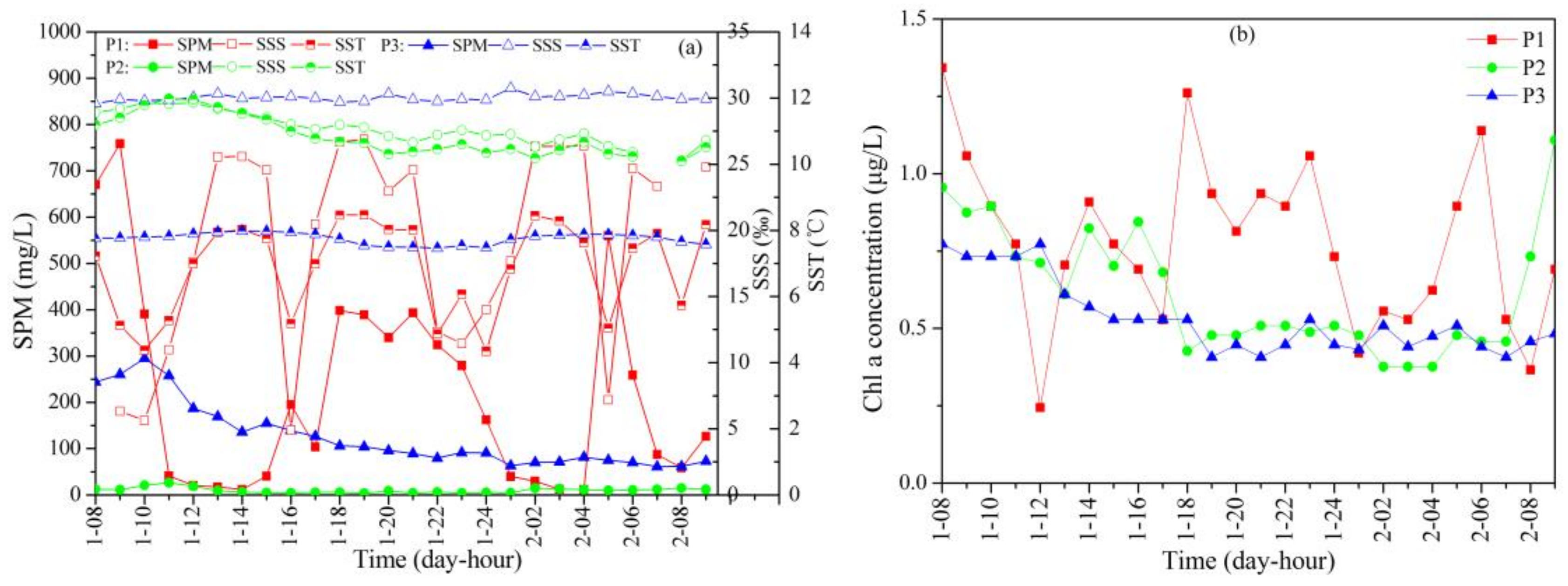
Figure 3.
Time series of wind speed coming from NCEP around the Yellow River Estuary in: (a) November 2011; and (b) December 2011. (c) Time series of in-situ wind speed during the observation period at Stations P1 (open squares, N = 27), P2 (open circles, N = 27) and P3 (solid triangles, N = 27). The red lines indicate the dates when measurements were taken. Wind speed at Station P3 was higher than that at Stations P1 and P2, with the maximum wind speed up to 10.4 m/s. Strong winds occurred on 7 and 10 December before observation, with the highest wind speeds of approximately 14.2 m/s and 12.0 m/s, respectively.

Figure 4.
Spectral curve of CDOM absorption (a); and the CDOM absorption coefficient at 440 nm (b) at Stations P1 (red lines, N = 23), P2 (green lines, N = 25) and P3 (blue lines N = 24). The results show significant differences of diurnal variation of CDOM absorption at different stations.
Figure 4.
Spectral curve of CDOM absorption (a); and the CDOM absorption coefficient at 440 nm (b) at Stations P1 (red lines, N = 23), P2 (green lines, N = 25) and P3 (blue lines N = 24). The results show significant differences of diurnal variation of CDOM absorption at different stations.
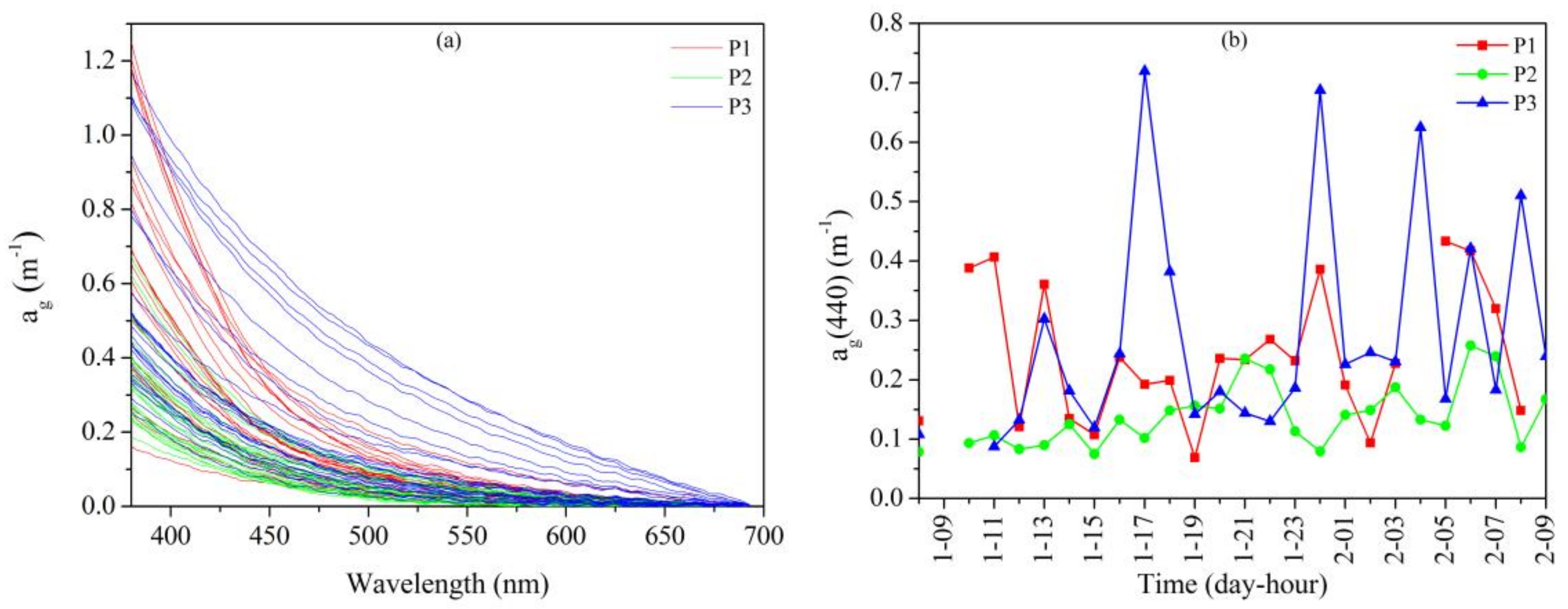
Figure 5.
Relationships of: ag(440) vs. SSS (a); and ag(440) vs. SST (b), at Stations P1 (red squares, N = 21), P2 (green circles, N = 24) and P3 (blue triangles, N = 24). The solid line represents the linear regression with SSS and SST for ag(440). A general trend of decreasing CDOM with increasing SSS and SST was observed for Station P1 and Station P2, but not observed for Station P3.
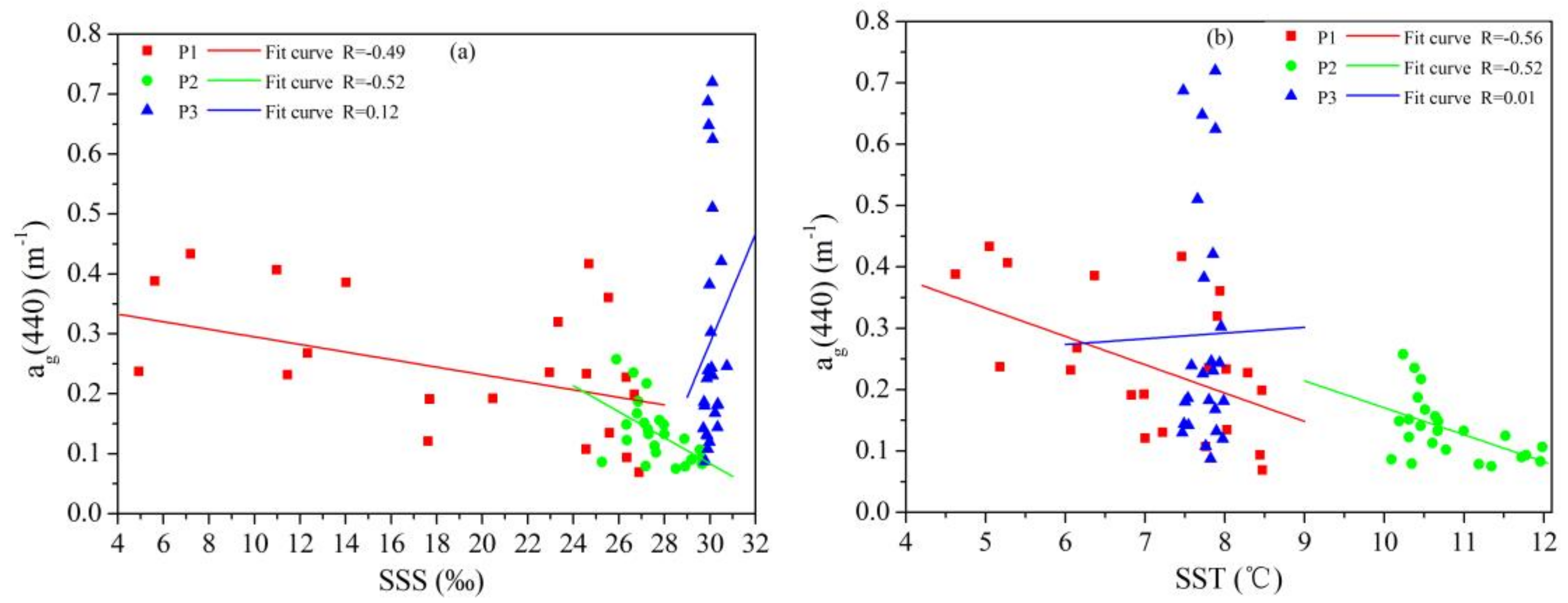
Figure 6.
Power law relationship between ag(440) and Sg (a), and inverse linear relationship between the logarithm of ag(440) and Sg (b), at Stations P1 (red squares, N = 23), P2 (green circles, N = 25), and P3 (blue triangles, N = 24). The solid lines represent the fitted lines using the equations shown in the figure. The coefficients of determination R2 are shown in the figure. There is a strong negative relationship between ag(440) and Sg at Station P3, and a weak negative relationship at Station P2, but no observed relationship at Station P1.

Figure 7.
Spectral curves of: total particle absorption (a); and non-algal particle absorption (b), at Stations P1 (red lines, N = 16), P2 (green lines, N = 22) and P3 (blue lines, N = 18). Note that the magnitude of the spectral absorption coefficient for total particles was nearly similar to that for non-algal particles.
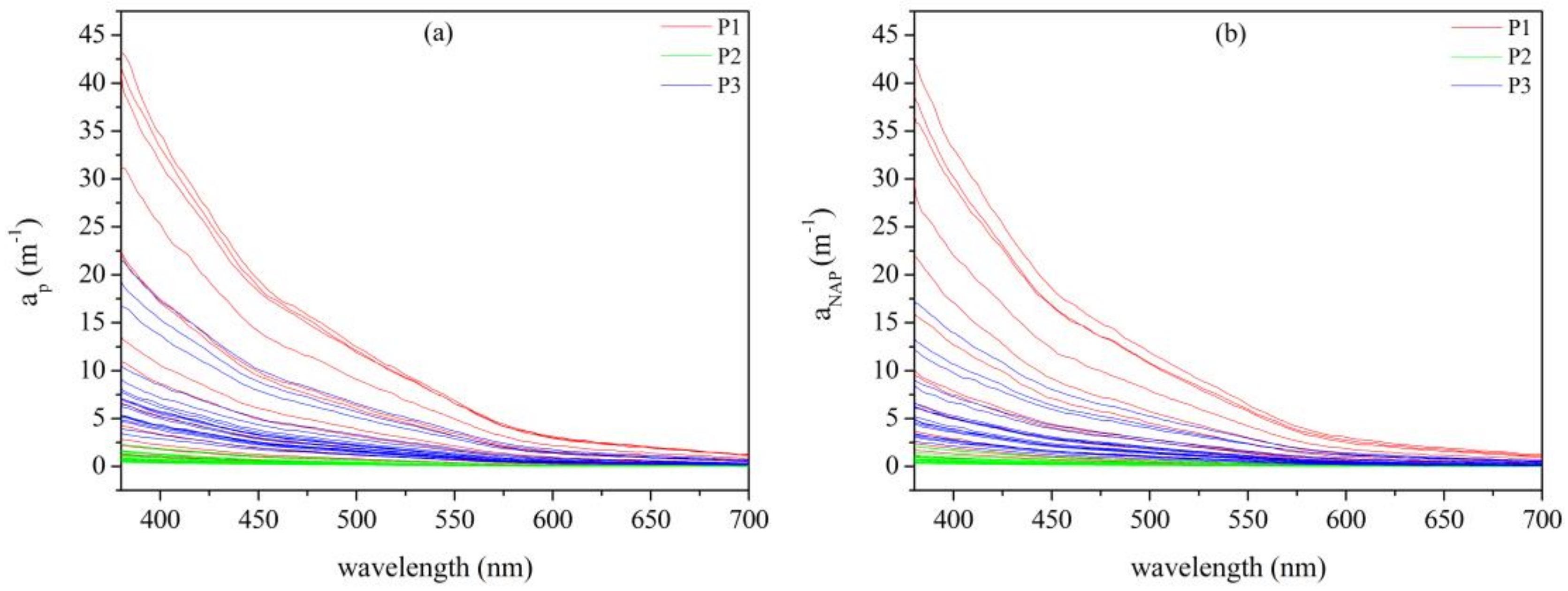
Figure 8.
Variations of the non-algal to total particle absorption ratio (aNAP/ap) at different wavelengths as a function of the SPM concentration at Stations P1 (squares, N = 16), P2 (circles, N = 22) and P3 (triangles, N=18). Different colors represent different wavelengths. The contributions of aNAP(λ) to ap(λ) were more than 56.4% and 60.7% at all main wavelengths for Stations P1 and P3.

Figure 9.
Hourly non-algal particles absorption coefficients at 440 nm at Stations P1 (red squares, N = 16), P2 (green circles, N = 22) and P3 (blue triangles, N=18). The diurnal variation of aNAP(440) showed significant difference for Stations P1, P2 and P3.
Figure 9.
Hourly non-algal particles absorption coefficients at 440 nm at Stations P1 (red squares, N = 16), P2 (green circles, N = 22) and P3 (blue triangles, N=18). The diurnal variation of aNAP(440) showed significant difference for Stations P1, P2 and P3.

Figure 10.
Relationship between aNAP(440) and SPM at Stations P1 (red squares, N=16), P2 (green circles, N = 22) and P3 (blue triangles, N = 18). The solid line represents the linear regression with SPM for aNAP(440), and the coefficients of determination R2 are shown in the figure. Note that there was a positive linear relationship between aNAP(440) and SPM for Stations P1, P2 and P3 with a correlation coefficient R2 greater than 0.75.
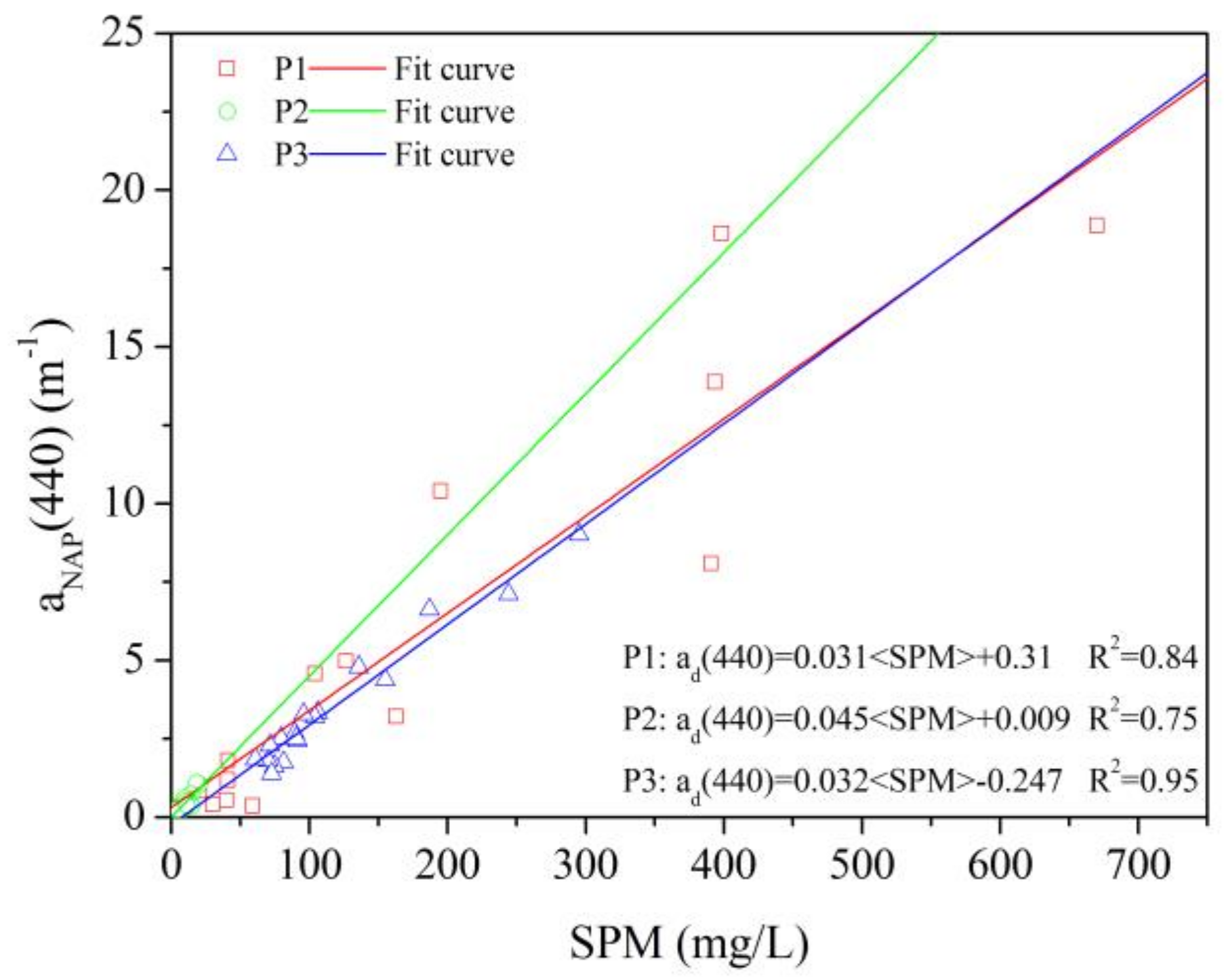
Figure 11.
Ternary plots presenting the relative contribution of absorption by non-algal particles, phytoplankton pigments, and CDOM to total absorption by non-water constituents at different wavelengths at: (a) Station P1 (N = 15); (b) Station P2 (N = 23); and (c) Station P3 (N = 16). Different colors represent different wavelengths.

Figure 12.
Remote sensing reflectance (Rrs(λ)) at different GOCI bands at Stations P1, P2 and P3 derived from GOCI images on 22 September (N = 8), 16 October (N = 8), 25 October (N = 7) and 13 November 2011 (N = 6). Different colors represent different stations. Note that the magnitude of diurnal variation of Rrs at Station P1 was larger than they were at Station P2 and P3 for all four days.

Figure 13.
SD (standard deviation) maps of GOCI retrieved Rrs(680) in the Yellow River Estuary and its adjacent areas on 22 September, 16 October, 25 October and 13 November 2011. Note that the major regions of Rrs(680) diurnal variation were generally located in near-coastal waters and in the estuary of the Yellow River.
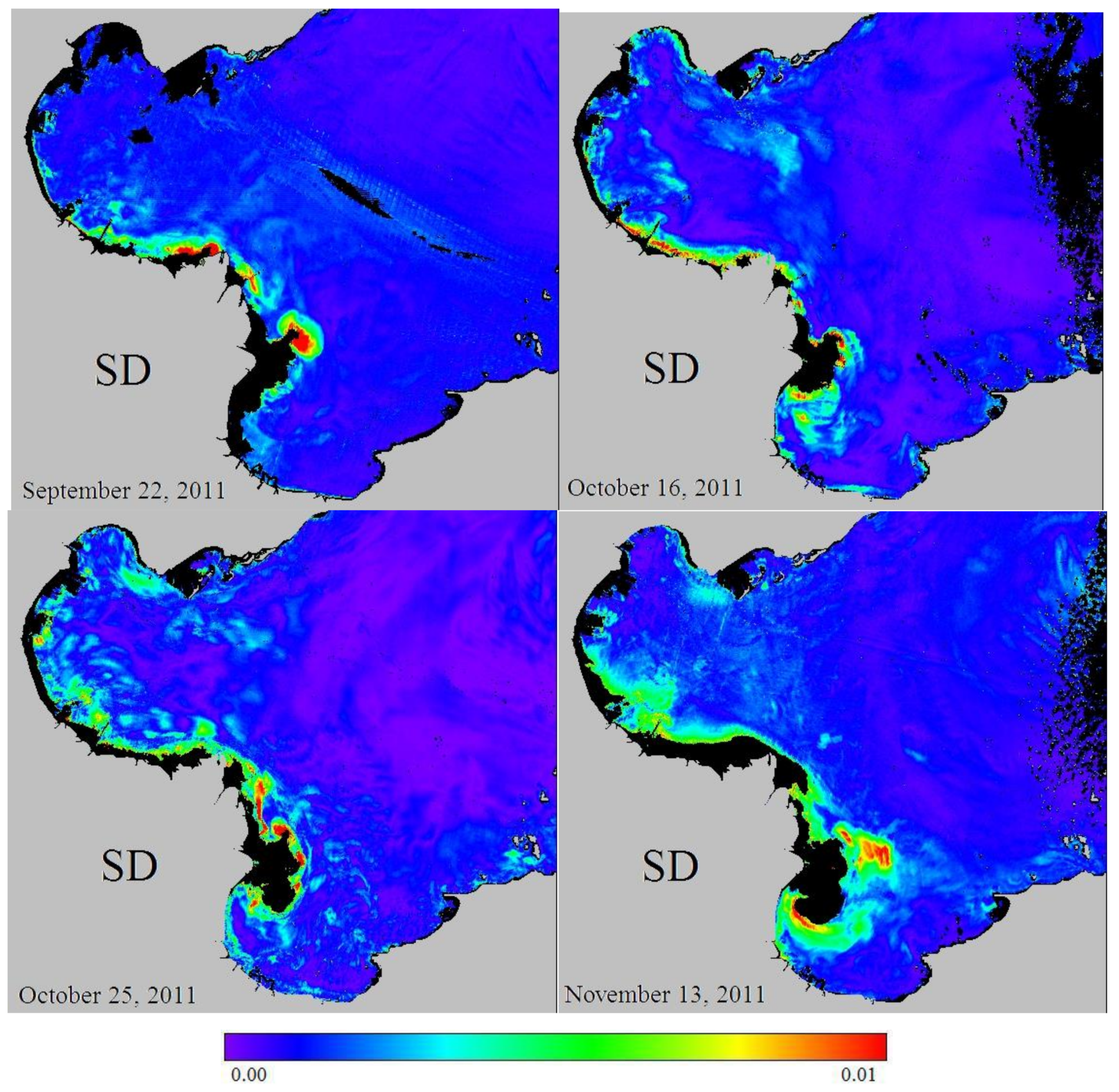
Figure 14.
Time series of the Yellow River flow discharge and sediment concentration at Lijin hydrological gauging station in 2011. The flow discharge distribution had two high peaks from late June to early July and from late September to early October, respectively, which was mainly due to reservoir’s flood relief in the Yellow River upstream.


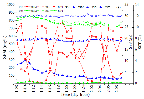
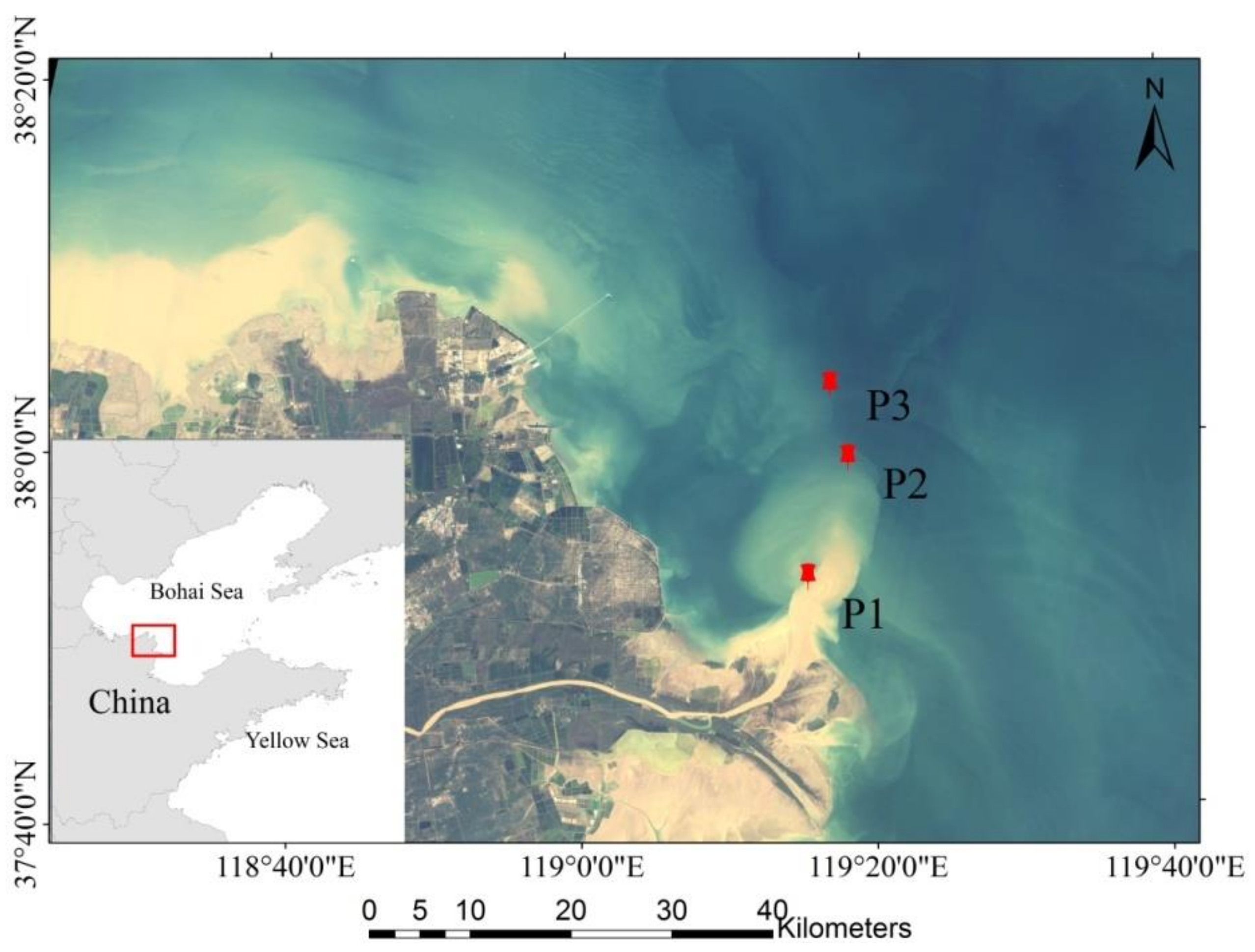
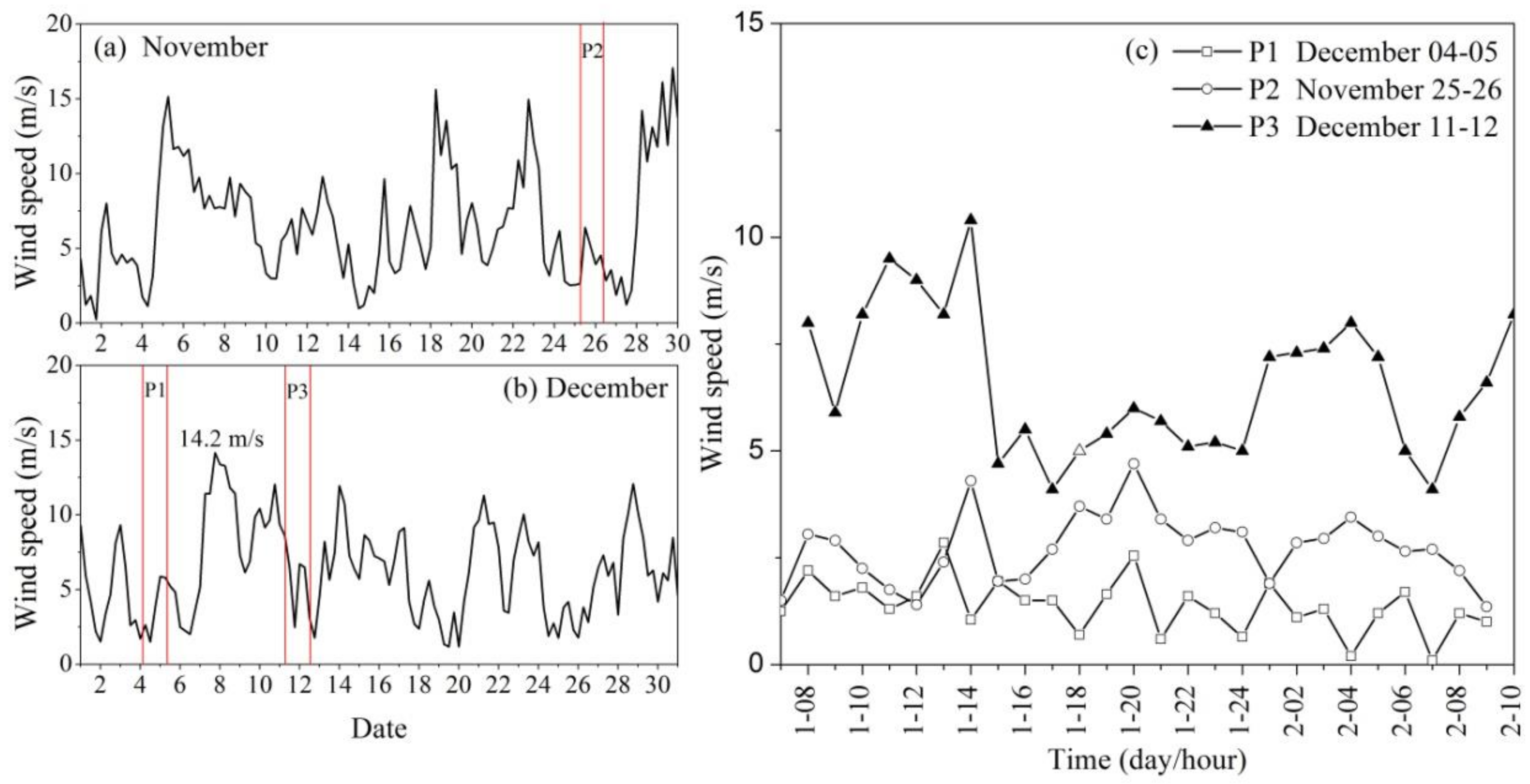
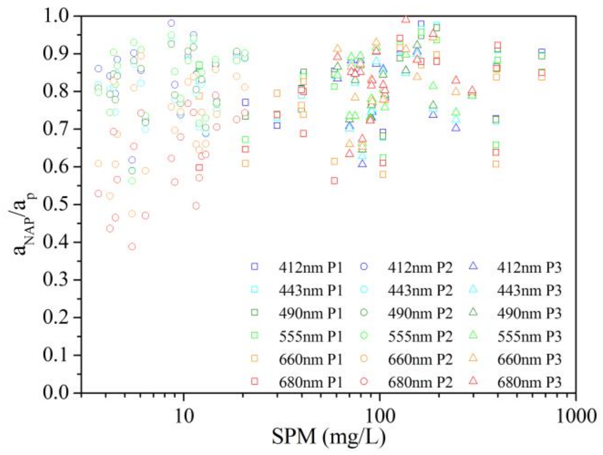
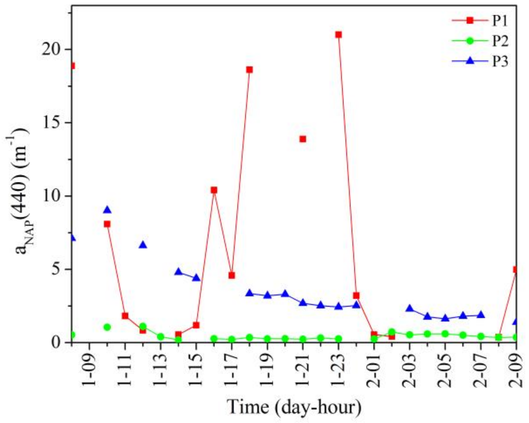
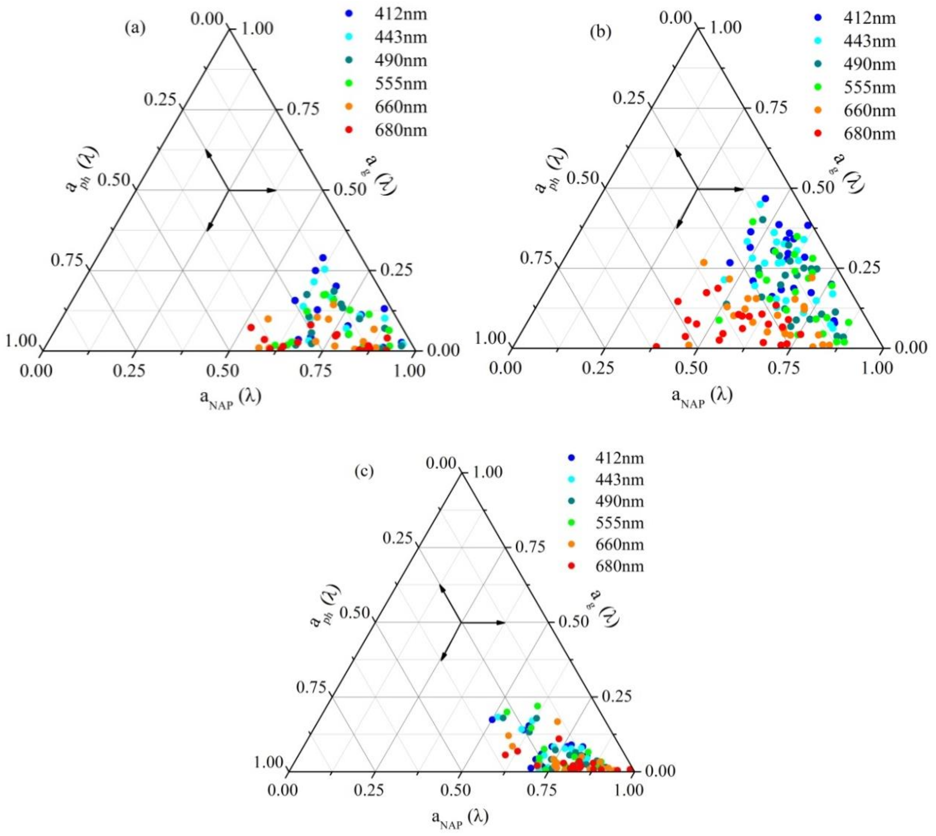
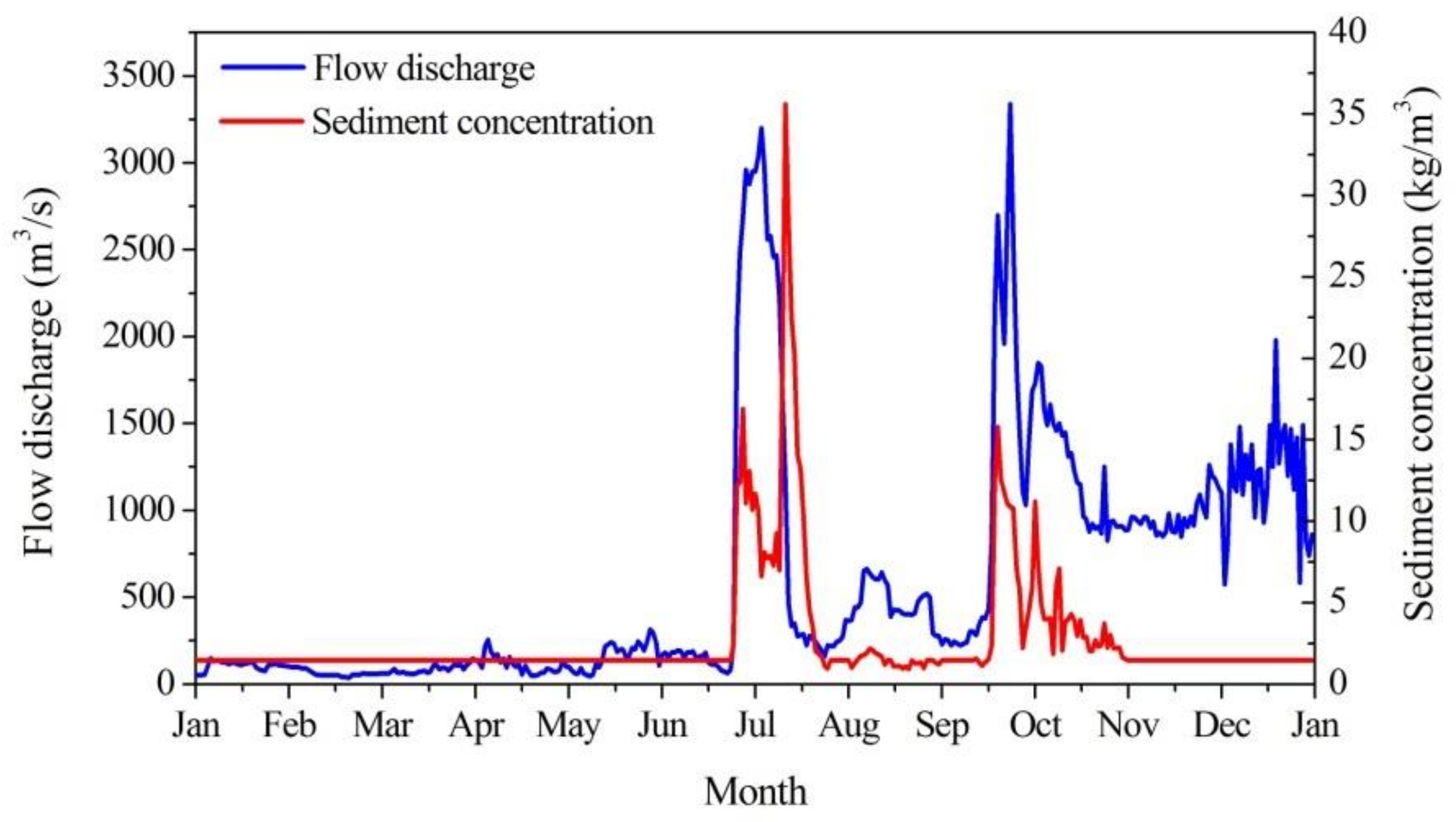
Table 1.
Statistics of SPM and Chl-a concentration measured at Stations P1, P2 and P3. “Max.”, “Min.”, and “SD“ stand for maximum, minimum and standard deviation, respectively, and “N” is the number of samples.
Table 1.
Statistics of SPM and Chl-a concentration measured at Stations P1, P2 and P3. “Max.”, “Min.”, and “SD“ stand for maximum, minimum and standard deviation, respectively, and “N” is the number of samples.
| Stations | SPM (mg/L) | Chl-a (μg/L) | ||||||||
|---|---|---|---|---|---|---|---|---|---|---|
| Max. | Min. | Mean | SD | N | Max. | Min. | Mean | SD | N | |
| P1 | 758.69 | 11.92 | 220.00 | 216.44 | 26 | 1.34 | 0.24 | 0.78 | 0.27 | 26 |
| P2 | 26.45 | 3.67 | 9.95 | 5.68 | 26 | 1.11 | 0.38 | 0.62 | 0.20 | 26 |
| P3 | 295.22 | 60.87 | 125.09 | 69.67 | 26 | 0.77 | 0.41 | 0.53 | 0.12 | 26 |
Table 2.
CDOM absorption coefficients at 440 nm in the Yellow River Estuary at different stations. “Max.”, “Min.”, and “SD” stand for maximum, minimum, and standard deviation, respectively, and “N” is the number of samples.
Table 2.
CDOM absorption coefficients at 440 nm in the Yellow River Estuary at different stations. “Max.”, “Min.”, and “SD” stand for maximum, minimum, and standard deviation, respectively, and “N” is the number of samples.
| ag(440) | Max. (m−1) | Min. (m−1) | Mean (m−1) | SD (m−1) | N |
|---|---|---|---|---|---|
| P1 | 0.43 | 0.07 | 0.24 | 0.11 | 23 |
| P2 | 0.26 | 0.08 | 0.14 | 0.05 | 25 |
| P3 | 0.72 | 0.09 | 0.29 | 0.20 | 24 |
Table 3.
CDOM absorption spectral slopes (Sg) at Stations P1, P2 and P3. “Max.”, “Min.”, and “SD” stand for maximum, minimum, and standard deviation, respectively, and “N” is the number of samples.
Table 3.
CDOM absorption spectral slopes (Sg) at Stations P1, P2 and P3. “Max.”, “Min.”, and “SD” stand for maximum, minimum, and standard deviation, respectively, and “N” is the number of samples.
| Sg | Max. (nm−1) | Min. (nm−1) | Mean (nm−1) | SD (nm−1) | N |
|---|---|---|---|---|---|
| P1 | 0.021 | 0.012 | 0.017 | 0.002 | 23 |
| P2 | 0.020 | 0.012 | 0.016 | 0.002 | 25 |
| P3 | 0.018 | 0.008 | 0.013 | 0.003 | 24 |
Table 4.
Statistics of non-algal particles absorption coefficients at 440 nm at different stations. “Max.”, “Min.”, and “SD” stand for maximum, minimum, and standard deviation, respectively, and “N” is the number of samples.
Table 4.
Statistics of non-algal particles absorption coefficients at 440 nm at different stations. “Max.”, “Min.”, and “SD” stand for maximum, minimum, and standard deviation, respectively, and “N” is the number of samples.
| aNAP(440) | Max. (m−1) | Min. (m−1) | Mean (m−1) | SD (m−1) | N |
|---|---|---|---|---|---|
| P1 | 21.01 | 0.37 | 6.84 | 7.42 | 16 |
| P2 | 1.10 | 0.18 | 0.44 | 0.25 | 22 |
| P3 | 9.02 | 1.40 | 3.48 | 2.08 | 18 |
Table 5.
Non-algal particle absorption spectral slopes SNAP at Stations P1, P2 and P3. “Max.”, “Min.”, and “SD” stand for maximum, minimum, and standard deviation, respectively, and “N” is the number of samples.
Table 5.
Non-algal particle absorption spectral slopes SNAP at Stations P1, P2 and P3. “Max.”, “Min.”, and “SD” stand for maximum, minimum, and standard deviation, respectively, and “N” is the number of samples.
| Derived SNAP | Max | Min | Mean | SD | N |
|---|---|---|---|---|---|
| P1 | 0.0120 | 0.0104 | 0.0113 | 0.00042 | 16 |
| P2 | 0.0115 | 0.0100 | 0.0108 | 0.00035 | 22 |
| P3 | 0.0108 | 0.0097 | 0.0103 | 0.00029 | 18 |
Table 6.
Rrs(680) derived from GOCI images on 22 September, 16 October, 25 October and 13 November 2011. “Max.”, “Min.”, and “SD” stand for maximum, minimum, and standard deviation, respectively, and “N” is the number of samples.
Table 6.
Rrs(680) derived from GOCI images on 22 September, 16 October, 25 October and 13 November 2011. “Max.”, “Min.”, and “SD” stand for maximum, minimum, and standard deviation, respectively, and “N” is the number of samples.
| Rrs(680) (sr−1) | 22 September 2011 | 16 October 2011 | ||||||||
|---|---|---|---|---|---|---|---|---|---|---|
| Max. | Min. | Mean | SD | N | Max. | Min. | Mean | SD | N | |
| P1 | 0.0366 | 0.0140 | 0.0236 | 0.0092 | 8 | 0.0404 | 0.0137 | 0.02340 | 0.0091 | 8 |
| P2 | 0.0105 | 0.0053 | 0.0079 | 0.0019 | 8 | 0.0060 | 0.0041 | 0.0054 | 0.0007 | 8 |
| P3 | 0.0093 | 0.0035 | 0.0052 | 0.0017 | 8 | 0.0048 | 0.0031 | 0.0039 | 0.0006 | 8 |
| 25 October 2011 | 13 November 2011 | |||||||||
| P1 | 0.0421 | 0.0203 | 0.0280 | 0.0080 | 7 | 0.0383 | 0.0251 | 0.0341 | 0.0054 | 6 |
| P2 | 0.0250 | 0.0143 | 0.0201 | 0.0042 | 7 | 0.0207 | 0.0152 | 0.0189 | 0.0021 | 6 |
| P3 | 0.0227 | 0.0175 | 0.0201 | 0.0021 | 7 | 0.0160 | 0.0124 | 0.0146 | 0.0015 | 6 |
© 2018 by the authors. Licensee MDPI, Basel, Switzerland. This article is an open access article distributed under the terms and conditions of the Creative Commons Attribution (CC BY) license (http://creativecommons.org/licenses/by/4.0/).
Share and Cite
MDPI and ACS Style
Hao, Y.; Cui, T.; Singh, V.P.; Zhang, J.; Yu, R.; Zhao, W. Diurnal Variation of Light Absorption in the Yellow River Estuary. Remote Sens. 2018, 10, 542. https://doi.org/10.3390/rs10040542
AMA Style
Hao Y, Cui T, Singh VP, Zhang J, Yu R, Zhao W. Diurnal Variation of Light Absorption in the Yellow River Estuary. Remote Sensing. 2018; 10(4):542. https://doi.org/10.3390/rs10040542
Chicago/Turabian StyleHao, Yanling, Tingwei Cui, Vijay P. Singh, Jie Zhang, Ruihong Yu, and Wenjing Zhao. 2018. "Diurnal Variation of Light Absorption in the Yellow River Estuary" Remote Sensing 10, no. 4: 542. https://doi.org/10.3390/rs10040542
Note that from the first issue of 2016, this journal uses article numbers instead of page numbers. See further details here.