Pole-Like Road Furniture Detection and Decomposition in Mobile Laser Scanning Data Based on Spatial Relations


Faculty of Geo-Information Science and Earth Observation, University of Twente, PO BOX 217, 7514 AE Enschede, The Netherlands
*
Author to whom correspondence should be addressed.
Remote Sens. 2018, 10(4), 531; https://doi.org/10.3390/rs10040531
Submission received: 16 February 2018
/
Revised: 20 March 2018
/
Accepted: 28 March 2018
/
Published: 30 March 2018
(This article belongs to the Special Issue Mobile Laser Scanning)
Abstract
:Road furniture plays an important role in road safety. To enhance road safety, policies that encourage the road furniture inventory are prevalent in many countries. Such an inventory can be remarkably facilitated by the automatic recognition of road furniture. Current studies typically detect and classify road furniture as one single above-ground component only, which is inadequate for road furniture with multiple functions such as a streetlight with a traffic sign attached. Due to the recent developments in mobile laser scanners, more accurate data is available that allows for the segmentation of road furniture at a detailed level. In this paper, we propose an automatic framework to decompose road furniture into different components based on their spatial relations in a three-step procedure: first, pole-like road furniture are initially detected by removing ground points and an initial classification. Then, the road furniture is decomposed into poles and attachments. The result of the decomposition is taken as a feedback to remove spurious pole-like road furniture as a third step. If there are no poles extracted in the decomposition stage, these incorrectly detected pole-like road furniture—such as the pillars of buildings—will be removed from the detection list. We further propose a method to evaluate the results of the decomposition. Compared with our previous work, the performance of decomposition has been much improved. In our test sites, the correctness of detection is higher than 90% and the completeness is approximately 95%, showing that our procedure is competitive to state of the art methods in the field of pole-like road furniture detection. Compared to our previous work, the optimized decomposition improves the correctness by 7.3% and 18.4% in the respective test areas. In conclusion, we demonstrate that our method decomposes pole-like road furniture into poles and attachments with respect to their spatial relations, which is crucial for road furniture interpretation.

1. Introduction
Road safety has been one of the major focuses in public safety concerns for many years. In the 2015 global status report on road safety, the total number of worldwide road traffic deaths remains unacceptably high at 1.25 million per year [1]. To conduct road safety inspections in Europe, a road infrastructure safety management directive is adopted by the European Union [2]. The EU will eventually have a role in the safety management of the roads belonging to European transportation networks—which is set to encompass 90,000 km of motorway and high-quality roads by 2020—through safety audits at the design stage and regular safety inspections of the network [3]. Similar policies also have been made in the U.S. In 2014, the U.S. Department of Transportation developed a system named Model Inventory of Roadway Elements (MIRE) to inventory road furniture and improve roadway safety [4]. Road safety can be enhanced by the inventory of road furniture which is strongly related to road furniture detection [5].
Another rising general interest is autonomous driving, which facilitates driving safety and makes life more convenient. In addition, it enables people such as the aged and disabled who cannot drive to use a vehicle [6]. Although autonomous driving systems do not fully rely on 3D precise maps, it is still crucial for the improvement of the safety and stability of automatic driving systems. Road furniture detection plays an important role in both road furniture inventory and 3D highly precise mapping, which consists of road detection, curbstone detection, pole-like road furniture interpretation, and so forth.
Currently, the road furniture inventory mainly relies on visual inspection or semi-manual interpretation, which is time-consuming and tedious. To facilitate this procedure, methods for automatic road furniture detection relying on high-quality data are needed. Tools for capturing three-dimensional road scene data are Mobile Mapping Systems (MMS) which have been developed rapidly in recent years. They are often mounted on a vehicle and mainly composed of four parts: Light Detection and Ranging (LiDAR) sensors that collect 3D point clouds, cameras that capture 2D imagery data, an accurate Global Positioning System (GPS) that records the position of the previous two sensors, and an Inertial Measure Unit (IMU) that measures the pose of the sensors. Compared with optical images acquirement, Mobile Laser Scanning (MLS) data collection is not restricted by the illumination conditions such as good weather and daytime. Moreover, MLS data can be obtained rapidly and accurately. Significant progress has been made on research related to road furniture inventory in the laser scanning data field, which includes road detection and modelling [7,8,9], curbstones mapping [10], railway modelling [11,12], pole-like road furniture interpretation [13,14,15,16,17,18,19,20,21], tree inventory [22], and building detection [23,24,25,26]. In the urban scene, MLS data analysis has become popular and essential for urban road environment analysis.
Individual road furniture can be interpreted as a single object or as multiple connected parts. For instance, a streetlight with an attached traffic sign can be recognized as a streetlight at the object level. It can also be interpreted as multiple connected parts: a pole connected to a traffic sign and a streetlight. Numerous studies have been carried out on road furniture interpretation on the level of single objects, while only a little attention has been paid to the more detailed segmentation of road furniture based on spatial relations between object parts. Such a detailed segmentation, however, is necessary since it provides more detailed partition information for the interpretation of road furniture. The objective of this paper is to propose an automatic framework for road furniture decomposition.
The rest of the paper is organized as follows. Section 2 provides a review of related work on road furniture interpretation and state of art of point cloud semantics segmentation techniques. In Section 3, our method is described in three main stages: the initial road furniture detection, decomposition, and final road furniture detection. We introduce the test sites, analyze the experimental results, and give a comparison to other work in Section 4. The conclusions that are drawn and possible future work can be found in Section 5.
2. Related Work
The reliability of MLS systems has improved remarkably in recent years. It is reported that the accuracy of the advanced mobile laser scanning system is as high as 5 mm under a 30 m range [27]. Its ability to acquire road objects’ 3D structural information, which 2D optical cameras cannot directly capture, is highlighted. An important factor of MLS data is the varying point density which impacts the performance of 3D point cloud interpretation algorithms. This is because it is difficult to find a reasonable neighboring size for feature extraction under these conditions. There are two elements that affect the point density of MLS data. The first one is the distance between scanners and recorded objects, which causes the change of the point density along the scanline direction. The latter one is the vehicle speed, which adds to the variation of the point density between the different scan lines. Accounting for these properties, numerous studies on MLS data interpretation have been performed. Work on 3D objects interpretation is summarized in two categories: unsupervised methods and supervised methods.
Much research in recent years has focused on road furniture interpretation in the point cloud by using unsupervised methods [13,14,16,17,28,29].
Pu et al. [14] proposed a percentile-based method to recognize pole-like structures from mobile laser scanning data for road inventory studies. Firstly, they used road parts to partition the unorganized MLS data. Then they divided the point clouds into three parts: ground points, points connected to the ground, and off-ground points. Finally, they used knowledge-based methods to recognize the above-ground segments. The method was able to detect 61–87% of poles in the point clouds. Among all the subclasses, the detection rate of trees was the lowest (29.5–63.5%). However, for this method, there are problems with the detection of jointly connected pole-like objects such as trees connected with pole-like objects. Li and Oude Elberink [16] optimized the method of Reference [14] by adding reflectivity information. Because of the use of reflectance information and pulse count information, the rate of street sign detection and tree detection is largely improved. However, connected pieces of road furniture cannot be detected and recognized in these two methods.
Lehtomäki et al. [13] represents an early attempt which detects vertical-pole objects by using scan line segmentation and cylinder fitting. At first, they extracted potential sweeps from the data, removing long segments and keeping short segments. Then the segments are grouped based on their profile information and horizontal plane position before these clusters that belong to one pole are merged by distance and orientation check. Finally, these clusters are classified into poles and non-poles according to their properties, such as height, shape, and orientation. The detection rate of the poles is 77.7% and the correctness is 81.0%. It is hard for this method to detect some complex pole-like objects that contain many points in the outer cylinder such as slanted pole-like road furniture or traffic signs that consist of many signboards. With a similar cylinder model mask, Cabo et al. [17] proposed a voxel-based algorithm to detect pole-like road furniture objects from MLS data. In order to make the point clouds more uniform, they first voxelized the point clouds into grids. Then they analyzed the three-dimensional information using two concentric cylinders. Finally, pole-like objects were classified from point clouds. Although this method has acquired pretty good results, there are still some limitations such as the detection of poles that are too close to bushes or guardrails. Nurunnabi et al. [28] utilized a robust diagnostic principal component analysis (RDPCA) in combination with region growing to segment road furniture into different parts. However, saliency features used in this method strongly rely on a dense point cloud.
Several scholars have put effort into road furniture recognition by introducing supervised approaches [18,30,31,32,33,34,35,36].
Golovinsky et al. [30] utilized a normalized cut method to localize objects of interest. Different machine learning techniques in combination with shape features were used to classify these above-ground objects into sixteen categories. In the work of Munoz et al. [31], a functional gradient approach was proposed to label mobile mapping data by using Max-Margin Markov Networks (M3Ns). This method was tested for both 3D point cloud classification and geometric surface estimation in 2D images. However, this method still found it hard to separate and classify conjunctions which contain multiple objects.
Different from these methods mentioned above, Huang and You [18] proposed a method in combination with a Supported Vector Machine (SVM) to classify road furniture into four categories. In order to localize pole-like objects, they implemented point cloud slicing, clustering, pole seed generation, and bucket augmentation. In the following stage, ground points are removed and the pole-like objects were extracted. In the end, six features are trained by the SVM to classify road furniture into four types. The detection rate of pole-like road furniture was 75%.
Soilán et al. [34] used mobile laser scanning data in combination with images to recognize traffic signs. At the first stage, the ground points were removed by using height and intensity constraints. Traffic signs were extracted with a reflectance threshold estimated by a Gaussian Mixture Model (GMM). Then, geometric parameters of the extracted traffic signs were generated. Based on these geometric inventories, these extracted components were projected onto the corresponding camera systems, after which traffic signs can be found on the corresponding 2D images. In the end, Histogram of Oriented Gradients (HOG) features trained by the SVM are adapted to recognize traffic signs. More than 85% of pole-like traffic signs were detected. However, the detection of traffic signs in this methpd strongly relies on the reflectance information.
Hackel et al. [35] described an efficient and effective method for point-wise semantic classification, which can deal with point clouds captured by LiDAR or derived from photogrammetric reconstruction with high-density variations. Instead of computing optimal neighborhoods for each point, they down-sample the entire point cloud to generate a multi-scale pyramid with decreasing point density and compute features for every voxel at every scale level. Then these features are trained and discriminant ones are selected. Finally, Random Forest (RF) is used for semantically labeling. As a drawback, RF cannot make use of contextual information. The precision of pole-like road furniture recognition is less than 35%.
The Bag of Words (BoW) and Deep Boltzmann Machine (DBM) methods are applied by Yu et al. [36] to detect and recognize traffic signs in mobile laser scanning (MLS) data. Here, the authors first constructed a visual word vocabulary by using features encoded by a DBM model to detect traffic signs. Similar to Li et al. [29], they separated the poles and traffic signs which are projected to 2D images afterward. Lastly, these cropped traffic sign images were recognized by a pre-trained DBM model. More than 90% of pole-like road furniture was detected in the high-quality MLS data. A 3D convolutional neural network was proposed by Huang and You [33] to interpret urban scenes into seven categories. They first used small grids to densely voxelize the original point cloud. Then feature maps in combination with a convolutional neural network are trained to label the point clouds. 87% of pole-like road furniture were identified.
Compared to unsupervised methods, supervised methods are more flexible in multi-class identification problems. Normally, supervised methods need a lot of training data. For one-class detection problems, unsupervised methods are more practical, especially when there is a limited amount of training data. How to leverage these two methods or combine them still needs to be explored. In this paper, we use a knowledge-driven method—in which generic rules are defined—to detect and decompose road furniture.
All in all, significant progress has been achieved on 3D object classification and 3D scene labeling. Nevertheless, no attention has been paid to the road furniture partitioning based on shape constraints of different components, which is the innovation presented by this paper.
3. Methodology
In this section, the three main stages of our framework are presented: the initial road furniture detection (Section 3.1), decomposition (Section 3.2), and the final road furniture detection (Section 3.3). Firstly, road furniture were initially extracted from unorganized mobile laser scanning points. In the following stage, these detected road furniture objects were decomposed into poles and attachments based on their spatial relations. Road furniture detection is then refined by the feedback of road furniture decomposition (Section 3.3). In addition, we introduced an approach to evaluate the result of the decomposition which is explained in Section 3.4. The workflow of our framework is illustrated in Figure 1.
3.1. Initial Detection of Road Furniture
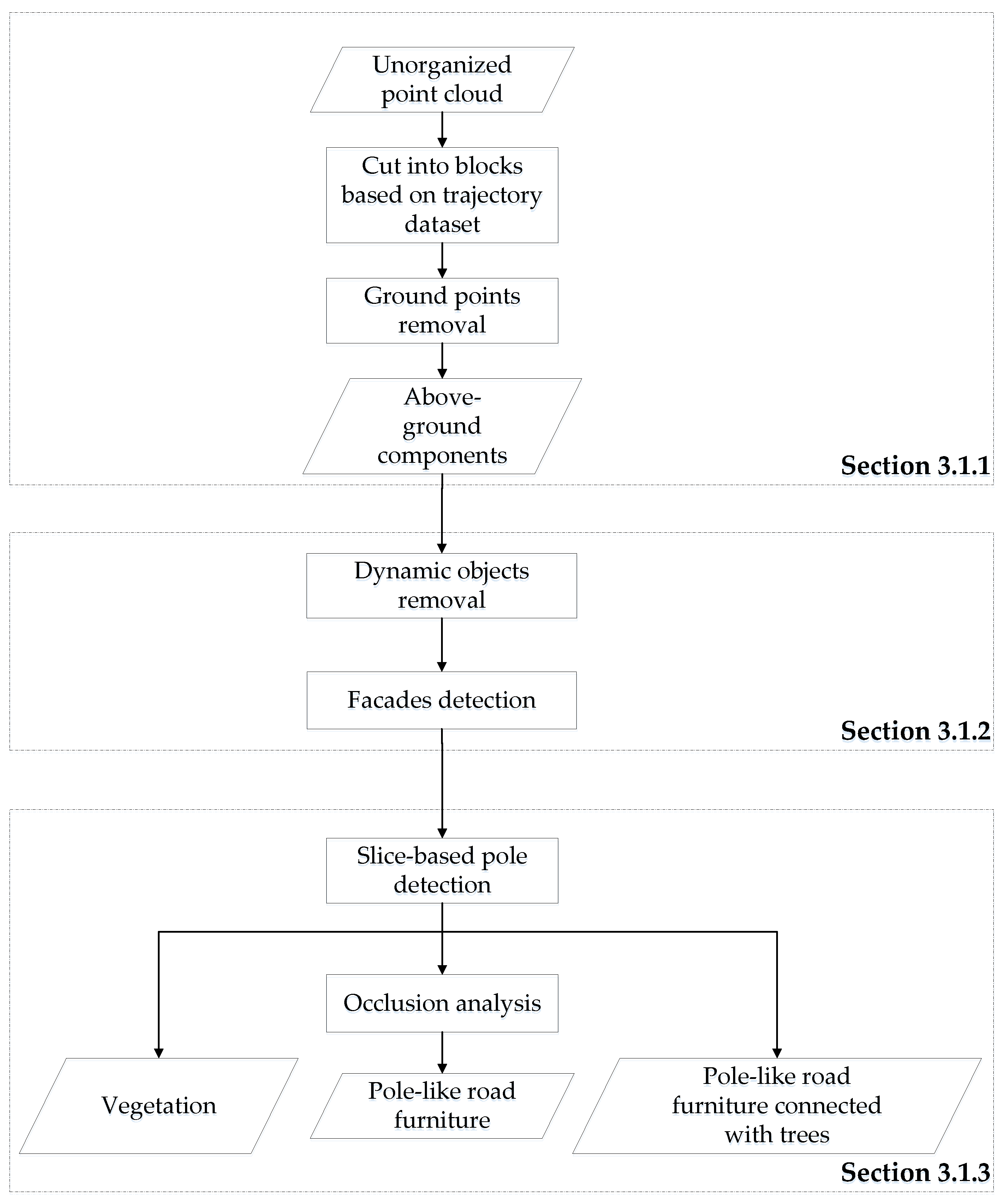
The main objective of this paper is to segment road furniture within a certain distance from laser scanners. It is difficult to segment long distance points that are captured with scanners because of their low point density. Therefore, we defined a distance to remove points that are far away from the road (trajectory line), which also helps to reduce the computation cost. At this stage, we started with pre-processing, which divided the unstructured data into roadblocks, removed the ground points, and obtained the above-ground components. Then, an initial classification was performed to remove dynamic objects and detect building components. In the last step, we proposed a slice-based method to extract pole-like road furniture, trees, and pole-like road furniture connected with trees and excluded objects inside buildings by occlusion analysis. The workflow of the initial pole-like road furniture detection is as shown in Figure 2.
3.1.1. Pre-Processing
The original mobile laser point cloud files are often very large and result in computation and memory problems when processed in one go. To circumvent these difficulties, we split the unorganized point cloud into road parts along the trajectory line as described in Reference [14]. In this paper, the length and width of a road part are specified as 50 m and 40 m, respectively. Since one piece of road furniture could be separated into two parts, the length of the overlapping zone between two neighboring road parts is set to 5 m.
Ground points are the main connection between different above-ground objects. In order to separate different objects, ground points should be removed first. After splitting the point cloud into road parts, the ground points were removed in each road part. As the road surfaces are smooth, the height difference between all nearby points within a certain neighborhood was small. In contrast, for above-ground objects, there was a large height difference between all nearby points within a certain neighborhood. We calculated the height difference as the difference between the maximum height and the minimum height within a point’s neighborhood [37]. In this paper, the neighborhood size was set to be quite large (e.g., 100 nearest neighboring points) because of the high point density of the ground points. When the point cloud is very sparse, it should be set lower. The height difference threshold was set to be 0.15 m. Based on this property, the ground points were removed. Compared to surface growing, this method proved to be more efficient.
After the ground points are removed, the remaining above-ground points were clustered by conducting a connected component analysis. This resulted in the above-ground objects for the initial classification.
3.1.2. Initial Classification
During the collection of MLS data, many moving objects or pedestrians were scanned. These unrelated objects should be removed to mitigate false positive detection of road furniture. As mentioned in the introduction, our objects of interest were road-side objects which were assumed to have traffic functionalities. However, large building façades also frequently occur in road environments. Consequently, it is necessary to remove them to reduce the computational effort for road furniture detection. On the other hand, buildings façades can provide useful information for pole-like road furniture detection. For instance, some pole-like objects inside buildings can be eliminated by using façade information. In this research, dynamic objects, buildings, and fences that are not related to road furniture were labeled thusly in this period and removed before decomposition.
In the initial classification, we use the method described in Reference [37] to remove dynamic objects. A component was labeled as a dynamic object if more than 90% of the points only had k-neighbors from the same scanner. This can only be used for the data collected by multiple laser scanners. A detailed explanation is given in Reference [37].
A large number of building points in the point cloud would lead to an unnecessarily high computation time. Compared to other road objects, a façade plane is perpendicular to the ground, its area is large, and it is above a certain height. Similar to the method in References [23,24], the orientation, height, and area of the façade were selected as distinctive features to detect the façade components. In this step, surface growing was utilized to extract the planes from the components. Based on an area and angle threshold, the large vertical planes were retained afterward.
3.1.3. Slice-Based Pole-Like Road Furniture Detection
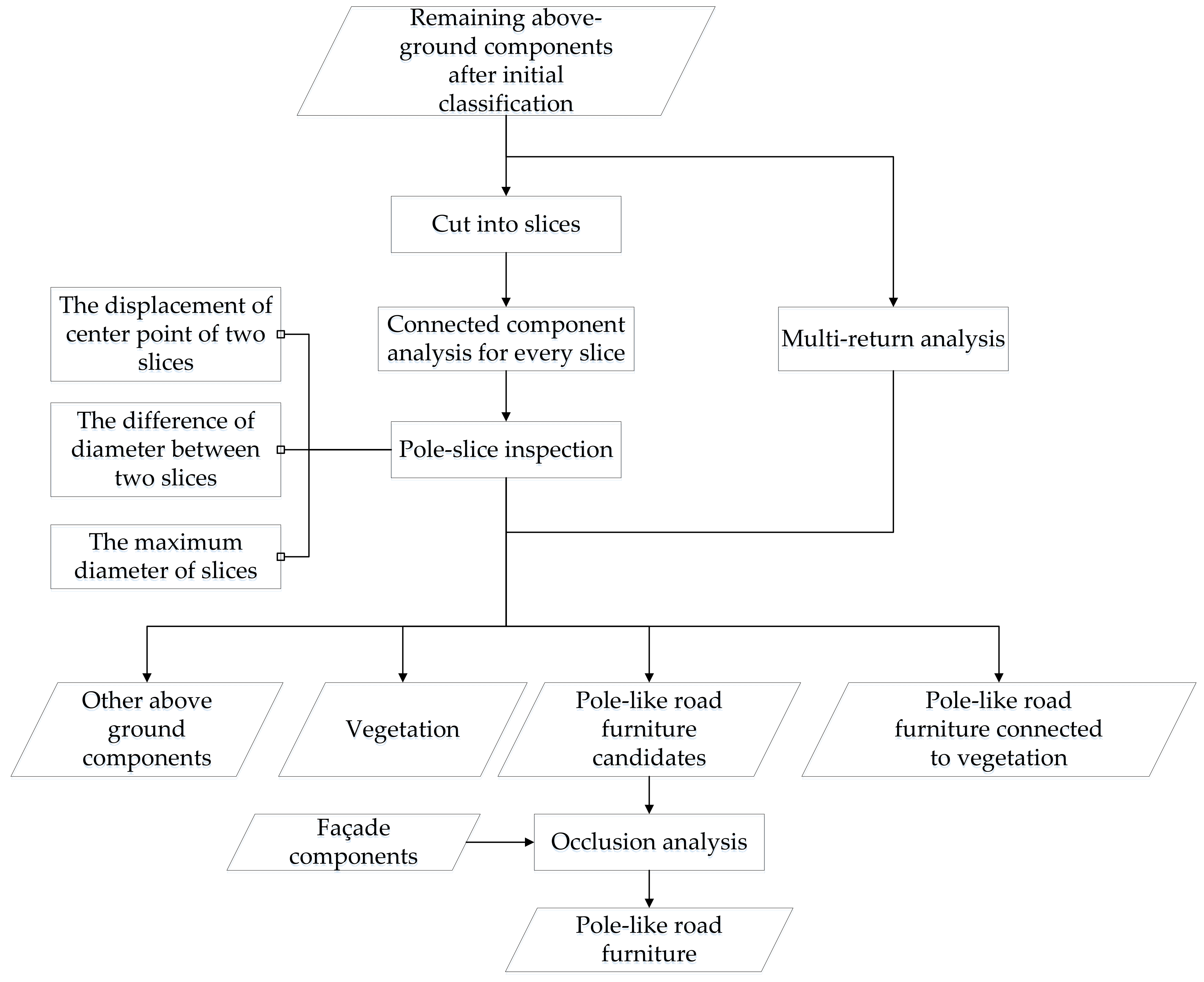
In this step, pole-like road furniture, vegetation, and pole-like road furniture connected to vegetation were extracted. As known, many types of vegetation have small branches and massive leaves. When a laser pulse hits small branches or leaves, this pulse usually splits into multiple pulses before reaching the receiver sensor. In contrast, most points of other objects exclusively have a single pulse count attribute [38]. Consequently, the ratio of points with a multi-pulse count is useful for tree detection. However, there are points which belong to the edges of road furniture with multiple counts as well. If we use the number of returns, the points belong to the edges of above-ground objects are also labeled with multiple returns. Therefore, the value of the return number was utilized instead of the number of returns as a feature to extract trees. In our research, the ratio of points with the first return in above-ground components was also used as a feature to detect trees. In order to extract pole-like road furniture, Pu et al. [14] proposed a framework which allows for the general interpretation of road furniture. Their work represents an early attempt to utilize a percentile-based algorithm to detect pole-like road furniture. However, it has difficulty in detecting road furniture with a large number of attached components. For instance, it has difficulty extracting traffic lights that are connected to many traffic signs and street signs. To overcome these difficulties, a slice-based method was presented to detect pole-like road furniture. Occlusion analysis was used to remove pole-like objects behind façades afterward. The workflow of this method is as shown in Figure 3.
First, every individual above-ground component was cut into horizontal slices (Figure 4). Then a connected component analysis was performed for every slice to produce separated components. The center point of every separated slice component was computed and a 2D connected component analysis was applied to connect the components which were very close to each other in the horizontal plane. Here, three constraints were applied to compute the number of pole-slices for the connected slice components in every individual above-ground component. The first constraint was the displacement of the center points of two neighboring slices (Figure 4). There should be no large displacement between the two neighboring slices. The second one was the difference of the diameter of two neighboring slices. The diameter of a slice was the 2D largest distance between two points in this slice. The difference of diameters between the two neighboring slices should be small (e.g., 0.2 m), assuming that a part of the pole will have no attached objects. The third constraint was the diameter of a slice (Figure 4). The diameter of a slice should be smaller than a pre-determined threshold. Finally, the number of pole slices was checked for every individual above-ground component. If the number of pole-slices was larger than a specified threshold (set to 3) and the ratio was smaller than a threshold (0.05), this component was labeled a pole-like road furniture. If the number of pole slices was larger than a specified threshold and the ratio was larger than the threshold, this component was labeled a pole-like road furniture connected to trees. If both of them were smaller than their corresponding thresholds, this component was labeled trees.
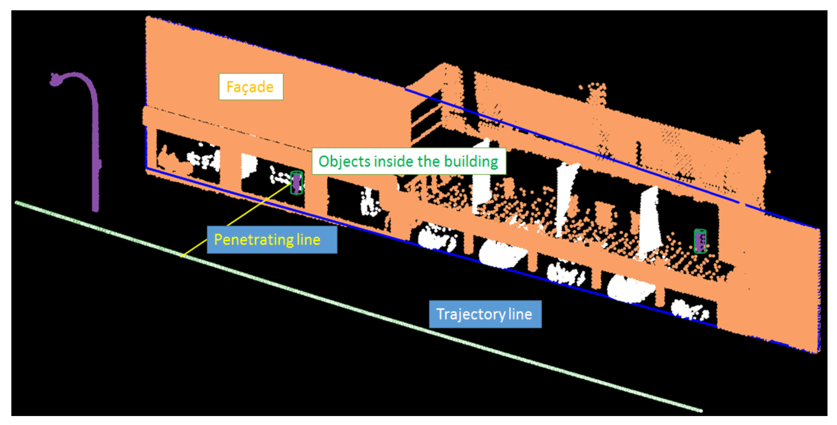
Among the detected pole-like road furniture candidates, there were incorrectly detected objects which were located behind façades. To exclude them, an occlusion analysis is performed. In the step of the initial classification, façade planes were obtained through surface growing. Then these façade planes were computed as constraints to determine if these pole candidates were located outside of the façade planes (Figure 5). If they were positioned outside of the façade, they were labeled as pole-like road furniture, otherwise, they were not.
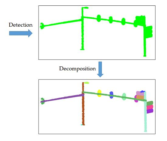
3.2. Road Furniture Decomposition
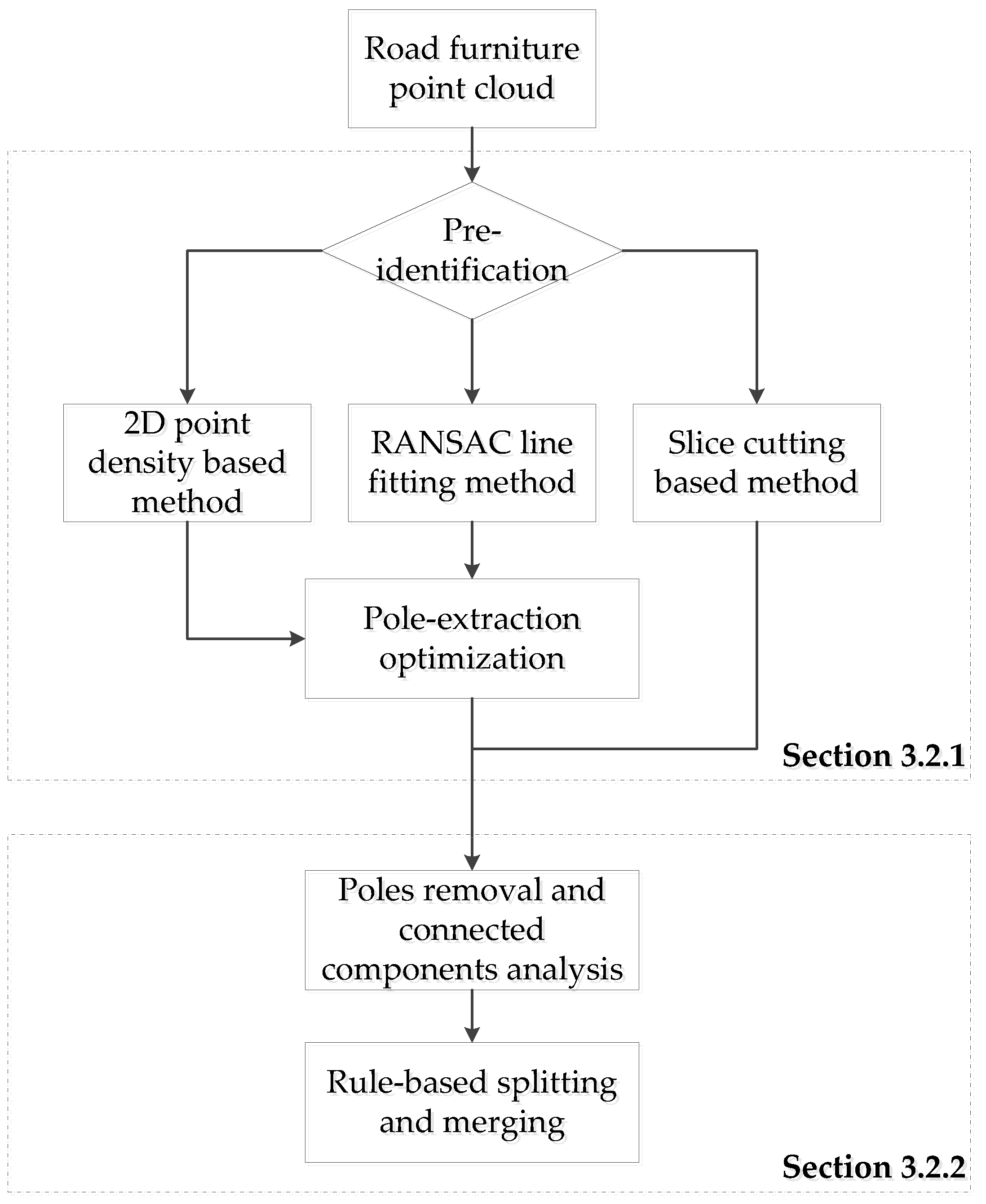
To address the problem that some road furniture had multiple functions, we presented a new method to decompose road furniture into different components based on their spatial relations. We analyzed the relationship between attachments and vertical and horizontal poles. Therefore, it is crucial to know which points belong to which pole. The remaining points have spatial relations to either horizontal or vertical poles. Based on these relations, we presented an optimal segmentation procedure. The overall workflow of this method is as shown in Figure 6. There is a large variety of structures and shapes in pole-like road furniture. It is difficult to extract all the poles using a single method. Therefore, we first identified some key properties of the road furniture, based on which the most suitable pole extraction method was selected (Section 3.2.1). Next, the poles were removed and the attached components were separated into different parts (Section 3.2.2). In the end, the rule-based splitting and merging were carried out to refine the decomposition.
3.2.1. Pole-Extraction
Most pole-like road furniture comprise of poles and other attached components. These poles are the link between different attached components. The motivation of this step is to extract this link. A framework for pole extraction is presented in our previous work [29].
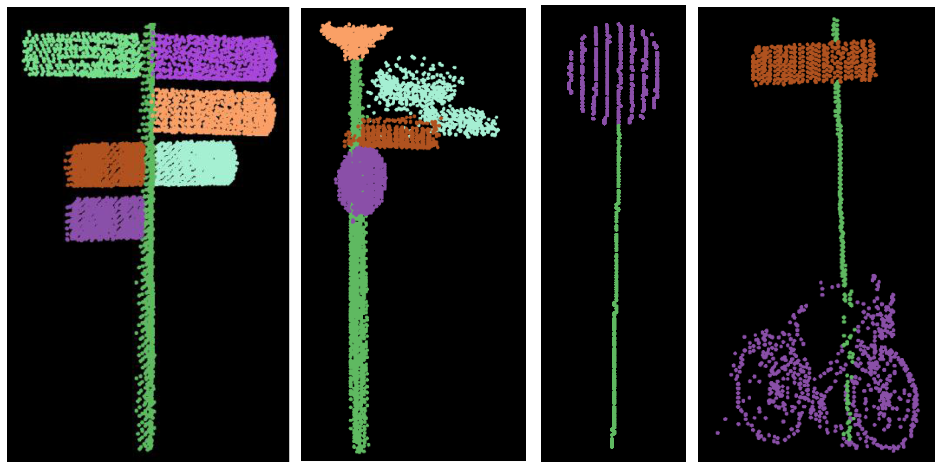
The structures and shapes of pole-like road furniture vary a lot, which makes it difficult to use a single method to extract poles. For example, in the case of many attachments connected with poles, it is difficult to directly extract poles based on their linear features. Thus, 2D point density can be adopted as a feature to extract poles. We categorized the pole-like road furniture into three typical types. The first type was road furniture with many attachments (the left image in Figure 7). The second one was road furniture with horizontal poles (the middle image in Figure 7), and the third type was normal road furniture (the right image in Figure 7). For these three different types of road furniture, three corresponding pole extraction methods were proposed.
In order to select the method to be used for pole-extraction, we first did the pre-identification to get information from the road furniture such as the length and width of its bounding box. To obtain the knowledge of the structure of the road furniture, we cut pole-like road furniture into slices and computed the width of every slice. In the previous phase, we already cut the above-ground components into slices to check if they were pole-like. We do not use the previous slicing information because the width of the previous slicing in the pole-like road furniture detection stage is rather large (e.g., 0.3 m) because it was used to connect small fragments together. In this phase, the width was set to 0.1 m. The bounding box of every individual road furniture is then calculated. The median width of the slices can be obtained by the statistics of every slice. The maximum variation of the distance between the points of one road furniture item in the XY direction can be calculated based on its bounding box.
According to the properties of road furniture calculated in the pre-processing phase, the corresponding pole extraction method was selected (Figure 8). If more than half of the pole component consists of attached components, a 2D point density-based method was utilized. This can be determined by comparing the smallest quartile width and median width. If there was a large difference, we believed that there were many components attached to the pole. Otherwise, Random Sample Consensus (RANSAC)-based line fitting was utilized if the horizontal poles were included in the road furniture. These can be detected by checking the bounding box of the piece of road furniture. If the length or width of the bounding box in the horizontal direction was larger than the threshold, the decision that this road furniture likely contained horizontal poles was made. For normal road furniture, there were more robust features to extract poles than using 2D point density features. If there were not many attachments to the road furniture, the line fitting was more robust than extracting points with high 2D point density. Consequently, we used the slice cutting based method to fit the center lines of poles and perform pole extraction. Finally, when there were no attachments to the pole, there was no need for decomposition.
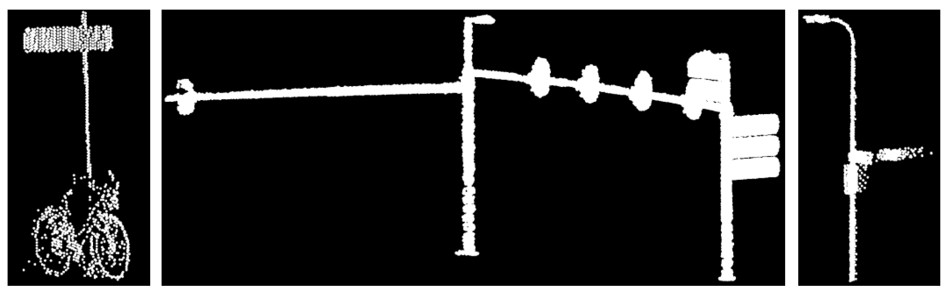
The brief explanation of these three pole extraction methods is given as follows. In the 2D point density-based method, we first calculated the 2D point density around every point. Then we used a region growing method to extract the clusters of points with high 2D point density (Figure 9a) which were recognized as poles. In the second pole extraction method, points with high linearity were first extracted by calculating the eigenvalues of every point’s neighboring points. Then the RANSAC algorithm was adopted to extract lines from these points with high linearity. Poles were extracted by detecting points within a radius to the fitted lines (Figure 9b). In the slice cutting method, we first extracted the center lines by carrying out the RANSAC algorithm with the center points of the cut slices. Similar to the second method, the poles were then extracted based on the distance between the points and fitted lines (Figure 9c). A more detailed description of these three methods is given by Li et al. (2016).
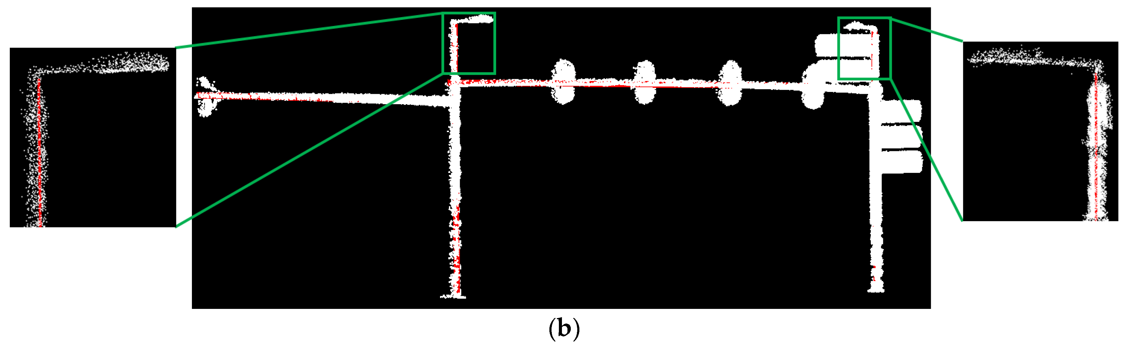
Poles extracted by the first two methods (2D point density method and RANSAC line fitting method) were often not accurate. For the 2D point density-based method, some points of attachments that are near the poles have a high 2D point density. They can thereby be categorized as poles. When points with high linearity were not extracted accurately enough, the center lines of the poles cannot be estimated correctly using the RANSAC algorithm in the second method. If a pole is inaccurately generalized to a line, this causes the imprecise extraction of the pole. For example, if the generalized center lines inclined towards the street side (Figure 10a), the part of the points that would be far away from the center lines and belong to the poles would not be extracted in this stage. To tackle these problems, pole extraction was optimized by re-estimating the center lines of the poles. Similar to the slice cutting, we cut the extracted points of poles into slices, computed their center points, and used the RANSAC algorithm to extract the lines from these center points. By doing this, poles can be extracted more accurately by using the precisely fitting center lines. The re-estimated center lines were shown in Figure 10b.
3.2.2. Decomposition into Poles and Attachments
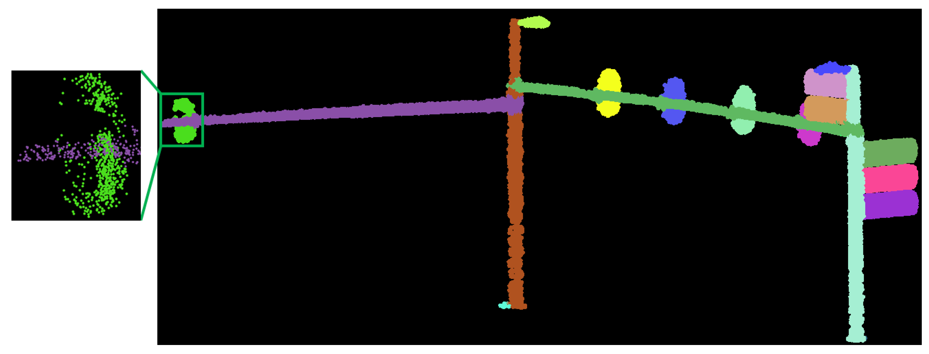
In order to separate the attachments which are connected to the poles, we removed the extracted poles and performed a connected component analysis [29]. As the components can be very close to each other, the maximum distance and the size of the nearest neighborhood should be chosen properly. Considering the distance between the scanlines and the point distribution on a single scanline, the neighborhood size cannot be very small. Otherwise, points on different scanlines would not be connected. The maximum distance between two scanlines here is 0.05 m. For a point, the number of its neighboring points was typically 10 within the distance of 0.05 m in a single scanline. Here, we set the maximum for the connected components to 0.15 m and the neighborhood size to 15 points. The separated components are as shown in Figure 11. The best method for each piece of road furniture was chosen automatically. Figure 11a shows the partitioning of the remainder of points which were obtained from a 2D point density-based pole extraction method. Pole extraction in Figure 11b uses the RANSAC line fitting method and pole extraction in Figure 11c,d utilized the slice cutting based method.
Because of occlusion, low point density, and noisy points, it is sometimes difficult to connect all the points that belong to the same attachment by leveraging the parameters of the aforementioned connected component analysis. Examples are marked in Figure 11. To address this problem, we defined a set of generic rules to split and merge the components. We first performed merging rules for the components for horizontal poles. Then the components connected to vertical poles were analyzed to see whether they could be merged or split. Then, the detached components were checked on whether they could be merged with their nearby components.
As shown in the red circle of Figure 11b, one component attached to a horizontal pole can be separated into two parts during the connected component analysis. If two components were attached to the same horizontal pole and their positions overlap in XY-plane, these two components should be merged. The merging analysis of the horizontal pole attached components was repeated until no such components were found. Figure 12 shows the merged components after applying the merging rule.
Another situation was that the attachments might be connected to each other because of noisy points or imprecise pole extraction. An example is shown in the Figure 11c. In this situation, we increase the width of the pole extraction. If one component can be split into two parts and they are not at the same height, this component was split into two parts. This method is similar to erosion followed by dilation.
Suppose is a component which is attached to vertical poles when the width is set to for pole extraction. We increased —where is the width of the cut slice —and performed a connected component analysis. Once becomes the two components— and —and they are not at the same height, they should be separated into two parts. This operation will continue until the increment of reaches a predefined value. In this paper, it is empirically set to 0.15 m for the splitting analysis.
There are single attachments which might be separated into two parts (Figure 11a). This case occurs when the distance for connection is not large enough during the connected component analysis. In this case, we conducted a merging analysis. We continued increasing the width of the pole extraction to . Here, we set to be the normal size of traffic signs, for example, 0.5 m. Once the two components and are wrapped by their connected vertical pole and once the two components are in the same height, the connection line of their center points comes very near to the pole line. Then they should be merged together. The merging analysis will be iterated until no components can be merged. The components were split and merged as shown in the red circle of Figure 13.
Components that were not connected to poles (Figure 11d) were described as detached components because of the low point density or occlusion. It is assumed that if one detached component and an attachment were at the same height, on the same side, and their connection line was very close to this pole, they should be one component and merged together. Then, this merged component was added to continue with the detached components merging analysis. The detached components were merged as illustrated in Figure 14.
3.3. Final Detection of Pole-Like Road Furniture
The results of the decomposition were imported as it is feedback for the road furniture detection stage. If there was no pole extracted from a road furniture item such as the pillars of buildings, this road furniture item would not be labeled as pole-like. For example, the pillars of buildings can be detected as a pole-like road furniture item at the detection stage. When such a pillar is decomposed by using RANSAC line fitting, this pillar will probably not be extracted because the percentage of points which belong to the pole is low when there are many points with a high linearity from the edges of façades or fragments.
3.4. Road Furniture Decomposition Evaluation
In this section, an approach was presented to evaluate the accuracy of the decomposition. Based on their spatial relations, the components of pole-like road furniture were manually labeled. For example, street signs can be manually labeled as “pole and attachments”, as shown in Figure 15.
In order to assess the results of the decomposition, we used a two-level evaluation method. One is point-based evaluation and the other one is a component-based evaluation. We used completeness and correctness to quantify the evaluation.
In the point-based evaluation, we first selected the corresponding true positive points of the manually labeled ground truth component. We matched the corresponding decomposition result and every ground truth component by selecting the largest decomposed component in this ground truth component. The true positive points in an attachment are the points belonging to both this attachment and its corresponding manually labeled attachment. Then the completeness of every component was computed as the ratio of the number of points of the largest segment in this component to the number of points of this component, . is the number of correctly decomposed points in the manually labeled components, is the number of incorrectly decomposed points in the manually labeled components. For example, in Figure 16, the true positive component of the streetlight head is the decomposed component which is marked by the red circle 1 in the left figure. Thus, the completeness of this component can be computed as the ratio of the number of points which are in the overlap of the component labeled with the red circle 1 in the left figure and the component labeled with green circle 1 in the right figure, to the number of points of the component labeled with the green circle 1 in the right figure.
The correctness of a separated attachment is the number of true positive points divided by the number of points of this separated attachment. For example, in Figure 16, the correctness of this component is computed as the ratio of the number of points which are the overlap of the component labeled with the red circle 1 in the left figure and the component labeled with the green circle 1 in the right figure, to the number of points of the component labeled with a green circle 1 in the right figure. . is the number of incorrectly decomposed points in the components produced by our algorithm. Those points which are labeled with the green circle 1 in the right figure are included as well in the segment which is labeled with the red circle 1 in the left figure.
In the component-based evaluation, the largest segment in every manually labeled ground truth component was selected as the corresponding segment of this component. Then we calculated the completeness and correctness of every component by using point-based evaluation. If the completeness was lower than the threshold , this component was labeled as over-decomposed. If the correctness was lower than the threshold , this component was labeled as under- decomposed. Otherwise, this component was an applicable decomposed component. Both and were defined to be 0.6. For example, in the left image of Figure 16, component 2 labeled with a green circle is under-decomposed with low correctness. In contrast, component 3 is over-decomposed with low completeness.
4. Study Area and Experimental Result
To test the performance of the proposed framework, two datasets—one in Enschede and one in Paris—are chosen. The Enschede dataset was used as a test case because there are many types of road furniture and it is a typical Dutch city. The Paris dataset was a benchmark dataset and Paris is a French city. The shapes of the road furniture in these two test sites are different because they are from two different countries.
The test of the presented framework on the Enschede dataset is given in Section 4.1 and Section 4.2 gives the experimental results of the Paris dataset. The analysis of the results is explained in the corresponding sections. In Section 4.3, the limitations and applicability are analyzed.
4.1. Enschede
4.1.1. Test Site
This dataset was collected in Enschede, a medium-sized city located in the east part of the Netherlands. It was acquired by TopScan GmbH in December 2008. The Optech LYNX mobile mapping system was used to capture the laser scanning data. This system consists of two rotating laser scanners, which were mounted on the backside of a moving vehicle. Their directions are perpendicular and make a 45° angle with the driving direction. The frequency of both scanners was 100 kHz. The platform was driven at a maximum speed of 50 km/h. In this dataset, the coordinates plus two attributes—the pulse count and reflectance strength—are available.
The Enschede MLS data are about 1.25 km long, consisting of 19,945,716 points and 151 pieces of road furniture. The point density ranges from 35 points per square meter to 350 points per square meter. The test area was partitioned into 25 blocks along the trajectory line, with each block 50 m long and 40 m wide.
4.1.2. Results
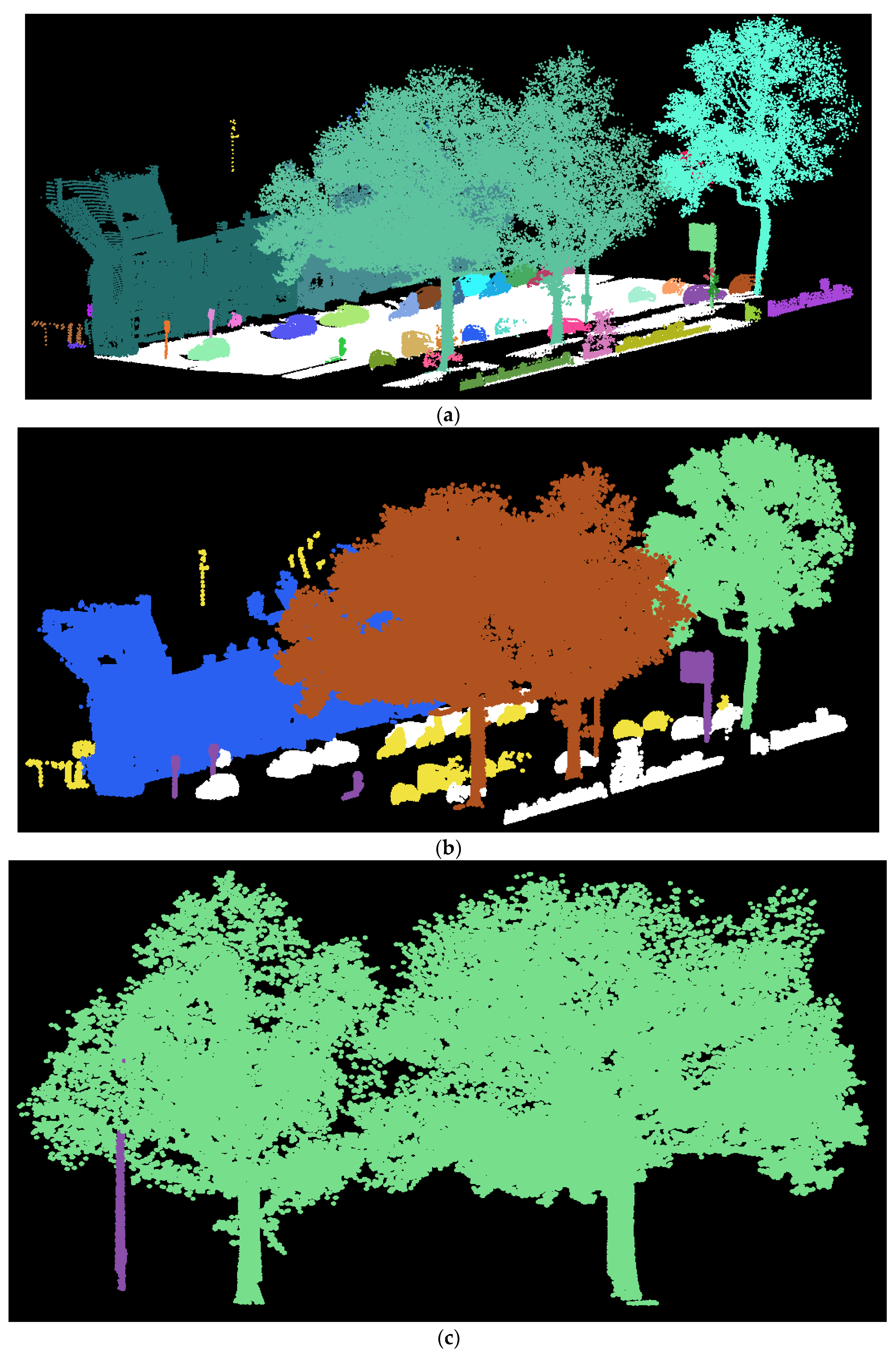
The road furniture detection of a single road part in the Enschede dataset is as shown in Figure 17. The height difference was firstly estimated for every point in this road part. The height difference threshold between all nearby points within a certain neighborhood in order to filter ground points was set to 0.15 m. The neighboring size for the height difference calculation was set to be high (for example, 100) due to the high point density of the road surfaces. Then points with a small height difference were categorized as ground points (Figure 17a) and removed. The filtered ground points were colored white. Subsequently, the above-ground components (Figure 17a) were produced by removing the ground points and the connected component analysis. The dynamic objects were labeled (Figure 17b) and eliminated from the above-ground components afterward. Most of them were cycling bicycles, pedestrians, and moving vehicles. Because of the angles and occlusions, several objects behind building façades were scanned by only one laser scanner. This leads to these objects behind building façades being labeled as dynamic objects. Although this was incorrect, it does not affect our results because we would like to eliminate these objects behind the façades anyway. Then the façades were recognized (Figure 17b). More detailed information on this process was explained in Section 3.1.2. At the end of the detection phase, the slice-based poles were analyzed. Vegetation, pole-like road furniture, and road furniture connected with vegetation were detected as in Figure 17b. Due to the close proximity, some vegetation connected with road furniture was also detected. Two trees connected with one streetlight were colored as brown in this figure. Their separation was as shown in Figure 17c. The detected pole-like road furniture were colored in purple. The detected pole-like road furniture were as shown in Figure 18a. False positively detected road furniture inside buildings were excluded after the occlusion analysis, shown in Figure 18b.
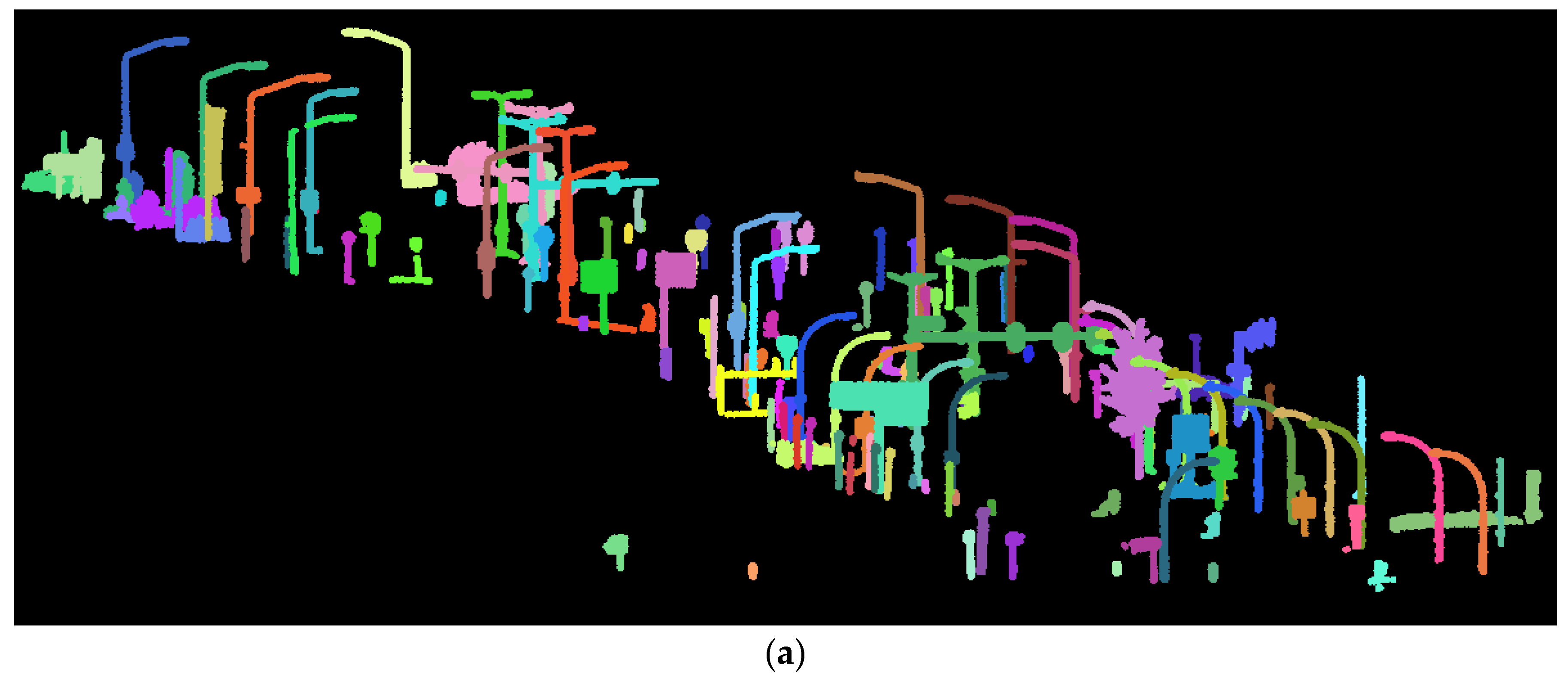
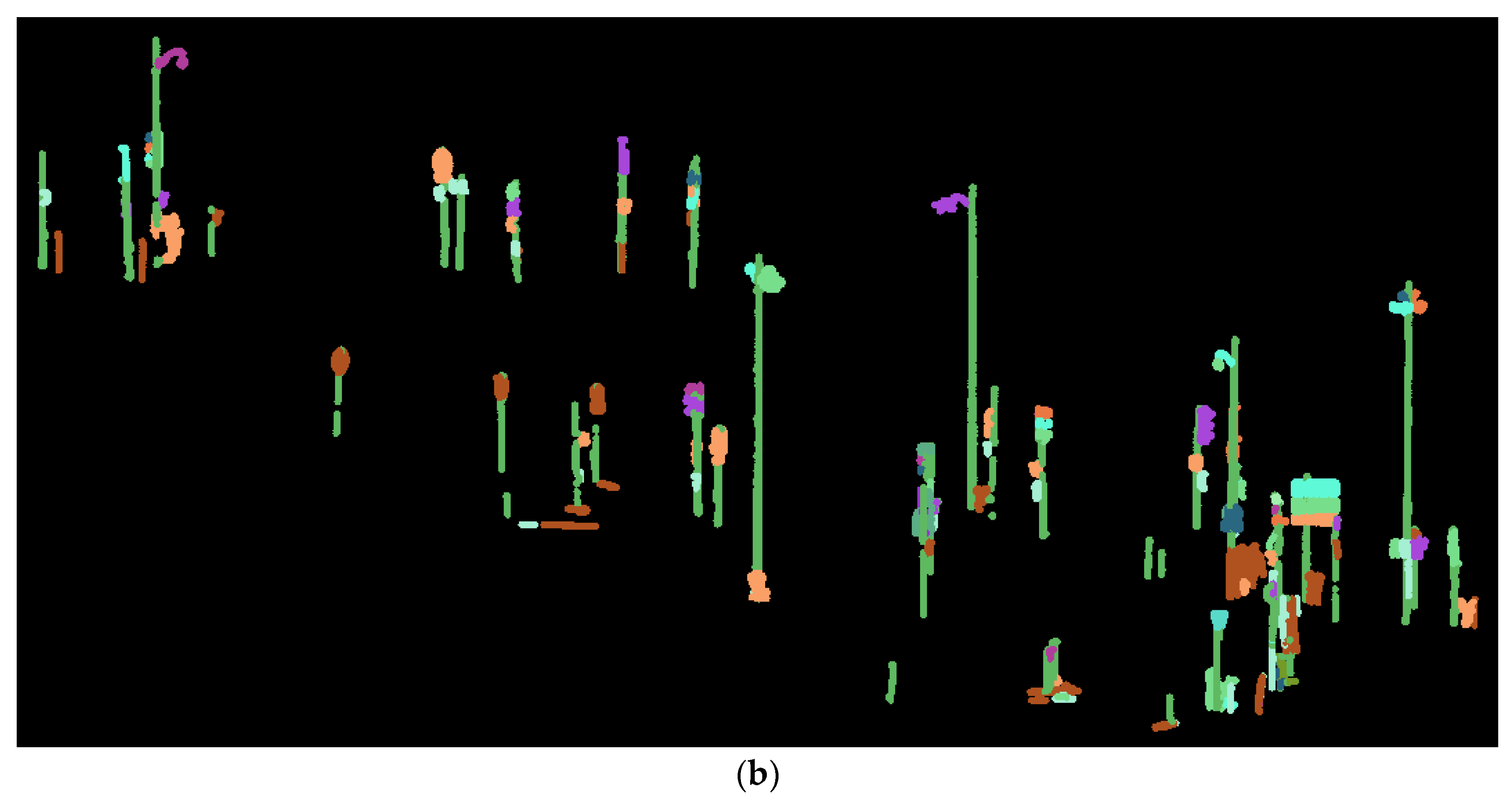
At the stage of decomposition, particular attention was paid to complex structures rather than bare poles. Therefore, we removed the bare poles and only complex structural pole-like road furniture were identified as the input for the decomposition test. In this dataset, 115 pole-like road furniture were detected, given in Figure 19a. The final results of the pole-like road furniture decomposition can be found in Figure 19b.
4.1.3. Performance Analysis and Parametric Sensitivity Analysis
For the evaluation of pole-like road furniture detection, we manually inspected every detected pole-like road furniture. The completeness and correctness of pole-like road furniture detection are as shown in Table 1. The correctness is 96.0% and the completeness is 94.7%. In total, 149 pole-like road furniture items were detected, 6 of which were incorrectly recognized. Among these false positive detected entities, there were small garbage boxes and thin trees. Small garbage boxes were partially scanned and they were similar to short poles such as road piles. Thin trees without many branches and leaves were also easily recognized as pole-like road furniture. This was because it was difficult to distinguish them from pole-like road furniture only from the structure information. Future research could be to investigate the color information in combination with the point cloud. Two pole-like road furniture items were not identified because of the noisy points and low point density. Four traffic boards are identified as pole-like road furniture. Although their structure is obviously non-pole-like, they can still be categorized as road furniture because of their salient traffic functionalities. Nevertheless, we strictly consider the detected traffic boards as negative results.
The accuracy evaluation of the decomposition of the pole-like road furniture from the Enschede dataset is given in Table 2. The completeness is above 79.5% and the correctness is 92.3%. Compared to our previous work in which pole extraction optimization and rules were not applied, the performance improved significantly in the point-wise evaluation. Due to the high point density of this dataset, the components were already well-separated in the point level. The ratio of the correctly decomposed components increases from 72.2% to 79.5%, which proves the improvement of the decomposition after the addition of pole extraction optimization and rules for the decomposition part.
In order to set proper parameters, we chose one block which contained 22 pieces of road furniture to train the parameter settings. In the detection phase, the threshold of the maximum diameter of pole-like slices was obtained by using a grid search. The optimal threshold was 0.50 m. Then we used the trained parameter to detect pole-like road furniture. In the decomposition phase, we also use a grid search to obtain the optimal ratio of the width of every slice for pole extraction. A set of parameters {0.25, 0.5, 0.75, 1.0, 1.25, 1.50} was tested on the sampling data. A value of 0.75 proved to be the optimal parameter.
4.2. Paris
4.2.1. Test Site
The test data of Paris (France) was captured in January 2013 by a Stereopolis II system, an MLS system developed by the French National Mapping Agency IGN. This is the IQmulus & TerraMobilita Contest dataset [39]. This dataset contains MLS data from a dense urban environment, composed of 300 million points, covering approximately 10 km. In addition, it is an accessible benchmark dataset. In this dataset, there are two available attributes: reflectance and pulse count information.
The Paris MLS data was acquired in 10 zones. Compared with other zones, most road furniture was in zone 7. For this reason, it was selected as the test data zone. This test area is about 0.43 km long, consisting of 13,776,061 points and containing 132 pieces of road furniture. The test area was partitioned into 13 blocks along the trajectory line. We designed each block to be 40 m long and 30 m wide because the Paris streets are fairly narrow. The point density ranged from 72 points per square meter to 500 points per square meter. Compared with the Enschede dataset, the point distribution of the road furniture in the Paris dataset was quite uneven. This was because the scanning pattern was different. The Paris dataset was collected by only one laser scanner.
4.2.2. Results
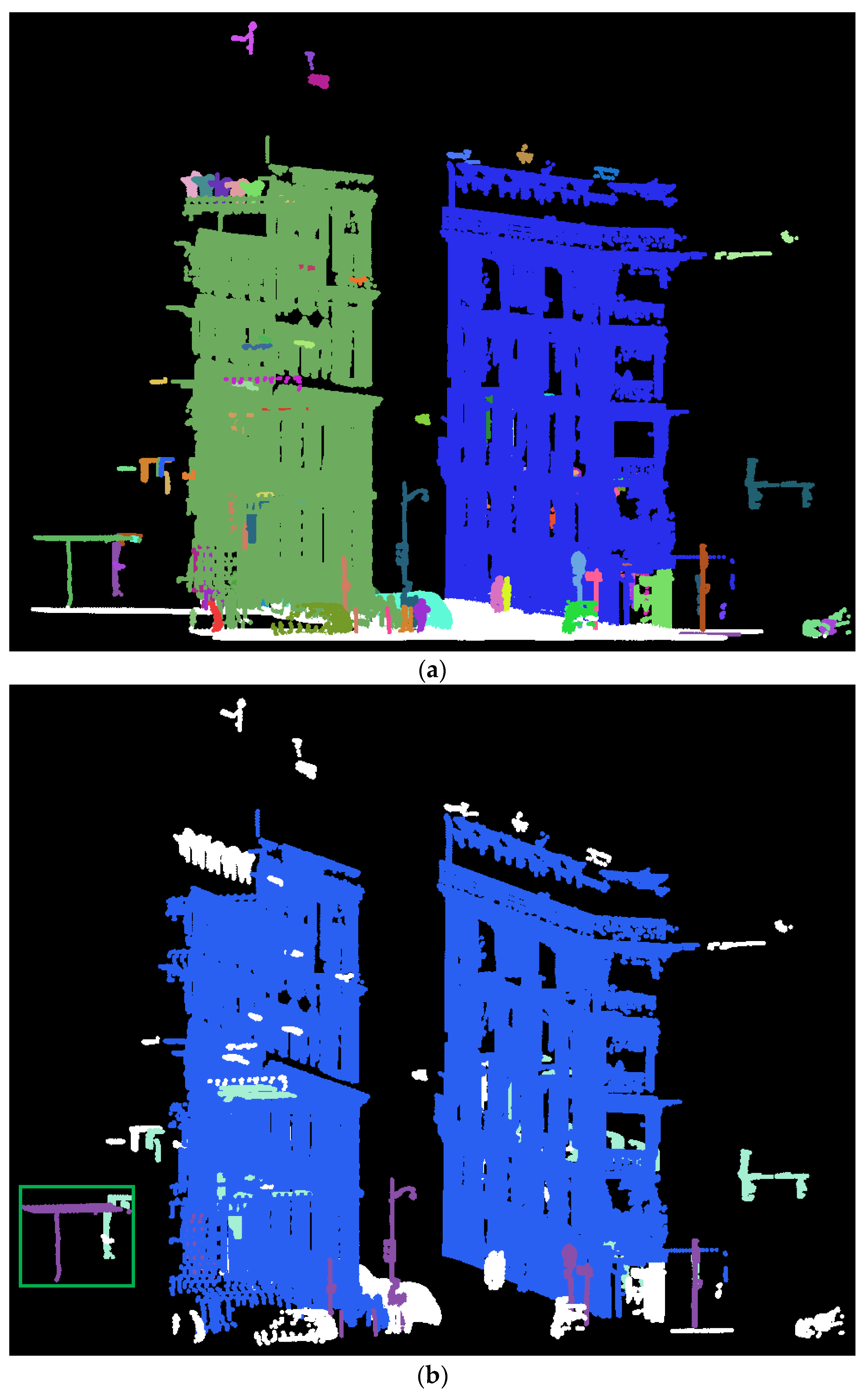
The original point cloud of one road part was as shown in Figure 20. The detected ground points, above-ground components, and façade points were as shown in Figure 20a. The detected pole-like road furniture before and after occlusion analysis are illustrated in Figure 20b,c.
Some entities behind the façades were detected as vegetation. The reason for this was that these objects were collected with multiple echo count information when the laser pulses passed through the windows and hit objects behind the windows. As this dataset was captured by using only one laser scanner, dynamic objects were not detectable by our framework.
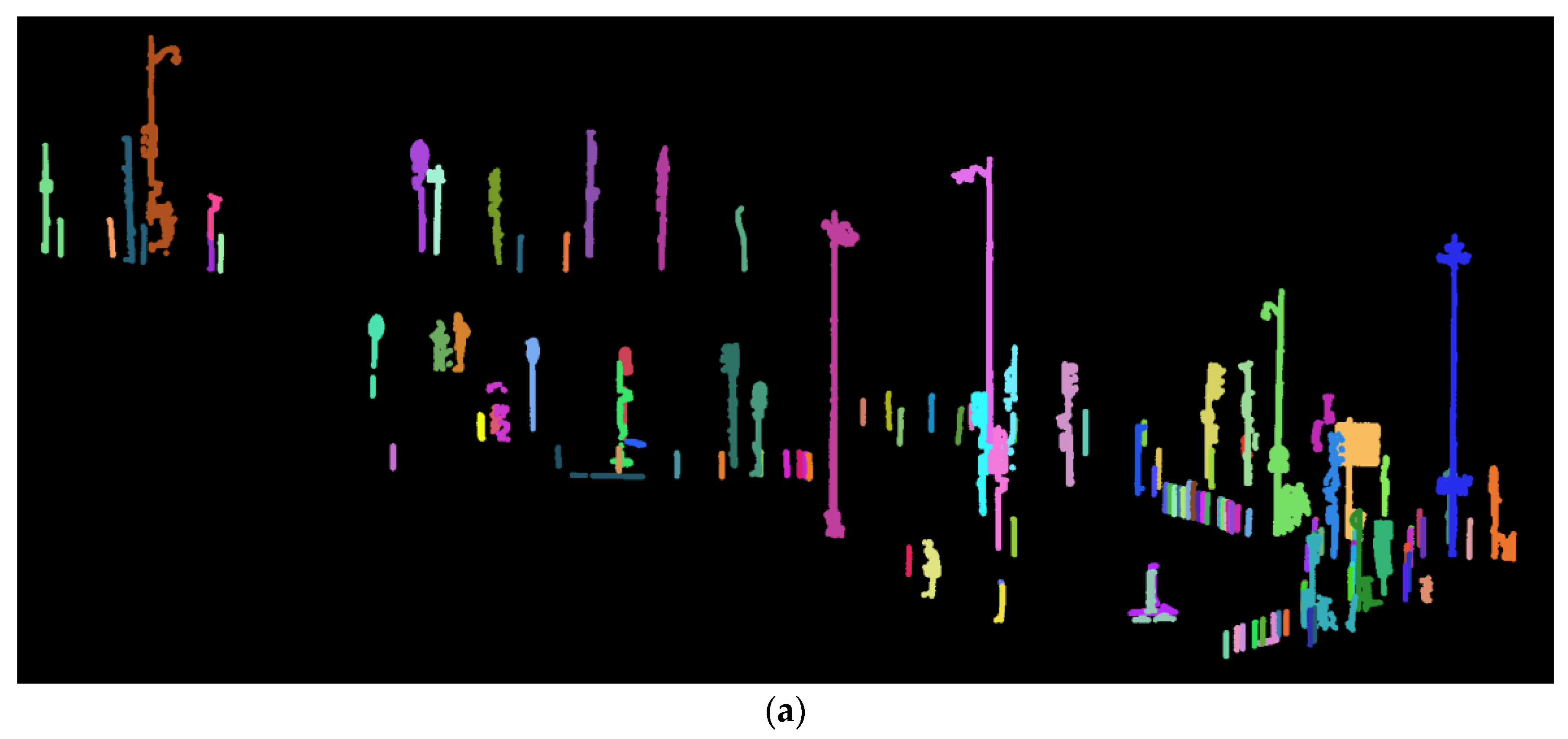
In this dataset, 41 pole-like road furniture items were identified as poles with attachments (see Figure 21a), and 97 were identified as bare poles. The detected poles with attachments were used to quantify the decomposition results. The pole-like road furniture decomposition result was as depicted in Figure 21b.
4.2.3. Performance Analysis and Parametric Sensitivity Analysis
By means of visual inspection, the performance of pole-like road furniture detection in the Paris dataset was evaluated. Table 3 shows that the correctness was 91.3% and the completeness was 95.4% in this dataset. In total, there were 138 pole-like road furniture items detected, 12 of which were incorrectly recognized. Among these false positive detected entities, most of them were pedestrians and entities whose point clouds were partially acquired. Pedestrians are similar to pole-like road furniture, especially in a noisy dataset. Another factor is that some road objects like fences were only partially scanned and are similar to pole-like road furniture in appearance. It is still a challenging task to distinguish them. Six pole-like road furniture items were not identified because of the low point density. Similar to the Enschede dataset, we also selected the optimal parameters by using a grid search in the Paris dataset. The optimal threshold of the maximum diameter of the pole-like slices was determined to be 0.30 m. The optimal ratio of the width of every slice for pole extraction was 0.50.
The performance of our previous work and the current framework is illustrated in Table 4. Compared with the Enschede dataset, the quality of the Paris dataset is lower. For example, in the Paris dataset, the point distribution was uneven because of the usage of a single scanner. Because the decomposition method required a high-quality point cloud, the performance of our previous work tested on the Paris dataset was not satisfying. As shown in Table 4, the results of the decomposition were obtained by our previous work [29] in which we did not utilize pole extraction optimization and rules. With the addition of pole extraction optimization and rules in the decomposition part, the completeness was improved to be above 80%, the correctness was improved to be 92.6%, and the rate of correctly decomposed components was enhanced to 72.0%. The results prove the effectiveness of the proposed framework.
4.3. Discussion
Our carried out research aimed to decompose pole-like road furniture into poles and attachments based on their spatial relations such as connectivity. In this study, we developed a new framework to detect and decompose pole-like road furniture automatically. As our results show, pole-like road furniture were detected accurately and automatically. Approximate 90% of pole-like road furniture items were detected and more than 90% was correctly detected in both test sites. The correctness of road furniture detection was 92.3% and completeness was 83.3% in Cabo et al. [17]. In Yang et al. [32], their achieved correctness and completeness of road furniture detection was higher than 90.0%. The average completeness of our framework is 95.0% and the average correctness is 93.6%. Our framework is competitive with the current state of the art in the field of pole-like road furniture detection. The completeness of decomposition was above 80% and the correctness of decomposition was above 90% in both experimental areas. Besides that, we introduced an automatic method to evaluate the accuracy of the decomposition instead of the visual inspection mentioned in our previous work.
A significant advantage of this framework is the adoption of occlusion analysis. All pole-like objects inside buildings were eliminated in the Enschede test case, and only four pole-like objects inside buildings were not filtered out in the Paris test site. These four objects were located close to building façades whose normal direction was almost parallel to the trajectory direction. Our occlusion analysis was not able to cope with such situations. The pole-extraction optimization, defined merging, and splitting rules also improved the performance of the decomposition. It enhances the ratio of correctly decomposed components by 7.3% in the Enschede test site and 18.4% in the Paris test area. Some well-decomposed road furniture is shown in Figure 22.
Even though the accuracy of pole-like road furniture detection is already high, some problems still remain. In both of the two test sites, small booths supported by pillars were recognize as pole-like road furniture. These booths have pillars whose appearance is very similar to poles. The detection algorithm was not good enough to discriminate the difference. Therefore, additional structural relations will be added later to address this problem. In the slicing-based pole-like road furniture detection step, trees connected to the pole-like road furniture were detected. We have yet been unable to thoroughly separate them (Figure 17d).
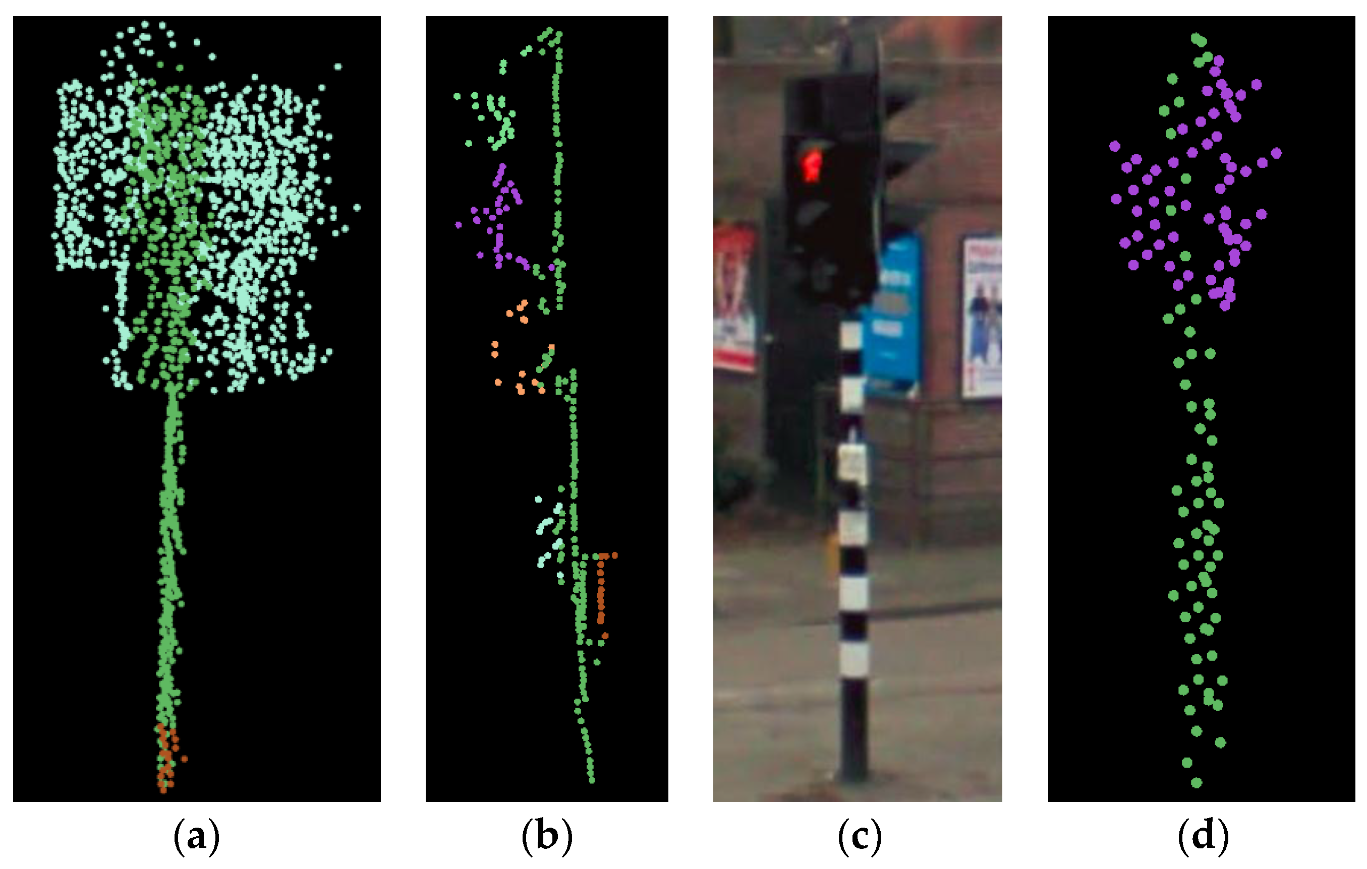
The remaining problems with decomposition are divided into two types. The first one is the problem with the data itself. Specifically, it involves point density, point distribution, and noisy points. In Figure 23a, the two connected traffic signs should have been separated. If there are many noisy points around one road furniture item, it is even harder to separate these attached components by visual interpretation. Under such circumstances, our decomposition algorithm does not work. If the point density is extremely low, points cannot form an individual component. For example, in the Paris dataset, a few traffic lights were documented by several points, which led to the fragmented unstructured components during the decomposition (Figure 23b). In contrast, most of the traffic signs were decomposed as individual components owing to their adequate point density. Therefore, the point density cannot be very low. The point spacing between points in the trajectory direction is normally higher than 0.05 m. The point spacing was about 0.02 m within the scanlines. The point spacing in these two directions was different. The second problem originates from the scene. Currently, curved poles cannot be extracted as the assumption is that pole-like road furniture contains straight poles. Beside this, pedestrian-oriented traffic lights (Figure 23c) which consist of traffic light heads connected with each other cannot be decomposed correctly (Figure 23d).
5. Conclusions
In this paper, we proposed a new framework to detect pole-like road furniture and decompose them into different components based on their logical relations. This innovative framework is tested in two test sites. After being processed by our new framework, the road furniture were detected and interpreted by logical relations, which can be used for precise semantics labeling. This proposed framework can be potentially used for high defined 3D mapping. In this framework, we improved road furniture detection by combining dynamic objects removal, pole slicing, and occlusion analysis. The completeness and correctness values of the pole-like road furniture detection were higher than 90% in both the Enschede dataset and the Paris dataset. The main contribution was the decomposition of the road furniture and its evaluation. Compared with our previous work, the current framework is completely automatic and the performance of decomposition has been improved by applying defined rules.
The next stage of our work will focus on the classification of decomposed road furniture. Even though logically separated components were obtained, the meaning of every component has not been assigned yet. Therefore, in order to make use of the components for further applications such as mapping, these components will be semantically labeled based on their features.
In our research, road furniture items have been decomposed into components by using mere geometric features. Color information has also been beneficial to the detection and decomposition. Many techniques on image semantics labeling such as the convolutional neural network can be applied to our research. 2D image data were also captured by two cameras mounted on a moving vehicle. The clear detection, decomposition, and classification of road furniture could benefit from the color information given by the 3D point cloud.
Acknowledgments
The research is supported by Chinese Scholarship Council. The authors want to thank Marco Oesting for the English editing.
Author Contributions
Fashuai Li designed the algorithms as described in this paper, and was responsible for the main organization and writing of the paper. All the work was done under the supervision of Sander Oude Elberink and George Vosselman.
Conflicts of Interest
The authors declare no conflicts of interest.
References
- World Health Organization. In Global Status Report on Road Safety 2015; World Health Organization: Geneva, Switzerland, 2015.
- Adesiyun, A.; Avenoso, A.; Dionelis, K.; Cela, L.; Nicodème, C.; Goger, T.; Polidori, C. Effective and coordinated road infrastructures safety operations. Transp. Res. Proced. 2016, 14, 3304–3311. [Google Scholar] [CrossRef]
- Bauer, R.; Steiner, M.; Kühnelt-Leddhin, A.; Lyons, R.; Turner, S.; Walters, W.; Larsen, B.; Valkenberg, H.; Bejko, D.; Ellsaesser, G.; et al. Scope and patterns of under-reporting of vulnerable road users in official road accident statistics Monica Steiner. Eur. J. Public Health 2017, 27 (Suppl. 3). [Google Scholar] [CrossRef]
- U.S. Department of Transportation Federal Highway Administration. Available online: http://safety.fhwa.dot.gov/tools/data_tools/mirereport/ (accessed on 28 January 2018).
- Soilán, M.; Riveiro, B.; Sánchez-Rodríguez, A.; Arias, P. Safety assessment on pedestrian crossing environments using MLS data. Accid. Anal. Prev. 2018, 111, 328–337. [Google Scholar] [CrossRef] [PubMed]
- Ibañez-Guzman, J.; Laugier, C.; Yoder, J.D.; Thrun, S. Autonomous driving: Context and state-of-the-art. In Handbook of Intelligent Vehicles; Eskandarian, A., Ed.; Springer: London, UK, 2012; pp. 1271–1310. [Google Scholar]
- Jaakkola, A.; Hyyppä, J.; Hyyppä, H.; Kukko, A. Retrieval algorithms for road surface modelling using laser-based mobile mapping. Sensors 2008, 8, 5238–5249. [Google Scholar] [CrossRef] [PubMed]
- Oude Elberink, S.; Vosselman, G. 3D information extraction from laser point clouds covering complex road junctions. Photogramm. Rec. 2009, 24, 23–36. [Google Scholar] [CrossRef]
- Zhang, W. Lidar-based road and road-edge detection. In Proceedings of the IEEE Intelligent Vehicles Symposium (IV), San Diego, CA, USA, 21–24 June 2010. [Google Scholar]
- Zhou, L.; Vosselman, G. Mapping curbstones in airborne and mobile laser scanning data. Int. J. Appl. Earth Obs. Geoinf. 2012, 18, 293–304. [Google Scholar] [CrossRef]
- Oude Elberink, S.; Khoshelhama, K.; Arastouniab, M.; Benitoc, D.D. Rail track detection and modelling in mobile laser scanner data. ISPRS Ann. Photogramm. Remote Sens. Spat. Inf. Sci. 2013, 2, 223–228. [Google Scholar] [CrossRef]
- Yang, B.; Fang, L. Automated extraction of 3-D railway tracks from mobile laser scanning point clouds. IEEE J. Sel. Top. Appl. Earth Obs. Remote Sens. 2014, 7, 4750–4761. [Google Scholar] [CrossRef]
- Lehtomäki, M.; Jaakkola, A.; Hyyppä, J.; Kukko, A.; Kaartinen, H. Detection of Vertical Pole-Like Objects in a Road Environment Using Vehicle-Based Laser Scanning Data. Remote Sens. 2010, 2, 641–664. [Google Scholar] [CrossRef]
- Pu, S.; Rutzinger, M.; Vosselman, G.; Oude Elberink, S. Recognizing basic structures from mobile laser scanning data for road inventory studies. ISPRS J. Photogramm. Remote Sens. 2011, 66, S28–S39. [Google Scholar] [CrossRef]
- El-Halawanya, S.I.; Lichti, D.D. Detecting road poles from mobile terrestrial laser scanning data. GISci. Remote Sens. 2013, 50, 704–722. [Google Scholar]
- Li, D.; Oude Elberink, S. Optimizing detection of road furniture (pole-like objects) in mobile laser scanner data. ISPRS Ann. Photogramm. Remote Sens. Spat. Inf. Sci. 2013, 1, 163–168. [Google Scholar] [CrossRef]
- Cabo, C.; Ordoñez, C.; García-Cortés, S.; Martínez, J. An algorithm for automatic detection of pole-like street furniture objects from mobile laser scanner point clouds. ISPRS J. Photogramm. Remote Sens. 2014, 87, 47–56. [Google Scholar] [CrossRef]
- Huang, J.; You, S. Pole-like object detection and classification from urban point clouds. In Proceedings of the IEEE International Conference on Robotics and Automation, Seattle, WA, USA, 26–30 May 2015. [Google Scholar]
- Fukano, K.; Masuda, H. Detection and classification of pole-like objects from mobile mapping data. ISPRS Ann. Photogramm. Remote Sens. Spat. Inf. Sci. 2015, 2, 57–64. [Google Scholar] [CrossRef]
- Yang, B.; Dong, Z.; Zhao, G.; Dai, W. Hierarchical extraction of urban objects from mobile laser scanning data. ISPRS J. Photogramm. Remote Sens. 2015, 99, 45–57. [Google Scholar] [CrossRef]
- Yu, Y.; Li, J.; Guan, H.; Wang, C.; Yu, J. Semiautomated extraction of street light poles from mobile lidar point-clouds. IEEE Trans. Geosci. Remote Sens. 2015, 53, 1374–1386. [Google Scholar] [CrossRef]
- Puttonen, E.; Jaakkola, A.; Litkey, P.; Hyyppä, J. Tree classification with fused mobile laser scanning and hyperspectral data. Sensors 2011, 11, 5158–5182. [Google Scholar] [CrossRef] [PubMed]
- Rutzinger, M.; Höfle, B.; Oude Elbernik, S.; Vosselman, G. Feasibility of facade extraction from mobile laser scanning data. Photogramm. Fernerkund. Geoinf. 2011, 3, 97–107. [Google Scholar] [CrossRef]
- Demantké, J.; Vallet, B.; Paparoditis, N. Streamed vertical rectangle detection in terrestrial laser scans for facade database production. ISPRS Ann. Photogramm. Remote Sens. Spat. Inf. Sci. 2012, 1, 99–104. [Google Scholar] [CrossRef]
- Yang, B.; Dong, Z. A shape-based segmentation method for mobile laser scanning point clouds. ISPRS J. Photogramm. Remote Sens. 2013, 81, 19–30. [Google Scholar] [CrossRef]
- Niemeyer, J.; Rottensteiner, F.; Soergel, U. Contextual classification of lidar data and building object detection in urban areas. ISPRS J. Photogramm. Remote Sens. 2014, 87, 152–165. [Google Scholar] [CrossRef]
- Riegl. 2017. Available online: http://www.riegl.com/uploads/tx_pxpriegldownloads/RIEGL_VMX-1HA_at-a-glance_2017-05-04.pdf (accessed on 28 January 2018).
- Nurunnabi, A.; Belton, D.; West, G. Robust segmentation for large volumes of laser scanning three-dimensional point cloud data. IEEE Trans. Geosci. Remote Sens. 2016, 54, 4790–4805. [Google Scholar] [CrossRef]
- Li, F.; Oude Elberink, S.; Vosselman, G. Pole-like street furniture decomposition in mobile laser scanning data. ISPRS Ann. Photogramm. Remote Sens. Spat. Inf. Sci. 2016, 3, 193–200. [Google Scholar] [CrossRef]
- Golovinskiy, A.; Kim, V.G.; Funkhouser, T. Shape-based recognition of 3D point clouds in urban environments. In Proceedings of the 12th International Conference on Computer Vision (ICCV09), Kyoto, Japan, 27 September–4 October 2009. [Google Scholar]
- Munoz, D.; Vandapel, N.; Hebert, M. Directional associative markov network for 3D point cloud classification. In Proceedings of the Fourth International Symposium on 3D Data Processing, Visualization and Transmission, Atlanta, GA, USA, 18 June 2008. [Google Scholar]
- Yang, B.; Liu, Y.; Liang, F.; Dong, Z. Using mobile laser scanning data for features extraction of high accuracy driving maps. Int. Arch. Photogramm. Remote Sens. Spat. Inf. Sci. 2016, 41, 433–439. [Google Scholar] [CrossRef]
- Huang, J.; You, S. Point cloud labeling using 3d convolutional neural network. In Proceedings of the International Conference on Pattern Recognition, Cancun, Mexico, 4–8 December 2016. [Google Scholar]
- Soilán, M.; Riveiro, B.; Martínez-Sánchez, J.; Arias, P. Traffic sign detection in MLS acquired point clouds for geometric and image-based semantic inventory. ISPRS J. Photogramm. Remote Sens. 2016, 114, 92–101. [Google Scholar] [CrossRef]
- Hackel, T.; Wegner, J.D.; Schindler, K. Fast semantic segmentation of 3d point clouds with strongly varying density. ISPRS Ann. Photogramm. Remote Sens. Spat. Inf. Sci. 2016, 3, 177–184. [Google Scholar] [CrossRef]
- Yu, Y.; Li, J.; Wen, C.; Guan, H.; Luo, H.; Wang, C. Bag-of-visual-phrases and hierarchical deep models for traffic sign detection and recognition in mobile laser scanning data. ISPRS J. Photogramm. Remote Sens. 2016, 113, 106–123. [Google Scholar] [CrossRef]
- Oude Elberink, S.; Kemboi, B. User-assisted object detection by segment based similarity measures in mobile laser scanner data. Int. Arch. Photogramm. Remote Sens. Spat. Inf. Sci. 2014, 40, 239–246. [Google Scholar] [CrossRef]
- Vosselman, G.; Maas, H.G. (Eds.) Airborne and Terrestrial Laser Scanning; Whittles Publishing: Caithness, UK, 2010. [Google Scholar]
- Vallet, B.; Brédif, M.; Serna, A.; Marcotegui, B.; Paparoditis, N. TerraMobilita/iQmulus urban point cloud analysis benchmark. Comput. Graph. 2015, 49, 126–133. [Google Scholar] [CrossRef] [Green Version]
Figure 1.
The workflow of our framework.
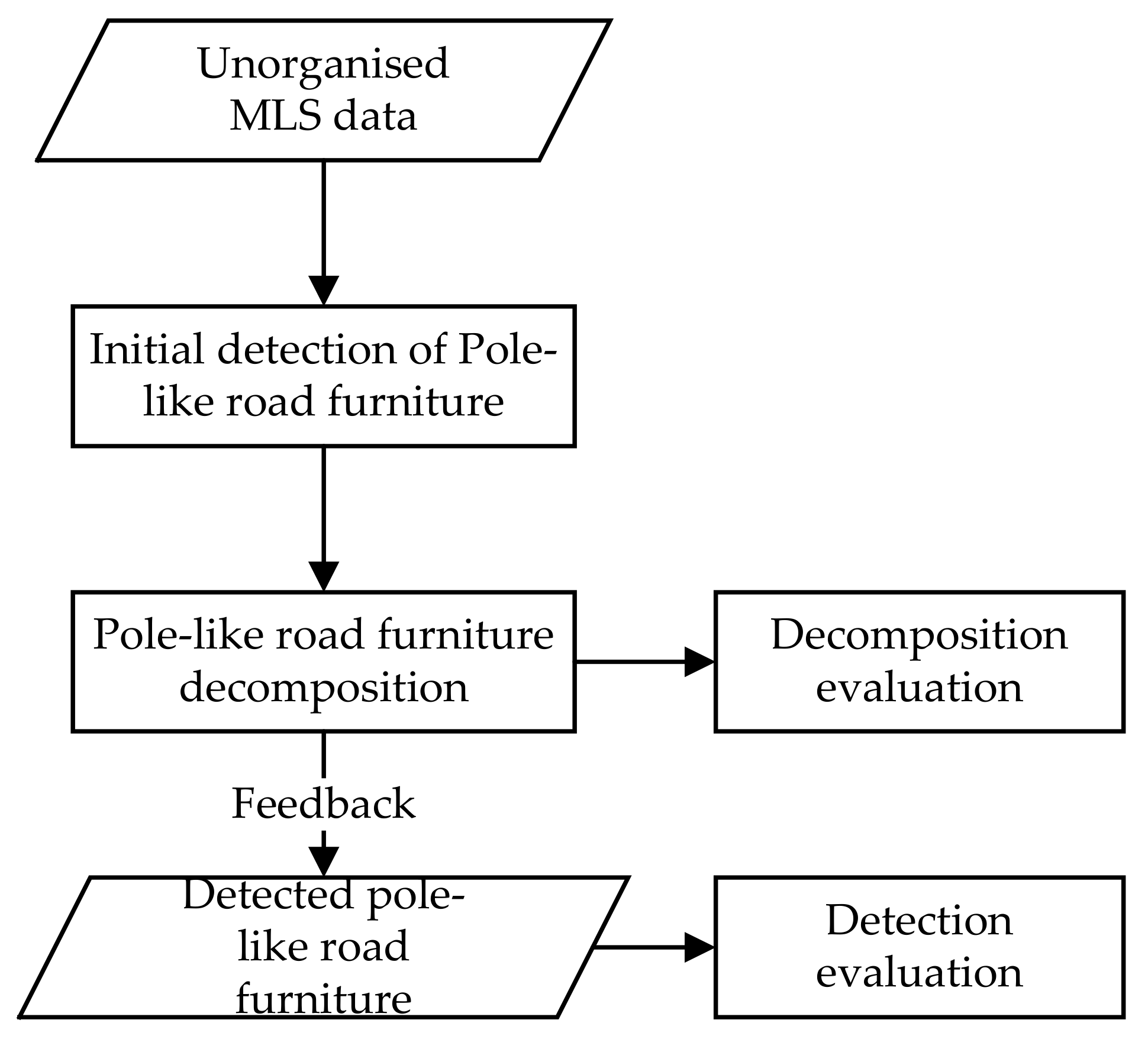
Figure 2.
The workflow of the initial road furniture detection.

Figure 3.
The workflow of detecting pole-like road furniture.

Figure 4.
The slice-based detection of pole-like road furniture.

Figure 5.
Occlusion analysis.

Figure 6.
The flow chart of pole-like road furniture decomposition.

Figure 7.
The three types of pole-like road furniture items.

Figure 8.
The pole extraction method selection.
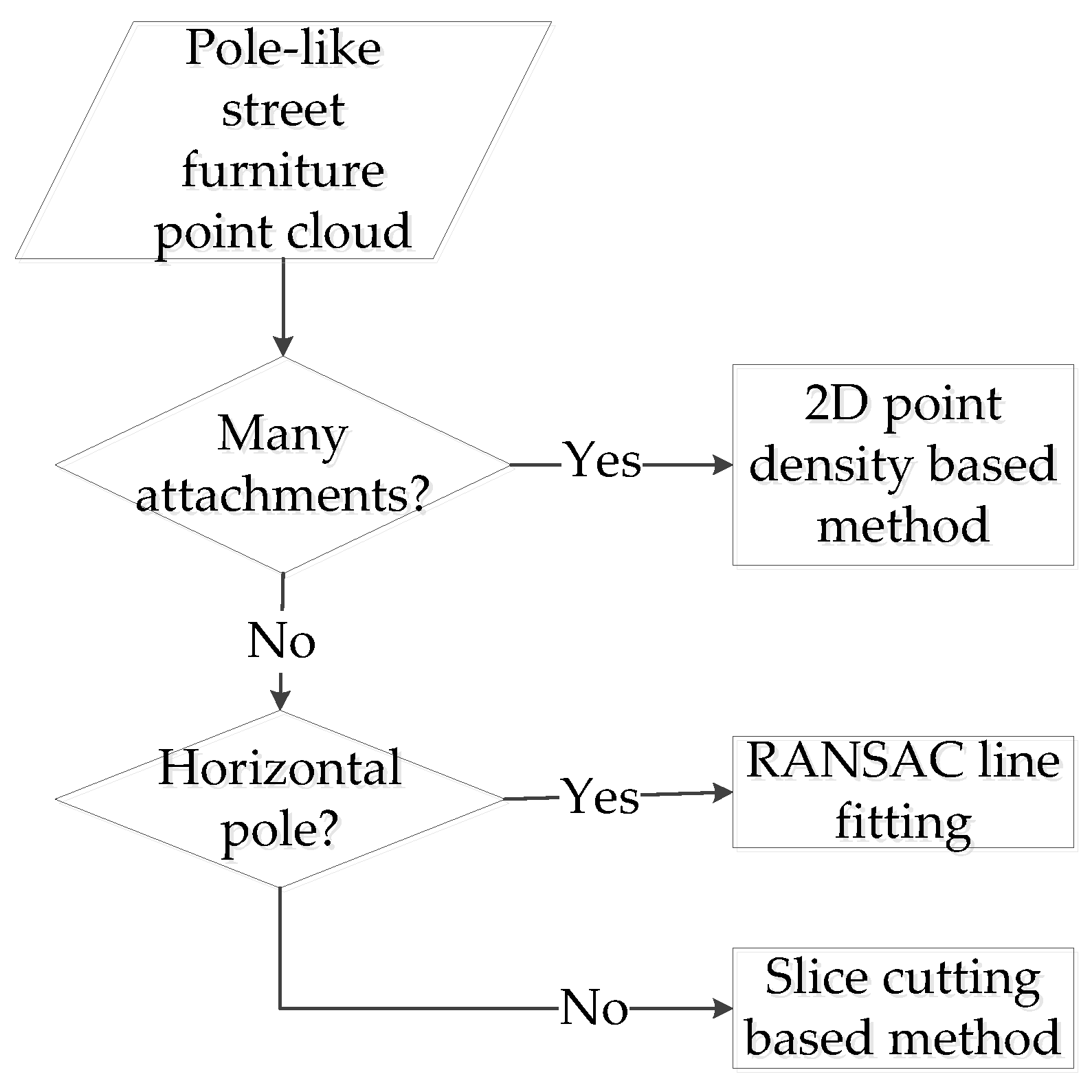
Figure 9.
The pole extraction. (a) Pole extraction using the 2D point density-based method; (b) pole extraction using the RANSAC-based line fitting method; (c) pole-extraction using the slice cutting based method.
Figure 9.
The pole extraction. (a) Pole extraction using the 2D point density-based method; (b) pole extraction using the RANSAC-based line fitting method; (c) pole-extraction using the slice cutting based method.
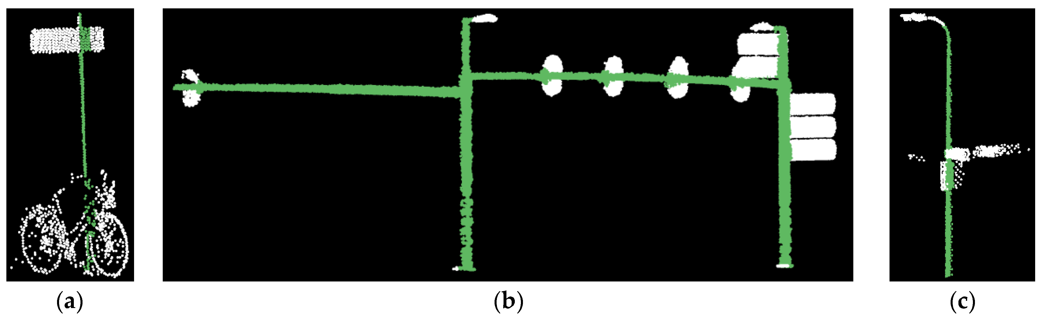
Figure 10.
The extracted center lines of poles. The red lines are the extracted center lines of the pole. (a) The extracted center lines were inclined towards the street side and (b) the optimized center lines.
Figure 10.
The extracted center lines of poles. The red lines are the extracted center lines of the pole. (a) The extracted center lines were inclined towards the street side and (b) the optimized center lines.
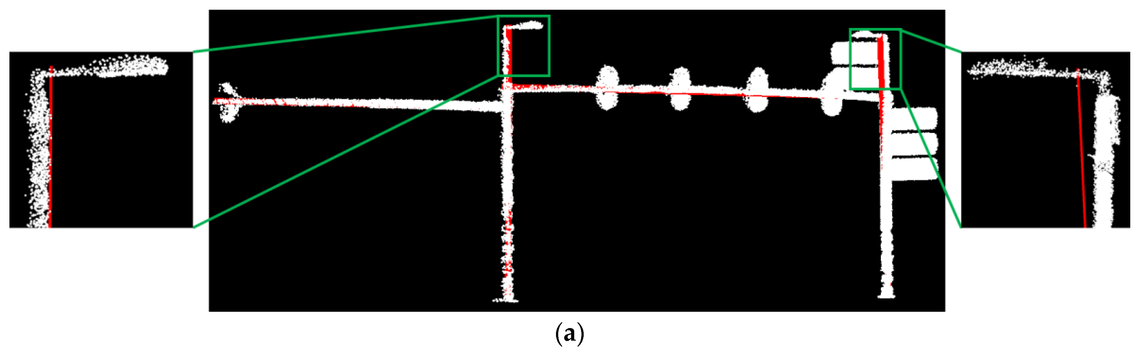

Figure 11.
Examples of the separated components. The separated components after (a) 2D point density-based pole extraction, (b) RANSAC line fitting based pole extraction, (c) and (d) slice cutting based pole-extraction.
Figure 11.
Examples of the separated components. The separated components after (a) 2D point density-based pole extraction, (b) RANSAC line fitting based pole extraction, (c) and (d) slice cutting based pole-extraction.
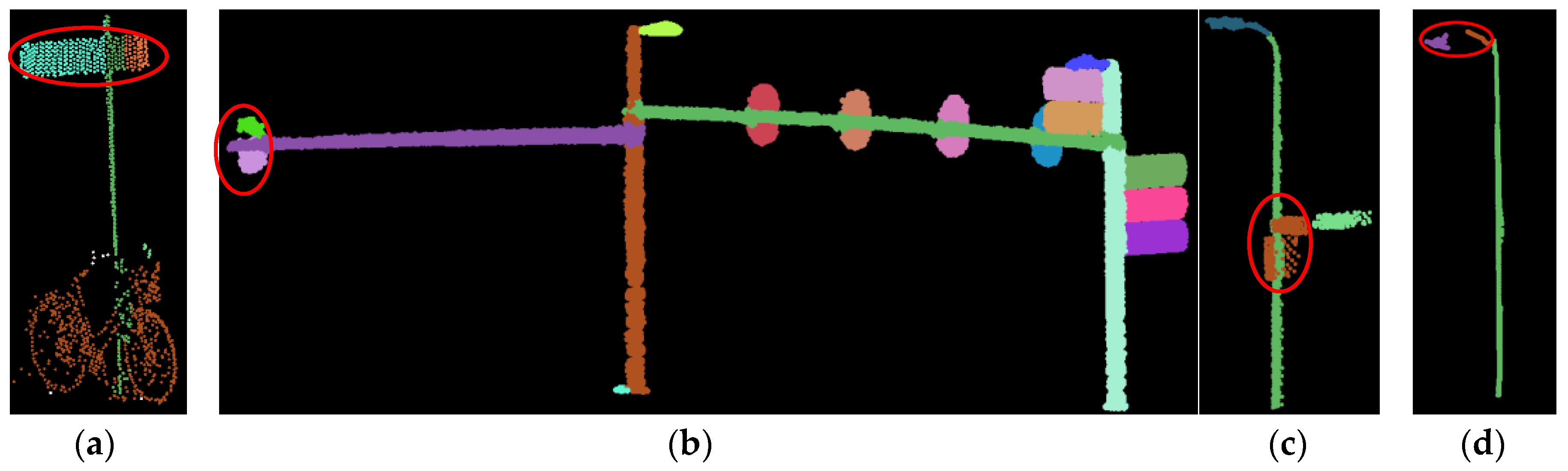
Figure 12.
The left frame is the zoomed in image of the merged component after applying the merging rule.
Figure 12.
The left frame is the zoomed in image of the merged component after applying the merging rule.

Figure 13.
The components connected with vertical poles are split (left) and merged (right) after applying the fitting rules.
Figure 13.
The components connected with vertical poles are split (left) and merged (right) after applying the fitting rules.
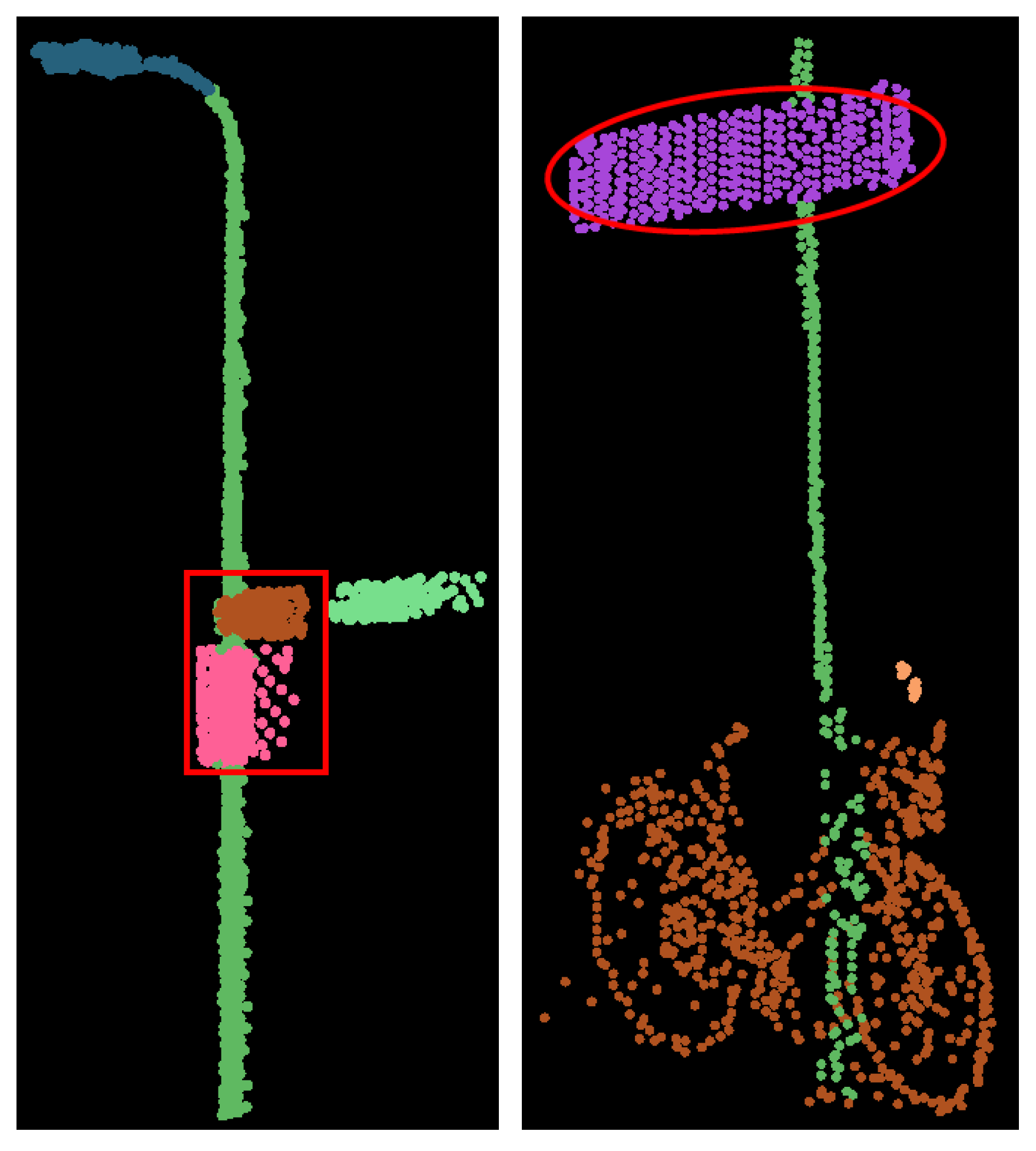
Figure 14.
The detached components merging.

Figure 15.
Examples of the reference data.

Figure 16.
The decomposed components (left) and manually labeled components (right).
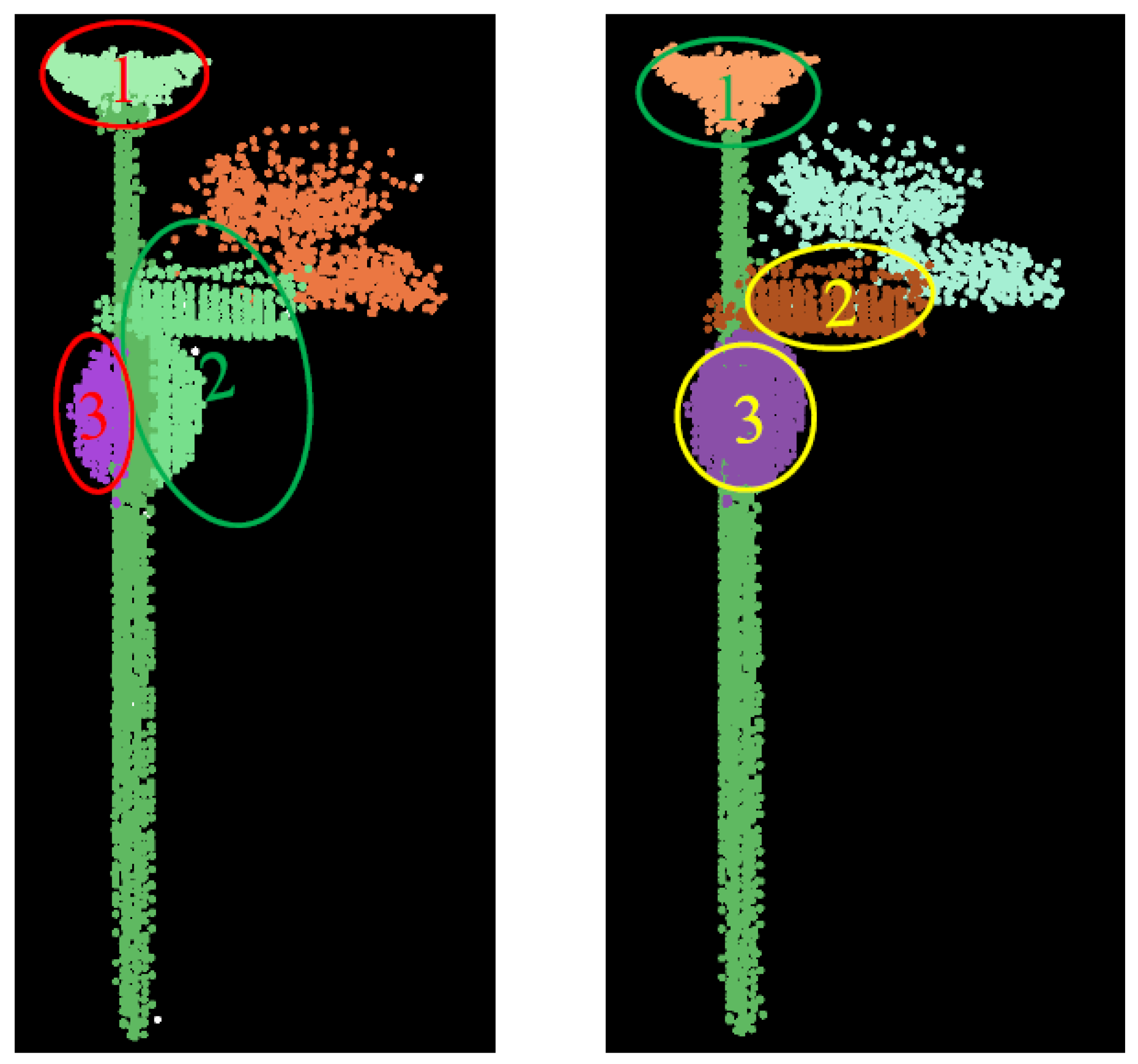
Figure 17.
The pole-like road furniture detection from the Enschede dataset. (a) ground points (white points) and above-ground connected components; (b) detected vegetation (light green), façade (light blue), dynamic objects (light yellow), detected pole-like road furniture (purple), and pole-like furniture connected to vegetation (brown); and (c) the separation of pole-like road furniture connected to trees.

Figure 18.
The occlusion analysis to exclude incorrectly detected pole-like objects inside buildings. (a) The detected pole-like road furniture before occlusion analysis; (b) pole-like road furniture after occlusion analysis.
Figure 18.
The occlusion analysis to exclude incorrectly detected pole-like objects inside buildings. (a) The detected pole-like road furniture before occlusion analysis; (b) pole-like road furniture after occlusion analysis.
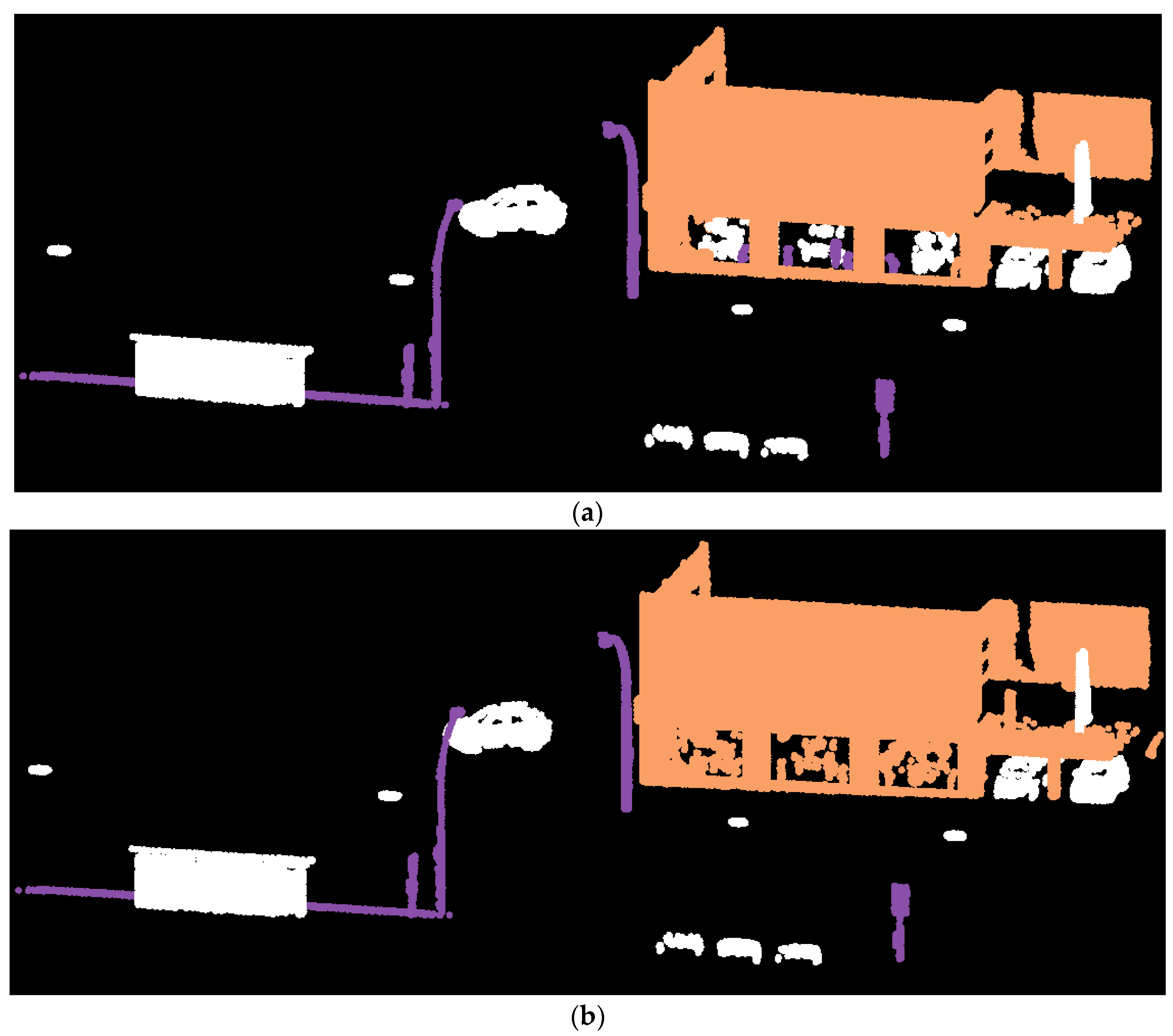
Figure 19.
The pole-like road furniture detection and decomposition from the Enschede dataset. (a) The identified pole-like road furniture (colored by the component number); (b) the decomposition result after applying optimization and rules.
Figure 19.
The pole-like road furniture detection and decomposition from the Enschede dataset. (a) The identified pole-like road furniture (colored by the component number); (b) the decomposition result after applying optimization and rules.

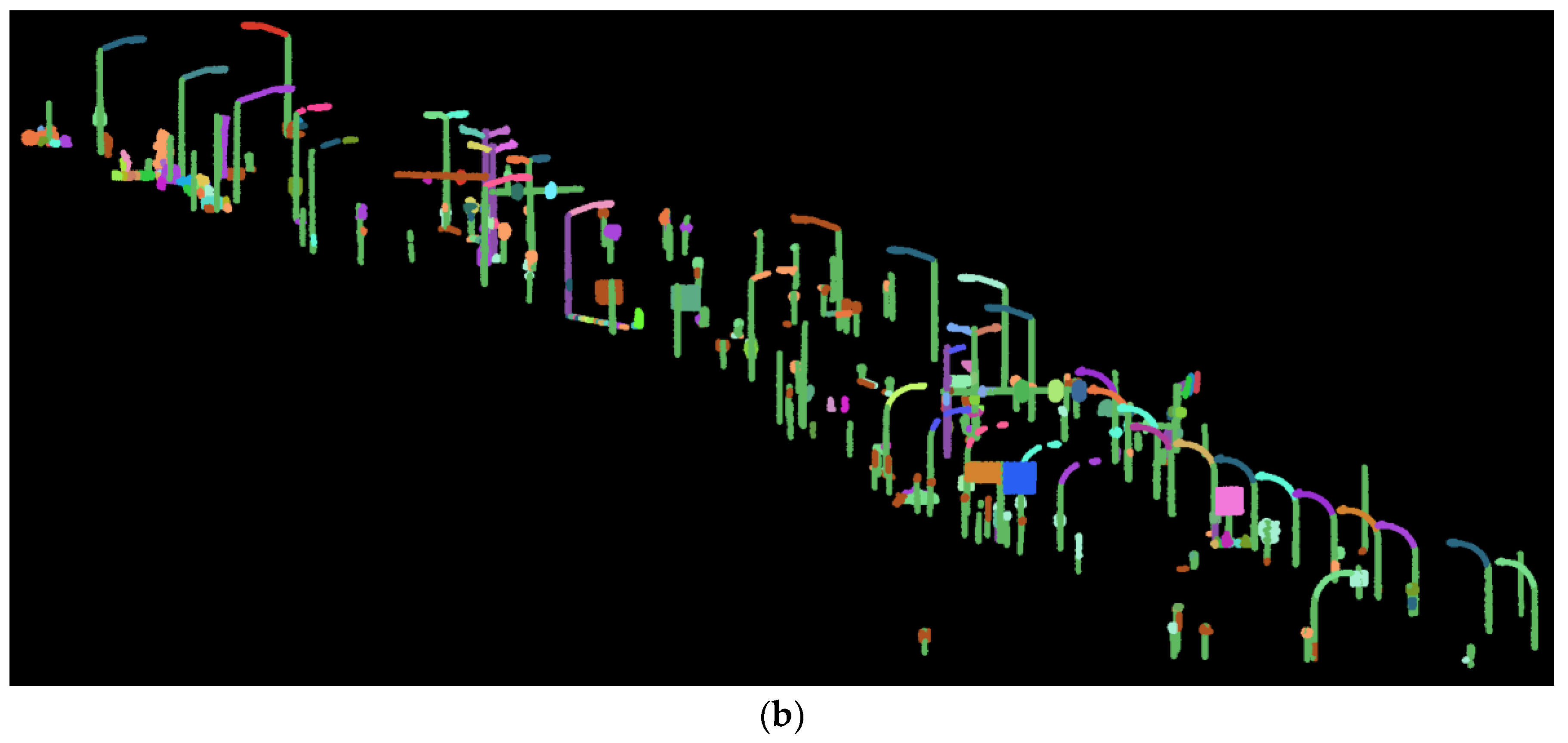
Figure 20.
The pole-like road furniture detection from the Paris dataset. (a) the ground points and above-ground components; (b) the detected façade (light blue) and road furniture (purple). The entities behind façades were incorrectly detected as road furniture in the left green frame; (c) the label of incorrectly detected pole-like objects inside the buildings in the left green frame were redressed after occlusion analysis.

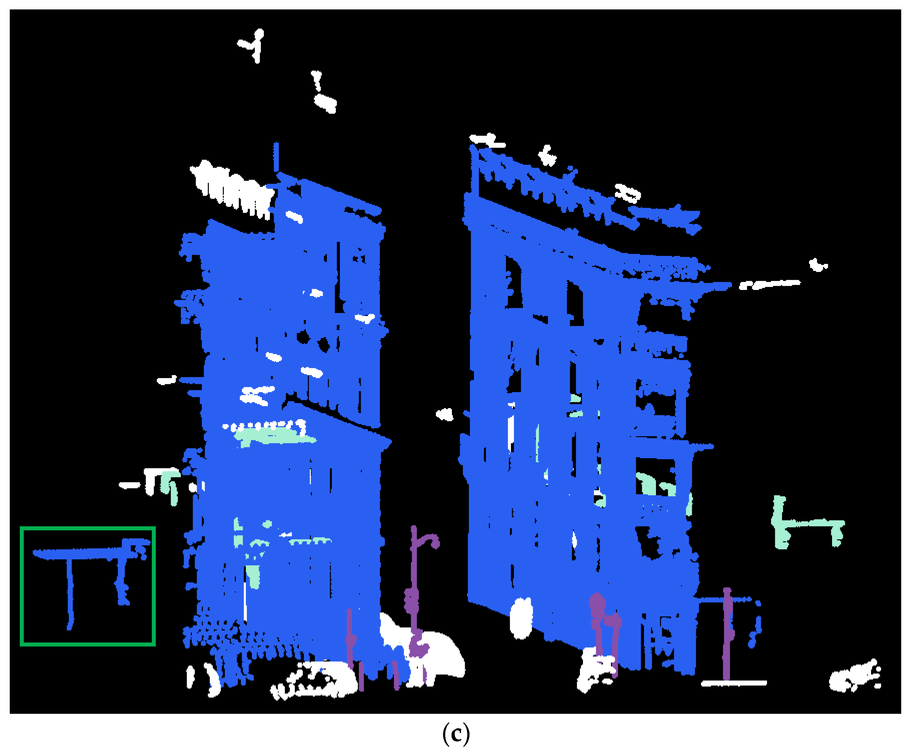
Figure 21.
The pole-like road furniture decomposition from the Paris dataset. (a) The detected pole-like road furniture (colored by component number); (b) the decomposition result after applying optimization and rules.
Figure 21.
The pole-like road furniture decomposition from the Paris dataset. (a) The detected pole-like road furniture (colored by component number); (b) the decomposition result after applying optimization and rules.


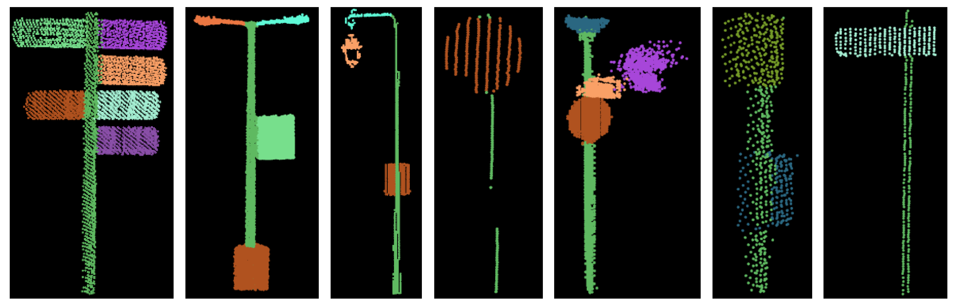
Figure 22.
The correct decomposition results.

Figure 23.
Incorrectly decomposed road furniture. (a) two traffic signs were not separated; (b) one traffic light was decomposed to two fragmented components; (c) the image and (d) the point cloud of two traffic lights which were not separated.
Figure 23.
Incorrectly decomposed road furniture. (a) two traffic signs were not separated; (b) one traffic light was decomposed to two fragmented components; (c) the image and (d) the point cloud of two traffic lights which were not separated.

Table 1.
The accuracy of the road furniture detection in the two test sites.
| Test Site | Enschede, NL |
|---|---|
| Visual interpretation | 151 |
| Correctly detected (before/after the feedback) | 145/143 |
| Total detected (before/after the feedback) | 154/149 |
| Correctness (before/after the feedback) | 94.2%/96.0% |
| Completeness (before/after the feedback) | 96.0%/94.7% |
Table 2.
The accuracy evaluation of the decomposition in the Enschede dataset
| Enschede, NL | Previous Framework | Current Framework | |
|---|---|---|---|
| Point wise | Completeness | 79.5% | 83.2% |
| Correctness | 92.3% | 92.3% | |
| Component wise | Visual inspection | 327 | 327 |
| Correctly decomposed | 236 | 260 | |
| Over-decomposed | 55 | 34 | |
| Under-decomposed | 58 | 54 | |
| Correctness | 72.2% | 79.5% | |
Table 3.
The accuracy evaluation of the decomposition in the Paris dataset.
| Test Site | Paris, FR |
|---|---|
| Visual interpretation | 132 |
| Correctly detected (before/after the feedback) | 126/126 |
| Total detected (before/after the feedback) | 142/138 |
| Correctness (before/after the feedback) | 88.7%/91.3% |
| Completeness (before/after the feedback) | 95.4%/95.4% |
Table 4.
The accuracy evaluation of the decomposition in the Paris dataset.
| Paris, FR | Previous Framework | Current Framework | |
|---|---|---|---|
| Point wise | Completeness | 69.0% | 80.0% |
| Correctness | 90.0% | 92.6% | |
| Component wise | Visual inspection | 125 | 125 |
| Correctly decomposed | 67 | 90 | |
| Over-decomposed | 24 | 12 | |
| Under-decomposed | 45 | 29 | |
| Correctness | 53.6% | 72.0% | |
© 2018 by the authors. Licensee MDPI, Basel, Switzerland. This article is an open access article distributed under the terms and conditions of the Creative Commons Attribution (CC BY) license (http://creativecommons.org/licenses/by/4.0/).
Share and Cite
MDPI and ACS Style
Li, F.; Oude Elberink, S.; Vosselman, G. Pole-Like Road Furniture Detection and Decomposition in Mobile Laser Scanning Data Based on Spatial Relations. Remote Sens. 2018, 10, 531. https://doi.org/10.3390/rs10040531
AMA Style
Li F, Oude Elberink S, Vosselman G. Pole-Like Road Furniture Detection and Decomposition in Mobile Laser Scanning Data Based on Spatial Relations. Remote Sensing. 2018; 10(4):531. https://doi.org/10.3390/rs10040531
Chicago/Turabian StyleLi, Fashuai, Sander Oude Elberink, and George Vosselman. 2018. "Pole-Like Road Furniture Detection and Decomposition in Mobile Laser Scanning Data Based on Spatial Relations" Remote Sensing 10, no. 4: 531. https://doi.org/10.3390/rs10040531
Note that from the first issue of 2016, this journal uses article numbers instead of page numbers. See further details here.