Local Effects of Forests on Temperatures across Europe


1
State Key Laboratory of Remote Sensing Science, Jointly Sponsored by Beijing Normal University and Institute of Remote Sensing and Digital Earth of Chinese Academy of Sciences, Bijian 100875, China
2
Beijing Engineering Research Center for Global Land Remote Sensing Products, Institute of Remote Sensing Science and Engineering, Faculty of Geographical Science, Beijing Normal University, Beijing 100875, China
3
Division of Environment and Sustainability, The Hong Kong University of Science and Technology, Kowloon, Hong Kong, China
*
Author to whom correspondence should be addressed.
Remote Sens. 2018, 10(4), 529; https://doi.org/10.3390/rs10040529
Submission received: 20 December 2017
/
Revised: 22 March 2018
/
Accepted: 27 March 2018
/
Published: 29 March 2018
(This article belongs to the Special Issue Advances in Quantitative Remote Sensing in China – In Memory of Prof. Xiaowen Li)
Abstract
:Forests affect local climate through biophysical processes in terrestrial ecosystems. Due to the spatial and temporal heterogeneity of ecosystems in Europe, climate responses to forests vary considerably with diverse geographic and seasonal patterns. Few studies have used an empirical analysis to examine the effect of forests on temperature and the role of the background climate in Europe. In this study, we aimed to quantitatively determine the effects of forest on temperature in different seasons with MODIS (MODerate-resolution Imaging Spectroradiometer) land surface temperature (LST) data and in situ air temperature measurements. First, we compared the differences in LSTs between forests and nearby open land. Then, we paired 48 flux sites with nearby weather stations to quantify the effects of forests on surface air temperature. Finally, we explored the role of background temperatures on the above forests effects. The results showed that (1) forest in Europe generally increased LST and air temperature in northeastern Europe and decreased LST and air temperature in other areas; (2) the daytime cooling effect was dominate and produced a net cooling effect from forests in the warm season. In the cold season, daytime and nighttime warming effects drove the net effect of forests; (3) the effects of forests on temperatures were mainly negatively correlated with the background temperatures in Europe. Under extreme climate conditions, the cooling effect of forests will be stronger during heatwaves or weaker during cold spring seasons; (4) the background temperature affects the spatiotemporal distribution of differences in albedo and evapotranspiration (forest minus open land), which determines the spatial, seasonal and interannual effects of forests on temperature. The extrapolation of the results could contribute not only to model validation and development but also to appropriate land use policies for future decades under the background of global warming.
1. Introduction
Forests cover more than ~42 million km2 in the Northern Hemisphere (~30% of the land surface), and affects local climate mainly through biophysical processes [1,2,3,4]. The biophysical processes (e.g., albedo, evapotranspiration rate (ET) and surface roughness) all have effects on surface energy fluxes, which causes the effects of forests on local climates to be complicated [5]. Forests usually have a lower albedo than that for grasslands and croplands, especially in winter, when grass or crops are covered by snow. When open land, (i.e. grass or crops), are converted into forests, or even when a deciduous forest transforms into an evergreen forest, the albedo changes, resulting in a change in regional radiative forcing and surface temperature [6]. The surface roughness and ET of forests tend to be higher than those of open land, especially in summer, when forests have a high leaf area index (LAI). In the daytime, forests tend to cool the local temperature with a high latent heat flux. At nighttime, forests may be store heat and increase the local temperature by strengthening the nocturnal temperature inversion [7,8,9]. Therefore, the balance of these different processes determines the net effect of forest on local climate. A comparison of these biophysical processes between forests and open lands can help us determine the effects of forests on local temperatures, a topic which has been analyzed in previous studies [9,10,11,12,13,14].
Depending on the location, biophysical processes in forests may cause the cooling or warming of local temperatures [15]. In tropical regions, the cooling effect of ET, surface roughness and the larger land sink of CO2 from forests dominates the warming effect induced by albedo; therefore, forest surface temperatures tend to be cooler than open land surface temperatures. In contrast, an opposite effect occurs in the boreal zone, where the warming effect is inferior to the cooling effect and is induced by a higher albedo and a land albedo–sea ice feedback mechanism [16]. Many studies have shown that the effects of forests on temperature show a gradient distribution that gradually changes from cooling to warming from the equator to the poles [17,18,19]. Deforestation significantly reduces air temperatures above 45°N in Asia and North America and leads to warming below 35°N [7,19]. Afforestation can obviously increase the land surface temperature (LST) north of 45°N and reduce the LST south of 35°N in the Northern Hemisphere (NH) [14,18,20].
In fact, biophysical processes vary not only with diverse geographic patterns but also with seasonal patterns, which results in different effects of forests on temperature during different seasons [21,22]. Albedo is affected by soil wetness, soil color and snow cover [23,24]. In winter, the difference in albedo between forests and open land is largest because open land tends to be covered with snow. There are also some differences among different forest types at different latitudes. At the high latitudes, the type of forest is mainly needleleaf, which has a ground and forest canopy that are both easily covered with snow. At lower latitudes in Europe, most forests are either mixed or broadleaf forests, where only the canopy is easily covered with snow. This characteristic causes the albedo difference of forest minus open land to vary in space and with the season [21]. The difference in ET is nearly zero because of the small leaf index and radiation limitation [25]. This result implies that the cooling effect, which result from ET and surface roughness, is weaker than the warming effect of albedo in winter. In contrast, in summer, the difference in albedo is smallest, and the difference in ET is largest in summer, which causes the cooling effect resulting that results from ET and surface roughness to be stronger than the warming effect for albedo. The net effects of periodically changed albedo, surface roughness and ET play roles in the seasonal changes of the net effects of forests on the climate at mid- and high- latitudes [20]. This phenomenon is supported by a recent study that found that the effects of deforestation have a south-north gradient from warming to cooling in winter due to snow-cover, which always warms the local temperature in summer in the eastern United States [10].
Moreover, biophysical processes may also change with a variable background climate in different years, enabling the effects of forests change with years [26]. From a cold year to a warm year, the difference in albedo between forests and open land may decrease because of the lower snow depth. The difference in ET may also change, which is related to the local soil moisture. The change in albedo and ET difference between forests and open land may affect the effects of forests, cooling or warming local temperature. Several model studies found that the cooling effect of deforestation decreased with a warmer background [26,27,28]. However, there are also some disagreements within these model results. Winckler et al. [27] and Armstrong et.al [28] found that this decrease would occur globally, while Pitman et al. [26] found that the cooling of deforestation increased in a lower latitude and decreased in a higher latitude. The effect of the background climate on forest effects must be comprehensively evaluated, particularly for the current decade, which is experiencing intense climate warming.
Europe has a temperate marine ecosystem, a Mediterranean ecosystem and a temperate continental climate. There are also many famous mountains in Europe, such as the Alps, the Apennines and the Pyrenees. Considerable heterogeneity of climate and topography has created complex spatial patterns regarding the effect of forest on temperature. In addition, a growing number of extreme climate events, such as heat waves and extreme precipitation, have been observed throughout Europe due to on-going climate change. These various background climates have also created complex spatial and temporal patterns regarding the effects of forests on temperature.
Over the past few decades, most of the known effects of forests on the climate in Europe have been derived from models, while global climate models were not suitable for the local impacts of forest on climate due to their coarse spatial resolutions and uncertainties in the physical processes, parameterization and input data [5,15]. Regional climate models in Europe are often based on comparisons among climate model outputs for different land cover conditions, with the major difference being that forests in one scenario are replaced by open land conditions in another scenario [29]. However, considerable heterogeneity in the climate and topography of Europe has created complex spatial patterns regarding the effects of forests on temperature. A growing number of extreme climate events, such as heat waves and extreme precipitation, have also created complex temporal patterns regarding the effects of forests on temperature [30]. It is not easy for regional climate models to simulate the complex spatial and temporal patterns of forest effects, and some model studies often show contradictory results [31,32].
There are two kinds of observations, that are widely used to explore the effects of forests on temperature: satellite and in-situ data [7,14,17,18,19,20]. Some studies used satellite observations found that afforestation in China cooled daytime temperatures and warmed the nocturnal temperatures [18,20]. Mi Zhang [19] and Lee et al [7] used forest flux site observations to study the effects of deforestation in North America and eastern Asia and found that deforestation warmed temperature at low latitudes and cooled temperatures at high latitudes. However, few studies have used observations to examine the effects of forests on climate in Europe, which has experienced a large increase in forests over the last two decades. Although Li et al. [14,17] used satellite observation to explore the effect of forest globally and found that forests decrease local temperatures in Europe, they focused on spatial patterns and did not consider the effects of background climate on forests during different yeas. Additionally, using two time observations to represent daily averages may also lead to some uncertainties [33]. Further studies should emphasize the effects of forests on the climate in Europe using both kinds of observations to explore the spatiotemporal patterns of forest effects and the effect of the background climate.
In this paper, we used the MODIS (MODerate resolution Imaging Spectroradiometer) land surface temperature (LST), ET, albedo and land cover classification, and FLUXNET site observations from European Fluxes Database Cluster to analyze the effect of forest on temperature in Europe (11°W - 40°E, 35°N - 70°N) and the effect of the background climate. The specific objectives of this study are as follows: (1) to identify the spatiotemporal pattern of forest effects on LST and air temperature and (2) to explore the impact of the background climate, such as extreme climate, on the forest effects to understand how it impacts temperature.
2. Data and Methods
2.1. Data
The MODIS/Aqua (MYD11A2, version 6) products, with temporal and spatial resolutions of 8 days and 1 km, respectively, from 2003 to 2016, were used in our study because the Aqua satellite passes over the region approximately 13:30 and 01:30, which is close to when the daily maximum and minimum temperatures occur. The MODIS LST data are retrieved from clear-sky conditions over each 8-day period with best quality [34]. Based on the quality control documentation, only temperatures with an emissivity error and an LST error less than or equal to 0.02 and 2 K, respectively, were selected for further study.
The MODIS 16-day/1 km albedo product (MCD43B3 version 5) from 2003 to 2016 was used to calculate the difference in surface albedo between forests and open land (Table 1). The product contains black-sky and white-sky albedo, which can be used to calculate the actual (blue-sky) albedo based on the ratio of direct to diffusive shortwave radiation [35]. In our study, we simply used the averages of black-sky and white sky albedo to represent the blue-sky albedo due to the small difference and high correlation between white-sky and black-sky albedo [14]. The albedo quality in our study was controlled by the MCD43B2 data set, and only pixels that were identified as ‘best quality’, ‘good quality’ and ‘mixed quality’ were chosen for further study. The main reason why we did not choose the version 6 data set was because the albedo product in version 6 had only daily data which was nearly 2 terabytes for our study area and was not convenient to process.
The MODIS ET product (MOD16A2 version 5) was used to quantify the changes in ET (Table 1). The ET product is the first regular 1 km land surface ET data set for the 109.03 million km2 of global vegetation land areas at an 8-day interval [36]. The mean absolute bias of this ET product is approximately 0.33–0.39 mm/day compared with the ET in situ observations. The pixels were only identified as ‘good quality’ or ‘other quality’, but further examination identified the ‘clouds NOT present ‘classification, which was selected for further study. The MODIS ET version 5 product produced data until 2014. Here, we used MODIS ET data from 2003 to 2014. Our study area was located from mid- to high-latitudes. In the version 6 data set, there were many interpolated values at high latitudes in spring, autumn and winter, which were not suitable for our research.
Annual 500 m MODIS land cover data (MCD12Q1 version 5) in 2012 with the International Geosphere–Biosphere Programme (IGBP) classification, was used to classify forests and open land. Evergreen needleleaf forests, evergreen broadleaf forests, deciduous needleleaf forests, deciduous broadleaf forests and mixed forests in the IGBP land cover classification were merged into one forest type. Croplands and grasslands were combined into an open land classification.
Forest flux sites from the European Fluxes Database Cluster and meteorological stations from Global Summary of the Day (GSOD) database in Europe were used in this study. The GSOD database was based on data exchanged under the World Meteorological Organization (WMO) World Weather Watch Program according to WMO Resolution 40 (Cg-XII). In accordance with the requirements of the WMO, the surface meteorological stations need to be in open grasslands and far away from cities and water bodies. The effects of forests on surface air temperature could be analyzed by comparing the air temperature differences between forest flux sites and meteorological stations.
2.2. Data Processing
2.2.1. Data Aggregation Strategy
All MODIS data used in this study were re-projected into a 0.01° resolution. Each year, there were 46 LST, 46 ET, and 46 albedo images. The 46 albedo images were derived from the phased production strategy. First, we aggregated the 8-day or 16-day MODIS data into monthly means using 8-day or 16-day composites every month. Second, we aggregated the monthly averages into annual averages only if a pixel had 12 monthly averages. Third, we aggregated the annual averages into multiple-year averages if a pixel had at least one valid annual average. Fourth, the monthly averages for a single year were all aggregated into multiple-year monthly averages. Finally, we acquired multiple-year monthly and annual averages for LST, albedo and ET; in total, there were 14 years of annual averages for LST and albedo for the period 2003–2016, and 11 years of annual averages for ET for the period 2003–2014.
The temperature data from the forest flux sites were on a half-hour time scale. First, we aggregated the half-hour data set onto a daily time scale. Only if valid values for one day comprised more than 90% of all measurements (48) were the maximum (Tmax), minimum (Tmin) and mean temperatures (Tmean) of that day calculated. Second, we aggregated the daily Tmax, Tmin and Tmean into monthly and annual averages when the valid daily values comprised more than 90% of days in the whole year. Third, we aggregated the monthly and annual averages into multiple-year averages of Tmax, Tmin and Tmean for forests. We chose the 90% threshold as a compromise between accuracy and a sufficient number of valid years.
2.2.2. Window Searching Strategy
In our study, we applied a window searching strategy similar to that of Li et al. [14] to determine all of the available sample windows and compare forests and open land over Europe. Here, the sample windows as squares contained 40 × 40 pixels, which were approximately equal to 40 km × 40 km. Any two adjacent windows were overlapped by 15 pixels. If a window individually had more than 10% of the pixels for forests and open land, and the absolute average elevation difference between the forest and open land pixels was less than 100 m, it was a valid window that was used to calculate the mean differences in LST, albedo and ET between forests and open land. Additionally, to explore the effects of background temperature on forests, we calculated the mean LST for all pixels within a window and regarded it as the background temperature of that window. As a result, there were 3363 windows selected (Figure 1).
2.2.3. Paired Sites Strategy
Here, we developed paired sites between the forest flux sites and the meteorological stations based on the following criteria. For a given forest flux site, we found all meteorological stations near the forest site within 1°. Then, we chose the meteorological station that had the smallest latitudinal distance between the paired site and the forest flux sites. Temperatures from the GSOD data were set at the daily time scale. We applied the same strategy as that for the forest flux sites to obtain the multiple-year monthly and annual averages of Tmax, Tmin and Tmean for open land. Only if the number of valid years in the forest and open land data sets were greater than one was the paired sites deemed valid to calculate the mean differences in Tmax, Tmin and Tmean. Finally, a total of 48 paired sites were obtained (Figure 1, Table S1). The average difference in elevation at the paired sites was 15.7 m, and the largest difference was 776 m, which was in Lavarone, Italy (the IT-Lav site). The average linear distance from the paired sites was approximately 34.3 km, and the longest distance was nearly 99.3 km, which was in Leinefelde, Germany (the DE-Lnf site).
2.2.4. Temperature Differences and Elevation Adjustment Strategy
The effects of forests on local land surface temperature or air temperature was expressed as the LST difference (ΔLST) and the T difference (ΔT) between forest and open land within a window and a paired site.
where LSTf and LSTo represent the average LST of forests and open land pixels in a window, respectively, and Tf and To represent the air temperature at a paired site. Positive (negative) values of ΔLST or ΔT represent forests that are warmer (cooler) than open land. The ET difference and the albedo difference between forests and open land were defined similarly.
ΔLST = LSTf − LSTo
ΔT = Tf − To
Even within a window or a paired site, the elevation difference between forest and open land might be large, which results in a systematic bias in ΔLST and ΔT due to the lapse rate. In our study, we applied the elevation adjustment method from Li et al. [14] to eliminate an elevation-induced bias from the original value. Here, we produced the correct term based the elevation difference (ΔELV) and the regression slope (k), which were calculated from the linear regression of ΔLST or ΔT versus ΔELV.
where ΔLSTa and ΔTa represent the adjusted LST and air temperature differences, respectively. Here, k for daytime, nighttime, and daily ΔLST were 8.6 °C/km, 2.3 °C/km and 5.4 °C/km, respectively. The k values for the differences in Tmax, Tmin and Tmean were 7.2 °C/km, 4.6 °C/km, and 5.8 °C/km, respectively.
ΔLSTa = ΔLST − k*ΔELV
ΔTa = ΔT − k*ΔELV
3. Results
3.1. Geographic Patterns in Temperature Difference
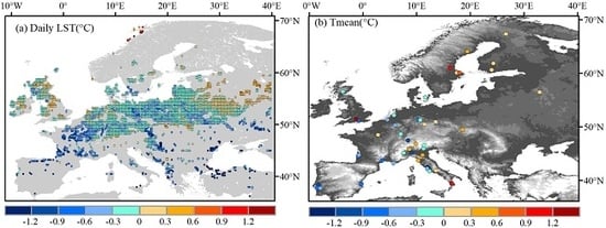
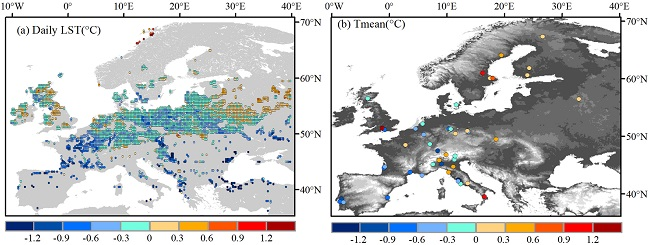
During the daytime, forests have a cooling effect on LST relative to the effect of open land in Europe, except for some areas in England and northern Norway (Figure 2a). The mean annual daytime cooling effect of forests is −1.06 ± 0.03 °C (at the 95% confidence interval and estimated by the t-test; the results hereafter was calculated in the same manner). The cooling effect shows a clear decreasing pattern moving towards higher latitudes and increases slowly with an increase in longitude. Forests cool daytime temperatures within 35°–63°N and warm daytime temperatures north of 66°N. At night, forests tend to have a higher LST than that of open land in Europe, except for a small area in southwest France (Figure 2b). The mean annual nighttime warming effect of forests is 0.58 ± 0.01 °C. The warming effect increases significantly from west to east and decreases slightly towards higher latitudes south of 63°N. Daytime cooling dominates nighttime warming, which results in a daily net cooling in most areas of Europe (Figure 2c). The mean annual daily cooling effect of forests is −0.24 ± 0.01 °C. The cooling effect decreases with an increase in latitudes and longitudes from west to east and transitions into a warming effect over northeastern Europe. In northeastern Europe (north of 55°N and east of 25°E), the mean annual daily warming effect is 0.16 ± 0.03 °C. Similar results are obtained from sampling windows with different sizes or different threshold values of vegetation (figures not shown), suggesting that differences in vegetation type are a major cause of LST differences, which are independent of the vegetation threshold values and sample sizes.
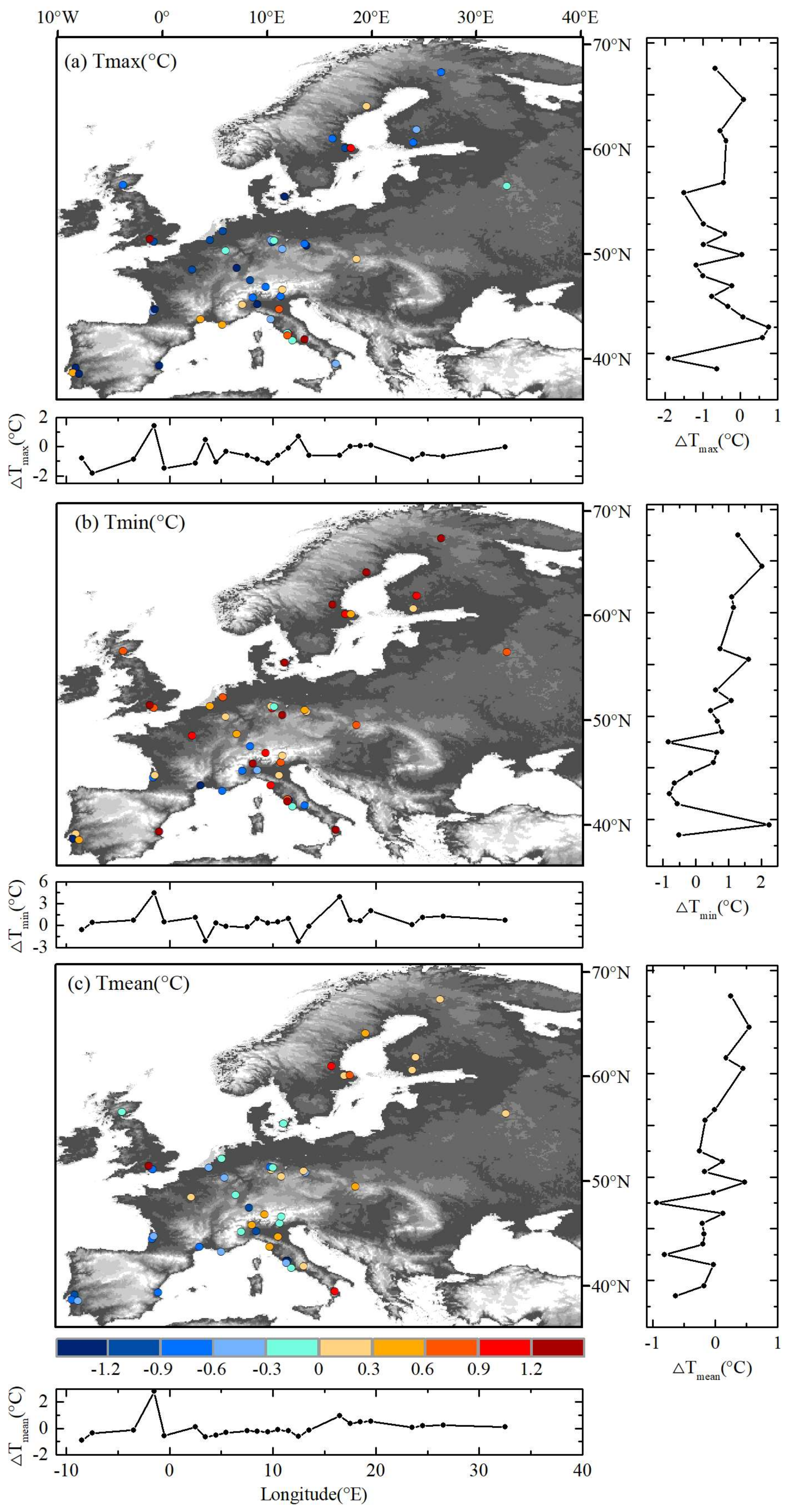
Forests have a similar but slightly different effect on local air temperature. Forests tend to decrease the Tmax and increase the Tmin (Figure 3a,b). However, an adverse phenomenon is found near the Mediterranean area, where forests increase the Tmax and decrease the Tmin. The mean annual Tmax cooling effect and the Tmin warming effect of forests are −0.47 ± 0.28 °C and 0.52 ± 0.44 °C, respectively. The Tmax cooling effect decreases slightly with an increase in longitude, and the Tmin warming effect increases significantly towards higher latitudes, which results in a cooling effect from forests on Tmean in southwestern Europe and a warming effect from forests on Tmean in northwestern Europe (Figure 3c). In southwestern Europe (south of 55°N and west of 15°E), the mean annual cooling effect from forests on Tmean is −0.25 ± 0.23 °C. In northeastern Europe (north of 55°N and east of 15°E), the warming effect from forests on Tmean is 0.36 ± 0.28 °C. Additionally, several paired sites with high elevations have warming effects on Tmean, which is consistent with the results of previous studies [23]. However, some paired sites show an inconsistent phenomenon. For example, one paired site near London and several sites in Italy show a large warming effect on Tmean, while neighboring paired sites have a cooling effect on Tmean, which may result from the background climate and will be discussed in Section 3.3.
3.2. Seasonal Patterns in Temperature Differences
A clear, seasonal variation in the effect of forests on LST can be seen in Europe (Figure 4). Forests cool daytime LSTs during the warm season, and this cooling effect decreases with latitude and increases with longitude (Figure 4a,d). In the cold season, the daytime warming effect dominates all forests, and the effect increases towards high latitudes and with longitude from west to east. The forest nighttime warming effect occurs year-round and increases with longitude (Figure 4b,e). In the warm season, the daytime cooling effect dominates the nighttime warming effect, which results in a net daily cooling effect. The daily cooling effect on LST decreases from low to high latitudes and increases from west to east, which is mainly due to the latitudinal and longitudinal patterns of the daytime cooling effect (Figure 4c,f). In the cold season, forests have a warming effect on LST because of daytime and nighttime warmings. The warming effect increases towards eastern longitudes.
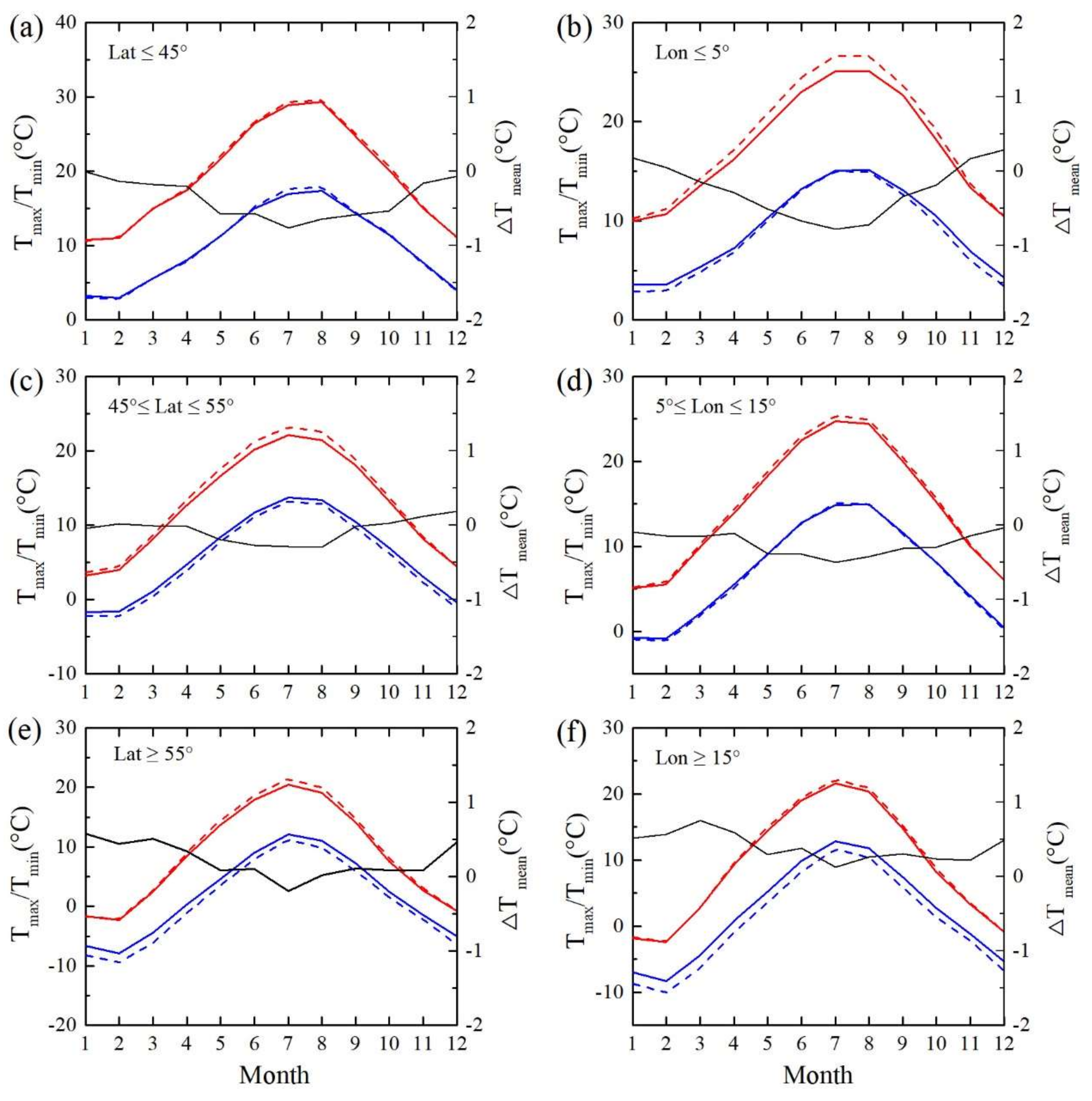
Figure 5 shows the seasonal variations in Tmax and Tmin between forests and open land and their Tmean differences in three different latitudinal and longitudinal zones. Forests tend to have a cooling effect on air temperature during the warm season and a warming effect during the cold season (Figure 5). The mean annual effects of forests on Tmean are −0.37 ± 0.30 °C (number of site pairs: n = 17) below 45°N, −0.07 ± 0.36 °C (n = 21) within 45–55°N and 0.25 ± 0.30 °C (n = 10) north of 55°N. From low latitudes to high latitudes, the cooling effect of forests on Tmax and the warming effect of forests on Tmin both increase. The magnitude of the increase in the cooling effect is weaker than that of the warming effect, which results in a cooling effect from forests on Tmean that decreases with latitude (Figure 5a,c,e). The mean annual effects of forests on Tmean are −0.25 ± 0.65 °C (n = 12) west of 5°E, −0.25 ± 0.20 °C (n = 26) within 5–15°E, and 0.43 ± 0.26 °C (n = 10) east of 15°E. From west to east, the cooling effect of forests on Tmax decreases, and the warming effect of forests on Tmax increases, which results in a cooling effect of forests on Tmean that decreases with an increase in longitude (Figure 5b,d,f).
3.3. Effects of Background Temperatures on the Effects of Forests
The effects of forests on LST and air temperature show both spatial patterns and changes with latitude and longitude, which may be related to background temperatures. In this study, we calculated the average daily LST of all pixels within a window and referred to it as the background LST of a window. For paired sites, we simply regarded the air temperature of a forest site as the background air temperature. Figure 6 shows the relationship between the effects of forests and the background temperature. Forests tend to cool temperatures in warmer locations, such as tropical areas, and warm temperatures in cooler locations, such as arctic and high elevation areas. The same transitional temperature (near 6.5 °C) is found for both LST and air temperature. Forests have a cooling effect when the background temperature is higher than the transitional temperature. In contrast, forests have a warming effect if the background temperature is lower than the transitional temperature.
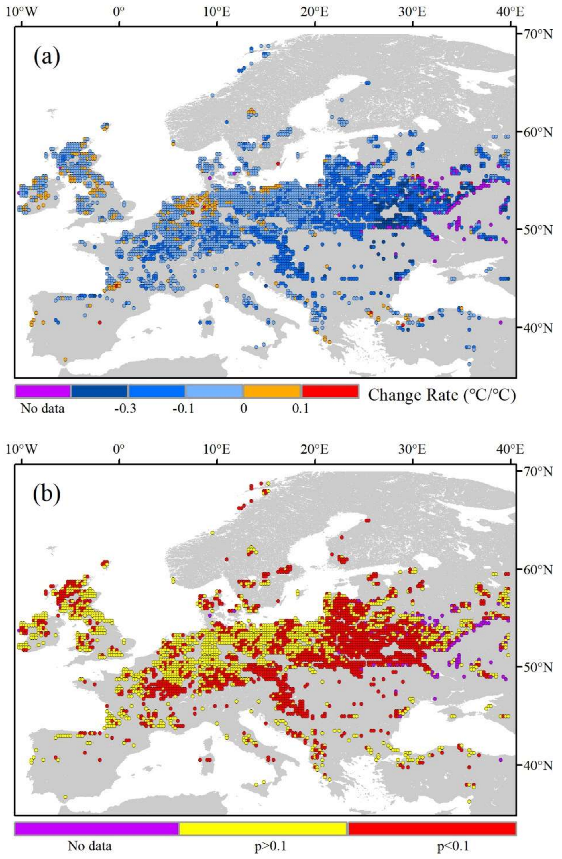
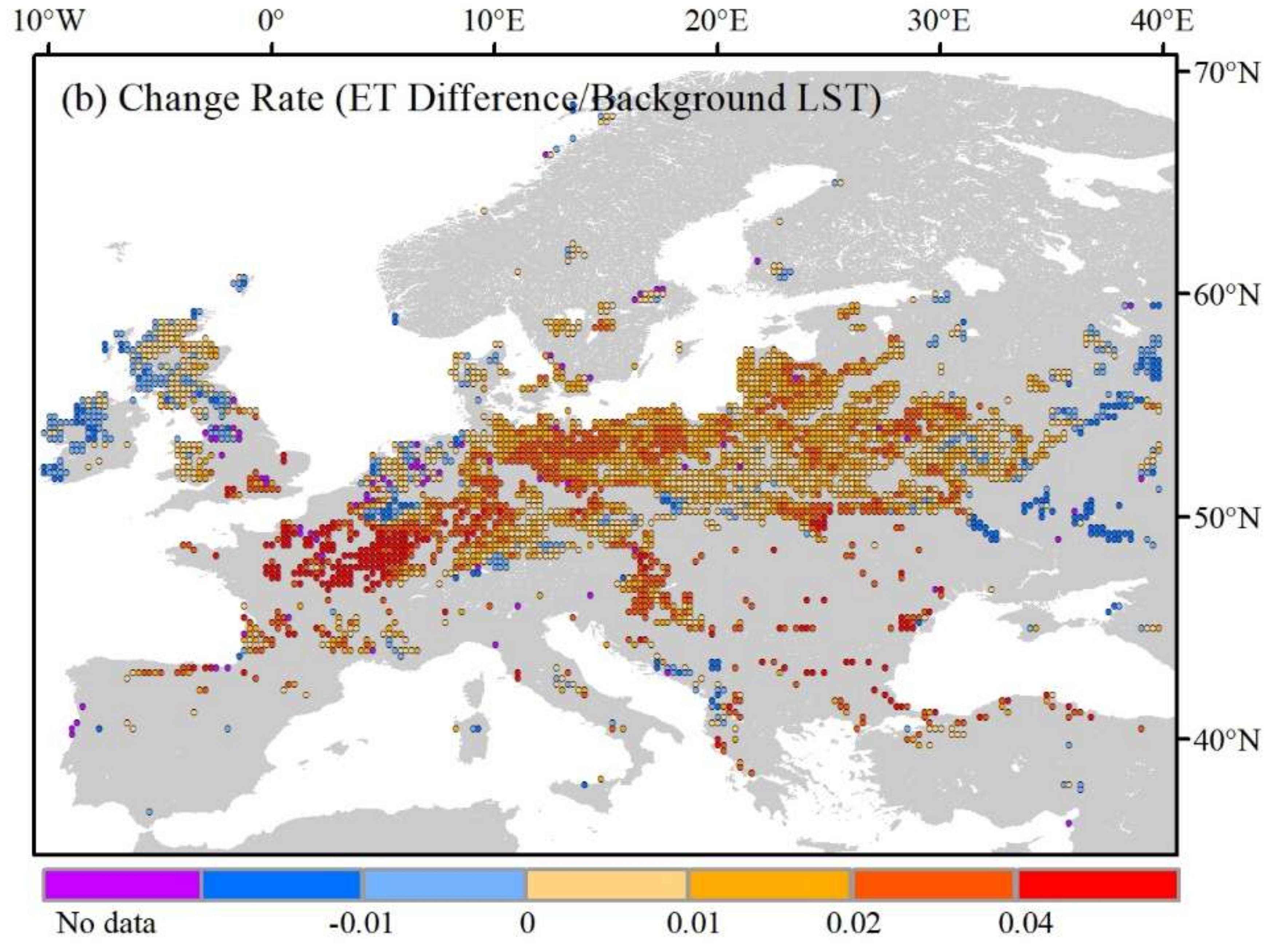
Figure 7 presents the relationship between forest effects and background temperatures for various years. Here, only when the valid years with a window were greater than five years was the relationship between background LST and daily LST differences (forest minus open land) calculated for various years. Since the number of valid years for the paired sites were usually limited, we focused on only the influence of background LSTs on the effects of forests on LST. The daily ΔLST was negatively related to the background LST in most areas of Europe, except for some areas in England and Germany (Figure 7a). This pattern indicated that the cooling effects of forests on LST increased as the background LST increased. Areas with significant changes were mainly located in eastern and southern Europe (Figure 7b).
The effect of background temperature on forest effects is also examined during different seasons (Figure 8). Although the effects of forests are mainly negatively related with background LSTs during the four seasons, there are several differences within the cold seasons (winter and spring) and the warm seasons (summer and autumn). The relationship between background LSTs and the effects of forests is more uniform in cold seasons than that in warm seasons. In spring, the cooling effect of forests tends to increase in eastern Europe and decrease in western Europe as the background LST increases (Figure 8a). In winter, the warming effect of forests decreases in eastern Europe and increases in western Europe as the background LST increases, especially in France (Figure 8d). In summer, the cooling effect of forests decreases in eastern Europe and increases in western Europe as the background LST increases. These relationships are much more complex in autumn, when the cooling effect either increases or decreases as the background LST changes (Figure 8b,c).
3.4. Drivers of Temperature Difference
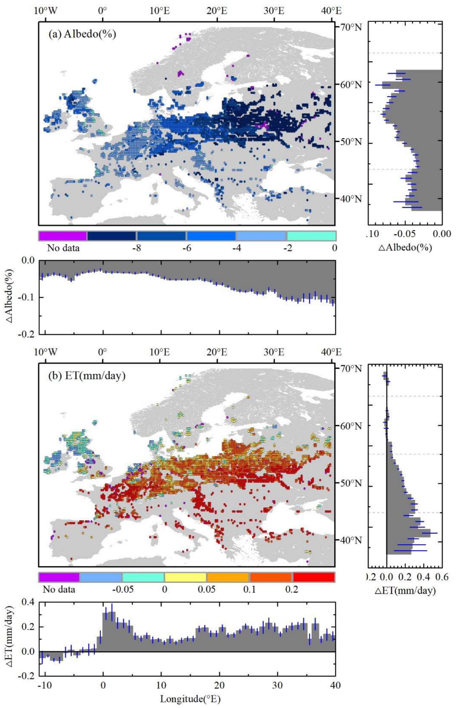
Albedo and ET are identified as key drivers in terms of forest effects. The spatial and seasonal distributions of ΔAlbedo and ΔET are shown in Figure 9 and Figure 10, respectively, which are used to determine if the albedo in forests is lower than that on open lands in all seasons. The difference in albedo increases towards high latitudes and from west to east. Additionally, the difference in albedo is greater in the cold season than that in the warm season. Albedo is affected by soil color and soil wetness. ΔAlbedo is magnified by the presence of snow, as open land can be covered by snow. Snow is more likely to consistently and persistently occur in northern and eastern Europe [37]. Therefore, the ΔAlbedo in northern and eastern Europe is larger than that in western Europe, especially in the winter (Figure 10a,c). Forests have a higher ET than that of open land, especially in the warm season. The difference in ET (forest minus open land) decreases with latitude. For southern Europe, ET is strongly controlled by soil moisture availability, while it is constrained by radiation in northern Europe [25]. Forests can maintain a larger uptake of water because of deeper roots, while open land is more likely to be subjected to water limitations. However, incoming solar radiation over forests is like that of the nearby open land in northern Europe. Thus, the ΔET in southern Europe is greater than that in northern Europe (Figure 9b and Figure 10b).
The spatial and seasonal patterns of differences in albedo and ET (forest minus open land) determine the spatiotemporal differences in LST and T. From south to north, the cooling effect caused by ET differences decreases, while the warming effect caused by albedo differences increases. This results in a cooling effect from forests that decreases with latitude and gradually changes into a warming effect (Figure 2c and Figure 3c). From west to east, the warming effects from albedo increase with longitude; therefore, the cooling effect of forests decreases with longitude in Europe (Figure 2c and Figure 3c). In northeastern Europe, the annual incoming shortwave radiation energy per square meter that is received in the daytime ranges between 1246 and 1835 MJ. The annual mean of ΔAlbedo is −10.39 ± 0.25%. Therefore, forests absorb an extra 129–191 MJ of energy compared with adjacent open lands each year. Moreover, the annual mean ΔET is 0.05 ± 0.01 mm/day in northeastern Europe, which is roughly equivalent to the additional 45 ± 10 MJ of energy that is dissipated from forests compared to that dissipated by open lands each year. The additional energy absorbed by forests via albedo differences is greater than the energy dissipated by forests via ET differences in contrast to open lands, which results in a warming effect from forests in northeastern Europe (Figure 2c and Figure 3c). From the warm season to the cold season, the cooling effect from ET differences decreases, and the warming effect from albedo increases, which results in a net cooling effect from forests in summer and net warming effect from forests in winter (Figure 4 and Figure 5).
The background temperatures during various years may result in different forest effects on local temperature by changing the differences in albedo and ET. Figure 11 shows the relationship between the differences in albedo and ET and background LSTs in Europe. Although some windows have less than five years of valid data, we find that the differences in albedo increase with increasing background LSTs, indicating that the absolute value of the difference in albedo decreases (Figure 11a). The warming effect induced by the difference in albedo decreases when the background temperature increases, especially in eastern Europe, which is significantly affected by snow. The ET difference (forest minus open land) increases with the background LST in most areas of Europe. The cooling effect induced by the difference in ET increases when the background temperature increases. Therefore, the increase in the cooling effect caused by ET and the decrease in the warming effect caused by albedo result in an increase in the net cooling effect of forests on LST (Figure 7a). However, it is noticeable that the difference in ET decreases with an increase in LST in some areas. The change in the cooling effect caused by ET may be complicated under background temperature changes, which results in noise regarding the change in the net effect during warm seasons (Figure 8b,c). In Figure 3c, we observe a paired site that has a strong warming effect from forests near London. This was induced by a heat wave in 2006. In 2006, the annual temperature difference (forest minus open land) was nearly 6 °C, while in normal years, the temperature difference was 1.2 °C. The paired sites in Italy were also strongly affected by the local background temperature. This effect will require further examination in the future.
4. Discussion
In this study, we use satellite observations and in situ measurements to examine the effects of forests on local surface temperatures. Overall, our results show that forests cool surface temperatures in Europe. Our findings agree with those of previous studies to a certain extent. Arora et al. proved that the bio-geophysical component of net temperature responses to 100% afforestation simulations was greater than zero in northeastern Europe and less than zero in other European regions [38]. Montenegro et al. studied the effect of afforestation on biochemical and biophysical processes using satellite data to investigate the effects of afforestation on temperature and proved that afforestation lowered the temperature in areas between 40°S and 60°N [39]. In this paper, an analysis based on measurements demonstrated that forests increase surface temperatures only in northeastern Europe and decrease temperatures in other European areas.
The diurnal asymmetry in temperature results from different energy balance processes, such as solar heating and radiative and dynamic cooling [40]. Daytime temperatures can be modified by incoming solar radiation, land surface properties (e.g., albedo and emissivity), latent and sensible heat fluxes, air mass advection and near-surface atmospheric boundary layer conditions [41]. Given the small size of a single grid cell, incoming solar radiation is likely to be similar in each grid cell. Thus, the amount of absorbed radiation is determined by surface albedo. The consumption of this energy by either latent and sensible heat fluxes or heat storage in soil and biomasses is controlled by vegetation activity and the soil moisture status [36]. In the daytime, due to deeper roots and larger leaf areas, forests have higher efficiencies in dissipating heat into the atmospheric boundary layer through turbulent diffusion than do open lands, which are aerodynamically smoother [42]. Forests absorb more solar energy and dissipate more energy than open land; these two processes determine the daytime ΔLST. Nighttime ET from vegetation is negligible; therefore, nighttime LST is mainly influenced by energy stored during the day and the near-surface atmospheric boundary layer. Lee et al (2011) hypothesized that forests tend to be warmer than open lands at night because forests are usually taller than open land, which enhances turbulence and draws heat from aloft towards the surface [7]. Several similar mechanisms have been proposed for wind farms and orchards, where machines are used to promote turbulence at night to warm the surface temperature [41,43]. Other factors (e.g., soil moisture, air humidity and boundary layer clouds) also help warm surface temperatures at night. The increase in soil moisture for forests tends to increase the surface heat capacity, which results in increases in daytime heat storage and nighttime heating. In addition, due to the higher ET from forests relative to open land, the increases in air humidity and boundary layer clouds increase the downward longwave radiation from the atmosphere and decrease the upward longwave radiation from the surface, which increases surface temperatures at night [9,15,17].
In our study, we found that background temperature was an important factor when determining the effects of forests not only in space but also at the interannual timescale. Forests tend to decrease the local temperature in warmer areas and increase the local temperature in colder areas, which generates a transitional latitude (56°N) and a transitional background temperature (near 6.5 °C) in Europe and causes the cooling effect to switch to a warming effect. Several previous studies that focused on North America and Asia also found a transitional temperature change latitudinally, which was different than that for Europe [7,14,18,19,20]. Latitudinal profiles of the zonal means were derived for air temperatures north of 10°N in North America, Asia, Europe and the Northern Hemisphere. These patterns were calculated via a monthly temperature data set with a spatial resolution of 0.5°, which was obtained from the Climate Research Unit (CRU), version TS3.22 [44,45,46]. We found that the annual mean air temperature (6.5 °C) occurs at 45°N in North America, 45°N in Asia, 56°N in Europe and 46°N in the Northern Hemisphere (Figure 12). Even though a different transitional latitude was observed in Europe than in those studies that observed different continents, the background temperatures were very close at these transitional latitudes.
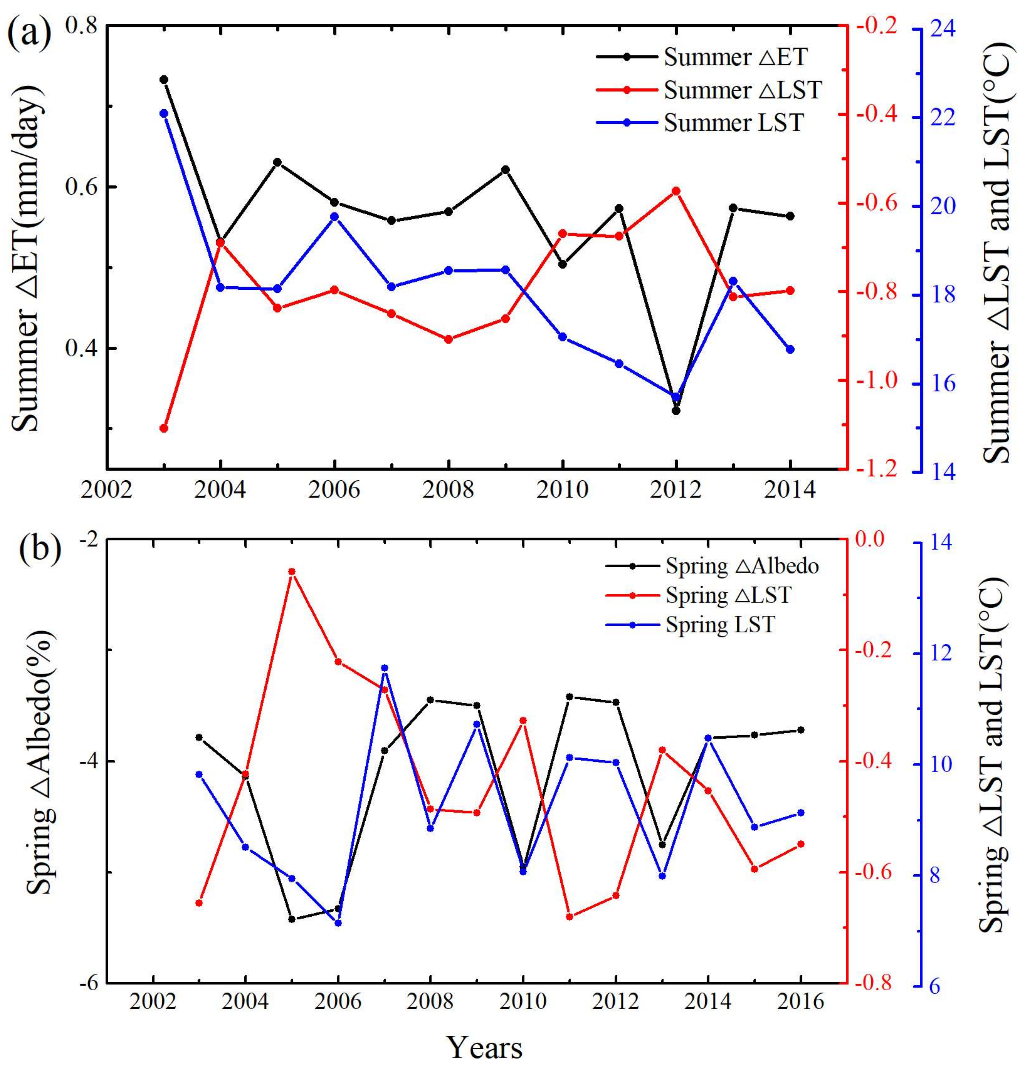
There were record-breaking heatwaves in Europe in 2003 [30,47]. When calculating the average summer ΔLST in central Europe (45°–52°N, 5°–10°E) during the period 2003–2014, we found that the cooling effect of forests in the summer of 2003 was relatively larger than those in other years (Figure 13a), which was consistent with previous findings. For open lands, there was a significantly greater decrease in LAI, which is an important factor influencing ET that amplified the decrease in ET and resulted in a larger ΔET. This phenomenon was most remarkable in central Europe, where the largest number of severe heat waves have occurred. A long, continuous period with temperatures below 0 °C affected large parts of central Europe in 2005/2006, which resulted in a delayed snow melt in the spring of 2006 [37]. We also found that the average spring ΔLST in 2006 was higher than those in other years, which indicated that the cooling effect from forests decreased with colder background temperatures. The main reason for this phenomenon was that the difference in albedo (forest minus open land) became larger when there was a longer snow cover duration in spring, which led to a smaller cooling effect from forests (Figure 13b).
Background temperatures may be a major factor that can influence the effects of forests on temperature by altering biophysical processes, such as the differences in albedo and ET (forest minus open land). Under a warmer climate background, the warming effect caused by albedo is smaller due to reduced snow cover [15,27]. The difference in ET between forests and open lands may decrease in regions with a sufficient amount of soil moisture, but it increases when a region experiences soil moisture depletion [48]. Thus, the change in the cooling effect caused by ET has a greater uncertainty under a warmer background, and it may vary in space as the degree of the background temperature increases. In most areas of Europe, a decrease in the warming effect and an increase in the cooling effect from forest results in an increase in the total forest cooling effect under warmer background temperatures.
In our study, we combined evergreen forests and deciduous forests, which may result in several uncertainties. During the growing season, these two forests are not very different. During the non-growing season, transpiration from evergreen forests may be higher than that from deciduous forests [11]. This means that the cooling effect caused by ET in evergreen forests is greater than that in deciduous forests. However, compared with evergreen forests, deciduous forests are more easily covered with snow, which means that the difference in albedo between evergreen forests and open lands tends to be larger than that between deciduous forests and open lands [30]. The warming effect caused by albedo from evergreen forests is greater than that from deciduous forests. Although there may be different effects between evergreen forests and deciduous forests, the total difference in the effect on local temperature may be small due to the divergent effect (i.e., larger cooling from ET and larger warming from albedo in evergreen forests).
There are several other uncertainties and influential factors in our study. Although MODIS LST has relatively low uncertainties compared with most LST satellite data, there are still some unavoidable uncertainties (i.e., clouds) in the data set [49]. When we study the differences in LST between forests and open lands, uncertainties still exist. In our study, we ignore the measurement height differences between the forest flux sites and the meteorological stations, which may also cause some uncertainties. The height of the temperature measurement in the FLUXNET network varies from 2 to 15 m above the canopy, while the height of measurement at the meteorological stations is 2 m, which may change the annual mean temperature difference by a maximum of 0.008 °C [7]. In addition, we use temporal land cover data instead of long-term unchanged land cover data, which may cause some uncertainties in our results. In addition, numerous factors can affect biophysical processes, which determine the effects of forests on local temperature. Other factors, such as the leaf area index (LAI), root depth, soil moisture, and extreme climate and background temperatures can influence the effects of forests through biophysical processes.
5. Conclusions
Throughout this work, we analyzed the effects of forests on LST and air temperature in Europe using remote sensing data and in situ measurements to reveal the geographic and seasonal patterns of this effect. Additionally, we explored the influence of background temperatures on the spatial and temporal patterns of forest effects on temperature in Europe.
Our results show that (1) forests generally cool the LST and air temperature in Europe, and the cooling effect varies in space and decreases with increases in latitude and longitude, which causes a switch to a warming effect in northeastern Europe; (2) daytime cooling dominates the effect of forests in the warm seasons. In the cold seasons, the daytime and nighttime warming effects drive the effects of forests; (3) background temperature plays a role in the effects of forests on local temperature, and there is a transitional temperature (6.5 °C) in Europe; and (4) the effects of forests are negatively correlated with the background temperature. For example, the cooling effect from forests are larger in heatwaves and smaller in cold springs. Furthermore, (5) background temperatures affect the spatiotemporal patterns of the differences in albedo and ET (forest minus open land), which determines the spatial, seasonal and interannual effects of forests on temperature. This study reveals that other factors (e.g., LAI, root depth, soil moisture and background temperature) may also have an influence on the effects of forests. Further studies should take more biophysical processes into account and combine satellite data, in situ measurements and model results to examine the effects of forests on surface temperature.
Overall, this study provides an empirical analysis to reveal the geographic and seasonal patterns caused by the effects of forests on surface temperatures and the role of background temperature in forest effects in Europe. Understanding the main drivers of climate responses to forests could provide essential information for adaptation strategies, especially under future climate conditions.
Supplementary Materials
The following are available online at https://www.mdpi.com/2072-4292/10/4/529/s1; Table S1: The information on the forest sites.
Acknowledgments
The authors thank Dr. Tao Zhou and Donghai Wu for their helpful comments, which improved this manuscript. This study was supported by the National Key Research and Development Program of China (No. 2016YFA0600103, No. 2016YFB0501404). We are grateful to the members of the FLUXNET community (http://www.fluxdata.org/DataInfo/default.aspx) and, in particular, the European Eddy Fluxes Database Cluster (http://gaia.agraria.unitus.it/home) for acquiring the forest flux data.
Author Contributions
Bijian Tang and Xiang Zhao conceived and designed the experiments. Bijian Tang and Wenqian Zhao processed and analyzed the data. All authors contributed to the design, writing, and discussion.
Conflicts of Interest
The authors declare no conflict of interest.
References
- Bonan, G.B. Forests and climate change: Forcings, feedbacks, and the climate benefits of forests. Science 2008, 320, 1444–1449. [Google Scholar] [CrossRef] [PubMed]
- Forzieri, G.; Alkama, R.; Miralles, D.G.; Cescatti, A. Satellites reveal contrasting responses of regional climate to the widespread greening of Earth. Science 2017, 356, 1180–1184. [Google Scholar] [CrossRef] [PubMed]
- Zeng, Z.; Piao, S.; Li, L.Z.X.; Zhou, L.; Ciais, P.; Wang, T.; Li, Y.; Lian, X.; Wood, E.F.; Friedlingstein, P.; et al. Climate mitigation from vegetation biophysical feedbacks during the past three decades. Nat. Clim. Chang. 2017, 7, 432–436. [Google Scholar] [CrossRef]
- Bright, R.M.; Davin, E.; O’Halloran, T.; Pongratz, J.; Zhao, K.; Cescatti, A. Local temperature response to land cover and management change driven by non-radiative processes. Nat. Clim. Chang. 2017, 7, 296–302. [Google Scholar] [CrossRef]
- Davin, E.L.; de Noblet-Ducoudre, N. Climatic impact of global-scale Deforestation: Radiative versus nonradiative processes. J. Clim. 2010, 23, 97–112. [Google Scholar] [CrossRef]
- Bright, R.M.; Antón-Fernández, C.; Astrup, R.; Cherubini, F.; Kvalevåg, M.; Strømman, A.H. Climate change implications of shifting forest management strategy in a boreal forest ecosystem of Norway. Glob. Chang. Biol. 2014, 20, 607–621. [Google Scholar] [CrossRef] [PubMed]
- Lee, X.; Goulden, M.L.; Hollinger, D.Y.; Barr, A.; Black, T.A.; Bohrer, G.; Bracho, R.; Drake, B.; Goldstein, A.; Gu, L.; et al. Observed increase in local cooling effect of deforestation at higher latitudes. Nature 2011, 479, 384–387. [Google Scholar] [CrossRef] [PubMed]
- Zhao, Q.; Wentz, E.A.; Murray, A.T. Tree shade coverage optimization in an urban residential environment. Build. Environ. 2017, 115, 269–280. [Google Scholar] [CrossRef]
- Schultz, N.M.; Lawrence, P.J.; Lee, X. Global satellite data highlights the diurnal asymmetry of the surface temperature response to deforestation. J. Geophys. Res. Biogeosci. 2017, 122, 903–917. [Google Scholar] [CrossRef]
- Burakowski, E.; Tawfik, A.; Ouimette, A.; Lepine, L.; Novick, K.; Ollinger, S.; Zarzycki, C.; Bonan, G. The role of surface roughness, albedo, and Bowen ratio on ecosystem energy balance in the Eastern United States. Agric. For. Meteorol. 2017, 249, 367–376. [Google Scholar] [CrossRef]
- Juang, J.Y.; Katul, G.; Siqueira, M.; Stoy, P.; Novick, K. Separating the effects of albedo from eco-physiological changes on surface temperature along a successional chronosequence in the southeastern United States. Geophys. Res. Lett. 2007, 34, L21408. [Google Scholar] [CrossRef]
- Luyssaert, S.; Jammet, M.; Stoy, P.C.; Estel, S.; Pongratz, J.; Ceschia, E.; Churkina, G.; Don, A.; Erb, K.; Ferlicoq, M.; et al. Land management and land-cover change have impacts of similar magnitude on surface temperature. Nat. Clim. Chang. 2014, 4, 389–393. [Google Scholar] [CrossRef]
- Rigden, A.J.; Li, D. Attribution of surface temperature anomalies induced by land use and land cover changes. Geophys. Res. Lett. 2017, 44, 6814–6822. [Google Scholar] [CrossRef]
- Li, Y.; Zhao, M.; Motesharrei, S.; Mu, Q.; Kalnay, E.; Li, S. Local cooling and warming effects of forests based on satellite observations. Nat. Commun. 2015, 6, 6603. [Google Scholar] [CrossRef] [PubMed]
- Li, Y.; De Noblet-Ducoudré, N.; Davin, E.L.; Motesharrei, S.; Zeng, N.; Li, S.; Kalnay, E. The role of spatial scale and background climate in the latitudinal temperature response to deforestation. Earth Syst. Dyn. 2016, 7, 167–181. [Google Scholar] [CrossRef]
- Longobardi, P.; Montenegro, A.; Beltrami, H.; Eby, M. Deforestation induced climate change: Effects of spatial scale. PLoS ONE 2016, 11, e0153357. [Google Scholar] [CrossRef] [PubMed]
- Li, Y.; Zhao, M.; Mildrexler, D.J.; Motesharrei, S.; Mu, Q.; Kalnay, E.; Zhao, F.; Li, S.; Wang, K. Potential and Actual impacts of deforestation and afforestation on land surface temperature. J. Geophys. Res. Atmos. 2016, 121, 14372–14386. [Google Scholar] [CrossRef]
- Peng, S.-S.; Piao, S.; Zeng, Z.; Ciais, P.; Zhou, L.; Li, L.Z.X.; Myneni, R.B.; Yin, Y.; Zeng, H. Afforestation in China cools local land surface temperature. Proc. Natl. Acad. Sci. USA 2014, 111, 2915–2919. [Google Scholar] [CrossRef] [PubMed] [Green Version]
- Zhang, M.; Lee, X.; Yu, G.; Han, S.; Wang, H.; Yan, J.; Zhang, Y.; Li, Y.; Ohta, T.; Hirano, T.; et al. Response of surface air temperature to small-scale land clearing across latitudes. Environ. Res. Lett. 2014, 9, 34002. [Google Scholar] [CrossRef]
- Ma, W.; Jia, G.; Zhang, A. Multiple satellite-based analysis reveals complex climate effects of temperate forests and related energy budget. J. Geophys. Res. Atmos. 2017, 122, 3806–3820. [Google Scholar] [CrossRef]
- Wickham, J.; Wade, T.G.; Riitters, K.H. An isoline separating relatively warm from relatively cool wintertime forest surface temperatures for the southeastern United States. Glob. Planet. Chang. 2014, 120, 46–53. [Google Scholar] [CrossRef]
- Wickham, J.D.; Wade, T.G.; Riitters, K.H. Comparison of cropland and forest surface temperatures across the conterminous United States. Agric. For. Meteorol. 2012, 166–167, 137–143. [Google Scholar] [CrossRef]
- Tudoroiu, M.; Eccel, E.; Gioli, B.; Gianelle, D.; Schume, H.; Genesio, L.; Miglietta, F. Negative elevation-dependent warming trend in the Eastern Alps. Environ. Res. Lett. 2016, 11, 44021. [Google Scholar] [CrossRef]
- Zhao, Q.; Myint, S.W.; Wentz, E.A.; Fan, C. Rooftop surface temperature analysis in an Urban residential environment. Remote Sens. 2015, 7, 12135–12159. [Google Scholar] [CrossRef]
- Seneviratne, S.I.; Corti, T.; Davin, E.L.; Hirschi, M.; Jaeger, E.B.; Lehner, I.; Orlowsky, B.; Teuling, A.J. Investigating soil moisture-climate interactions in a changing climate: A review. Earth-Sci. Rev. 2010, 99, 125–161. [Google Scholar] [CrossRef]
- Pitman, A.J.; Avila, F.B.; Abramowitz, G.; Wang, Y.P.; Phipps, S.J.; de Noblet-Ducoudré, N. Importance of background climate in determining impact of land-cover change on regional climate. Nat. Clim. Chang. 2011, 1, 472–475. [Google Scholar] [CrossRef]
- Winckler, J.; Reick, C.H.; Pongratz, J. Why does the locally induced temperature response to land cover change differ across scenarios? Geophys. Res. Lett. 2017, 44, 3833–3840. [Google Scholar] [CrossRef]
- Armstrong, E.; Valdes, P.; House, J.; Singarayer, J. The role of CO2 and dynamic vegetation on the impact of temperate land-use change in the HadCM3 coupled climate model. Earth Interact. 2016, 20. [Google Scholar] [CrossRef]
- Gálos, B.; Hagemann, S.; Hänsler, A.; Kindermann, G.; Rechid, D.; Sieck, K.; Teichmann, C.; Jacob, D. Case study for the assessment of the biogeophysical effects of a potential afforestation in Europe. Carbon Balance Manag. 2013, 8, 3. [Google Scholar] [CrossRef] [PubMed] [Green Version]
- Teuling, A.J.; Seneviratne, S.I.; Stöckli, R.; Reichstein, M.; Moors, E.; Ciais, P.; Luyssaert, S.; van den Hurk, B.; Ammann, C.; Bernhofer, C.; et al. Contrasting response of European forest and grassland energy exchange to heatwaves. Nat. Geosci. 2010, 3, 722–727. [Google Scholar] [CrossRef]
- Deng, X.; Zhao, C.; Yan, H. Systematic modeling of impacts of land use and land cover changes on regional climate: A review. Adv. Meteorol. 2013, 2013. [Google Scholar] [CrossRef]
- Naudts, K.; Chen, Y.; McGrath, M.J.; Ryder, J.; Valade, A.; Otto, J.; Luyssaert, S. Europes forest management did not mitigate climate warming. Science 2016, 351, 597–600. [Google Scholar] [CrossRef] [PubMed]
- Williamson, S.; Hik, D.; Gamon, J.; Kavanaugh, J.L.; Flowers, G.E. Estimating temperature fields from MODIS land surface temperature and air temperature observations in a sub-arctic alpine environment. Remote Sens. 2014, 6. [Google Scholar] [CrossRef]
- Wan, Z. New refinements and validation of the collection-6 MODIS land-surface temperature/emissivity product. Remote Sens. Environ. 2014, 140, 36–45. [Google Scholar] [CrossRef]
- Schaaf, C.B.; Gao, F.; Strahler, A.H.; Lucht, W.; Li, X.; Tsang, T.; Strugnell, N.C.; Zhang, X.; Jin, Y.; Muller, J.P.; et al. First operational BRDF, albedo nadir reflectance products from MODIS. Remote Sens. Environ. 2002, 83, 135–148. [Google Scholar] [CrossRef]
- Mu, Q.; Zhao, M.; Running, S.W. Improvements to a MODIS global terrestrial evapotranspiration algorithm. Remote Sens. Environ. 2011, 115, 1781–1800. [Google Scholar] [CrossRef]
- Dietz, A.J.; Wohner, C.; Kuenzer, C. European snow cover characteristics between 2000 and 2011 derived from improved modis daily snow cover products. Remote Sens. 2012, 4, 2432–2454. [Google Scholar] [CrossRef]
- Arora, V.K.; Montenegro, A. Small temperature benefits provided by realistic afforestation efforts. Nat. Geosci. 2011, 4, 514–518. [Google Scholar] [CrossRef]
- Montenegro, A.; Eby, M.; Mu, Q.; Mulligan, M.; Weaver, A.J.; Wiebe, E.C.; Zhao, M. The net carbon drawdown of small scale afforestation from satellite observations. Glob. Planet. Chang. 2009, 69, 195–204. [Google Scholar] [CrossRef]
- Hain, C.R.; Anderson, M.C. Estimating morning change in land surface temperature from MODIS day/night observations: Applications for surface energy balance modeling. Geophys. Res. Lett. 2017, 44, 9723–9733. [Google Scholar] [CrossRef] [PubMed]
- Zhou, L.; Tian, Y.; Baidya Roy, S.; Thorncroft, C.; Bosart, L.F.; Hu, Y. Impacts of wind farms on land surface temperature. Nat. Clim. Chang. 2012, 2, 539–543. [Google Scholar] [CrossRef]
- Rotenberg, E.; Yakir, D. Distinct patterns of changes in surface energy budget associated with forestation in the semiarid region. Glob. Chang. Biol. 2011, 17, 1536–1548. [Google Scholar] [CrossRef]
- Tang, B.; Wu, D.; Zhao, X.; Zhou, T.; Zhao, W.; Wei, H. The Observed Impacts of Wind Farms on Local Vegetation Growth in Northern China. Remote Sens. 2017, 9, 332. [Google Scholar] [CrossRef]
- Wu, D.; Zhao, X.; Liang, S.; Zhou, T.; Huang, K.; Tang, B.; Zhao, W. Time-lag effects of global vegetation responses to climate change. Glob. Chang. Biol. 2015, 21, 3520–3531. [Google Scholar] [CrossRef] [PubMed]
- Zhao, W.; Zhao, X.; Zhou, T.; Wu, D.; Tang, B.; Wei, H. Climatic factors driving vegetation declines in the 2005 and 2010 Amazon droughts. PLoS ONE 2017, 12. [Google Scholar] [CrossRef] [PubMed]
- Harris, I.; Jones, P.D.; Osborn, T.J.; Lister, D.H. Updated high-resolution grids of monthly climatic observations—The CRU TS3.10 Dataset. Int. J. Climatol. 2014, 34, 623–642. [Google Scholar] [CrossRef] [Green Version]
- Bevan, S.L.; Los, S.O.; North, P.R.J. Response of vegetation to the 2003 European drought was mitigated by height. Biogeosciences 2014, 11, 2897–2908. [Google Scholar] [CrossRef] [Green Version]
- Anderson, R.G.; Canadell, J.G.; Randerson, J.T.; Jackson, R.B.; Hungate, B.A.; Baldocchi, D.D.; Ban-Weiss, G.A.; Bonan, G.B.; Caldeira, K.; Cao, L.; et al. Biophysical considerations in forestry for climate protection. Front. Ecol. Environ. 2011, 9, 174–182. [Google Scholar] [CrossRef]
- Hulley, G.C.; Hughes, C.G.; Hook, S.J. Quantifying uncertainties in land surface temperature and emissivity retrievals from ASTER and MODIS thermal infrared data. J. Geophys. Res. Atmos. 2012, 117. [Google Scholar] [CrossRef]
Figure 1.
The spatial distributions of land cover types, paired sites and selected windows. The green and orange backgrounds refer to areas with forests and open lands, respectively. The paired sites are marked with red triangles. The blue points refer to the selected windows (0.4 × 0.4°), which have areas with more than 10% of forests and open land. The small panels in the below and right show the sample window numbers at each 1° (longitude and latitude) band.
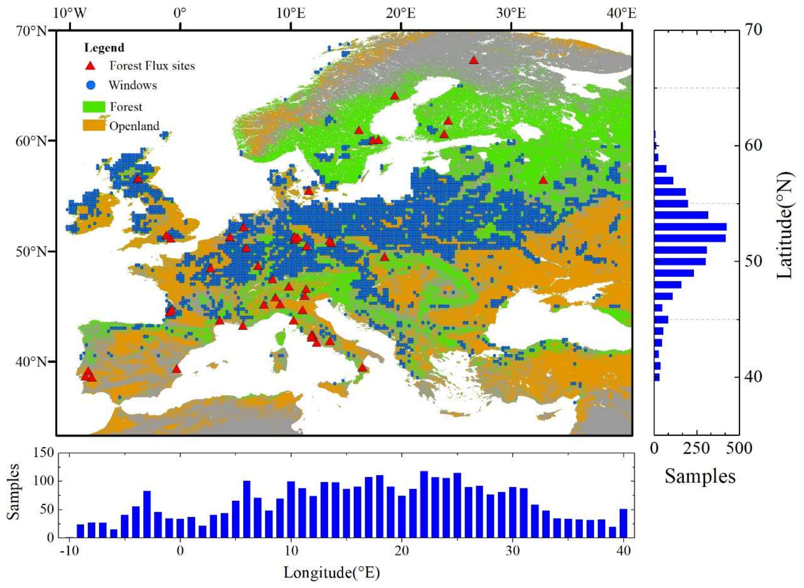
Figure 2.
The spatial distributions of the annual mean (a) daytime, (b) nighttime and (c) daily average ΔLST (forest minus open land) in Europe during the period 2003–2016. The small panels in the below and right of each ΔLST show the longitudinal and latitudinal zonal average of each ΔLST for every 1° bin. The blue lines represent the 95% confidence interval (CI) estimated by the t-test.

Figure 3.
The spatial distributions of the annual mean (a) maximum, (b) minimum and (c) daily average ΔT (forest minus open land) in Europe. The small panels in the below and right show the longitudinal and latitudinal zonal average of each ΔT for every 1° bin. The background color refers to the elevation, which gradually increases from black to white.

Figure 4.
Spatiotemporal patterns of latitudinal variations in (a) daytime, (b) nighttime, (c) daily LST differences (forest minus open land) and longitudinal variations in (d) daytime, (e) nighttime and (f) daily LST differences (forest minus open land) during the period 2003–2016. Grids with cross symbols indicate that the LST differences are significant at the 95% CI by the t-test.
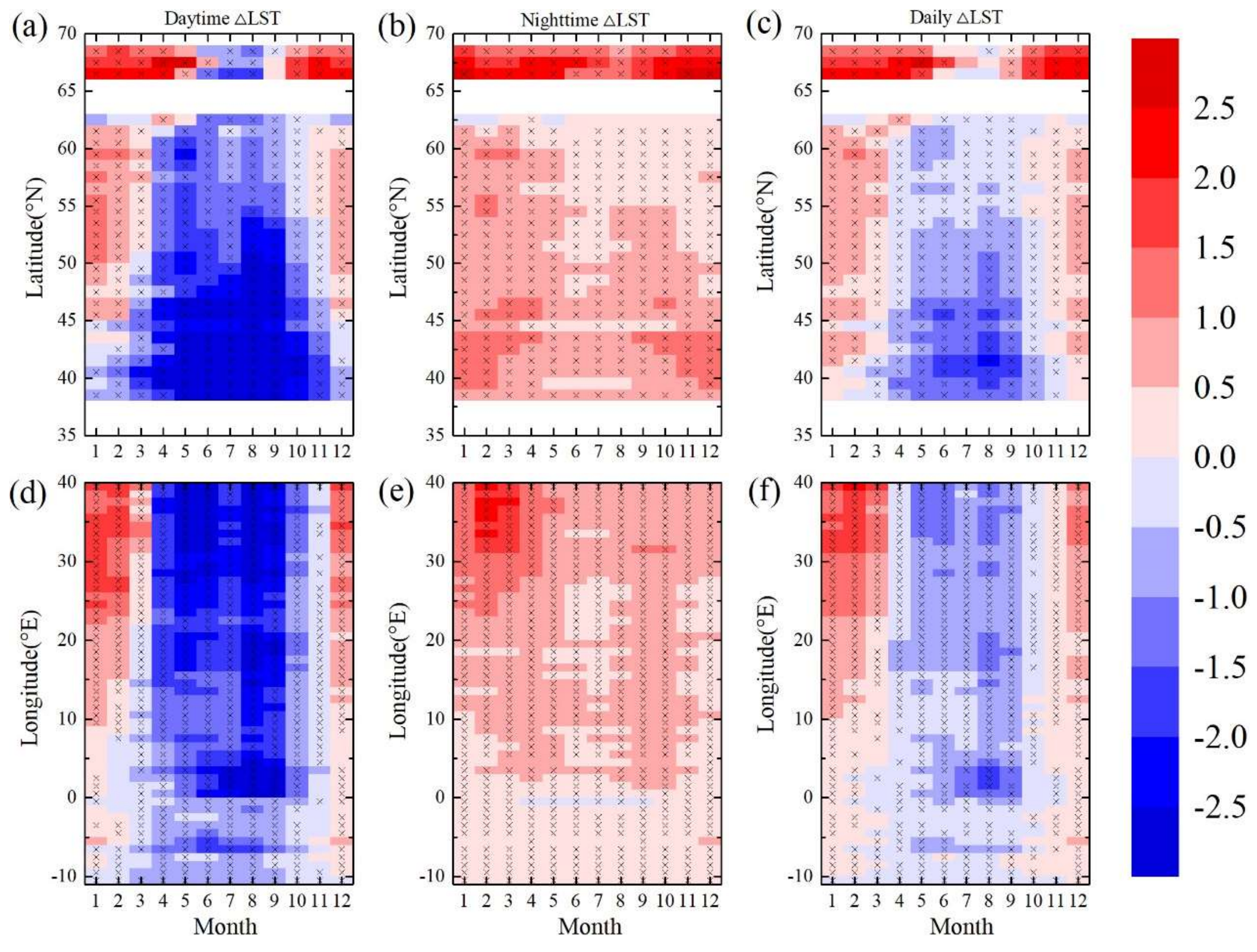
Figure 5.
Comparison of seasonal variations in daily maximum, daily minimum and daily mean temperature differences in three latitudinal (a) south of 45°N, (c) between 45°N and 55°N, (e) north of 55°N, and longitudinal (b) west of 5°E, (d) between 5°E and 15°E, (f) east of 15°E ranges. The red solid and red dashed lines indicate Tmax for forests and open lands, respectively. The blue solid and blue dashed lines indicate Tmin for forests and open lands, respectively. The black solid line indicates the Tmean difference from forests minus open lands.

Figure 6.
The relationships between (a) background LST and daily LST differences (forest minus open land) and (b) background air temperature and daily mean air temperature differences (forest minus open land). The daily LST differences are binned and averaged on 1° background LST intervals (i.e., the LST for all pixels within a window). The daily mean air temperature differences are binned and averaged on 1° grids for background air temperature (i.e., air temperatures of forest sites). The thin black bars represent the 95% confidence interval (CI) by the t-test.
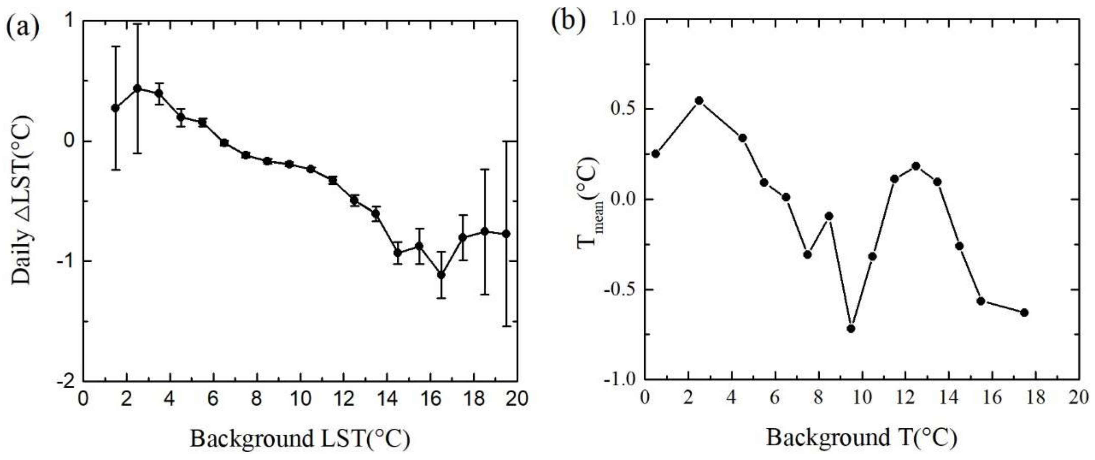
Figure 7.
The relationship between background LST and daily LST differences (forest minus open land) during various years. (a) The rate of change for daily LST differences under different background LSTs. The number 0.1 indicates that the daily LST difference increases by 0.1 °C when the background LST increases by 1 °C. (b) Significance of the relationship between background LST and daily LST differences.

Figure 8.
The relationship between background LST and daily LST differences (forest minus open land) in (a) spring, (b) summer, (c) autumn, and (d) winter during various years. Spring, summer, autumn and winter are defined by March and May, June and August, September and November, and December and February, respectively. The significance map of the four seasons is similar to Figure 7b and is not shown here.
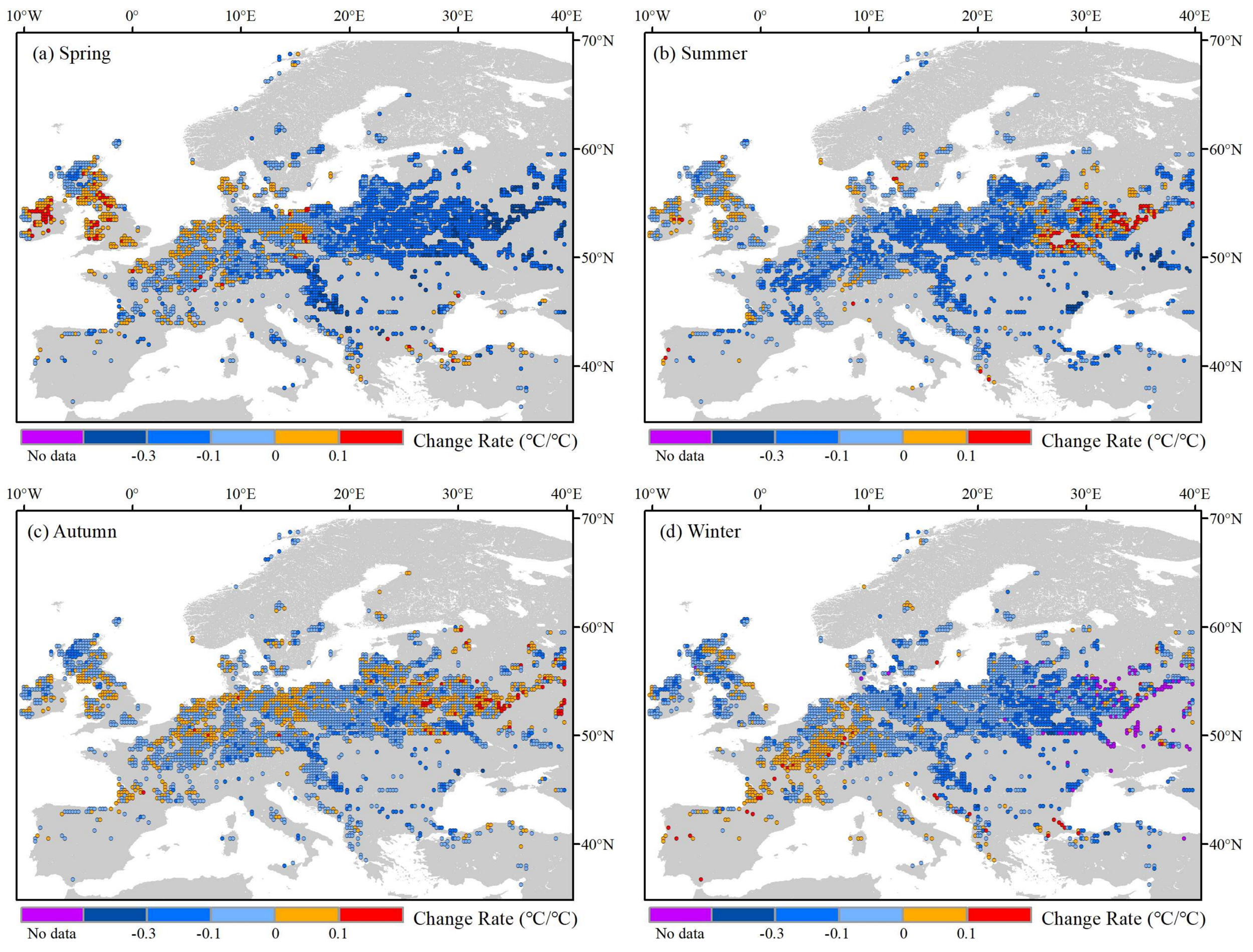
Figure 9.
The spatial distributions of annual mean (a) albedo (%) and (b) ET differences (forest minus open land) in Europe. The periods used to analyze albedo and ET differences are 2003–2016 and 2003–2014, respectively. The below and right small panels for each difference show the longitudinal and latitudinal zonal averages for every 1° bin. The blue lines represent the 95% confidence interval (CI) estimated by the t-test.

Figure 10.
Spatiotemporal patterns of (a) latitudinal and (c) longitudinal variations in albedo (%) differences (forest minus open land) during the period 2003–2016 and (b) latitudinal and (d) longitudinal variations in ET differences (forest minus open land) during the period 2003–2014. Grids with cross symbols indicate differences that are significant at the 95% CI by the t-test.
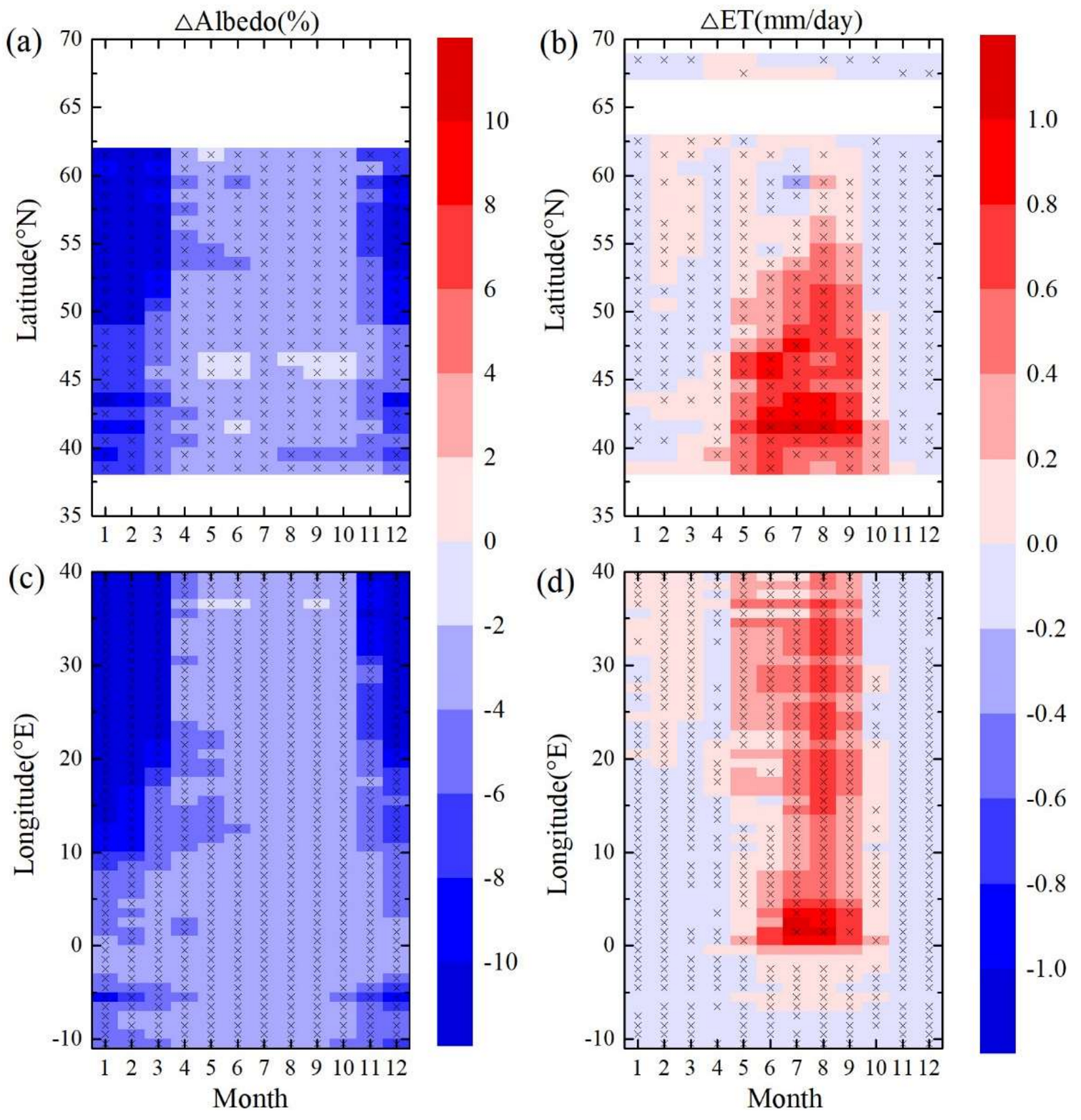
Figure 11.
The relationship between the annual mean background LST and the annual mean (a) albedo (%) differences (forest minus open land) and (b) ET differences (forest minus open land) during various years. The number 0.1 in (a,b) indicates that the albedo and ET differences increase by 0.1% and 0.1 mm/day, respectively, when the background LST increases by 1 °C. Only when the valid year of a window was greater than five years was the relationship calculated.
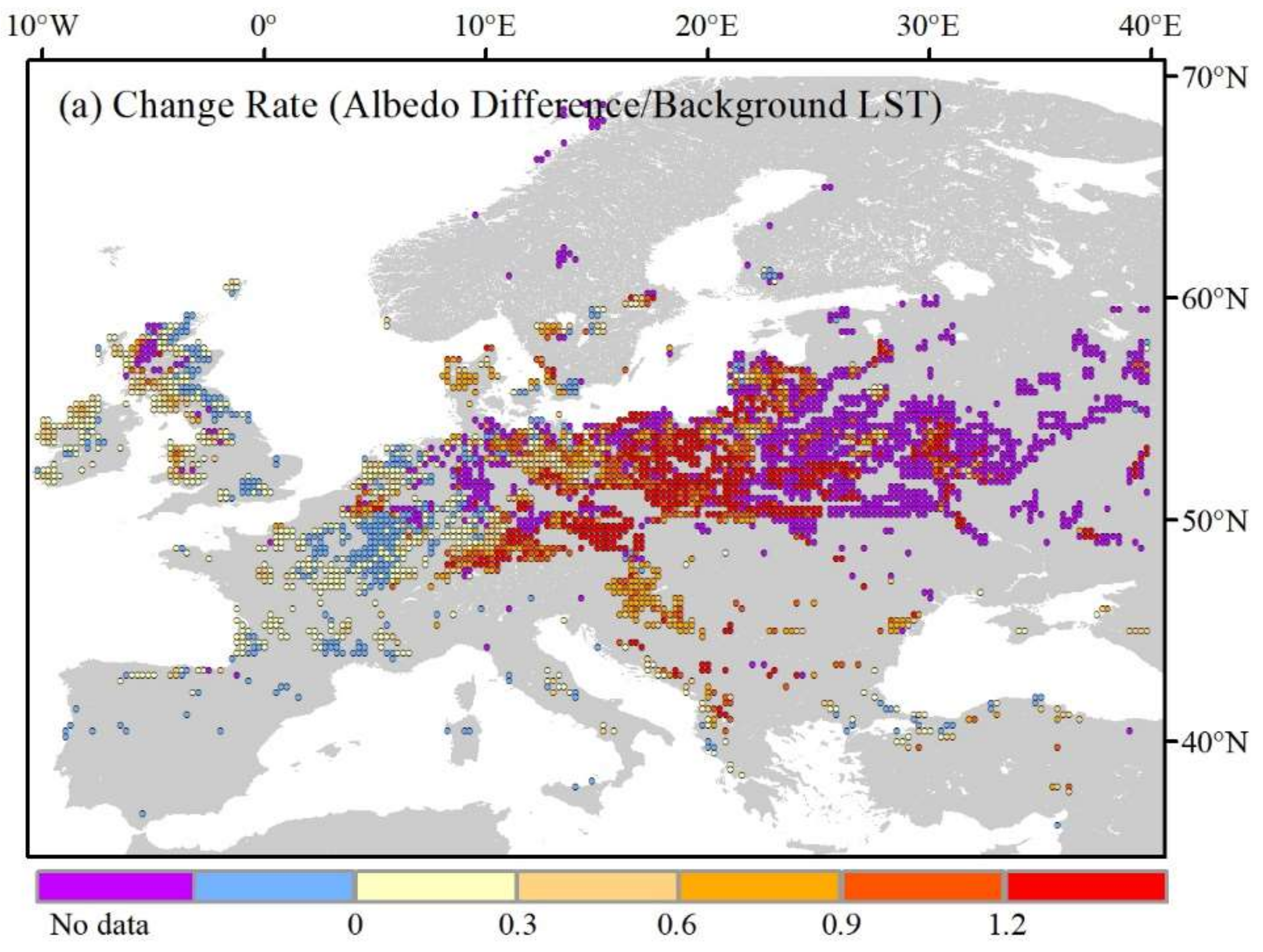

Figure 12.
Annual mean air temperatures at different latitudes in the Northern Hemisphere (north of 10°N) during the period 2003–2016, where NA represents North America, EU represents Europe, AS represents Asia and NH represents the Northern Hemisphere. The dotted line represents 6.5 °C.
Figure 12.
Annual mean air temperatures at different latitudes in the Northern Hemisphere (north of 10°N) during the period 2003–2016, where NA represents North America, EU represents Europe, AS represents Asia and NH represents the Northern Hemisphere. The dotted line represents 6.5 °C.
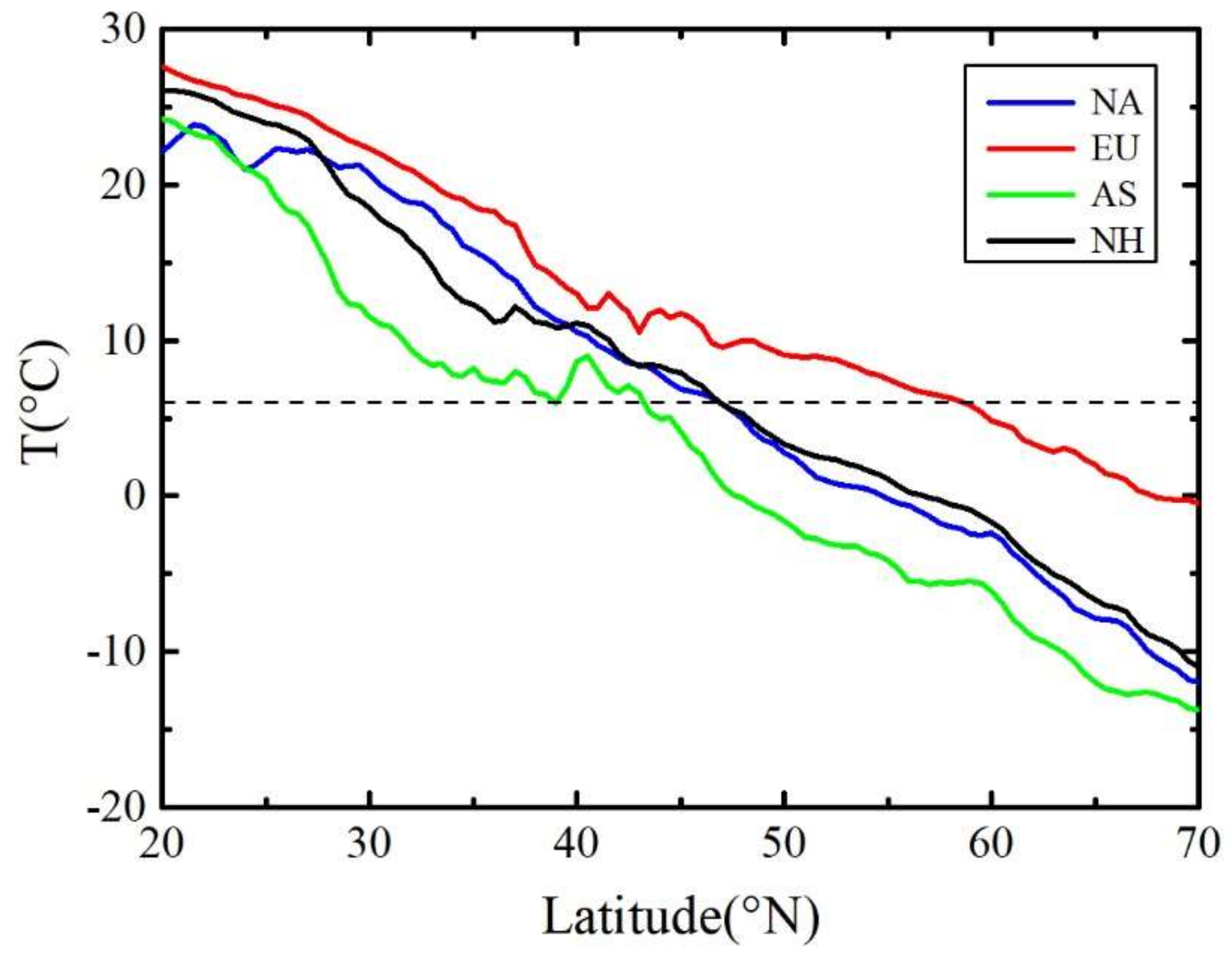
Figure 13.
Interannual variability of (a) the seasonal mean LST in summer, the difference in ET (forest minus open land) in summer, and background LST in summer and (b) the seasonal mean LST in spring, the difference in albedo (forest minus open land) in spring, and the background LST in spring.
Figure 13.
Interannual variability of (a) the seasonal mean LST in summer, the difference in ET (forest minus open land) in summer, and background LST in summer and (b) the seasonal mean LST in spring, the difference in albedo (forest minus open land) in spring, and the background LST in spring.


Table 1.
List of data products used
| Produce Name | Product Type | Resolution | Period Considered |
|---|---|---|---|
| MYD11A2 (V6) | LST | 1 km | 2003–2016 |
| MCD43B3 (V5) | Albedo | 1 km | 2003–2016 |
| MOD16A2 (V5) | ET | 1 km | 2003–2014 |
| MCD12Q1 (V5) | Land cover type | 500 m | 2012 |
| Forest flux sites | Air temperature | Valid year from 1996–2016 |
© 2018 by the authors. Licensee MDPI, Basel, Switzerland. This article is an open access article distributed under the terms and conditions of the Creative Commons Attribution (CC BY) license (http://creativecommons.org/licenses/by/4.0/).
Share and Cite
MDPI and ACS Style
Tang, B.; Zhao, X.; Zhao, W. Local Effects of Forests on Temperatures across Europe. Remote Sens. 2018, 10, 529. https://doi.org/10.3390/rs10040529
AMA Style
Tang B, Zhao X, Zhao W. Local Effects of Forests on Temperatures across Europe. Remote Sensing. 2018; 10(4):529. https://doi.org/10.3390/rs10040529
Chicago/Turabian StyleTang, Bijian, Xiang Zhao, and Wenqian Zhao. 2018. "Local Effects of Forests on Temperatures across Europe" Remote Sensing 10, no. 4: 529. https://doi.org/10.3390/rs10040529
Note that from the first issue of 2016, this journal uses article numbers instead of page numbers. See further details here.