Wavelet-Based Rust Spectral Feature Set (WRSFs): A Novel Spectral Feature Set Based on Continuous Wavelet Transformation for Tracking Progressive Host–Pathogen Interaction of Yellow Rust on Wheat

Abstract

Understanding the progression of host–pathogen interaction through time by hyperspectral features is vital for tracking yellow rust (Puccinia striiformis) development, one of the major diseases of wheat. However, well-designed features are still open issues that impact the performance of relevant models to nondestructively detect pathological progress of wheat rust. The aim of this paper is (1) to propose a novel wavelet-based rust spectral feature set (WRSFs) to uncover wheat rust-related processes; and (2) to evaluate the performance and robustness of the proposed WRSFs and models for retrieving the progression of host–pathogen interaction and tracking rust development. A hyperspectral dataset was collected by analytical spectral devices (ASD) spectroradiometer and Headwall spectrograph, along with corresponding physiological measurements of chlorophyll index (CHL), nitrogen balance index (NBI), anthocyanin index (ANTH), and percentile dry matter (PDM) from the 7th to 41st day after inoculation (dai) under controlled conditions. The resultant findings suggest that the progression of yellow rust on wheat is better characterized by the proposed WRSFs (R² > 0.7). The WRSFs-based PLSR model provides insight into specific leaf biophysical variations in the rust pathological progress. To evaluate the efficiency of the proposed WRSFs on yellow rust discrimination during different infestation stages, the identified WRSFs and vegetation indices (VIs) were fed into linear discriminant analysis (LDA) and support vector machine (SVM) classification frames. The WRSFs in conjunction with a SVM classifier can obtain better performance than that of LDA method and the VIs-based models. Overall, synthesizing the biophysical analysis, retrieving accuracy, and classification performance, we recommend the proposed WRSFs for monitoring the progression of the host–pathogen interaction of yellow rust on wheat cross various hyperspectral sensors.

1. Introduction

Yellow rust (Puccinia striiformis) is one of the most severe epidemic diseases for winter wheat in China, affecting more than 6.7 million ha during 2000–2016 (http://cb.natesc.gov.cn/sites/cb/). Under prolonged stress, crop growth and productivity are impaired [1]. Due to the high costs of chemical control, a real-time nondestructive detection of the pathological progression of rust on leaves is vital for effective management using precision agriculture. Currently, hyperspectral analyses are the main approach for detecting foliar biophysical variations, and provide the basis for tracking rust development in hyperspectral language [2].

The interaction of electromagnetic radiation with plant leaves is governed by their biophysical constituents and response to infestations [3,4,5]. Numerous researches have been undertaken in order to understand these host–pathogen interactions from the hyperspectral perspective [3,6], Most of them attempted to link vegetation indices (VIs), which employ algebraic combination on specific spectral bands with specific foliar constituent [7,8]. For instance, Mahlein, et al. [9] analyzed the hyperspectral signatures of cercospora leaf spot, sugar beet rust and powdery mildew on sugar beet plants, and developed specific vegetation indices to detect and identify various diseases with an overall accuracy of 88.3%. Shi, et al. [10] tested a total of 18 typical spectral features for the classification of yellow rust, powdery mildew, and aphid on wheat. The results showed the potential of VIs-based kernel discriminant analysis (KDA) for detecting various diseases under complicated farmland circumstances.

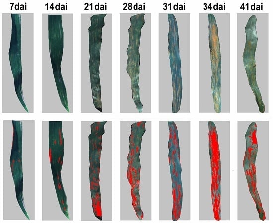
Pathologically, the development of yellow rust comprises five spore stages, uredospores, appressorium, basidiospores, spermatia, and aeciospores. The foliar biophysical variations are critical indicators for tracking the progression of host–pathogen interactions through the different stages. In the initial two stages, uredospores and appressorium develop on the upper side of leaves with random scatter distribution of pustules that are invisible to the naked eye [11]. Subsequently, basidiospores, spermatia and aeciospores grow hyphae and haustorium inside the cellular tissue of leaves, and induce a series of biophysical lesions [12]. Currently, the majority of studies on agricultural diseases monitoring, using earth observation, have focused on a given infestation stage, usually late in the progression of the disease [6,13,14,15,16,17]. Although focusing on late stages of the infestations might maximize the discriminant power of the methods, the outcomes will be less relevant for crop protection as the damage will be detected too late for any efficient actions. Thus, further effort is required to develop techniques that could track the early development of a host–pathogen interaction such as yellow rust on wheat.

The development of rust infestation is a complicated process, which is hard to characterize using the preexisting spectral features and methods. The availability of hyperspectral continuum observations may facilitate the detection of the host–pathogen processes within entire epidemic stages of yellow rust on wheat. Nevertheless, tracking the progress of the infestation well still be affected by the following aspects: (1) the pre-existing VIs are not disease-specific; (2) these VIs might vary non-linearly in relation to the increase of pathogen incidence representing poorly the variation in the spectral signature of the disease process; (3) spatial and spectral redundancy have to be taken into account. The continuous wavelet transformation (CWT) has been proven to be a promising tool to capture subtle spectral absorption characteristics in detection of foliar constituents [18,19,20]. The CWT-derived wavelet features are capable of decomposing raw spectral data into different amplitudes and scales (frequencies) in order to facilitate the recognition of subtle variation (or signals) and the potential on retrieving foliar constituents [21,22,23,24,25].

While the wavelet-based technique has been used in hyperspectral analysis, the mechanism of the CWT-derived spectral features for tracking yellow rust development still remains unclear. Furthermore, the ideal spectral features and models for tracking progressive host–pathogen interaction of yellow rust are expected to have not only high sensitive to the foliar biophysical parameters, but also robustness for different infestation stages and various sensors. Therefore, this study aimed: (1) to identify a wavelet-based rust sensitive feature set (WRSFs) for characterizing the spectral changes caused by yellow rust infestation at different stages; (2) to provide insight of the proposed WRSFs into specific leaf biophysical variations in the yellow rust development progress; (3) to evaluate the performance of the proposed WRSFs as input feature space for tracking yellow rust progress and retrieving rust severities using continuous multitemporal hyperspectral observation covering the entire circle of yellow rust infestation.

2. Materials and Methods

2.1. Data Acquisition

2.1.1. Study Site

A series of in-situ observations were conducted at the Scientific Research and Experimental Station of Chinese Academy of Agricultural Science (39°30′40″N, 116°36′20″E) in Langfang, Hebei province, China, from 20 April to 25 May 2017. The observation schedule and characteristics are listed in

Table 1. Observation schedule and measurement characteristics of the dataset.

	Date
	20 April	27 April	4 May	11 May	15 May	18 May	25 May
Days after inoculation (dai)	7	14	21	28	31	34	41
Numbers of ASD FieldSpec hyperspectral measurements	330	330	510	510	510	510	510
Numbers of Headwall VNIR hyperspectral images	15	15	20	20	20	20	20
Numbers of leaves sampled for biophysical measurements	264	264	408	408	408	408	408

. The wheat cultivar, ‘Mingxian 169’, was selected due to its susceptibility to yellow rust infestation. There was control group and two infected groups of yellow rust (two replicates of inoculated treatment) were applied. Each field group occupied 220 m² of field campaigns. For the control group, a total of 12 plots with an area of 1 m² were symmetrically selected in the field for sampling leaves, hyperspectral observations and foliar biophysical measurements. Similarly, for the stress groups, a total of 21 and 18 plots were applied for sampling leaves in each replicate, respectively. Seedlings of this cultivar (i.e., Mingxian 169) were inoculated with yellow rust by spore spraying a water suspension on the 13th April. The concentration levels of 9 mg 100⁻¹ mL⁻¹ spores solution was implemented to naturally generate infestation levels. All treatments applied 200 kg ha⁻¹ nitrogen and 450 m³ ha⁻¹ water at the beginning of planting. The makeup of topsoil nutrients (0–30 cm deep) in the experiment sites were as follows: soil organic matter 1.41–1.47%, nitrogen 0.07–0.11%, available phosphorus content 20.5–55.8 mg kg⁻¹, and rapidly available potassium 116.6–128.1 mg kg⁻¹.

2.1.2. Collection of Leaf Biophysical Parameters

The Dualex Scientific sensor (FORCE-A, Inc., Orsay, France), a hand-held leaf-clip sensor designed to non-destructively evaluate the content of chlorophyll and epidermal flavonols, was employed for the leaf biophysical measurements. The principle of Dualex Scientific sensor in measuring the chlorophyll and polyphenols in the epidermis is described in Cerovic, et al. [26]. Chlorophyll index (CHL), nitrogen balance index (NBI), anthocyanin index (ANTH) that is based on the ratio between the mesophyll chlorophyll and epidermal flavone were collected with the default units, which was used preferentially because of the strong relationship between their digital readings and real foliar chlorophyll, nutrition-stress level, and anthocyanin content [27]. For each sampling plot, the first, second and third wheat leaves, from the top of three randomly selected plants (8–10 leaves for each plot), were chosen for detail leaf measurements. In total, approximately 450–470 leaves from 51 sampling plots were sampled for measurements at each observation date. Afterward, the sampled leaves were weighed on an electronic balance (Haozhuang, Inc., Shanghai, China) and dried in an electric blowing drying oven (DGG-9240A, Senxin, Inc., Shanghai, China) over 10 h. After drying, the percentile dry matter (PDM) of the leaves was calculated by the ratio of dry and fresh weight as follow:

$$PDM=\frac{W_{dry}}{W_{fresh}}\times 100\%,$$

(1)

where the W_dry is the dry weight of sampled leaves, W_fresh is the fresh weight of sampled leaves,

2.1.3. Hyperspectral Measurements at the Leaf Scale

A visible and near-infrared (VNIR) hyperspectral imager (Headwall VNIR imagining sensor, Headwall Photonics, Inc., Bolton, MA, USA) was used to collect the hyperspectral images of diseased leaves. The sensor was configured in the spectral resolution of approximately 1.48 nm with 406 effective bands in the range of 400–1000 nm. The hyperspectral imager was equipped with the matched Pan & Tilt (Headwall Photonics, Inc., Bolton, MA, USA) that allows the sensor to move in the full horizontal range and in 90 degrees vertically, the constitution of the Headwall system is revealed in Figure 1a. Data acquisition and storage module achieved a 50-frames per second (fps) with 25 ms integration time. The 12-mm optical focal length lens yielded an instantaneous field of view (IFOV) of 0.93 mrad and an angular field of view (FOV) of 39°. The official software, Headwall Hyperspec^TM, was used to control the equipment. For each plot, the first and second wheat leaves, from the top of three randomly selected plants (6–8 leaves for each plot), were manual clipped from stalks. For each hyperspectral imaging, 12–16 sampled leaves were fixed at even distances on a pure black panel of 100 × 100 cm in order to avoid noise from the complicated background, and then were scanned for acquiring the whole upper surface. All images were radiometrically calibrated by subtracting the dark frame and calculating the absolute reflectance using the ratio to a white reference panel as description in the research by Behmann et al. [14].

The reflectance and transmittance of the upper surfaces of the sampled leaves for leaf biophysical measurements were collected with an ASD FieldSpec spectroradiometer (Analytical Spectral Devices, Inc., Boulder, CO, USA). The spectroradiometer was fitted with a 25° field-of-view bare fiber-optic cable, and operated in the 350–2500 nm spectral region. The sampling interval was 1.4 nm between 350 and 1050 nm, and 2 nm between 1050 and 2500 nm. A white spectral reference panel (99% reflectance) was acquired once every 10 measurements to minimize the effect of possible difference in illumination. In order to match the wavelength range of Headwall spectrograph, only the bands in the range of 400–1000 nm were adopted in this study. In order to keep radiance consistence and future replicability, leaf sampling, VNIR hyperspectral images and spectroradiometer measurements were conducted at the same period of time between 11:00 and 13:30 local time under a cloud-free sky (Table 1).

2.1.4. Assessment of Disease Severity

The disease ratio (DR) was used, which denote the percentile portion of leaves covered in disease pustules, to describe the severity of diseased leaves. All sampled leaves were inspected according to the National Rules for the Investigation and Forecasting of Crop Diseases (GB/T 15795-1995). Due to the difficulty of accuracy assessment, sampling leaves with a lesion coverage ratio less than 3% were classified as healthy.

2.2. Data Preprocessing

2.2.1. Data Preparation

It is already known that disease epidemiology and symptoms development result in several changes in spectral reflectance [3,28,29,30]. The rust inoculation created considerable spectral differences between the healthy and infected leaves in terms of both ASD spectroradiometer and Headwall VNIR measurements (Figure 1b and Figure 2). These differences became significant as the yellow rust developed and the senescence of leaves changed. Specifically, as the development of host–pathogen interaction progresses, the spectral differences between the healthy and diseased group are expressed in three parts: (1) the green “peak” near 550 nm; (2) the red “valley” near 680 nm; and (3) the near-infrared “platform” (770–1000 nm), which peaked as the rust infestation reached the late stage by the 34th and 41th dai. The true color (RGB) images of leaves at each observation date (Figure 2) composited by the original hyperspectral bands indicated that inoculated plants were first colonized without symptoms (e.g., 7–14 dai). After a latency period of 15–20 days, small chloroses were the first symptoms of yellow rust that appeared in the upper surface of wheat leaves. During 20th–30th dai, a layer of the typical yellow stripe of rust spores became visible. At the later stages (over 30th dai), rust spores ruptured the epidermis and amber uredinium become visible on the upper and lower side of leaves. In the present study, a total of 321 average spectra curves (ASD) per sampling plot and date were used for hyperspectral analysis, 70% of them were randomly utilized for training while 30% were used for testing. One-hundred and thirty hyperspectral (Headwall) images from 7-times observations were used for further modeling extension and application. The labeled dataset was identified by visual discrimination.

2.2.2. Background Elimination

For the hyperspectral images, the plant pixels can be separated from the background pixels from the hyperspectral data cube due to the uniform background. In this study, a NDVI threshold of 0.32 had been proven applicable for this step [14]. Hence, in the further analysis for hyperspectral images, only the plant pixels were considered.

2.3. Analysis Methods

2.3.1. Wavelet-Based Rust Sensitive Feature Set (WRSFs) Extraction

A wavelet-based technique for extracting the shape-based reflectance spectral feature from both the VNIR and spectroradiometer data was proposed based on the implementation of continuous wavelet transform (CWT), which provides a powerful method for detecting and analyzing weak signals at various scales and resolutions [19], and for analyzing multidimensional hyperspectral signals across a continuum of scales [21]. Therefore, a set of wavelet-based yellow rust sensitive features can be characterized by the wavelet coefficients expressed mathematically as: a,b

$$W_f(a,b)={\displaystyle {\int }_{-\infty }^{+\infty }f(\lambda ){\psi }_{a,b}(\lambda )d\lambda },$$

(2)

where f(λ) is the original spectrum, λ = 1, 2, …, n, n is the number of bands. W_f(a,b) is the wavelet coefficients which will constitute a scalogram, and $\psi$ a,b(λ) is a mother wavelet function:

$${\psi }_{a,b}(\lambda )=\frac{1}{\sqrt{a}}\psi (\frac{\lambda -b}{a}),$$

(3)

where a is the scaling factor indicating the width of the wavelet, and b is the shifting factor representing the position of the wavelet. As the shapes of the absorption features were similar to a Gaussian or quasi-Gaussian function, the Mexican Hat was selected as the mother wavelet basis [31]. To reduce the calculated load, only the wavelet power at dyadic scales (21, 22, …, 210) were used. In this study, the CWT algorithm was processed with the wavelet packets in MATLAB 2017a.

2.3.2. Vegetation Indices

A total of 9 hyperspectral VIs, that were reported as the diseases-related proxies in relevant research (

Table 2. Vegetation indices used as features for classifications in this study.

Definition	Related Bands and Equations	Related To	Reference
Modified simple ratio, MSR	(R800/R670 − 1)/(R800/R670 + 1)1/2	Leaf area	[32]
Photosynthetic radiation index, PRI	(R570 − R531)/(R570 + R531)	Photosynthetic radiation	[33]
Structural independent pigment index, SIPI	(R800 − R445)/(R800 − R680)	Pigment content	[34]
Physiological reflectance index, PhRI	(R550 − R531)/(R550 + R531)	Light use efficiency	[33]
Normalized pigment chlorophyll index, NPCI	(R680 − R430)/(R680 + R430)	Chlorophyll ratio	[34]
Anthocyanin reflectance index, ARI	(R550) − 1 − (R700) − 1	Anthocyanin content	[35]
Ratio vegetation structure index, RVSI	[(R712 + R752)/2] − R732	Biomass	[36]
Modified chlorophyll absorption reflectance index, mcari	(R701 − R671) − 0.2(R701 − 549)]/(R701/R671)	Chlorophyll Absorption	[37]
Yellow rust index, YRI	(R515 − R698)/(R515 + R698) − 0.5R738	Wheat disease	[38]

) were selected to compare with the extracted WRSFs for disease detection. These adopted VIs have proved to (1) sensitive to crop growth: modified simple ratio (MSR); (2) pigment variation: structural independent pigment index (SIPI), normalized pigment chlorophyll index (NPCI), anthocyanin reflectance index (ARI), and modified chlorophyll absorption reflectance index (MCARI); (3) water and nitrogen content: ratio vegetation structure index (RVSI); (4) photosynthetic activity: photosynthetic radiation index (PRI), physiological reflectance index (PHRI); and (5) crop disease: yellow rust index (YRI), The definitions, descriptions, and reference sources for these VIs are summarized in Table 2.

2.3.3. Partial Least Square Regression (PLSR) Analysis and Variable Importance

To understand the capability of the selected spectral features to detect yellow rust development, and to assess the usefulness of such feature sets on spectral and chemical analysis, we implemented partial least squares regression (PLSR) models explaining disease severity (DR) at each sampling date separately and pooled dates for optimal WRSFs and VI indices. PLSR is an efficient tool to deal with the data consisting of many independent variables and is used to reduce collinearity within the data to noncorrelated latent variables [39]. The sensitivity of selected WRSFs and VIs to the development of the host–pathogen interaction was quantified according to the model accuracy and variables importance in projection (VIP). Detail information about PLSR and the VIP method is described in Peerbhay, et al. [40]. All of the models were trained with the calibration spectroradiometer dataset and assessed with the validation spectroradiometer datasets mentioned in Section 2.2.1. The coefficient of determination (R²) and RMSE were used as accuracy measurements of rust severities estimation. For each spectral feature, the sensitivity to progressive host–pathogen interaction were quantified by the VIP scores at each dai [41]. Based on the comparison of VIP scores of each dai, the relative importance of spectral features for rust incidence estimation at different stages could be identified well, providing evidence for the best combination of spectral features that could be used to trace the progression of yellow rust on wheat.

Prior to establishing the PLSR models for rust estimation, the input features should meet the three tenets: sensitivity, independence, and significance. Therefore, the first criterion is that the feature requires a strong correlation with the rust-related biophysical parameters. The coefficients of determination (R²) between the identified spectral features and measured leaf constituents (CHL, NBI, ANTH, and PDM) were calculated from an univariate correlation analyses to quantify the sensitivity of each feature in WRSFs to specific biophysical attributes. This analysis was not carried out for VIs as the explicit biophysical responses had been reported in previous researches (Table 2) The second criterion was to test the independence between variables. For this purpose, a pair-wise analysis of variance (ANOVA) was conducted to identify the impacts of information redundancy and multicollinearity. Here, a strict rule on the ANOVA with confidence level of 95% (p-value < 0.05) was used to ensure that the identified spectral features to be used in the PLSR models had sufficient independence [42]. The third criterion is that the importance of the identified input variables should be checked. Here the strict threshold of VIP scores of greater than 1 was used to quantify the variable importance in the PLSR model [41,43].

2.3.4. Testing the Performance of WRSFs in Typical Classification Frames

In the past, various supervised classification frames have been developed to detect plant stresses from remotely sensed observation, such as artificial neural network (ANN), decision trees (DT), and support vector machines (SVM) [44,45,46]. In this section, a linear discrimination analysis (LDA) model and a SVM model were used as example frames for testing and comparison of the performance of ASD spectroradiometer-derived WRSFs and VIs on detecting the progression of rust development under linear and nonlinear conditions, respectively. For this purpose, the hyperspectral measurements and actual measured foliar disease ratio (DR) were used as the samples and labels for training and evaluating the models of each dai. Considering the foliar disease ratio (DR) surveyed in each dai are homogeneous, only two classes, healthy (0) and diseased (1), were predefined and labeled for modeling. In the LDA classification frame, entropy reduction is achieved by clustering the samples, and the maximum entropy reduction is calculated by the canonical discriminant functions that were decided by the information hidden in the input feature set [47]. In the SVM classification frame, the optimal margin would be outputted by maximizing the distance between the hyperplane and the nearest points of both classes. This achieves the best prediction for unlabeled points [48]. The separation decided by a kernel function reflects the merits of the components and structure of input feature space, because the kernel function comprises an implicit mapping of samples in order to characterizing the input feature space. In this study, the radial basis function (RBF) kernel was used as the kernel of the SVM classification frame [49]. The RBF kernel is defined as:

$$k(\overrightarrow{x},\overrightarrow{x_i})=\exp \left(\frac{-{\left|\overrightarrow{x}-\overrightarrow{x_i}\right|}^2}{2{\sigma }^2}\right),$$

(4)

where the parameter σ controls the smoothness of the decision boundary in the feature space. In this case, this kernel was used to differentiate rust pathogen from the healthy portion of leaves. In order to specify the best parameters of RBF kernel and to find an appropriate factor for penalizing classification errors, the parameter C and σ need to be optimized. In this respect, a grid-based approach was utilized as proposed by Rumpf, et al. [50].

To further investigate the potential of WRSFs and VIs extracted from various sensors on progression of rust detection, the optimal classifier based on Headwall spectrograph-derived WRSFs and VIs were implemented to assess the classification efficiency of each feature set on the hyperspectral images. To conduct an optimal utilization of all information from the actual measured hyperspectral data, a tenfold cross-validation strategy was employed, which splits data into 10 groups, where nine groups are applied to calibrate the model and the remaining one is used for evaluation. This approach was replicated 200 times, providing accuracy values from the average of all cross-validation iterations. A confusion matrix was used to describe these assessments.

3. Results

3.1. Physiological and Hyperspectral Responses for Progressive Rust Infestation

The foliar physiological differences (CHL, NBI, ANTH, PDM) in the yellow rust development are shown in Figure 3. In terms of CHL, an evident decline was observed from 21th dai, after the 34th dai, the digital reading of CHL reach to a minimum level, with 35.7% on average lower than that of the healthy samples. Similarly, the changes of NBI between the healthy and diseased leaves are synchronous in the early stage of infestation (7–21 dai), while the diversities become noticeable from 28th dai. The maximum discrepancy of 32.3%, on average, was at 34th dai. In terms of PDM, although healthy and disease samples had a similar increasing trend, the increment of PDM of infestation group was clearly below that of the healthy group. At the moderate–severe diseases level after the 31th dai. The dry matter accumulation of the rust infected leaves was lower than that of healthy leaves approximately 9.8%. Finally, the most significant physiological difference was found in ANTH, the increase of anthocyanin content of rust infestation group became noticeable from the second week after inoculation (14th dai), and peaked at 34th dai with almost 8 times higher anthocyanin content than that of healthy leaves.

3.2. Response of Wavelet Features to Progression of Host–Pathogen Interactions

Based on the CWT, the correlation scalogram was generated in Figure 4. It is noteworthy that, although the noise interferences and the designed spectral resolution between different sensors (1 nm for ASD spectroradiometer and 1.4 nm for Headwall spectrograph), the positions and scales of the sensitive regions are similar (orange sections in Figure 4). The intersection of wavelet features selected from the top 5% of the correlation scalograms from the ASD and Headwall dataset is summarized, a total of 5 feature regions sensitive to development of yellow rust are extracted in blue edge (470–485 nm), green peak (520–600 nm), and red edge (630–760 nm) regions at scales of 2 to 5. Here, the WRSFs are represented as a set of individual wavelet features: WF01, WF02, WF03, WF04, and WF05, and the positions and scales of each feature are listed in detail in

Table 3. Summary of central bands of wavelet features for rust infestation from the intersection of correlation scalograms of ASD and Headwall data.

Wavelet Features	Wavelength (nm)	Scale	R2
WF01	486	5	0.93
WF02	545	2	0.94
WF03	571	2	0.9
WF04	685	4	0.92
WF05	746	4	0.94

.

Figure 5 shows a series of univariate correlation analysis, conducted between the individual wavelet feature and the foliar components parameters (i.e., NBI, CHL, ANTH, PDM to show the biophysical attributes of the selected WRSFs). For WF01, a significant linear correlation is observed with PDM (R² = 0.82, p < 0.05). The biophysical attributes for WF02 and WF03 are similar partially because of their similar central wavelengths (i.e., 545 nm and 571 nm) and scales (i.e., 2), with R² values of 0.77 and 0.79 for CHL, 0.68 and 0.74 for ANTH, respectively. For WF04, a high linear correlation with the variations of NBI and PDM were identified, with R² value of 0.71 and 0.72, respectively. Fianlly, the correlation between NBI and WF05 is regarded as statistically significant (R² = 0.76).

3.3. Evaluation and Comparison of WRSFs and VIs in DR Estimation

The ANOVA results between the pairs of wavelet features within WRSFs clearly indicate that the differences between different WRSFs are significant (p < 0.005) (

Table 4. Results of ANOVA between extracted WRSFs.

	WF01	WF02	WF03	WF04	WF05
WF01	-
WF02	0.0021 *	-
WF03	0.0014 *	0.0045 *	-
WF04	0.0005 **	0.0011 *	0.0017 *	-
WF05	0.0001 **	0.0035 *	0.0015 *	0.0021 *	-

Note: * indicate the different significant at 0.95 confidence level; ** indicate the different significant at 0.99 confidence level.

). Thus, collinearity phenomenon between different WRSFs can be neglected in the further modeling process. Similarly, an ANOVA-based procedure was conducted to optimize the selection of VIs. The results indicate that the differences of PhRI, RVSI, and MCARI are not significant (p > 0.005) (

Table 5. Results of ANOVA between selected VIs.

	MSR	PRI	SIPI	PhRI	NPCI	ARI	RVSI	MCARI	YRI
MSR	-
PRI	0.0703 *	-
SIPI	0.0493 *	0.0219 **	-
PhRI	0.2073	0.0348 *	0.0912 *	-
NPCI	0.0192 *	0.0277 **	0.0144 **	0.0885 *	-
ARI	0.0787 *	0.0506 *	0.0248 **	0.249	0.12705	-
RVSI	0.0912	0.1735	0.3052	0.1103	0.10672	0.1427	-
MCARI	0.1329	0.1864	0.0456 *	0.2013	0.08639 *	0.1005	0.2147	-
YRI	0.0218 **	0.0993 *	0.056 *	0.1509	0.06606 *	0.0501 *	0.1324	0.1569	-

Note: * indicate the different significant at 0.95 confidence level; ** indicate the different significant at 0.99 confidence level.

), which would impact the interpretability of the independent variables on the regression model. Therefore, only MSR, PRI, SIPI, NPCI, ARI and YRI were selected for the further analysis.

Using the identified WRSFs and VIs as the input variables, the PLSR-based models were established for the DR estimations at each dai. Based on the features’ sensitivity analysis and the multi-collinearity checking, 5 wavelet spectral features and 6 VIs were used to establish the corresponding WRSFs-PLSR and VIs-PLSR models. For each model and dai, VIP scores were then calculated. Resultant model estimations of rust severities corresponded well with actual measurements of DR (R² > 0.78 for WRSFs, and R² > 0.65 for VIs) (

Table 6. Retrieving PLSR models and validation accuracies for DR estimation disease ratio (DR) estimation separately for each spectral index group (WRSFs and VI) and date after inoculation (dai).

Dai	Feature	PLS-Based Model Equations	R2	RMSE
7th	WRSFs	DR = 0.035 − 159.45WF01 − 384.74WF02 − 60.58WF03 − 27.95WF04 − 65.6WF05	0.78	0.052
	VIs	DR = −0.054 − 0.06MSR + 0.023PRI + 0.136SIPI + 0.026NPCI − 0.004ARI − 0.023YRI	0.65	0.065
14th	WRSFs	DR = 0.16 + 48.13WF01 + 220.41WF02 − 69.34WF03 − 103.6WF04 − 39.68WF05	0.81	0.045
	VIs	DR = −1.06 − 0.04MSR + 0.56PRI + 0.91SIPI + 0.2NPCI + 0.04ARI − 0.49YRI	0.69	0.068
21st	WRSFs	DR = −0.57 − 102.29WF01 − 47.77WF02 + 25.85WF03 − 21.65WF04 − 8.6WF05	0.84	0.052
	VIs	DR = −0.937 − 0.012MSR + 0.096PRI + 0.38SIPI + 0.078NPCI − 0.126ARI − 0.049YRI	0.75	0.075
28th	WRSFs	DR = −0.12 − 23.29WF01 + 32.98WF02 + 48.28WF03 + 33.42WF04 − 9.27WF05	0.86	0.028
	VIs	DR = −0.089 − 0.018MSR + 0.037PRI + 0.45SIPI + 0.073NPCI − 0.015ARI + 0.014YRI	0.73	0.037
31st	WRSFs	DR = −0.07 − 17.3WF01 + 82.49WF02 − 5.02WF03 − 44.28WF04 − 12.39WF05	0.91	0.019
	VIs	DR = −0.091 − 0.027MSR + 0.125PRI + 0.41SIPI + 0.102NPCI − 0.071ARI − 0.085YRI	0.81	0.025
34th	WRSFs	DR = −0.43 − 21.4WF01 + 20.1WF02 + 50.57WF03 + 35.54WF04 − 14.12WF05	0.93	0.019
	VIs	DR = −0.125 − 0.029MSR + 0.19PRI + 0.646SIPI + 0.131NPCI − 0.12ARI − 0.047YRI	0.85	0.028
41st	WRSFs	DR = −0.26 − 18.46WF01 − 5.26WF02 + 10.84WF03 − 24.4WF04 − 15.31WF05	0.89	0.029
	VIs	Drdisease = −0.2 − 0.037MSR + 0.085PRI + 0.938SIPI + 0.152NPCI − 0.24ARI − 0.016YRI	0.82	0.031
Pooled	WRSFs	DR = −0.09 − 2.71WF01 − 0.152WF02 + 0.018WF03 − 0.56WF04 − 1.38WF05 + 0.009dai	0.77	0.043
	VIs	DR = 2.42 − 0.61MSR − 1.09PRI + 9.54SIPI + 2.23NPCI − 3.38ARI − 3.06YRI − 3.06dai	0.68	0.061

). Between the two types of spectral features, the significance of the WRSFs models was for fitting the PLSR models greater than that of the VIs (the VIP scores of all the WRSFs were greater than the threshold of 1), and WRSFs-based PLSR model produced a remarkably higher accuracy (average R² = 0.87) than the VIs-PLSR model (average R² = 0.78). Comparing with the VIP scores variations plotted in Figure 6, the WRSFs-PLSR model had a better representation of the host–pathogen interaction than VIs-PLSR during the progression of rust infection. Thus, the sensitivity of WRSFs to foliar constituents (CHL, NBI, ANTH, and PDM) reflected more pathological and biophysical evidences in the rust estimations. Specifically, for the early stage of inoculation (before 14th dai), WF02 and WF03, responding to the fluctuations of chlorophyll and anthocyanin had greater contributions for the early estimation of rust, and then, as the first symptoms appeared at 21st dai, the importance of WF01 and WF04 in fitting the models had an obvious increase. Finally, for the mid–late stage (after 31th dai), the contribution of WF05 became significant in the rust estimation models. By contrast, the contributions of the identified VIs, apart from YRI, were almost constant in the progressive rust estimation.

In order to evaluate the feasibility of the WRSFs in tracking the DR during different yellow rust development stage, we also developed the PLSR models using the pooled data of all measurement dates and employed the “dai” as a variable into the models to improve the generalization for practical applications. Resultant models presented in Table 6 illustrated that the WRSFs-based estimations of rust severities corresponded better with actual measurements of DR than the VIs-based (R² = 0.77 for WRSFs, and R² = 0.68 for VIs).

3.4. Comparison and Assessment of the Performance of WRSFs on Monitoring Rust Development

Using the identified WRSFs and VIs features as the input feature space into the LDA and SVM classification framework, the differentiations between the two classes, healthy leaves and leaves inoculated with rust pathogen were used to assess and compare effectiveness of both models in the rust detection. The overall classification by using the pooled samples of all ASD spectroradiometer observations showed that the overall accuracies of the WRSFs-based LDA and SVM classifiers were 10.4% and 7.8% greater than that of the VIs-based (

Table 7. Comparison of the overall results of disease discrimination (healthy versus leaves infected with yellow rust) based on the pooled ASD spectroradiometer observations of all dates.

Frame	Input		Yellow Rust	Health	U (%)	OAA (%)	Kappa
LDA	VIs	Yellow rust	106	28	79.1%	71.4	0.79
		Health	41	66	61.7%
		P(%)	72.1%	70.2%
	WFYs	Yellow rust	122	17	87.8%	81.8	0.84
		Health	25	67	72.8%
		P(%)	83.0%	79.8%
	SVM		Yellow Rust	Health	U (%)	OAA (%)	Kappa
SVM	VIs	Yellow rust	116	18	86.6	78.8	0.81
		Health	31	66	68.0
		P(%)	78.9	78.6
	WFYs	Yellow rust	126	10	92.6	86.6	0.86
		Health	21	74	77.9
		P(%)	85.7%	88.1%

Note: P = producer’s accuracy, U = user’s accuracy, OAA = overall accuracy.

).

Figure 7 further illustrated the comparison of progressive rust classification results between WRSFs- and VIs-based models. These results showed that the classifications of WRSFs-based models were always higher than that of VIs-based models. Furthermore, in comparison with the LDA classification frames, the classification accuracy of kernel trick-based SVM model was also always higher. Specifically, for the early observations (7–21 dai), with almost 4% to 19% diseased leaf area, the averaged classification accuracies of WRSFs-based LDA and SVM were about 67.6% and 72.6% respectively, which were 14.2% and 12.9% greater than that of VIs-based models. As the development of rust infestation (21st–41st dai), the visible symptoms in the diseased leaves gave additional information on the reliability of classification results. The averaged accuracy of WRSFs-based LDA and SVM classifier rapidly increased with rust pathogens cover of 20% to 40%. When more than 40% (after 31st dai), the classification accuracy of WRSFs- based LDA and SVM classifiers reached highest 83.3% and 89.3%, respectively.

Considering the higher efficiency of SVM classification frame, the detection of rust lesion on the hyperspectral images produced by the WRSFs- and VIs-based SVM classifiers are also compared (Figure 8), and the accuracies are indicated in

Table 8. Classification accuracy of healthy and diseased area of leaves based on Headwall hyperspectral images.

Feature	State	Classification Accuracy/%
		7 dai	14 dai	21 dai	28 dai	31 dai	34 dai	41 dai
WRSFs	Health	88.7	92.4	97.5	99.2	98.8	96.7	98.9
	Disease	84.2	90.1	95.3	97.9	100	100	98.2
VIs	Health	73.5	81.2	88.6	95.4	96.9	95.2	96.1
	Disease	80.5	84.8	79.8	92.7	98.2	98.4	98.5

. These results show that, before the evident strip-shaped amber uredinium become visible on the upper side of leaves (7th–21st dai), the diseased portions of yellow rust were correctly classified by WRSFs-based SVM with an accuracy range from 84.2% to 95.2%, higher than that of VIs-based SVM with accuracy range of 79.8% to 84.8%. After the first symptoms occurred at 21st dai, the classification accuracy steadily increased owing to the high spatial resolution obtained by the hyperspectral images. Throughout the 20-day experiment, the classification accuracy of the automatic procedure was almost consistent to or higher than the visual identification on rust infected leaves. The highest accuracy of WRSFs- and VIs-based SVM for the detection of rust infection were 100% and 98.5%, respectively.

4. Discussion

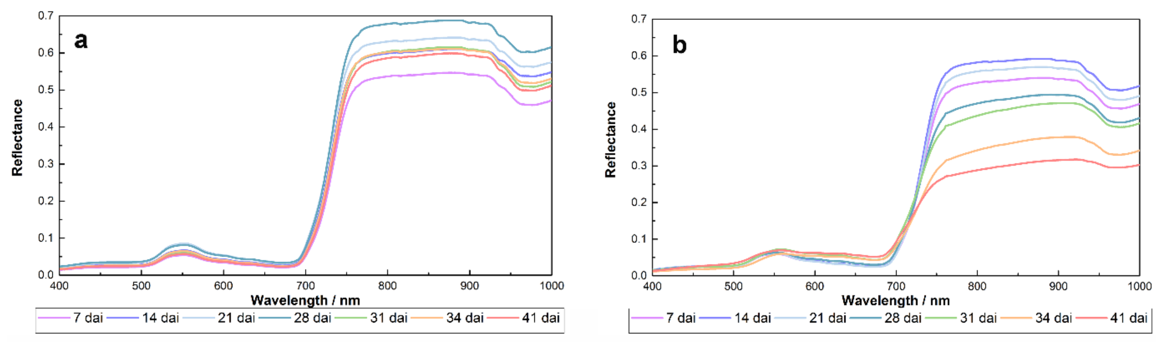
To our knowledge, this work may be the first attempt to track progressive host–pathogen interaction in the continuous hyperspectral observations. By using the wavelet-based feature extraction approach, a series of independent wavelet spectral features were extracted to characterize foliar biophysical dynamics caused by yellow rust infestation. In the process of CWT, the Mexican Hat mother wavelet fitted well with the absorption features of the original spectral responses of rust infestation, and the best capturing of changes on shape of spectral signals caused by the infestation development could be achieved by changing scale factors. In this study, CWT was implemented for 10 scales. The wavelet signatures at the scales of 2–5 retained a large amount of basic information of the original spectral reflectance and were useful at providing reliable responses pertaining to disease detection. These findings are also in agreement with the research by Zhang et al. [18].

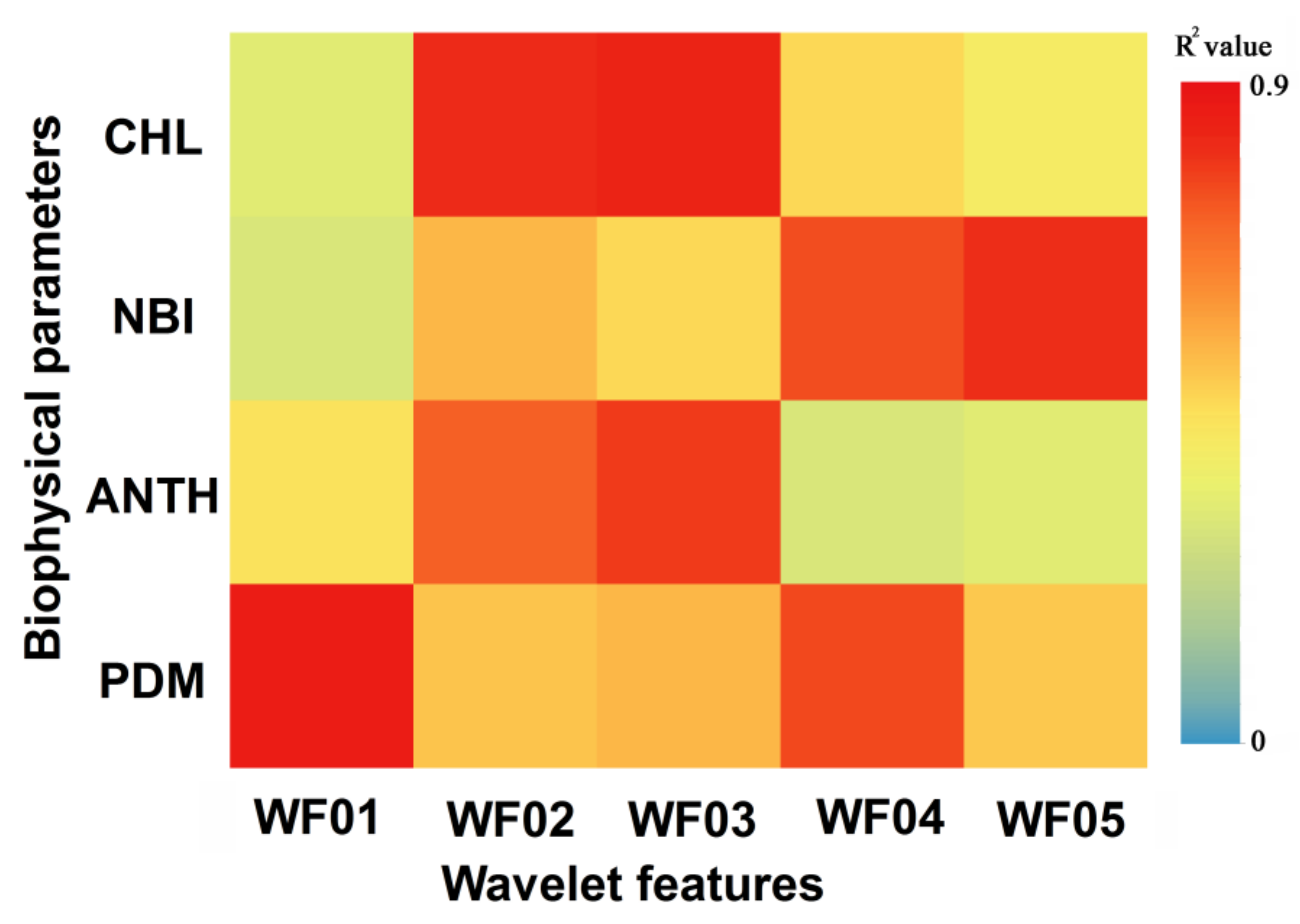
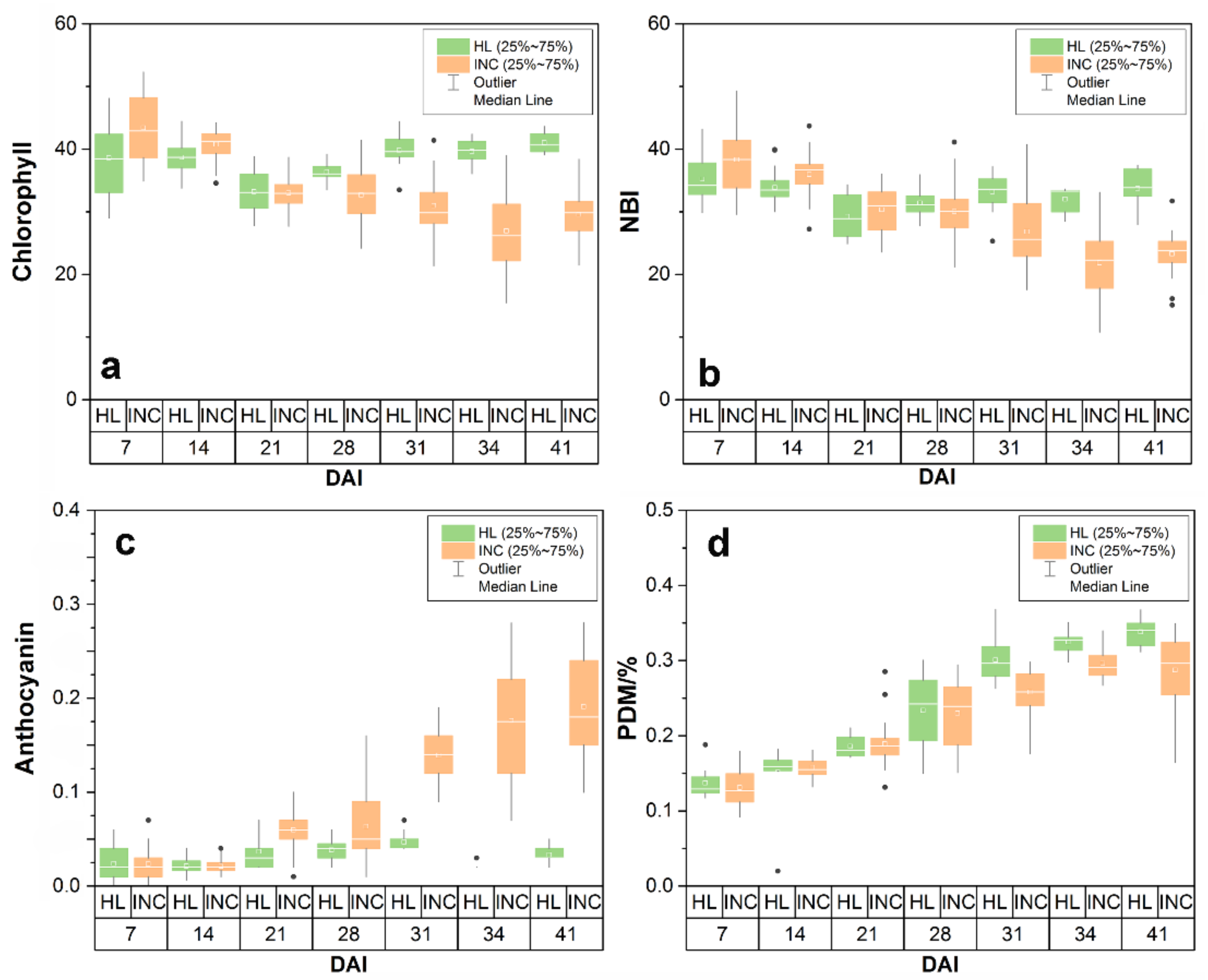
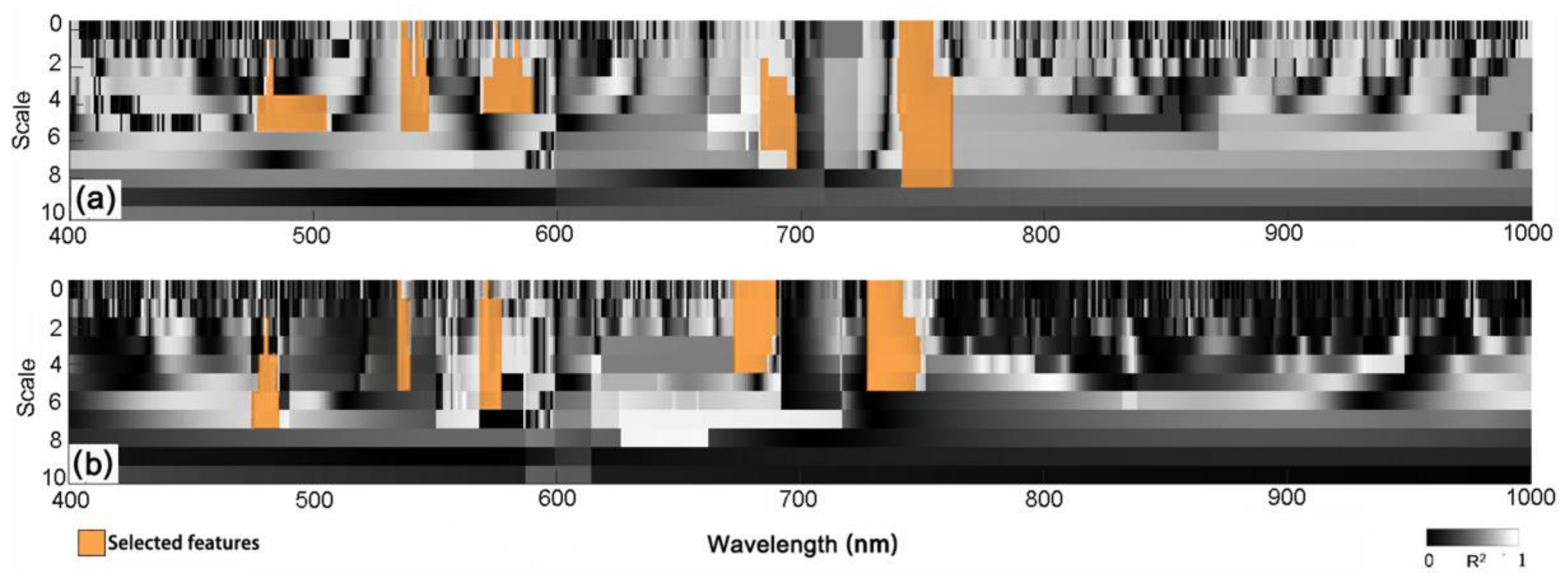
The identified WRSFs performed well in characterizing these progressive spectral responses of foliar biophysical changes caused by rust infestation (Figure 5). The ANOVA and univariate correlation analysis suggest that variations in foliar biophysical parameters induced by rust, such as chlorophyll content, anthocyanin content, nutrients, and dry matter accumulation, are best described by combining the extracted WRSFs from the hyperspectral perspective. Specifically, anthocyanin is the first detectable pigment induced by foliar stresses, and the increase of anthocyanin content can be detected by the WF03 between 573–584 nm. Additionally, the pathogens that attack various organs and tissues on leaves produce effects on plant structure and dry matter accumulation. The wavelet coefficients at the region of 478–496 nm, 683–697 nm, and 739–761 nm in the process of rust infestation prove that the impact of rust infestation on dry matter content and the upward movement of nitrogen could be detected by combining the WF01, WF04, and WF05. Meanwhile, pathogens do interfere with photosynthesis by affecting the chloroplasts and cause their degeneration, which are presented by the wavelet coefficient decrease of WF02 at 535–548 nm. This finding is also consistent with Sawut et al. [41]’s study, which reported the yellow bands near 550 nm are sensitive to photosynthetic pigments and have great potential in early plant stress detection.

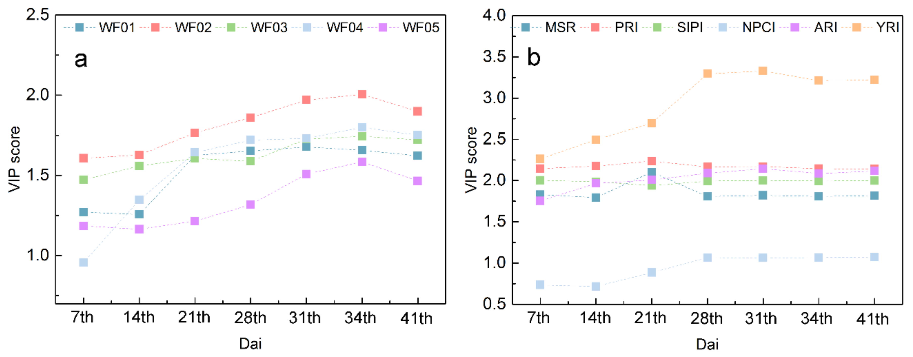
The PLSR models have been successfully used for DR estimations in the progression of yellow rust infestation. The results show that the WRSFs-PLSR model outperformed the VIs-PLSR on rust retrieving. More importantly, compared with VIs-PLSR, the WRSFs-PLSR provides apt pathological and biophysical information in the DR estimation procedure based on the VIP method. The analysis of importance in WRSFs measured by VIP scores has shown that the highest score structures for the early inoculation stage (before 14th dai) were contributed by WF02 and WF03 which are sensitive to CHL and ANTH. Additionally, as the symptoms became visible (after 21st dai), WF01 and WF04 which respond to PDM and NBI, showed higher importance in the model fitness. Finally, in the mid–late stage (28th–34th dai), because the rust spores rolled and ruptured the foliar epidermis, the importance of WF05, which is sensitive to the foliar structure rapidly increased. These importance dynamics in VIP scores during the PLSR analysis are consistent with the pathological progress of rust reported in related researches [7,12,51,52]. Furthermore, it was noteworthy that, in many cases, the shape-based wavelet features had been proven have greater robustness than VIs features. For example, Zhang, et al.’s study reported that, compared with traditional VIs or other spectral features, such as first-order derivative spectral and continuum removal features, no normalization procedure is needed for the application of the wavelet features, which makes them more robust in dealing with noises interferences [53]. This finding also partially supports our new proposed WRSFs that was more notable robust and sensitive to the foliar biophysical dynamics caused by the progressive infestation of yellow rust comparing with traditional VIs.

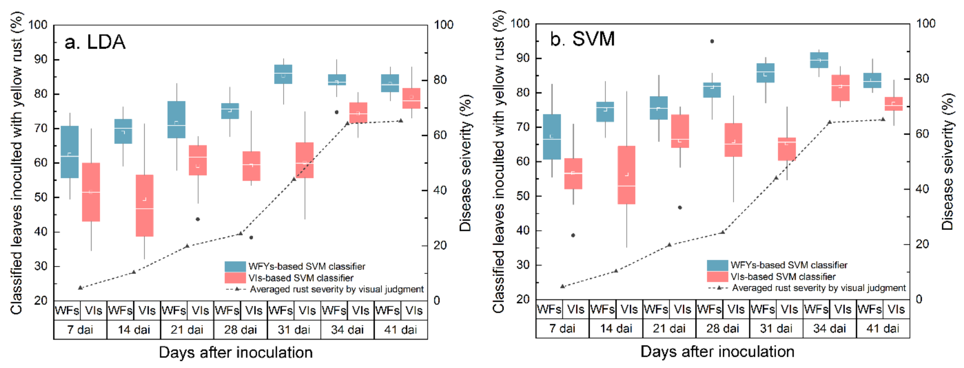
The efficiency of each kind of feature space in tracking rust lesions was evaluated using the identified WRSFs and VIs as input feature space in LDA and SVM classification methods. Compared to the LDA with empirical risk minimization, structural risk minimization-based SVMs proved to be the most instrumental strategy for automatic differentiation between healthy leaves and leaves infested with yellow rust, especially in the pre-symptomatic stages. In addition, compared with the LDA frame, the kernel-based SVM classifier performed better in limited the effect of high entropy on the sample set, especially before the visible symptoms occurred on the leaves, which achieved accuracies 3.5–6.4% higher than the LDA classification in yellow rust detection in different measurement dai (Figure 7). These conclusions are also in agreement with previous studies [42,47]. More importantly, compared with the VIs-based feature space, the greater orthogonality of the feature space produced by the WRSFs resulted in a more stable margin hyperplane for separation. This enhanced the information content and increased the generalization ability of SVM in tracking rust development at different stages. Unlike the VIs which use ratios of two or three bands of the visible- and near infrared region to normalize variations in the magnitude of reflectance, the shape-based wavelet spectral features produced by CWT with optimal combinations of positions and scales are able to capture the comprehensive biophysical variations and spectral responses caused by disease, such as the chlorophyll concentration variations and corresponding “blue shifting” phenomenon in spectral domain [20,54]. This characteristic explains why the WRSFs-based model outperform the VIs for rust detection and differentiation. Our findings also suggest that, by using the WRSFs-based SVM model, the earliest detection of yellow rust infestation can be achieved in 7th dai, with the acceptable accuracies of 67.4% and 86.5% for ASD and Headwall measurements.

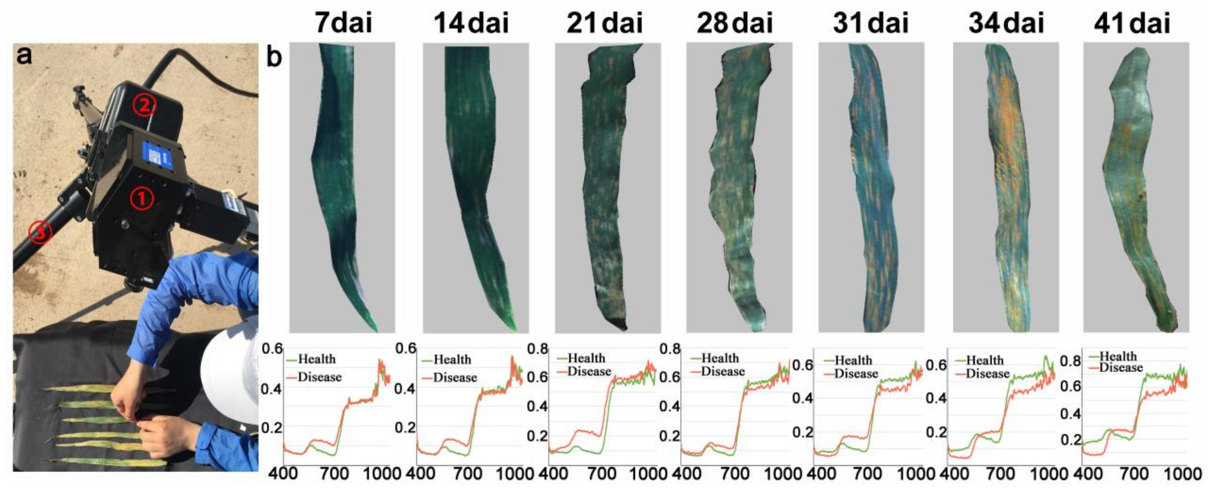
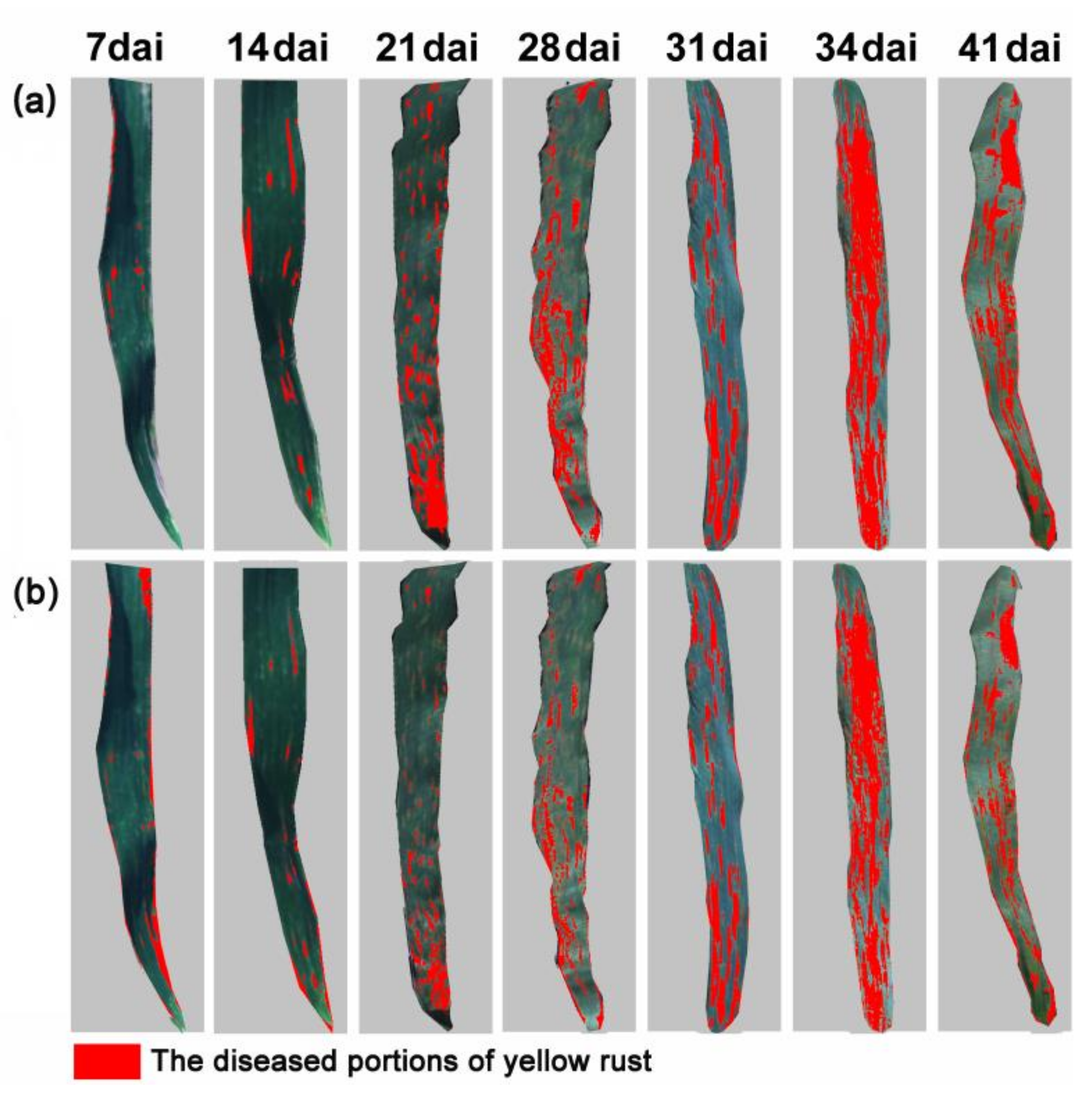
Comparing the spectral datasets of yellow rust collected in this study, there is much more noise in the detection of foliar symptoms in the non-imaging data obtained by the ASD spectroradiometer in comparison to the pixel-based spectral images collected by the Headwall spectrograph. The main explanation to this finding is that the spectral signatures measured by the spectroradiometer are the mean of the reflectance of both healthy and diseased plant tissues in single leaves. With imaging sensor systems, such as the Headwall spectrograph, a pixel-wise attribution of rust lesions and tissue is used. Therefore, the comparison of classification accuracy between the non-imaging and imaging datasets proven that the hyperspectral imaging system enabled detection of the small size of rust colonies, especially for the improvement of early disease monitoring. Meanwhile, because the proposed WRSFs include only the most relevant information of the infestation of yellow rust, the WRSFs-based models have better capacity of reducing the computational burden and achieving a near-real time diseases detection. These findings will lead to a better understanding of the pathogen–host interactions of yellow rust in field from the perspective of spectrum. However, although the inclusion of our findings can be carried out to indicate the pathologically related foliar lesion, the yellow rust-specific canopy structure characteristics were not explored in current study. Future work will evaluate the canopy structure effect on the contextual findings in order to conduct an operational application on UVA or space platform. Therefore, in this study, there were no additional nondestructive measurements in the field used for operational application.

5. Conclusions

This study proposed a new shape-based WRSFs from the wavelet transformed reflectance spectra of winter wheat leaves inoculated with yellow rust. The identified wavelet features in WRSFs are capable of capturing and tracking rust related biophysical indices (CHL, ANTH, NBI, and PDM) during development of the host–pathogen interaction. The performance of WRSFs as input feature space for disease severity estimation and lesions detection of rust was evaluated and compared with traditional VIs that sensitive to disease infestation. Our findings suggest that the WRSFs-PLSR model provide insight into specific host–pathogen interaction during rust development progress, which is more effective than VIs-PLSR model in DR estimation (R² > 0.78). For the rust lesion detection, the WRSFs-based feature space performed best for both LDA and SVM classification frame with overall accuracies of 81.8% and 86.6%, respectively. Unlike the traditional techniques, the CWT-based technique for WRSFs extraction is simple and straightforward to reflect spectral signals. As no predetermination of wavelength delimitation or other parameterization is required. The practical WRSFs have greater robustness for better understanding the pathological progress in tracking the rust development with hyperspectral data from various sensors. This method has the potential to be applicable to others plan–pathogen systems at the leaf scale. Nonetheless, its applicability from air- or space-borne remote sensing platforms requires proof and should be examined in future studies.

References

1. Gaspar, T.; Franck, T.; Bisbis, B.; Kevers, C.; Jouve, L.; Hausman, J.F.; Dommes, J. Concepts in plant stress physiology. Application to plant tissue cultures. Plant Growth Regul. 2002, 37, 263–285. [Google Scholar] [CrossRef]
2. Chaerle, L.; Van Der Straeten, D. Imaging techniques and the early detection of plant stress. Trends Plant Sci. 2000, 5, 495–501. [Google Scholar] [CrossRef]
3. Devadas, R.; Lamb, D.W.; Simpfendorfer, S.; Backhouse, D. Evaluating ten spectral vegetation indices for identifying rust infection in individual wheat leaves. Precis. Agric. 2009, 10, 459–470. [Google Scholar] [CrossRef]
4. Franke, J.; Menz, G. Multi-temporal wheat disease detection by multi-spectral remote sensing. Precis. Agric. 2007, 8, 161–172. [Google Scholar] [CrossRef]
5. Huang, W.; Davidw, L.; Zheng, N.; Zhang, Y.; Liu, L.; Wang, J. Identification of yellow rust in wheat using in-situ spectral reflectance measurements and airborne hyperspectral imaging. Precis. Agric. 2007, 8, 187–197. [Google Scholar] [CrossRef]
6. Cao, X.; Luo, Y.; Zhou, Y.; Duan, X.; Cheng, D. Detection of powdery mildew in two winter wheat cultivars using canopy hyperspectral reflectance. Crop Prot. 2013, 45, 124–131. [Google Scholar] [CrossRef]
7. Rampitsch, C.; Bykova, N.V.; McCallum, B.; Beimcik, E.; Ens, W. Analysis of the wheat and Puccinia triticina (leaf rust) proteomes during a susceptible host-pathogen interaction. Proteomics 2006, 6, 1897–1907. [Google Scholar] [CrossRef] [PubMed]
8. Grant, M.; Mansfield, J. Early events in host-pathogen interactions. Curr. Opin. Plant Biol. 1999, 2, 312–319. [Google Scholar] [CrossRef]
9. Mahlein, A.K.; Rumpf, T.; Welke, P.; Dehne, H.W.; Plümer, L.; Steiner, U.; Oerke, E.C. Development of spectral indices for detecting and identifying plant diseases. Remote Sens. Environ. 2013, 128, 21–30. [Google Scholar] [CrossRef]
10. Shi, Y.; Huang, W.; Luo, J.; Huang, L.; Zhou, X. Detection and discrimination of pests and diseases in winter wheat based on spectral indices and kernel discriminant analysis. Comput. Electron. Agric. 2017, 141, 171–180. [Google Scholar] [CrossRef]
11. Mcintosh, R.A.; Wellings, C.R. Wheat rust resistance—The continuing challenge. Aust. Plant Pathol. 1986, 15, 1–8. [Google Scholar] [CrossRef]
12. Staples, R.C.; Yaniv, Z.; Bushnell, W.R. Spore germination and ribosomal activity in the rust fungi I. Comparison of a bean rust fungus and a culturable wheat rust fungus. Physiol. Plant Pathol. 1972, 2, 27–35. [Google Scholar] [CrossRef]
13. Alvarez, A.M. Integrated approaches for detection of plant pathogenic bacteria and diagnosis of bacterial diseases. Annu. Rev. Phytopathol. 2004, 42, 339–366. [Google Scholar] [CrossRef] [PubMed]
14. Behmann, J.; Steinrücken, J.; Plümer, L. Detection of early plant stress responses in hyperspectral images. ISPRS J. Photogramm. Remote Sens. 2014, 93, 98–111. [Google Scholar] [CrossRef]
15. Bravo, C.; Moshou, D.; Oberti, R.; West, J.; Mccartney, A.; Bodria, L.; Ramon, H. Foliar disease detection in the field using optical sensor fusion. Eur. J. Endocrinol. 2004, 133, 467–474. [Google Scholar]
16. Elmasry, G.; Wang, N.; Vigneault, C.; Qiao, J.; Elsayed, A. Early detection of apple bruises on different background colors using hyperspectral imaging. LWT Food Sci. Technol. 2008, 41, 337–345. [Google Scholar] [CrossRef]
17. Kobayashi, T.; Kanda, E.; Kitada, K.; Ishiguro, K.; Torigoe, Y. Detection of rice panicle blast with multispectral radiometer and the potential of using airborne multispectral scanners. Phytopathology 2001, 91, 316–323. [Google Scholar] [CrossRef] [PubMed]
18. Zhang, J.; Yuan, L.; Pu, R.; Loraamm, R.W.; Yang, G.; Wang, J. Comparison between wavelet spectral features and conventional spectral features in detecting yellow rust for winter wheat. Comput. Electron. Agric. 2014, 100, 79–87. [Google Scholar] [CrossRef]
19. Cheng, T.; Rivard, B.; Sánchez-Azofeifa, G.A. Spectroscopic determination of leaf water content using continuous wavelet analysis. In Proceedings of the 2010 IEEE International Geoscience and Remote Sensing Symposium, Honolulu, HI, USA, 25–30 July 2010; pp. 659–670. [Google Scholar]
20. Shi, Y.; Huang, W.; Zhou, X. Evaluation of wavelet spectral features in pathological detection and discrimination of yellow rust and powdery mildew in winter wheat with hyperspectral reflectance data. J. Appl. Remote Sens. 2017, 11, 026025. [Google Scholar] [CrossRef]
21. Zhang, J.C.; Lin, Y.; Wang, J.H.; Huang, W.J.; Chen, L.P.; Zhang, D.Y. Spectroscopic leaf level detection of powdery mildew for winter wheat using continuous wavelet analysis. J. Integr. Agric. 2012, 11, 1474–1484. [Google Scholar] [CrossRef]
22. Liang, D.; Yang, Q.; Huang, W.; Peng, D.; Zhao, J.; Huang, L.; Zhang, D.; Song, X. Estimation of leaf area index based on wavelet transform and support vector machine regression in winter wheat. Infrared Laser Eng. 2015, 44, 335–340. [Google Scholar]
23. Pu, R.; Gong, P. Wavelet transform applied to EO-1 hyperspectral data for forest LAI and crown closure mapping. Remote Sens. Environ. 2004, 91, 212–224. [Google Scholar] [CrossRef]
24. Singh, S.K.; Hoyosvillegas, V.; Ray, J.D.; Smith, J.R.; Fritschi, F.B. Quantification of leaf pigments in soybean (Glycine max (L.) Merr.) based on wavelet decomposition of hyperspectral features. Field Crops Res. 2013, 149, 20–32. [Google Scholar] [CrossRef]
25. Zhang, D. Comparison of spectral indices and wavelet transform for estimating chlorophyll content of maize from hyperspectral reflectance. J. Appl. Remote Sens. 2013, 7, 073575. [Google Scholar]
26. Cerovic, Z.G.; Masdoumier, G.; Ghozlen, N.B.; Latouche, G. A new optical leaf-clip meter for simultaneous non-destructive assessment of leaf chlorophyll and epidermal flavonoids. Physiol. Plant. 2012, 146, 251–260. [Google Scholar] [CrossRef] [PubMed]
27. Bürling, K.; Cerovic, Z.G.; Cornic, G.; Ducruet, J.M.; Noga, G.; Hunsche, M. Fluorescence-based sensing of drought-induced stress in the vegetative phase of four contrasting wheat genotypes. Environ. Exp. Bot. 2013, 89, 51–59. [Google Scholar] [CrossRef]
28. Graeff, S.; Link, J.; Claupein, W. Identification of powdery mildew (Erysiphe graminis sp. tritici) and take-all disease (Gaeumannomyces graminis sp. tritici) in wheat (Triticum aestivum L.) by means of leaf reflectance measurements. Open Life Sci. 2006, 1, 275–288. [Google Scholar] [CrossRef]
29. Malthus, T.J.; Madeira, A.C. High resolution spectroradiometry: Spectral reflectance of field bean leaves infected by Botrytis fabae. Remote Sens. Environ. 1993, 45, 107–116. [Google Scholar] [CrossRef]
30. Yang, C.M.; Cheng, C.H.; Chen, R.K. Changes in spectral characteristics of rice canopy infested with brown planthopper and leaffolder. Crop Sci. 2007, 47, 329–335. [Google Scholar] [CrossRef]
31. Koger, C.H.; Bruce, L.M.; Shaw, D.R.; Reddy, K.N. Wavelet analysis of hyperspectral reflectance data for detecting pitted morningglory (Ipomoea lacunosa) in soybean (Glycine max). Remote Sens. Environ. 2003, 86, 108–119. [Google Scholar] [CrossRef]
32. Chen, B.; Wang, K.; Li, S.; Wang, J.; Bai, J.; Xiao, C.; Lai, J. Spectrum characteristics of cotton canopy infected with verticillium wilt and inversion of severity level. In Proceedings of the IFIP TC 12 International Conference on Computer and Computing Technologies in Agriculture (CCTA 2007), Wuyishan, China, 18–20 August 2007; pp. 1169–1180. [Google Scholar]
33. Gamon, J.A.; Peñuelas, J.; Field, C.B. A narrow-waveband spectral index that tracks diurnal changes in photosynthetic efficiency. Remote Sens. Environ. 1992, 41, 35–44. [Google Scholar] [CrossRef]
34. Penuelas, J.; Baret, F.; Filella, I. Semiempirical indexes to assess carotenoids chlorophyll-a ratio from leaf spectral reflectance. Photosynthetica 1995, 31, 221–230. [Google Scholar]
35. Lewis, H.G.; Brown, M. A generalized confusion matrix for assessing area estimates from remotely sensed data. Int. J. Remote Sens. 2001, 22, 3223–3235. [Google Scholar] [CrossRef]
36. Merton, R.; Huntington, J.; Merton, R. Early simulation results of the ARIES-1 satellite sensor for multi-temporal vegetation research derived from AVIRIS. In Proceedings of the Eighth Annual JPL Airborne Earth Science Workshop, Pasadena, CA, USA, 9–11 February 1999; pp. 8–14. [Google Scholar]
37. Daughtry, C.S.T.; Walthall, C.L.; Kim, M.S.; Colstoun, E.B.D.; Mcmurtrey, J.E. Iii, Estimating corn leaf chlorophyll concentration from leaf and canopy reflectance. Remote Sens. Environ. 2000, 74, 229–239. [Google Scholar] [CrossRef]
38. Huang, W.; Guan, Q.; Luo, J.; Zhang, J. New optimized spectral indices for identifying and monitoring winter wheat diseases. IEEE J. Sel. Top. Appl. Earth Obs. Remote Sens. 2014, 7, 2516–2524. [Google Scholar] [CrossRef]
39. Sawut, M.; Ghulam, A.; Tiyip, T.; Zhang, Y.J.; Ding, J.L.; Zhang, F.; Maimaitiyiming, M. Estimating soil sand content using thermal infrared spectra in arid lands. Int. J. Appl. Earth Obs. Geoinform. 2014, 33, 203–210. [Google Scholar] [CrossRef]
40. Peerbhay, K.Y.; Mutanga, O.; Ismail, R. Commercial tree species discrimination using airborne AISA Eagle hyperspectral imagery and partial least squares discriminant analysis (PLS-DA) in KwaZulu–Natal, South Africa. ISPRS J. Photogramm. Remote Sens. 2013, 79, 19–28. [Google Scholar] [CrossRef]
41. Maimaitiyiming, M.; Ghulam, A.; Bozzolo, A.; Wilkins, J.L.; Kwasniewski, M.T.; Maimaitiyiming, M.; Ghulam, A.; Bozzolo, A.; Wilkins, J.L.; Kwasniewski, M.T. Early detection of plant physiological responses to different levels of water stress using reflectance spectroscopy. Remote Sens. 2017, 9, 745. [Google Scholar] [CrossRef]
42. Laurin, G.V.; Chen, Q.; Lindsell, J.A.; Coomes, D.A.; Frate, F.D.; Guerriero, L.; Pirotti, F.; Valentini, R. Above ground biomass estimation in an African tropical forest with Lidar and hyperspectral data. ISPRS J. Photogramm. Remote Sens. 2014, 89, 49–58. [Google Scholar] [CrossRef]
43. Wold, S.; Sjöström, M.; Eriksson, L. PLS-regression: A basic tool of chemometrics. Chemom. Intell. Lab. Syst. 2001, 58, 109–130. [Google Scholar] [CrossRef]
44. Yao, Q.; Guan, Z.; Zhou, Y.; Tang, J.; Hu, Y.; Yang, B. Application of support vector machine for detecting rice diseases using shape and color texture features. In Proceedings of the 2009 International Conference on Engineering Computation, Bangi, Malaysia, 5–7 August 2009; pp. 79–83. [Google Scholar]
45. Liu, Z.Y.; Wu, H.F.; Huang, J.F. Application of neural networks to discriminate fungal infection levels in rice panicles using hyperspectral reflectance and principal components analysis. Comput. Electron. Agric. 2010, 72, 99–106. [Google Scholar] [CrossRef]
46. Seelan, S.K.; Laguette, S.; Casady, G.M.; Seielstad, G.A. Remote sensing applications for precision agriculture: A learning community approach. Remote Sens. Environ. 2003, 88, 157–169. [Google Scholar] [CrossRef]
47. Bandos, T.V.; Bruzzone, L.; Camps-Valls, G. Classification of hyperspectral images with regularized linear discriminant analysis. IEEE Trans. Geosci. Remote Sens. 2009, 47, 862–873. [Google Scholar] [CrossRef]
48. Tong, S. Support vector machine active learning for image retrieval. In Proceedings of the ACM International Conference on Multimedia, Ottawa, ON, Canada, 30 September–5 October 2001; pp. 107–118. [Google Scholar]
49. Amari, S.; Wu, S. Improving support vector machine classifiers by modifying kernel functions. Neural Netw. 1999, 12, 783–789. [Google Scholar] [CrossRef]
50. Rumpf, T.; Mahlein, A.K.; Steiner, U.; Oerke, E.C.; Dehne, H.W.; Plümer, L. Early detection and classification of plant diseases with Support Vector Machines based on hyperspectral reflectance. Comput. Electron. Agric. 2010, 74, 91–99. [Google Scholar] [CrossRef]
51. Huang, W.; Huang, M.; Liu, L.; Wang, J.; Zhao, C.; Wang, J. Inversion of the severity of winter wheat yellow rust using proper hyper spectral index. Trans. Chin. Soc. Agric. Eng. 2005, 21, 97–103. [Google Scholar]
52. Zhang, J.; Pu, R.; Huang, W.; Yuan, L.; Luo, J.; Wang, J. Using in-situ hyperspectral data for detecting and discriminating yellow rust disease from nutrient stresses. Field Crops Res. 2012, 134, 165–174. [Google Scholar] [CrossRef]
53. Zhang, J.; Huang, Y.; Li, Z.; Liu, P.; Yuan, L. Noise-resistant spectral features for retrieving foliar chemical parameters. IEEE J. Sel. Top. Appl. Earth Obs. Remote Sens. 2017, 10, 5369–5380. [Google Scholar] [CrossRef]
54. Blackburn, G.A.; Ferwerda, J.G. Retrieval of chlorophyll concentration from leaf reflectance spectra using wavelet analysis. Remote Sens. Environ. 2008, 112, 1614–1632. [Google Scholar] [CrossRef]
Figure 1. (a) The setup of the Headwall system: ①. Headwall visible to near infrared (VNIR) imagining sensor; ②. Pan & Tilt; ③. The tripod. (b) The true color composite image of the leave composited by raw hyperspectral images. The second row shows the comparison of spectral reflectance between the healthy area and diseased area of the leaves.
Remotesensing 10 00525 g001
Figure 2. Averaged leaf spectra for (a) healthy- and (b) rust infected-leaves at different days after infestation (dai).
Remotesensing 10 00525 g002
Figure 3. Comparisons of (a) chlorophyll index; (b) nitrogen balance index (NBI); (c) anthocyanin index; (d) percentile dry matter (PDM) between healthy leaves and leaves inoculated with yellow rust. The default units for chlorophyll, nitrogen balance index and anthocyanin are from the Duelax instrument.
Remotesensing 10 00525 g003
Figure 4. Correlation scalogram of continuous wavelet analysis for WRSFs extraction from (a) ASD and (b) Headwall dataset. This scalogram indicates the determination coefficients (R2) between wavelet power and disease ration (DR). The highest 5% were highlighted in orange identifying wavelet feature regions.
Remotesensing 10 00525 g004
Figure 5. Correlation analysis (in coefficient of determination R2) of individual wavelet features with foliar components parameters (NBI, CHL, ANTH, PDM).
Remotesensing 10 00525 g005
Figure 6. Variable importance in projection (VIP) scores of (a) wavelet-based rust spectral feature sets (WRSFs) and (b) vegetation indices (VIs) spectral features explaining yellow rust disease ratio (DR) in separate partial least square regression (PLSR) models for each date after inoculation sampled (dai).
Remotesensing 10 00525 g006
Figure 7. Effect of time since inoculation on the classification accuracy results of ASD spectroradiometer-derived (a) linear discriminant analysis (LDA) and (b) support vector machine (SVM) model for the identification of diseased leaves inoculated with yellow rust versus healthy leaves. The box-plot of the classification accuracies are produced by the cross-validation. The dash line represents the averaged rust severity (DR) measured per sampling date.
Remotesensing 10 00525 g007
Figure 8. Extraction of rust diseased area produced by (a) WRSFs-based SVM and (b) VIs-based SVM from hyperspectral images of leaves at different dai.
Remotesensing 10 00525 g008